Decadal Changes of Wind Stress over the Southern Ocean Associated with AntarcticOzone Depletion

XIAO-YI YANG

Key Laboratory of Tropical Marine Environmental Dynamics, South China Sea Institute of Oceanology, Chinese Academy ofSciences, Guangzhou, China

RUI XIN HUANG

Department of Physical Oceanography, Woods Hole Oceanographic Institution, Woods Hole, Massachusetts

DONG XIAO WANG

Key Laboratory of Tropical Marine Environmental Dynamics, South China Sea Institute of Oceanology, Chinese Academy ofSciences, Guangzhou, China

(Manuscript received 19 April 2006, in final form 15 September 2006)

ABSTRACT

Using 40-yr ECMWF Re-Analysis (ERA-40) data and in situ observations, the positive trend of SouthernOcean surface wind stress during two recent decades is detected, and its close linkage with spring Antarcticozone depletion is established. The spring Antarctic ozone depletion affects the Southern Hemispherelower-stratospheric circulation in late spring/early summer. The positive feedback involves the strengthen-ing and cooling of the polar vortex, the enhancement of meridional temperature gradients and the meridi-onal and vertical potential vorticity gradients, the acceleration of the circumpolar westerlies, and thereduction of the upward wave flux. This feedback loop, together with the ozone-related photochemicalinteraction, leads to the upward tendency of lower-stratospheric zonal wind in austral summer. In addition,the stratosphere–troposphere coupling, facilitated by ozone-related dynamics and the Southern AnnularMode, cooperates to relay the zonal wind anomalies to the upper troposphere. The wave–mean flowinteraction and the meridional circulation work together in the form of the Southern Annular Mode, whichtransfers anomalous wind signals downward to the surface, triggering a striking strengthening of surfacewind stress over the Southern Ocean.

1. Introduction

More and more evidence shows that anthropogenicinfluence is an important cause of recent climatechanges. The discovery of dramatic seasonal ozone lossin the Antarctic is a good example. According to theheterogeneous chemistry theory proposed by Crutzenand Arnold (1986), McElroy et al. (1986), and Solomonet al. (1986), chlorine- and bromine-catalyzed photo-chemical reactions destroy most of the stratosphericozone in the Antarctic region. The increasing content

of atmospheric chlorine produced by human activities,therefore, has been identified as a crucial player for thespringtime ozone hole that developed in the late 1970s(Solomon 1999; Albritton et al. 1998).

Many studies have discussed the impacts of severeAntarctic ozone depletion on global climate change.Randel and Wu (1999) documented a steplike coolingduring Antarctic spring in the lower stratosphere,which can be explained through model simulations asa radiative response to the observed ozone loss(Shine 1986; Mahlmann et al. 1994; Langematz 2000).Ramaswamy et al. (2001) concluded that more thanthree-quarters of the trend in lower-stratospheric tem-perature over the period 1979–90 may be attributed toozone depletion. Observations indicate that the Ant-arctic vortex has strengthened over recent decades(Waugh et al. 1999; Zhou et al. 2000). Thompson and

Corresponding author address: Xiao-Yi Yang, Key Laboratoryof Tropical Marine Environmental Dynamics, South China SeaInstitute of Oceanology, Chinese Academy of Sciences, 164 WestXingang Road, Guangzhou 510301, China.E-mail: yxy@scsio.ac.cn

15 JULY 2007 Y A N G E T A L . 3395

DOI: 10.1175/JCLI4195.1

© 2007 American Meteorological Society

JCLI4195

Solomon (2002, hereafter TS02) argued that photo-chemical ozone loss may be the main external forcingresponsible for driving this trend, the high polarity ofthe Southern Annular Mode (SAM), and the most sig-nificant tropospheric trends. Through numerical simu-lations, Gillett and Thompson (2003, hereafter GT03)further discussed the impacts of Antarctic ozone lossupon climate at the earth’s surface and in the strato-sphere.

At present, however, the dynamics of Antarcticozone depletion and its climatic implication are farfrom being resolved, partly due to the complicated in-terplay between Antarctic ozone and other climatevariables, as well as the indistinct stratosphere–tropo-sphere coupling processes.

This study is mainly motivated by Huang et al.(2006), who found that the wind energy input to theAntarctic Circumpolar Current (ACC) increased re-markably during recent decades. Since wind energy in-put to the ocean is the primary source of external me-chanical energy driving the oceanic general circulation(Huang 1998, 2004; Wunsch and Ferrari 2004), this in-spires us to explore the causes of the decadal change ofthe surface wind stress over the Southern Ocean.

In our discussion of Southern Hemisphere (SH) cli-mate phenomena, we define austral spring as Septem-ber–November, austral summer as December–Febru-ary, and so on. We define an “austral year” as begin-ning on 1 July.

In this work, we present evidence to demonstrate thefollowing:

1) The positive trends of surface wind stress over theSouthern Ocean (45°�60°S) exhibit strong season-ality with the peak in austral summer (January).

2) This trend is closely related to the spring Antarcticozone depletion.

3) There exists an ozone-related thermodynamic anddynamical feedback mechanism in the lower strato-spheric Antarctic. The resulting anomalous windcan propagate downward to the surface through theSAM-related wave–mean flow interaction and me-ridional circulation.

The outline of the work is as follows: The data andmethods applied are introduced in section 2. In section3a, the time series and trends of Antarctic ozone andwind stress over the Southern Ocean are presented,including the variability in their seasonal cycles. Thenwe describe the lower-stratospheric circulation varia-tion associated with Antarctic ozone depletion in sec-tion 3b. Next, the downward propagation of zonal-windanomalies is described in section 3c. Finally, section 4presents the conclusions and discussion.

2. Data and analysis technique

Some studies have indicated a deficiency of NationalCenters for Envrionmental Prediction–National Centerfor Atmospheric Research (NCEP–NCAR) reanalysisdata in representing the long-term climate change athigh and midlatitudes of the Southern Hemisphere(Hines et al. 2000; Marshall 2002, 2003). The problemarose from the assimilation of the Australian SurfacePressure Bogus Data (PAOBS) for the SH in which theobservations were erroneously shifted by 180° in longi-tude, affecting the period 1979–92. Marshall (2003) sug-gested that compared with NCEP–NCAR reanalysisdata, the 40-yr European Centre for Medium-RangeWeather Forecasts (ECMWF) Re-Analysis (ERA-40)dataset provides an improved representation of SHhigh-latitude atmospheric circulation variability. As aresult of satellite data assimilation after 1978 and ahigher level of skill, ERA-40 is superior to the NCEP–NCAR dataset for the research of long-term climatechange in the SH extratropics. Therefore, the ERA-40monthly dataset is chosen in this study.

Two monthly SAM indices are used in this study: thefirst one is a station-based index following the method-ology of Marshall (2003); the second one is derived byapplying EOF analysis to the 18-level SH extratropicalgeopotential height field [weighted by the square rootof the cosine of latitude, following Chung and Nigam(1999)] and taking respective time series of leadingmodes as the SAM indices [similar to the method ofThompson et al. (2005)].

To test the reliability of the trend analyses based onthe ERA-40 data, we also use other in situ observationsand satellite measurements, including the monthly sur-face wind speed at Macquarie Island (54.5°S, 158.9°E)from the Australian Government Bureau of Meteorol-ogy, Special Sensor Microwave Imager (SSM/I) satel-lite wind speed data, Total Ozone Mapping Spectrom-eter (TOMS) monthly total column ozone data, andSouth Pole CO2 data.

The linear trend is estimated as the linear regressioncoefficient of each grid point data on time. The signifi-cance level of trend is tested by applying the t-testmethod of Santer et al. (2000). Given the highly zonalsymmetry of the SH atmospheric circulation, the trendestimation and other analyses in this study are all basedon zonal-mean data.

The wind stress field is calculated from the 10-m Uwind and V wind, using the bulk formula, � ��0CD|V |V, where � and V denote the wind stress vectorand 10-m wind vector, respectively; |V| the wind speedat 10 m; and �0 the air density. The drag coefficient CD

3396 J O U R N A L O F C L I M A T E VOLUME 20

is calculated from the empirical formula (Garratt 1977),CD � 7.5 � 10�4 � 6.7 � 10�5 � |V | .

The Eliassen–Palm (EP) flux is computed from dailywind and temperature fields, using the following for-mula in spherical coordinates:

F� � �2�R2 cos2���

gU*V*;

Fp � �2�R3 cos2���

gf V*�*���S��p��1;

where R is the earth’s radius, g is the gravity, f theCoriolis parameter, � is latitude, � denotes potentialtemperature, and �s the global mean potential tempera-ture on a pressure surface. Note that to facilitatestraightforward physical interpretation we have addeda minus sign for the vertical component of the EP fluxfor the Southern Hemisphere so that the positive valueof vertical EP flux represents the upward wave forcingand poleward eddy heat flux. For the similar purpose,the Ertel’s potential vorticity (PV) in the SH is definedas (without the minus sign in the front)

P � g� f � ������

�p�.

3. Results

a. Wind stress trend and its seasonality

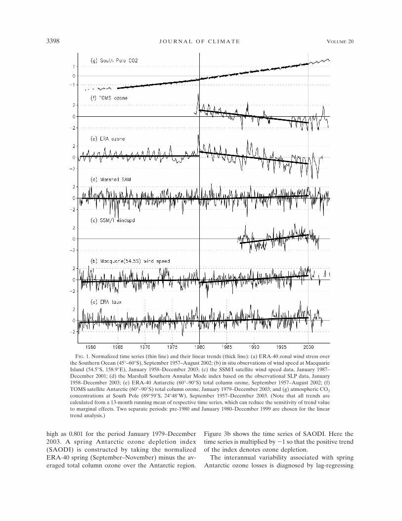
Figure 1 shows the various normalized time seriesand their linear trends. The trends are calculated fortwo distinct periods: prior to 1980 and 1980–99. Forclarity, trend coefficients are presented in Table 1, withthe bold phase and asterisk denoting the trends abovethe 95% significance level t test. It is clear that for thezonal wind stress (Taux) over the Southern Ocean(45°–60°S; Fig. 1a), the positive trend is statistically sig-nificant for the period 1980–99 only (Table 1). Al-though the ERA-40 dataset is preferred to the NCEP–NCAR dataset for long-term climate study, cautionsmust be taken in that ERA-40 data is also dominatedby model simulations in SH prior to 1979 (Bengtsson etal. 2004). As the satellite measurements have been as-similated since the late 1970s, the statistical results ofclimate change may be simply due to the data discrep-ancy in assimilation process for the pre- and post-1980periods. Therefore, the comparison of ERA-40 dataand in situ observation time series is needed to verifythe trend analysis. Both in situ observations (Fig. 1b)and satellite measurements (Fig. 1c) have significantupward trends after the 1980s, and the Macquarie windspeed trends are almost twice as much as those of theERA-40 zonal wind stress for the whole 40 years (see

Table 1). In addition, linear correlation analysis indi-cates the consistency of Macquarie observations andERA-40 wind stress, the correlation coefficients beingas high as 0.466 for the period from January 1958 toDecember 2001 (528 months). This confirms the ro-bustness of ERA-40 trends analysis. The MarshallSAM index (Fig. 1d) and the Antarctic (60°S polewardaveraged) total column ozone data (Fig. 1e for ERA-40and Fig. 1f for TOMS satellite data) also exhibit signifi-cant trends after the 1980s, though the ozone trend ismuch more pronounced than that of the SAM.

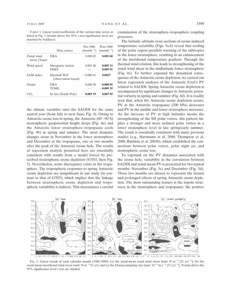
The seasonality of surface wind stress during 1980–2000 is delineated by calculating respective zonal-meanzonal (Fig. 2a) and meridional (Fig. 2b) wind stresstrends and Ekman pumping trends (Fig. 2c) for eachcalendar month. We see that all three variables exhibitstrong seasonality in their trends at midlatitudes, withthe strongest trends occurring in January. Secondarypeaks with marginally significant trends appear in May.More specifically, the zonal and meridional wind stresstrends in January are characterized by dipolelike pat-terns with the nodal latitude of �47.5°S, which, by re-ferring to the climatology (figures omitted), implies astrengthening of westerly and southerly wind stressespoleward of 47.5°S and slight weakening equatorwardof 47.5°S. As for the region of our interest—the South-ern Ocean (45°–60°S)—we see an overall upward trendof both wind stresses and Ekman pumping rate, and apoleward drift of the centers of maximum wind stress.

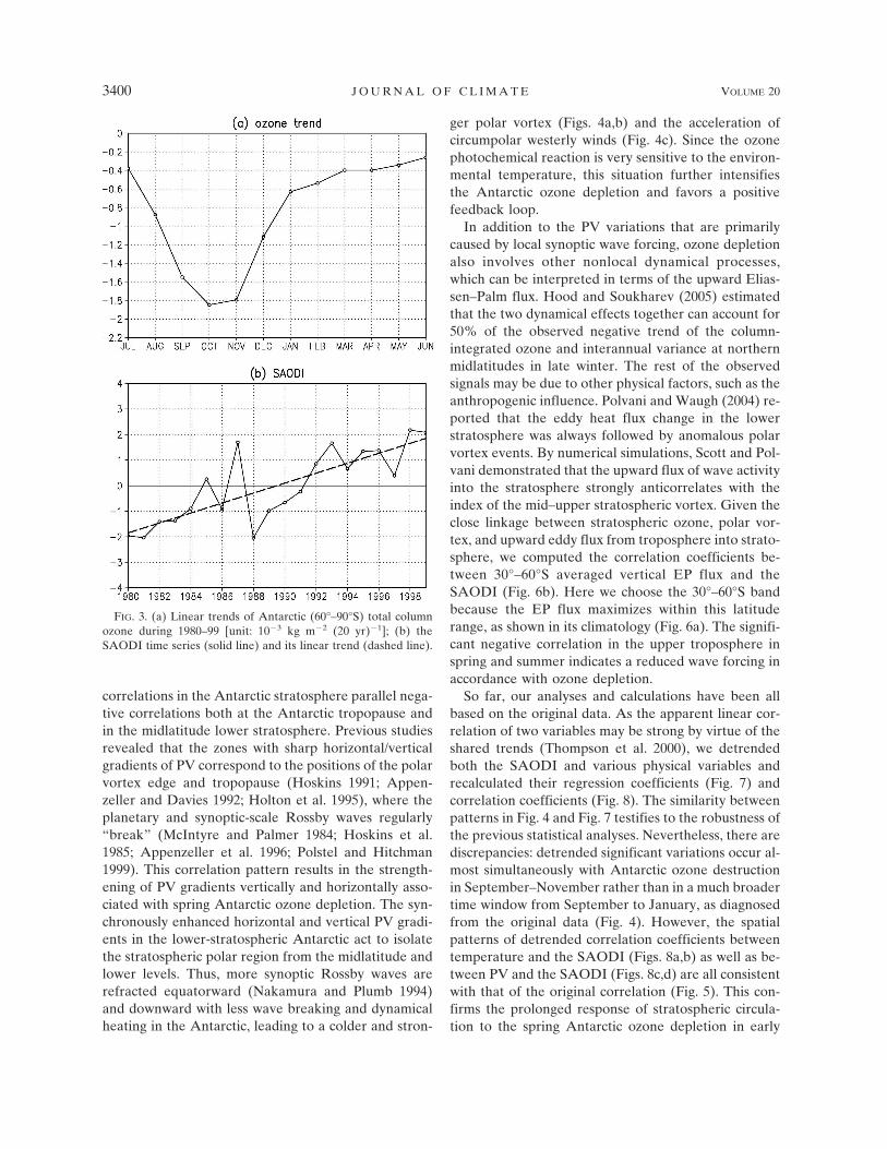
Previous studies showed that the Antarctic ozonedepletion culminates during spring [e.g., in situ obser-vations by Farman et al. (1985) and satellite measure-ments by Stolarski et al. (1986)]. The linear trend analy-sis of ERA-40 Antarctic (60°–90°S) total column ozonealso shows a strong seasonality (Fig. 3a) with the peakcentered in austral spring (September–November). Theseasonality in linear trend analyses suggests a possiblelinkage between the strengthening of wind stress overthe Southern Ocean in summer and the spring Antarc-tic ozone depletion. However, ozone depletion mainlyoccurs in the lower stratosphere. How could ozonedepletion in the lower stratosphere drive the surfacewind stress change with a lag of 1�2 months? Thisquestion deserves further investigation.

b. The interannual variability and long-term trendof the lower-stratospheric circulation associatedwith spring Antarctic ozone depletion

Since the ERA-40 ozone data assimilates both theTOMS total ozone and solar backscatter ultraviolet(SBUV), ozone profile (Kallberg et al. 2004), themonthly correlation between TOMS Antarctic ozone(Fig. 1f) and ERA-40 Antarctic ozone (Fig. 1e) is as

15 JULY 2007 Y A N G E T A L . 3397

high as 0.801 for the period January 1979–December2003. A spring Antarctic ozone depletion index(SAODI) is constructed by taking the normalizedERA-40 spring (September–November) minus the av-eraged total column ozone over the Antarctic region.

Figure 3b shows the time series of SAODI. Here thetime series is multiplied by �1 so that the positive trendof the index denotes ozone depletion.

The interannual variability associated with springAntarctic ozone losses is diagnosed by lag-regressing

FIG. 1. Normalized time series (thin line) and their linear trends (thick line): (a) ERA-40 zonal wind stress overthe Southern Ocean (45°–60°S), September 1957–August 2002; (b) in situ observations of wind speed at MacquarieIsland (54.5°S, 158.9°E), January 1958–December 2003; (c) the SSM/I satellite wind speed data, January 1987–December 2001; (d) the Marshall Southern Annular Mode index based on the observational SLP data, January1958–December 2003; (e) ERA-40 Antarctic (60°–90°S) total column ozone, September 1957–August 2002; (f)TOMS satellite Antarctic (60°–90°S) total column ozone, January 1979–December 2003; and (g) atmospheric CO2

concentrations at South Pole (89°59 S, 24°48 W), September 1957–December 2003. (Note that all trends arecalculated from a 13-month running mean of respective time series, which can reduce the sensitivity of trend valueto marginal effects. Two separate periods: pre-1980 and January 1980–December 1999 are chosen for the lineartrend analysis.)

3398 J O U R N A L O F C L I M A T E VOLUME 20

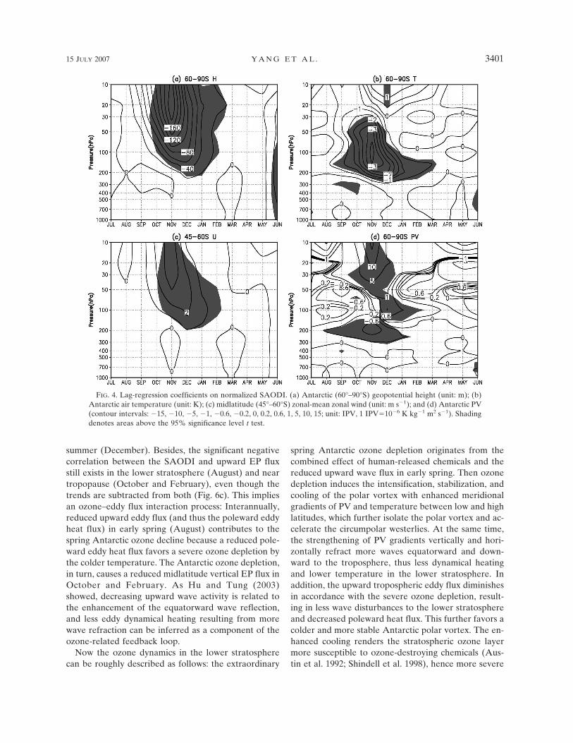
the climate variables onto the SAODI for the sameaustral year (from July to next June; Fig. 4). Owing toAntarctic ozone loss in spring, the Antarctic (60°–90°S)stratospheric geopotential height drops (Fig. 4a) andthe Antarctic lower stratosphere–tropopause cools(Fig. 4b) in spring and summer. The most dramaticchanges occur in November in the lower stratosphereand December at the tropopause, one or two monthsafter the peak of the Antarctic ozone hole. The resultsof regression analysis presented here are essentiallyconsistent with results from a model forced by pre-scribed stratospheric ozone depletion (GT03, their Fig.2). Nevertheless, some discrepancy exists in the tropo-sphere. The tropospheric responses to spring Antarcticozone depletion are insignificant in our study (in con-trast to that of GT03), which implies that the linkagebetween stratospheric ozone depletion and tropo-spheric variability is indirect. This necessitates a careful

examination of the stratosphere–troposphere couplingprocesses.

The latitude–altitude cross sections of ozone-inducedtemperature variability (Figs. 5a,b) reveal that coolingof the polar region parallels warming of the subtropicsin the lower stratosphere, resulting in an enhancementof the meridional temperature gradient. Through thethermal wind relation, this leads to strengthening of thezonal wind shear in the midlatitude lower stratosphere(Fig. 4c). To further expound the dynamical conse-quence of the Antarctic ozone depletion, we carried outlinear regression analyses of the Antarctic Ertel’s PVrelated to SAODI. Spring Antarctic ozone depletion isaccompanied by significant changes in Antarctic poten-tial vorticity in spring and summer (Fig. 4d). It is readilyseen that, when the Antarctic ozone depletion occurs,PV at the Antarctic tropopause (200 hPa) decreasesand PV in the middle and lower stratosphere increases.As the increase of PV at high latitudes means thestrengthening of the SH polar vortex, this pattern im-plies a stronger and more isolated polar vortex in alower stratosphere level in late spring/early summer.The result is essentially consistent with many previousstudies (e.g., Hartmann et al. 2000; Thompson et al.2000; Baldwin et al. 2003b), which established the con-nections between polar vortex, polar night jet, andstratospheric ozone loss.

To expound on the PV dynamics associated withthe ozone hole, variability in the correlation betweenSAODI and zonal-mean PV is presented for two typicalmonths: November (Fig. 5c) and December (Fig. 5d).These two months are chosen to represent the instantand prolonged effects of spring Antarctic ozone deple-tion. The most outstanding feature is the tripole struc-tures in the stratosphere and tropopause: the positive

FIG. 2. Linear trends of each calendar month (1980–2000): (a) the zonal-mean zonal wind stress [unit: N m�2 (21 yr)�1]; (b) thezonal-mean meridional wind stress (unit: N m�2/21 yr); and (c) the Ekman pumping rate [unit: 10�6 m s�1 (21 yr)�1]. Trends above the95% significance level t test are shaded.

TABLE 1. Linear trend coefficients of the various time series aslisted in Fig. 1 (trends above the 95% t-test significance level aredenoted by boldface).

Data sourcePre-1980

(month�1)Post-1980(month�1)

Zonal windstress (Taux)

ERA 0.000 82 0.002 68

Wind speed Macquarie station 0.001 40 0.005 11SSM/I — 0.009 91

SAM index Marshall SLP(observation based)

�0.000 41 0.0027

Ozone ERA 0.000 28 �0.008 81TOMS — �0.009 35

CO2 In situ (South Pole) 0.005 19 0.007 05

15 JULY 2007 Y A N G E T A L . 3399

correlations in the Antarctic stratosphere parallel nega-tive correlations both at the Antarctic tropopause andin the midlatitude lower stratosphere. Previous studiesrevealed that the zones with sharp horizontal/verticalgradients of PV correspond to the positions of the polarvortex edge and tropopause (Hoskins 1991; Appen-zeller and Davies 1992; Holton et al. 1995), where theplanetary and synoptic-scale Rossby waves regularly“break” (McIntyre and Palmer 1984; Hoskins et al.1985; Appenzeller et al. 1996; Polstel and Hitchman1999). This correlation pattern results in the strength-ening of PV gradients vertically and horizontally asso-ciated with spring Antarctic ozone depletion. The syn-chronously enhanced horizontal and vertical PV gradi-ents in the lower-stratospheric Antarctic act to isolatethe stratospheric polar region from the midlatitude andlower levels. Thus, more synoptic Rossby waves arerefracted equatorward (Nakamura and Plumb 1994)and downward with less wave breaking and dynamicalheating in the Antarctic, leading to a colder and stron-

ger polar vortex (Figs. 4a,b) and the acceleration ofcircumpolar westerly winds (Fig. 4c). Since the ozonephotochemical reaction is very sensitive to the environ-mental temperature, this situation further intensifiesthe Antarctic ozone depletion and favors a positivefeedback loop.

In addition to the PV variations that are primarilycaused by local synoptic wave forcing, ozone depletionalso involves other nonlocal dynamical processes,which can be interpreted in terms of the upward Elias-sen–Palm flux. Hood and Soukharev (2005) estimatedthat the two dynamical effects together can account for50% of the observed negative trend of the column-integrated ozone and interannual variance at northernmidlatitudes in late winter. The rest of the observedsignals may be due to other physical factors, such as theanthropogenic influence. Polvani and Waugh (2004) re-ported that the eddy heat flux change in the lowerstratosphere was always followed by anomalous polarvortex events. By numerical simulations, Scott and Pol-vani demonstrated that the upward flux of wave activityinto the stratosphere strongly anticorrelates with theindex of the mid–upper stratospheric vortex. Given theclose linkage between stratospheric ozone, polar vor-tex, and upward eddy flux from troposphere into strato-sphere, we computed the correlation coefficients be-tween 30°–60°S averaged vertical EP flux and theSAODI (Fig. 6b). Here we choose the 30°–60°S bandbecause the EP flux maximizes within this latituderange, as shown in its climatology (Fig. 6a). The signifi-cant negative correlation in the upper troposphere inspring and summer indicates a reduced wave forcing inaccordance with ozone depletion.

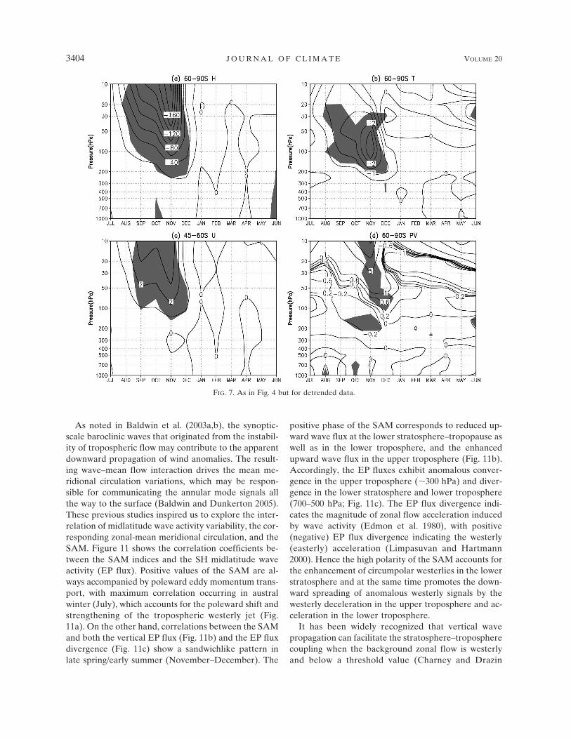
So far, our analyses and calculations have been allbased on the original data. As the apparent linear cor-relation of two variables may be strong by virtue of theshared trends (Thompson et al. 2000), we detrendedboth the SAODI and various physical variables andrecalculated their regression coefficients (Fig. 7) andcorrelation coefficients (Fig. 8). The similarity betweenpatterns in Fig. 4 and Fig. 7 testifies to the robustness ofthe previous statistical analyses. Nevertheless, there arediscrepancies: detrended significant variations occur al-most simultaneously with Antarctic ozone destructionin September–November rather than in a much broadertime window from September to January, as diagnosedfrom the original data (Fig. 4). However, the spatialpatterns of detrended correlation coefficients betweentemperature and the SAODI (Figs. 8a,b) as well as be-tween PV and the SAODI (Figs. 8c,d) are all consistentwith that of the original correlation (Fig. 5). This con-firms the prolonged response of stratospheric circula-tion to the spring Antarctic ozone depletion in early

FIG. 3. (a) Linear trends of Antarctic (60°–90°S) total columnozone during 1980–99 [unit: 10�3 kg m�2 (20 yr)�1]; (b) theSAODI time series (solid line) and its linear trend (dashed line).

3400 J O U R N A L O F C L I M A T E VOLUME 20

summer (December). Besides, the significant negativecorrelation between the SAODI and upward EP fluxstill exists in the lower stratosphere (August) and neartropopause (October and February), even though thetrends are subtracted from both (Fig. 6c). This impliesan ozone–eddy flux interaction process: Interannually,reduced upward eddy flux (and thus the poleward eddyheat flux) in early spring (August) contributes to thespring Antarctic ozone decline because a reduced pole-ward eddy heat flux favors a severe ozone depletion bythe colder temperature. The Antarctic ozone depletion,in turn, causes a reduced midlatitude vertical EP flux inOctober and February. As Hu and Tung (2003)showed, decreasing upward wave activity is related tothe enhancement of the equatorward wave reflection,and less eddy dynamical heating resulting from morewave refraction can be inferred as a component of theozone-related feedback loop.

Now the ozone dynamics in the lower stratospherecan be roughly described as follows: the extraordinary

spring Antarctic ozone depletion originates from thecombined effect of human-released chemicals and thereduced upward wave flux in early spring. Then ozonedepletion induces the intensification, stabilization, andcooling of the polar vortex with enhanced meridionalgradients of PV and temperature between low and highlatitudes, which further isolate the polar vortex and ac-celerate the circumpolar westerlies. At the same time,the strengthening of PV gradients vertically and hori-zontally refract more waves equatorward and down-ward to the troposphere, thus less dynamical heatingand lower temperature in the lower stratosphere. Inaddition, the upward tropospheric eddy flux diminishesin accordance with the severe ozone depletion, result-ing in less wave disturbances to the lower stratosphereand decreased poleward heat flux. This further favors acolder and more stable Antarctic polar vortex. The en-hanced cooling renders the stratospheric ozone layermore susceptible to ozone-destroying chemicals (Aus-tin et al. 1992; Shindell et al. 1998), hence more severe

FIG. 4. Lag-regression coefficients on normalized SAODI. (a) Antarctic (60°–90°S) geopotential height (unit: m); (b)Antarctic air temperature (unit: K); (c) midlatitude (45°–60°S) zonal-mean zonal wind (unit: m s�1); and (d) Antarctic PV(contour intervals: �15, �10, �5, �1, �0.6, �0.2, 0, 0.2, 0.6, 1, 5, 10, 15; unit: IPV, 1 IPV�10�6 K kg�1 m2 s�1). Shadingdenotes areas above the 95% significance level t test.

15 JULY 2007 Y A N G E T A L . 3401

ozone loss. This positive feedback contributes to thepersistence of spring Antarctic ozone depletion andmay be connected to the ozone-related long-termtrends in austral summer.

Clear evidence of this idea can be found through thelinear trend calculations (Fig. 9). Over the past twodecades, the lower-stratosphere polar vortex hasstrengthened (Fig. 9a) and cooled (Fig. 9b), the mid-latitude westerly has accelerated (Fig. 9c), and 100-hPaAntarctic PV has increased (Fig. 9d). All of thesetrends are significant above the 95% confidence level inaustral summer following the spring Antarctic ozonedepletion, except that 200-hPa Antarctic PV (Fig. 9d)exhibits the significant downward trend in a ratherbroad time window from August to February. Besides,the Antarctic tropospheric temperature (Fig. 9b) hasstrong positive trends in winter and spring, which isassumed to be associated with greenhouse gas warming.The stratospheric trends tend to propagate downwardto the lower troposphere, and the surface trends are

significant in January only (Figs. 9a,c). The seasonalityand structure of the 21-yr linear trend pattern of geo-potential height (Fig. 9a) and temperature (Fig. 9b) aresimilar to that of the 30-yr observational trend patternin TS02 (their Fig. 1) with a small discrepancy existingin the geopotential height amplitude.

Note that the linear trends of vertical EP flux exhibitthe suppressed upward wave flux in the troposphereand increased upward wave flux in the lower strato-sphere (Fig. 6d). Obviously, the correlation pattern(Figs. 6b,c) does support the consistency of springozone depletion with EP flux trends in the troposphere,but not in the lower stratosphere (the interannual cor-relation coefficients are not significant in the lowerstratosphere). As the upward EP flux trends in the tro-posphere appear significant in austral winter and spring(June–November), it seems that the reduced tropo-spheric wave forcing trends lead the ozone depletionand then should have great dynamical effects on theozone concentration. However, the lower-stratospheric

FIG. 5. Correlation between SAODI and zonal mean temperature during (a) November and (b) December. Correlationbetween SAODI and potential vorticity during (c) November and (d) December. Shading denotes areas above the 95%significance level t test.

3402 J O U R N A L O F C L I M A T E VOLUME 20

EP flux trends are independent of ozone dynamics, andthe cause and effects of this phenomenon deserve moredetailed investigation.

c. The stratosphere–troposphere coupling anddownward propagation of lower-stratosphericanomalies

So far, we have depicted a positive feedback processin the lower stratosphere associated with spring Ant-arctic ozone depletion. Since our major interest is tofind out how such anomalies can affect the sea levelwind stress, we want to identify dynamical processesresponsible for conveying these perturbations down-ward, that is, processes that generate the nonlocal ef-fects of stratospheric ozone depletion. A potential can-didate responsible for signal transport is the strato-sphere–troposphere dynamical coupling.

It has been recognized that planetary Rossby wavesgenerated in the troposphere can propagate upward.When their amplitude grows large enough, they break;

their energy is absorbed and thus changes the strato-spheric flow. The stratospheric flow, in turn, can affectthe troposphere by downward wave refraction. Existingevidence indicates that the stratosphere–troposphereinteraction processes can project onto the SouthernAnnular Mode in its active season (Thompson et al.2000; Thompson and Solomon 2002; Thompson et al.2005; Kushner and Polvani 2004). Accordingly, we con-struct 18-level SAM indices using ERA-40 monthlygeopotential height data and investigate the downwardpropagation of zonal wind anomalies.

The SAM variabilities associated with the SAODIand its trends are shown in Fig. 10. Obviously, the de-crease in Antarctic ozone concentration corresponds tothe high polarity of SAM indices in the spring and sum-mer stratosphere (Fig. 10a), and the SAM trends arestrong and statistically significant in summer followingthe spring ozone depletion (Fig. 10c). Accordingly, theinterannual correlations are largely reduced in summer,when the trends are subtracted from the ozone andSAM (Fig. 10b).

FIG. 6. (a) 30°–60°S vertical EP flux climatology; (b) correlation between 30°–60°S vertical EP flux and SAODI; (c) asin (b) but for detrended data; and (d) linear trends of 30°–60°S vertical EP flux. Shading denotes areas above the 95%significance level t test.

15 JULY 2007 Y A N G E T A L . 3403

As noted in Baldwin et al. (2003a,b), the synoptic-scale baroclinic waves that originated from the instabil-ity of tropospheric flow may contribute to the apparentdownward propagation of wind anomalies. The result-ing wave–mean flow interaction drives the mean me-ridional circulation variations, which may be respon-sible for communicating the annular mode signals allthe way to the surface (Baldwin and Dunkerton 2005).These previous studies inspired us to explore the inter-relation of midlatitude wave activity variability, the cor-responding zonal-mean meridional circulation, and theSAM. Figure 11 shows the correlation coefficients be-tween the SAM indices and the SH midlatitude waveactivity (EP flux). Positive values of the SAM are al-ways accompanied by poleward eddy momentum trans-port, with maximum correlation occurring in australwinter (July), which accounts for the poleward shift andstrengthening of the tropospheric westerly jet (Fig.11a). On the other hand, correlations between the SAMand both the vertical EP flux (Fig. 11b) and the EP fluxdivergence (Fig. 11c) show a sandwichlike pattern inlate spring/early summer (November–December). The

positive phase of the SAM corresponds to reduced up-ward wave flux at the lower stratosphere–tropopause aswell as in the lower troposphere, and the enhancedupward wave flux in the upper troposphere (Fig. 11b).Accordingly, the EP fluxes exhibit anomalous conver-gence in the upper troposphere (�300 hPa) and diver-gence in the lower stratosphere and lower troposphere(700–500 hPa; Fig. 11c). The EP flux divergence indi-cates the magnitude of zonal flow acceleration inducedby wave activity (Edmon et al. 1980), with positive(negative) EP flux divergence indicating the westerly(easterly) acceleration (Limpasuvan and Hartmann2000). Hence the high polarity of the SAM accounts forthe enhancement of circumpolar westerlies in the lowerstratosphere and at the same time promotes the down-ward spreading of anomalous westerly signals by thewesterly deceleration in the upper troposphere and ac-celeration in the lower troposphere.

It has been widely recognized that vertical wavepropagation can facilitate the stratosphere–tropospherecoupling when the background zonal flow is westerlyand below a threshold value (Charney and Drazin

FIG. 7. As in Fig. 4 but for detrended data.

3404 J O U R N A L O F C L I M A T E VOLUME 20

1961). This condition is met in the SH late spring/earlysummer when the polar vortex decays and when it isbuilding up in the fall (Thompson and Solomon 2002).On account of the strong seasonality of the strato-sphere–troposphere coupling and the lower-strato-spheric circulation, we choose late spring/early summer(October–January) and present the zonal-mean meridi-onal sections of eddy forcing (Fig. 12) and zonal-meanmeridional circulation (Fig. 13) so as to ascertain thedownward propagation of SAM-related zonal-windanomalies. The late spring season (October–Novem-ber) is characterized by prominent dipole patterns ofEP flux divergence at midlatitudes (30°–60°S). Theeddy fluxes converge at �300 hPa and diverge at �500hPa, relaying the strong lower-stratospheric zonal-windanomalies to the middle troposphere (Figs. 12a,b). Inearly summer (December–January), although the up-per-level EP flux convergence diminishes to a large ex-tent, the EP flux divergence at �500 hPa persists, sus-taining the strengthening of westerly wind at this level(Figs. 12c,d). On the other hand, the meridional Ferrelcell strengthens and shifts poleward in accordance with

the positive phase of the SAM (vectors in Fig. 13). Byvirtue of the Coriolis force, the upper (lower-)-levelbranch of the Ferrel cell, that is, the anomalous south-erly (northerly) winds, turns left to decelerate (acceler-ate) the anomalous westerlies, hence facilitating thedownward propagation of westerly anomalies. At thesame time, due to the SAM-related eddy momentumtransport (Fig. 11a), the tropospheric westerly jet shiftspoleward. The resulting coalescence of the tropo-spheric jet with the stratospheric polar night jet en-hances the stratosphere–troposphere coupling andslows propagation of anomalous westerlies, thus col-laborating to convey the SAM zonal-wind signals downto the surface, indicated by the downward shift of con-tours between October and January in Fig. 13.

4. Conclusions and discussion

Through a series of thermodynamical and dynamicalinteractions, the anthropogenic-induced spring Antarc-tic ozone depletion drives the decadal changes in thelower stratosphere and tropopause at the Southern

FIG. 8. As in Fig. 5 but for detrended data.

15 JULY 2007 Y A N G E T A L . 3405

Hemisphere high and midlatitudes, as well as the highpolarity of SAM in the austral spring and summer sea-sons. The stratosphere–troposphere coupling occursduring late spring–early summer by virtue of the SAMmode, resulting in the downward propagation of lower-stratospheric wind anomalies to the troposphere. It is

the synergistic effect of SAM-related wave–mean flowinteraction and anomalous mean meridional circulationthat relays the wind anomaly signals and hereby trig-gers the positive trend of wind stress over the SouthernOcean.

The large-scale upper-level PV anomalies induce

FIG. 10. (a) Lag-regression coefficients of SAM indices on SAODI; (b) as in (a) but for detrended data; and (c) linear trends ofSAM indices for the period 1980–2000. Shading denotes areas above the 95% significance level t test.

FIG. 9. As in Fig. 4 but for linear trends during the period of 1980–2000. [PV contour intervals in (d): �40, �30, �20,�10, �5, �3, �2, �1, 0, 1, 2, 3, 5, 10, 20, 30, 40.]

3406 J O U R N A L O F C L I M A T E VOLUME 20

strong wind fields that can be detected at the ground.By the method of piecewise potential vorticity inver-sion, both Hartley et al. (1998) and Black (2002) upholdthe stratospheric downward forcing of tropospheric cli-

mate variability. Perlwitz and Harnik (2004), on theother hand, suggest that the downward reflection ofwaves is an important component of troposphere–stratosphere dynamics. Our analyses manifest the indi-

FIG. 12. Zonal-mean meridional sections of total EP fluxes (vector: the vertical component is multiplied by 200) and itsdivergences (contour) corresponding to one standard deviation of SAM indices. Shading denotes areas where the EP fluxdivergences are above the 95% significance level t test.

FIG. 11. Correlation between SAM indices and midlatitude (30°–60°S) EP flux: (a) the meridional EP flux; (b) the vertical EP flux;and (c) the EP flux divergence. Shading denotes areas above the 95% significance level t test.

15 JULY 2007 Y A N G E T A L . 3407

rect downward control of lower-stratospheric Antarcticozone depletion on the Southern Ocean surface windstress on decadal time scales. The ozone-related posi-tive feedback influences the lower-stratospheric circu-lation and changes the tropospheric circulation throughwave refraction, thus facilitating the stratosphere–troposphere coupling and downward propagation ofzonal wind anomalies. This adds to the increasing num-ber of studies (e.g., Baldwin et al. 2003b; Scott andPolvani 2004) that support the stratosphere as an activeplayer in the stratosphere–troposphere interaction andthereby global climate changes.

Greenhouse gases (GHGs) have long been viewed asa principal factor driving climate changes (e.g., Fyfe etal. 1999; Kushner et al. 2001; Cai et al. 2003). The SouthPole CO2 monthly data (Fig. 1g) takes on a monotonicupward trend, and this linear trend persists for thewhole 50-yr period in contrast to other time series.However, the seasonality and occurring period of

Southern Ocean wind stress trends are highly coherentwith the Antarctic ozone content. This implicates thatat least in SH mid and high latitudes, the ozone holeplays a more important role than GHGs in driving therecent decadal variabilities, though their synergistic in-teractions should not be neglected (Hartmann et al.2000; Shindell et al. 1998; Shindell and Schmidt 2004).

The importance of surface wind stress over theSouthern Ocean in propelling the Antarctic Circumpo-lar Current (ACC) has been firmly established (Gnan-adesikan and Hallberg 2000; Tansley and Marshall2001; Borowski et al. 2002). Given the unique charac-teristics of ACC (zonally unblocked and huge transportcapacity), the decadal change of the wind stress fieldwill undoubtedly lead to considerable changes in theglobal ocean circulation.

Our discussion has been focused on the atmosphericdynamics; however, large-scale air–sea interaction inthe Southern Ocean may also contribute to global cli-

FIG. 13. Zonal-mean meridional circulation (vector: the vertical velocity is multiplied by 100) and zonal wind (contour)corresponding to one standard deviation of SAM indices. Shading denotes areas where the zonal wind anomalies areabove the 95% significance level t test.

3408 J O U R N A L O F C L I M A T E VOLUME 20

mate changes. In particular, Antarctic IntermediateWater (AAIW) outcrops near the polar front wherestrong air–sea heat and momentum exchanges takeplace. In fact, recently reported Southern Ocean long-term variability associated with AAIW temperatureand salinity property changes (e.g., Gille 2002) may beattributed to climate variabilities at its outcrop region.Changes in sea surface temperature and sea level windstress may interact through complicated air–sea cou-pling mechanisms that, in turn, leads to the SH climatechanges. Scientists have attempted to explore theocean–atmospheric interaction in the Southern Ocean.Hall and Visbeck (2002) simulated the synchronousSouthern Ocean changes corresponding to SAM. Okeand England (2004) presented the oceanic response tothe latitudinal shifts of the subpolar westerly winds.More recently, Cai (2006) associated the southwardshift and spinup of the supergyre in the Southern Oceanwith surface wind changes induced by Antarctic ozonedepletion. But the physical processes of the SouthernOcean in response to these ozone-induced changes maybe far more complicated than commonly assumed.Thus, further inquiry of these processes may be pivotalto our comprehension of long-term ocean circulationand climate changes.

Acknowledgments. This study was supported byMOST of China (Grant 2006CB403604) and ChineseAcademy of Sciences (Grant KZSW2-YW-214) (forYXY and DXW) and W. Alan Clark Chair fromWoods Hole Oceanographic Institution (for RXH).Comments from the reviewers were very helpful inclearing up the presentation. The authors wish to thankDr. Jason Goodman for his help in improving the qual-ity of this manuscript and insightful comments. Discus-sions with Dr. Guihua Wang are much appreciated.

REFERENCES

Albritton, D. L., P. J. Aucamp, G. Megie, and R. T. Watson, 1998:Scientific Assessment of Ozone Depletion: 1998. GlobalOzone Research and Monitoring Project, Rep. 44, WorldMeteorological Organization.

Appenzeller, C., and H. C. Davies, 1992: Structure of strato-spheric intrusions into the troposphere. Nature, 358, 570–572.

Appenzeller, E., J. R. Holton, and K. Rosenlof, 1996: Seasonalvariation of mass transport across the tropopause. J. Geo-phys. Res., 101, 15 701–15 708.

Austin, J., N. Butchart, and K. Shine, 1992: Possibility of an Arcticozone hole in a doubled-CO2 climate. Nature, 360, 221–225.

Baldwin, M. P., and T. J. Dunkerton, 2005: The solar cycle andstratosphere- troposphere dynamical coupling. J. Atmos. Sol.-Terr. Phys., 67, 71–82.

——, D. B. Stephenson, D. W. J. Thompson, T. J. Dunkerton,A. J. Charlton, and A. O’Neill, 2003a: Stratospheric memoryand extended-range weather forecasts. Science, 301, 636–640.

——, D. W. J. Thompson, E. F. Shuckburgh, W. A. Norton, andN. P. Gillett, 2003b: Weather from the stratosphere? Science,301, 317–319.

Bengtsson, L., K. I. Hodges, and S. Hagemann, 2004: Sensitivity ofthe ERA40 reanalysis to the observing system: Determina-tion of the global atmospheric circulation from reduced ob-servations. Tellus, 56A, 456–471.

Black, R. X., 2002: Stratospheric forcing of surface climate in theArctic Oscillation. J. Climate, 15, 268–277.

Borowski, D., R. Gerdes, and D. Olbers, 2002: Thermohaline andwind forcing of a circumpolar channel with blocked geo-strophic contours. J. Phys. Oceanogr., 32, 2520–2540.

Cai, W., 2006: Antarctic ozone depletion causes an intensificationof the Southern Ocean super-gyre circulation. Geophys. Res.Lett., 33, L03712, doi:10.1029/2005GL024911.

——, P. H. Whetton, and D. J. Karoly, 2003: The response of theAntarctic Oscillation to increasing and stabilized atmosphericCO2. J. Climate, 16, 1525–1538.

Charney, J. G., and P. G. Drazin, 1961: Propagation of planetary-scale disturbances from the lower into the upper atmosphere.J. Geophys. Res., 66, 83–109.

Chung, C., and S. Nigam, 1999: Weighting of geophysical data inPrincipal Component Analysis. J. Geophys. Res., 104, 16 925–16 928.

Crutzen, P. J., and F. Arnold, 1986: Nitric-acid cloud formation inthe cold Antarctic stratosphere: A major cause for the spring-time ozone hole. Nature, 324, 651–655.

Edmon, H. J., Jr., B. J. Hoskins, and M. E. McIntyre, 1980: Elias-sen–Palm cross sections for the troposphere. J. Atmos. Sci.,37, 2600–2616.

Farman, J. C., B. G. Gardiner, and J. D. Shankin, 1985: Largelosses of total ozone in Antarctica reveal ClOX/NOX inter-action. Nature, 315, 207–210.

Fyfe, J. C., G. J. Boer, and G. M. Flato, 1999: The Arctic andAntarctic oscillations and their projected change underglobal warming. Geophys. Res. Lett., 26, 1601–1604.

Garratt, J. R., 1977: Review of drag coefficients over oceans andcontinents. Mon. Wea. Rev., 105, 915–929.

Gille, S. T., 2002: Warming of the Southern Ocean since the 1950s.Science, 295, 1275–1277.

Gillett, N. P., and D. W. J. Thompson, 2003: Simulation of recentSouthern Hemisphere climate change. Science, 302, 273–275.

Gnanadesikan, A., and R. W. Hallberg, 2000: On the relationshipof the circumpolar current to the Southern Hemispherewinds in the coarse-resolution ocean models. J. Phys. Ocean-ogr., 30, 2013–2034.

Hall, A., and M. Visbeck, 2002: Synchronous variability in theSouthern Hemisphere atmosphere, sea ice, and ocean result-ing from the Annular Mode. J. Climate, 15, 3043–3057.

Hartley, D. E., J. Villarin, R. X. Black, and C. A. Davis, 1998: Anew perspective on the dynamical link between the strato-sphere and troposphere. Nature, 391, 471–474.

Hartmann, D. L., J. M. Wallace, V. Limpasuvan, D. W. J. Thomp-son, and J. R. Holton, 2000: Can ozone depletion and globalwarming interact to produce rapid climate change? Proc.Natl. Acad. Sci. USA, 92, 1412–1417.

Hines, K. M., D. H. Bromwich, and G. J. Marshall, 2000: Artificialsurface pressure trends in the NCEP–NCAR reanalysis overthe Southern Ocean and Antarctica. J. Climate, 13, 3940–3952.

Holton, J. R., P. H. Haynes, M. E. McIntyre, A. R. Douglass,R. B. Rood, and L. Pfister, 1995: Stratosphere-troposphereexchange. Rev. Geophys., 33, 403–439.

15 JULY 2007 Y A N G E T A L . 3409

Hood, L. L., and B. E. Soukharev, 2005: Interannual variations oftotal ozone at northern midlatitudes correlated with strato-spheric EP flux and potential vorticity. J. Atmos. Sci., 62,3724–3739.

Hoskins, B. J., 1991: Towards a PV-� view of the general circula-tion. Tellus, 43AB, 27–35.

——, M. E. McIntyre, and A. W. Robertson, 1985: On the use andsignificance of isentropic potential vorticity maps. Quart. J.Roy. Meteor. Soc., 111, 877–946.

Hu, Y. Y., and K. K. Tung, 2003: Possible ozone-induced long-term changes in planetary wave activity in late winter. J. Cli-mate, 16, 3027–3038.

Huang, R. X., 1998: On the balance of energy in the oceanic gen-eral circulation. Chin. J. Atmos. Sci, 22, 452–467.

——, 2004: Ocean, energy flow. Encyclopedia of Energy, C. J.Cleveland, Ed., Vol. 4, Elsevier, 497–509.

——, W. Wang, and L. L. Liu, 2006: Decadal variability of windenergy input to the world ocean. Deep-Sea Res. II, 53, 31–41.

Kallberg, P., A. Simmons, S. Uppala, and M. Fuentes, 2004: TheERA-40 archive. ERA-40 Project Report Series No. 17,35 pp.

Kushner, P. J., and L. M. Polvani, 2004: Stratosphere–tropospherecoupling in a relatively simple AGCM: The role of eddies. J.Climate, 17, 629–639.

——, I. M. Held, and T. L. Delworth, 2001: Southern Hemisphereatmospheric circulation response to global warming. J. Cli-mate, 14, 2238–2249.

Langematz, U., 2000: An estimate of the impact of observedozone losses on stratospheric temperature. Geophys. Res.Lett., 27, 2077–2080.

Limpasuvan, V., and D. L. Hartmann, 2000: Wave-maintained an-nular modes of climate variability. J. Climate, 13, 4414–4429.

Mahlmann, R. D., J. P. Pinto, and L. J. Umscheid, 1994: Trans-port, radiative, and dynamical effects of the Antarctic ozonehole: A GFDL “SKYHI” model experiment. J. Atmos. Sci.,51, 489–509.

Marshall, G. J., 2002: Trends in Antarctic geopotential height andtemperature: A comparison between radiosonde and NCEP–NCAR reanalysis data. J. Climate, 15, 659–674.

——, 2003: Trends in the southern annular mode from observa-tions and reanalyses. J. Climate, 16, 4134–4143.

McElroy, M. B., R. J. Salawitch, S. C. Wofsy, and J. A. Logan,1986: Reductions of Antarctic ozone due to synergistic inter-actions of chlorine and bromine. Nature, 321, 759–762.

McIntyre, M. E., and T. N. Palmer, 1984: The “surf zone” in thestratosphere. J. Atmos. Terr. Phys., 46, 825–849.

Nakamura, M., and R. A. Plumb, 1994: The effects of flow asym-metry on the direction of Rossby wave breaking. J. Atmos.Sci., 51, 2031–2045.

Oke, P. R., and M. H. England, 2004: Ocean response to changesin the latitude of the Southern Hemisphere subpolar westerlywinds. J. Climate, 17, 1040–1054.

Perlwitz, J., and N. Harnik, 2004: Downward coupling betweenthe stratosphere and troposphere: The relative roles of waveand zonal mean processes. J. Climate, 17, 4902–4909.

Polstel, G. A., and M. H. Hitchman, 1999: A climatology ofRossby wave breaking along the subtropical tropopause. J.Atmos. Sci., 56, 359–373.

Polvani, L. M., and D. W. Waugh, 2004: Upward wave activityflux as a precursor to extreme stratospheric events and sub-sequent anomalous surface weather regimes. J. Climate, 17,3548–3554.

Ramaswamy, V., and Coauthors, 2001: Stratospheric temperaturetrends: Observations and model simulations. Rev. Geophys.,39, 71–122.

Randel, W. J., and F. Wu, 1999: Cooling of the Arctic and Ant-arctic polar stratospheres due to ozone depletion. J. Climate,12, 1467–1479.

Santer, B. D., T. M. L. Wigley, J. S. Boyle, D. J. Gaffen, J. J.Hnilo, D. Nychka, D. E. Parker, and K. E. Taylor, 2000: Sta-tistical significance of trends and trend differences in layer-average atmospheric temperature time series. J. Geophys.Res., 105, 7337–7356.

Scott, R. K., and L. M. Polvani, 2004: Stratospheric control ofupward wave flux near the tropopause. Geophys. Res. Lett.,31, L02115, doi:10.1029/2003GL017965.

Shindell, D. T., and G. A. Schmidt, 2004: Southern Hemisphereclimate response to ozone changes and greenhouse gas in-creases. Geophys. Res. Lett., 31, L18209, doi:10.1029/2004GL020724.

——, D. Rind, and P. Lonergan, 1998: Increased polar strato-spheric ozone losses and delayed eventual recovery due toincreasing greenhouse gas concentrations. Nature, 392, 589–592.

Shine, K. P., 1986: On the modeled thermal response of the Ant-arctic stratosphere to a depletion of ozone. Geophys. Res.Lett., 13, 1331–1334.

Solomon, S., 1999: Stratospheric ozone depletion: A review ofconcepts and history. Rev. Geophys., 37, 275–316.

——, R. R. Garcia, F. S. Rowland, and D. J. Wuebbles, 1986: Onthe depletion of Antarctic ozone. Nature, 321, 755–758.

Stolarski, R. S., A. J. Krueger, M. R. Schoeberl, R. D. McPeters,P. A. Newman, and J. C. Alpert, 1986: Nimbus-7 satellitemeasurements of the springtime Antarctic ozone decrease.Nature, 322, 808–811.

Tansley, C. E., and D. P. Marshall, 2001: On the dynamics ofwind-driven circumpolar currents. J. Phys. Oceanogr., 31,3258–3273.

Thompson, D. W. J., and S. Solomon, 2002: Interpretation ofrecent Southern Hemisphere climate change. Science, 296,895–899.

——, J. M. Wallace, and G. C. Hegerl, 2000: Annular modes in theextratropical circulation. Part II: Trends. J. Climate, 13, 1018–1036.

——, M. P. Baldwin, and S. Solomon, 2005: Stratosphere–troposphere coupling in the Southern Hemisphere. J. Atmos.Sci., 62, 708–715.

Waugh, D. W., W. J. Randel, S. Pawson, P. A. Newman, and E. R.Nash, 1999: Persistence of the lower stratospheric polar vor-tices. J. Geophys. Res., 104, 27 191–27 201.

Wunsch, C., and R. Ferrari, 2004: Vertical mixing, energy, and thegeneral circulation of the oceans. Annu. Rev. Fluid Mech., 36,281–314.

Zhou, S., M. E. Gelman, A. J. Miller, and J. P. McCormack, 2000:An inter-hemisphere comparison of the persistent strato-spheric polar vortex. Geophys. Res. Lett., 27, 1123–1126.

3410 J O U R N A L O F C L I M A T E VOLUME 20