Waste disposal practice of urban dwellers: A Study on Khulna City
Upload
chloe-mathewsCategory
view
220download
0
DDSS2006
A Comparison Study about the Allocation Problem of Undesirable Facilities Based on Residential Awareness
– A Case Study on Waste Disposal Facility in ChengDu City, Sichuan China –
K. Zhou, A. Kondo, A.Cartagena Gordillo1 and K. WatanabeThe University of Tokushima, Tokushima, Japan 1Yokohama National University, Yokohama, Japan

2
Motivation I
• In the existing facility location theory, there are many studies concerned with location modeling of facilities that put more importance on nearness. But there are also some facilities that give undesirable feeling to residents. Location problems for those kind of facilities require new methodologies with corresponding solutions.
• Thereupon, in this research, our purpose is to consider the location problem of undesirable facilities
• Waste disposal facilities are appointed for analysis. Specifically, we choose garbage transfer stations and final disposal facilities as research objects due to their high level of variety.
2

3
Motivation II
• As we review the methodologies for location problems of undesirable facility, we found that the most popular way of handling undesirability for a single facility is to minimize the highest effect on a series of fixed points applying the principle of locating the undesirable facilities as far as possible from all sensitive places.
• Therefore, in the existing literature we can appreciate that physical magnitudes, such as distance or time, were mainly used as important parameters on the study of facility location. However, the psychology element of the facility users was not given enough attention.
• Regarding those characteristic, our objective in this research is to analyze location problems of undesirable facilities by using a model based on probability theory, which considers residential awareness.
3

4
Contents
3-Parameter LoglogisticWeibull Non-Parametric
Regression Analysis Matlab Minitab
Parameters Estimation
Endurance Rate Function
Conclusions
4
Stochastic Methods
Modeling

5
Definition of Endurance Distance & Endurance Rate
For purely undesirable facilities, we can consider that residents hope the undesirable facility can be located farther than a certain distance, which means the residents can endure the location of the undesirable facility if the facility is located farther than that distance. Then the minimum of this desired distance can be defined as endurance distance, which is expressed here as w. And, when an undesirable facility is located at a certain distance, the rate of residents who could endure the facility location is defined as endurance rate, which is expressed here as P(x) in this research.
●
Residential location
Undesirable facility
Endurance distance
W
X > W (X : distance to a facility)
5
6
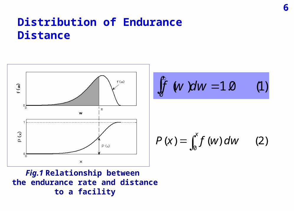
Distribution of Endurance Distance
)1(0.1)(0 dwwf
)2()()(0x
dwwfxP
Fig.1 Relationship between the endurance rate and distance to a facility
6
7
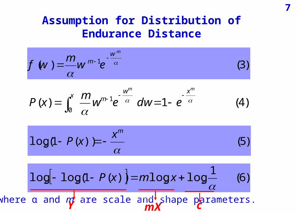
Assumption for Distribution of Endurance Distance
)4(1)(0
1
mm xx
wm edwew
mxP
)3()( 1
mwm ew
mwf
)5())(1(log
m
e
xxP
)6(1
loglog))(1(loglogeeee xmxP
where α and m are scale and shape parameters. Y mX c
7

Survey Concerning Endurance Distance
Estimation of parameters for endurance rate function
Data concerning the endurance rate P(x)
Carry out a questionnaire survey toward the residents in object area
Questionnaire Survey
At least how far should a waste facility be located to your home?
8
9
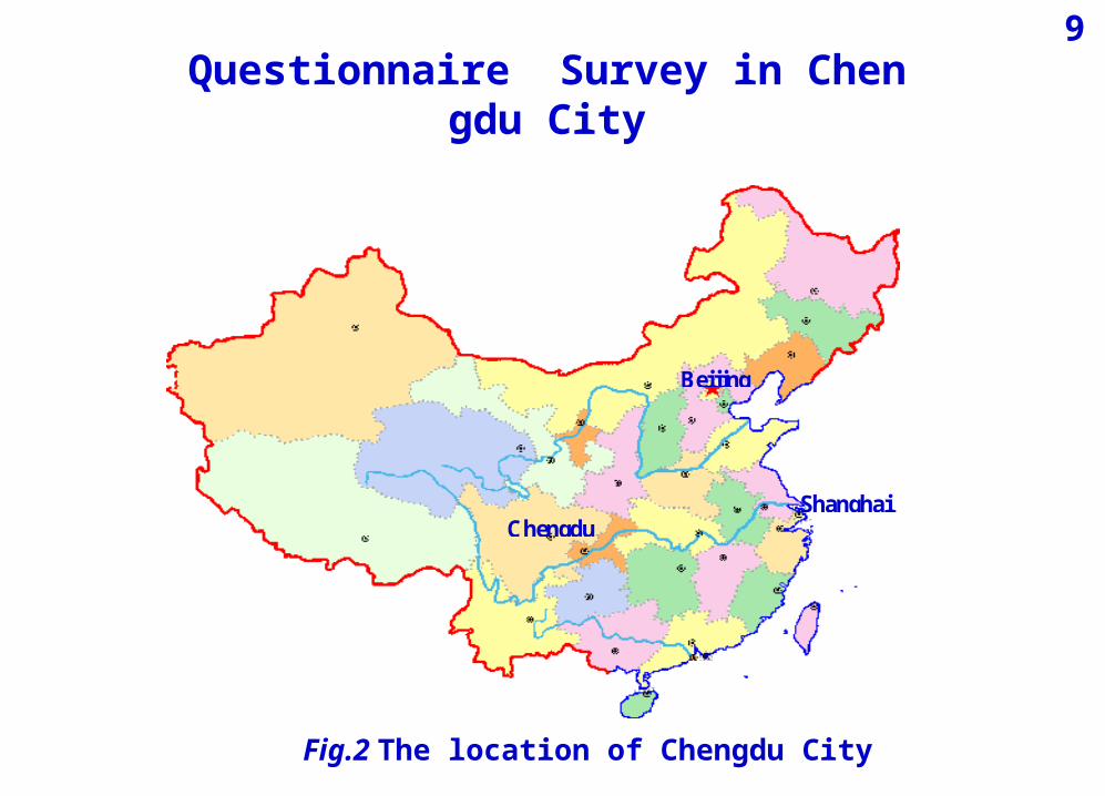
Questionnaire Survey in Chengdu City
Fig.2 The location of Chengdu City
Chengdu
Beijing
Shanghai Chengdu
Beijing
Shanghai
9

10
Case Study Area-object of Survey
― ― :Main Road
― ― :other Road
Survey Area
Fig.3 Object area of the research
10

11
The Result of Survey
11
3 % 4 %
11 %
3 1 %
2 4 %
2 7 %
1 0 's
2 0 's
3 0 's
4 0 's
5 0 's
6 0 's ~
Fig.4
Percentage by age
Distributed survey
Valid answers
Valid response rate
350
323
Percentage by sex
92.3%
male
52%
female
48%

12
18.0
0.3 0.6
44.3
23.5
13.3
0
20
40
60
0~3 4~6 7~9 10~12 13~15 16~Distance (km)
Per
cent
age
of P
eopl
e (%
)
Fig.5
Distance to garbage transfer
stations and corresponding
residential endurance rate
5.6 8.0 6.5
56.7
6.5
12.7
4.00
20
40
60
80
1~5 6~10 11~15 16~20 21~25 20~30 31~
Distance (km)
Per
cent
age
of P
eopl
e (%
)
Fig.6
Distance to final waste disposal facilities and corresponding residential endurance rate
12
Endurance Distance and Endurance Rate

13
Average Endurance Distance Classified by Attribute
5.867.28 7.56 7.83 7.17
9.73
0
3
6
9
12
teens twenties thirties forties fifties sixties andabove
km
Fig.7 Average endurance distance classified by age for garbage transfer stations
25.9329.66
35.08
25.66
32.2727.75
0
10
20
30
40
teens twenties thirties forties fifties sixties andabove
km
Fig.8 Average endurance distance classified by age for final waste disposal facilities
7.42
31.13
7.64
28.58
0
7
14
21
28
35
garbage transfer stations final waste disposal facility
km
male
female
Fig.9 Average endurance distance classified by sex
13

14
Estimated Parameters of Endurance Rate Function
garbage transfer final waste disposal
stations facilities
parameter α 38.7 (9.971) 522.5 (19.312)
parameter m 1.809 (9.383) 1.781 (16.968)
R 2 0.880 0.947numbers of sample 14 18
facilities
Table 1. Result of parameters estimation for the endurance rate model
where the numbers between parentheses represent the value of t.R2 is determination Coefficient
14

15
0
20
40
60
80
100
0 5 10 15 20
Distance (km)
End
uran
ce R
ate
(%)
curve from the model plots from survey data
Fig.10 The residential
endurance rate for garbage transfer stations
0
20
40
60
80
100
0 20 40 60 80Distance (km)
End
uran
ce R
ate
(%)
curve from the model plots from the survey data
Fig.11 The residential
endurance rate for final waste disposal facilities
15

16
NON-PARAMETRIC DISTRIBUTION METHOD
16
In matrix form, non-linear models are given by the formula:
y = f(X, β)+ ε,
where y is an n-by-1 vector of responses, f is a function of β and X, β is a m-by-1 vector of coefficients, X is the n-by-m design matrix for the model, ε is an n-by-1 vector of errors, n is the number of data and m is the number of coefficients.
The fitting process was automated, employing the commercial software Fitting Toolbox from Matlab.

17
Distribution Fitting for Non-parametric Distribution
a1 = 0.0001 a2 = -1.41 a3 = 0.323 a4 = 0.040 a5 = -0.237
b1 = -1.62 b2 = 5.108 b3 =10.00 b4 = 7.935 b5 = 6.962
c1 = 56.90 c2 = 2.364 c3 = 0.682 c4 = 0.565 c5 = 1.628
a6 = 1.541 a7 = -0.222 a8 = 0.067
b6 = 5.359 b7 = -45.73 b8 = 1.015
c6 = 2.599 c7 = 24.950 c8 = 0.744
SSE: 0.0002
R2: 0.9997
RMSE: 0.0012
Table 2. The coefficients of equation (7) and goodness of fit
where, y(x) is probability distribution function (7)2^8/)8((exp(82^7/)7((exp(7
2^6/)6((exp(62^5/)5((exp(52^4/)4((exp(4
2^3/)3((exp(32^2/)2((exp(22^1/)1((exp(1)(
cbxacbxa
cbxacbxacbxa
cbxacbxacbxaxy
17

18
Cumulative Distribution Function Calculation
d1 = 0.64e-1 d2 = 0.44e-1 d3 = -2.96 d4 = 0.195 d5 = 0.2e-1 d6 =-0.342 d7 = 3.549 d8 = -4.91
e1 = 0.18e-1 e2 = 1.344 e3 = 0.423 e4 = 1.466 e5 = 1.770 e6 = 0.614 e7 = 0.385 e8 = 0.401
g1 = 0.28e-1 g2 = -1.364 g3 = -2.161 g4 = -14.66 g5 = -14.04 g6 = -4.28 g7 = -2.06 g8 = 1.833
h1= 5.363
Table 3. The coefficients of equation (8) (with 95% confidence bounds)
1)88(8)77(7)66(6)55(5
)44(4)33(3)22(2)11(1
)()(0
hgeerfdgeerfdgeerfdgeerfd
geerfdgeerfdgeerfdgeerfd
dxxyh
where erf(.) is the error function (8)
18

19
0
20
40
60
80
100
0 2 4 6 8 10 12Distance (km)
End
uran
ce r
ate
(%)
curve from the model plots from survey data
Fig.12 Distribution of the endurance rate h(λ)
19

3-PARAMETER LOGLOGISTIC DISTRIBUTION METHOD
Analysis of Data
_Number of People
Distance_IntervalDensity Coefficient
20
0
50
100
150
0 2 4 6 8 10 12
Distance (km)
Num
ber
of
Peo
ple
Fig.13 A plot of the original data to 12km
21
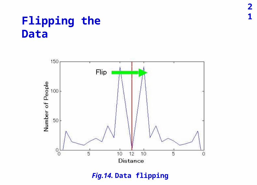
Flipping the Data
Fig.14. Data flipping
21
22
Flipping the Data
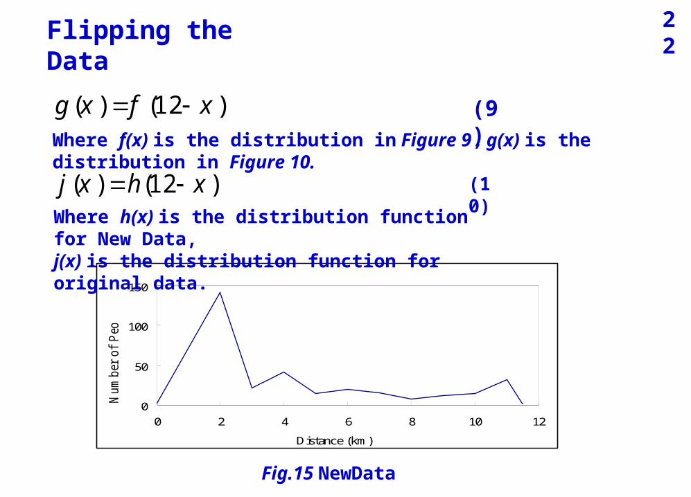
)12()( xfxg (9)
)12()( xhxj (10)
Fig.15 NewData
22
Where f(x) is the distribution in Figure 9 , g(x) is the distribution in Figure 10.
0
50
100
150
0 2 4 6 8 10 12
Distance (km)
Num
ber
of
Peo
ple
Where h(x) is the distribution function for New Data,j(x) is the distribution function for original data.

23
Distribution Analysis of NewData
2)ln(
)ln(
1)(
1)(
b
acx
b
acx
e
e
cxbxh (11)
where, a = Location parameter, b = Scale parameter, c = Threshold parameter
23
Employing the estimation method of Least Squares, a 3-Parameter Loglogistic distribution function was found as:

24
The Resulting Values for the Parameters & the Goodness of Fit
C1 - Threshold
Percent
100101
99.9
99
959080706050403020105
1
0.1
Table of Statistics
StDev 5.16988Median 3.56087IQR 2.95870Failure 320Censor 0
Loc
AD* 0.465Correlation 0.997
1.18332Scale 0.399455Thres 0.295683Mean 4.60651
Probability Plot for C1
Complete Data - LSXY Estimates3- Parameter Loglogistic - 95% CI
Fig.16 Result of parameter estimation and test of goodness of distribution (Where, C1 means NewData shown in Figure 13)
24
a=1.183
b=0.399
c=0.296
25
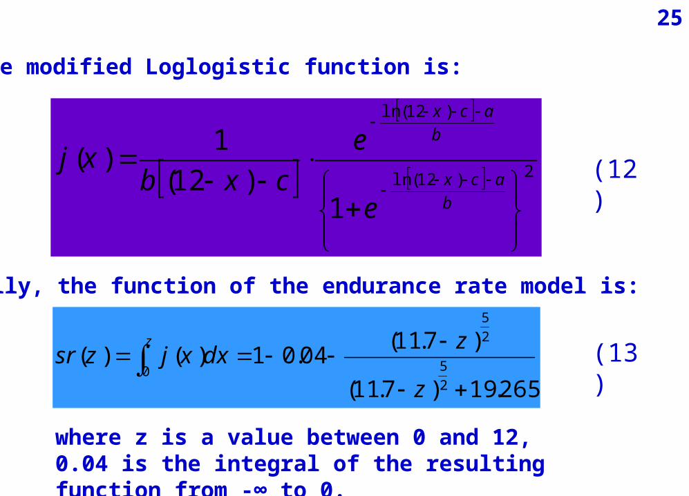
2)12(ln
)12(ln
1)12(
1)(
b
acx
b
acx
e
e
cxbxj
265.19)7.11(
)7.11(04.01)()(
2
5
2
5
0
z
zdxxjzsr
z
(12)
(13)
where z is a value between 0 and 12, 0.04 is the integral of the resulting function from -∞ to 0.
25
The modified Loglogistic function is:
Finally, the function of the endurance rate model is:
26
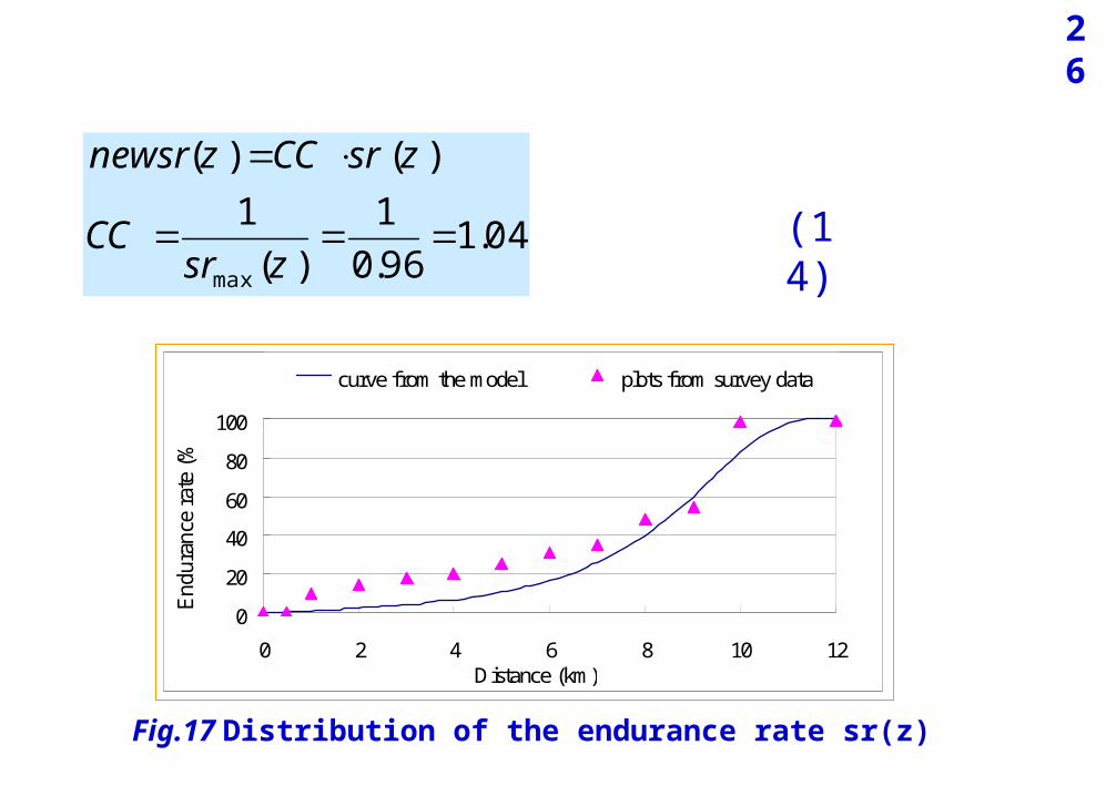
04.196.0
1
)(
1
)()(
max
zsrCC
zsrCCznewsr
(14)
0
20
40
60
80
100
0 2 4 6 8 10 12Distance (km)
En
du
ran
ce r
ate
(%)
curve from the model plots from survey data
Fig.17 Distribution of the endurance rate sr(z)
26
27
CONCLUSIONS
• Regarding undesirable facilities, we defined residential endurance distance and endurance rate, modeled the relationship between facility’s location and the endurance rate.
• From the questionnaire survey carried out in Chengdu City, we could dissect the distribution of residential endurance distance for garbage transfer stations and final waste disposal facility. Using the endurance rate model, we indicated it’s possible to propose waste facilities’ location from the viewpoint of residents.
• Based on different probability distribution functions, we proposed three models for estimating the residential endurance rate and make a comparison study. Based on those models, we found there’s no big difference between the results when residential endurance rate according to facility location is 80%, the calculation results of suitable distance for garbage transfer stations are all around 10km.
• From the comparison study, we found that the advantage of the model employing Weibull distribution is its simplicity; it has only 2 parameters and can be used for the both kinds of facilities though the accuracy was not good enough. The Non-parametric one described a better modelling even though a lot of parameters were needed for describing the detail of the data. As computer technology is developed today, we consider that this method can be used for any kind of situation as a numerical analysis model. Based on a parametric distribution function, we also found a model by analysing and flipping the data as explained above. For this case, the model using Loglogistic distribution function is a new experiment with good modelling characteristics.
27

Thank you for your attention!

質 問 対 策

30
Slide 3
• What’s the meaning of “the highest effect”?
• What are the meaning of “fixed points”?
• What means “a series of fixed points”?
31
Slide 3
• Why need consider residential awareness in this study?

32
Why & how could find Weibull
During the proceeding, we found Weibull distribution has some interesting characters as following: 1. It is a distribution with good elasticity. The shape changes following shape parameter’s changing. 2. The distribution function is completely integrabel, which make it possiblefor next step of parameter estimation.
33
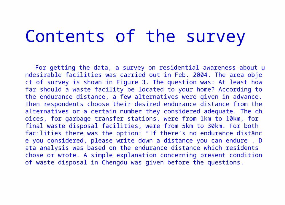
Contents of the survey
For getting the data, a survey on residential awareness about undesirable facilities was carried out in Feb. 2004. The area object of survey is shown in Figure 3. The question was: At least how far should a waste facility be located to your home? According to the endurance distance, a few alternatives were given in advance. Then respondents choose their desired endurance distance from the alternatives or a certain number they considered adequate. The choices, for garbage transfer stations, were from 1km to 10km, for final waste disposal facilities, were from 5km to 30km. For both facilities there was the option: “If there’s no endurance distance you considered, please write down a distance you can endure”. Data analysis was based on the endurance distance which residents chose or wrote. A simple explanation concerning present condition of waste disposal in Chengdu was given before the questions.

34
What means
In matrix form, non-linear models are given by the formula:
y = f(X, β)+ ε,
where y is an n-by-1 vector of responses, f is a function of β and X, β is a m-by-1 vector of coefficients, X is the n-by-m design matrix for the model, ε is an n-by-1 vector of errors, n is the number of data and m is the number of coefficients.
The fitting process was automated, employing the commercial software Fitting Toolbox from Matlab.
35
Table 2
If the value of “goodness of fit” can be gain at the step of distribution fitting?
36
The procedure of selecting equation (11) by employing MINITAB

37
Explaining the following paragraph
The function j(x) in equation (13) exists for values x<0, which is unreal for the processed data, then an adjusting value of 0.04 is included in equation (13) which corresponds to the integral of j(x) from -∞ to 0. For this reason, the endurance rate never reaches 100%. A corrective coefficient can be applied to the equation of the endurance rate sr(z). Then it becomes equation (14). The corrected function newsr(z) is illustrated in Figure 12.