Day Count Conventions: Actual/Actual

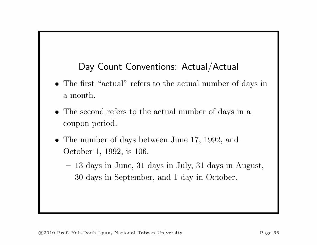
Day Count Conventions: Actual/Actual

• The first “actual” refers to the actual number of days in

a month.

• The second refers to the actual number of days in a

coupon period.

• The number of days between June 17, 1992, and

October 1, 1992, is 106.

– 13 days in June, 31 days in July, 31 days in August,

30 days in September, and 1 day in October.

c⃝2010 Prof. Yuh-Dauh Lyuu, National Taiwan University Page 66

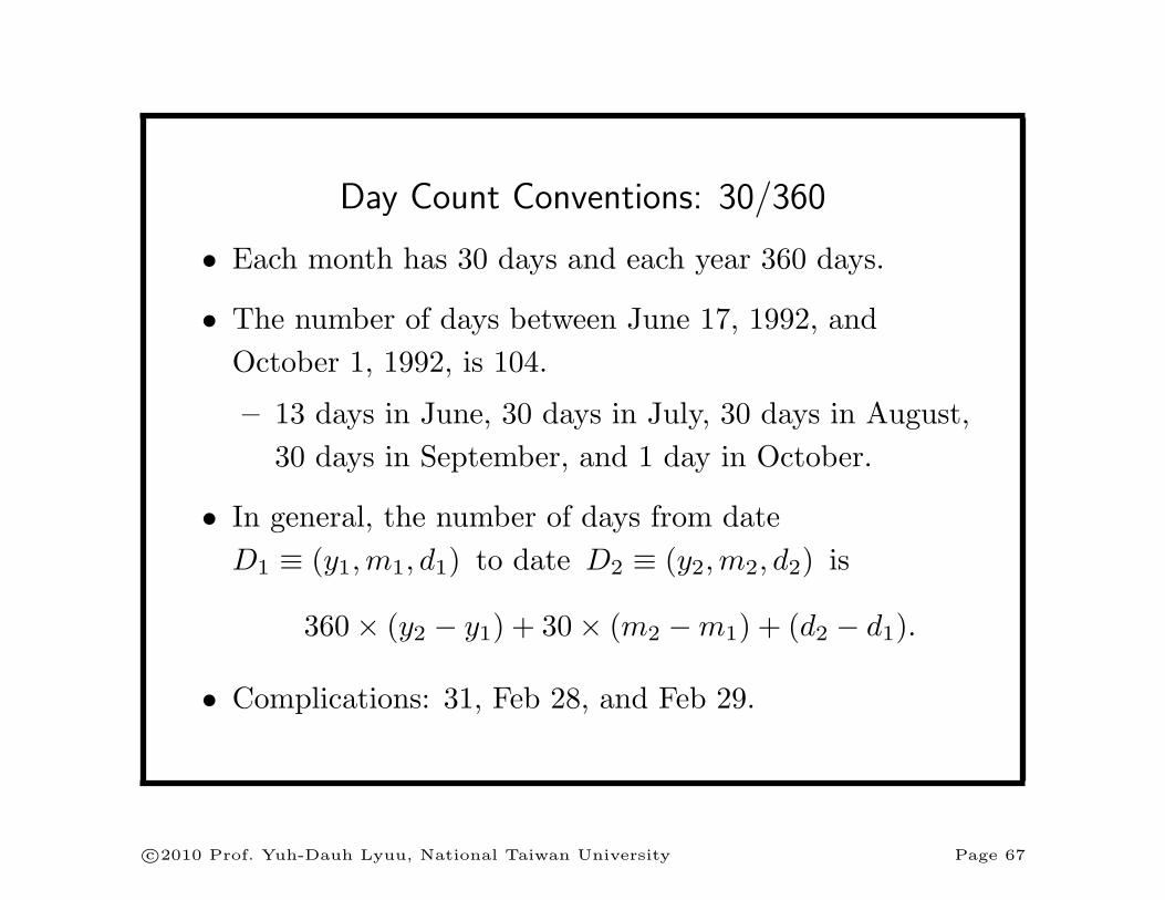
Day Count Conventions: 30/360

• Each month has 30 days and each year 360 days.

• The number of days between June 17, 1992, and

October 1, 1992, is 104.

– 13 days in June, 30 days in July, 30 days in August,

30 days in September, and 1 day in October.

• In general, the number of days from date

D1 ≡ (y1,m1, d1) to date D2 ≡ (y2,m2, d2) is

360× (y2 − y1) + 30× (m2 −m1) + (d2 − d1).

• Complications: 31, Feb 28, and Feb 29.


Full Price (Dirty Price, Invoice Price)

• In reality, the settlement date may fall on any day

between two coupon payment dates.

• Let

ω ≡

number of days between the settlement

and the next coupon payment date

number of days in the coupon period. (6)

• The price is now calculated by

PV =

n−1∑i=0

C(1 + r

m

)ω+i+

F(1 + r

m

)ω+n−1 . (7)


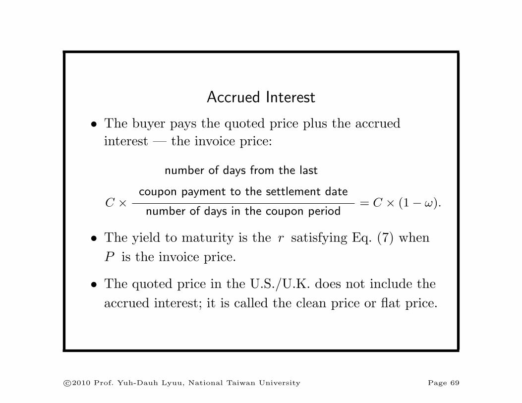
Accrued Interest

• The buyer pays the quoted price plus the accrued

interest — the invoice price:

C ×

number of days from the last

coupon payment to the settlement date

number of days in the coupon period= C × (1− ω).

• The yield to maturity is the r satisfying Eq. (7) when

P is the invoice price.

• The quoted price in the U.S./U.K. does not include the

accrued interest; it is called the clean price or flat price.


-

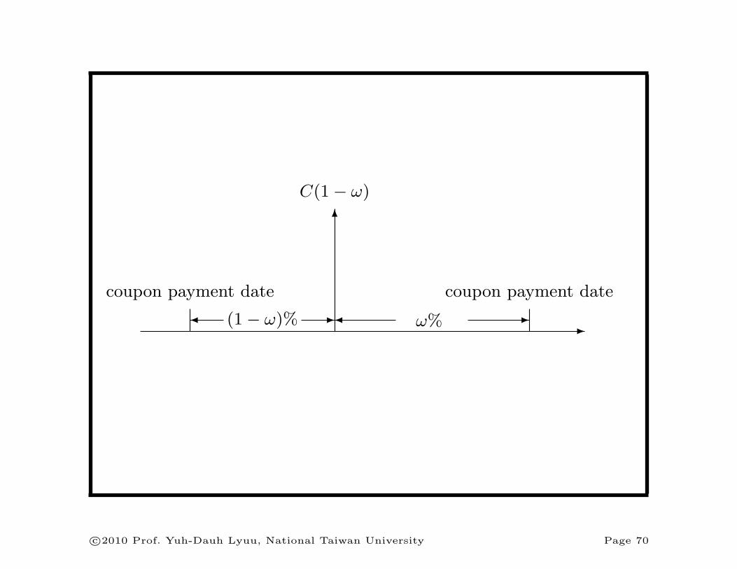
6

coupon payment date

C(1− ω)

coupon payment date

� -(1− ω)% � -ω%


Example (“30/360”)

• A bond with a 10% coupon rate and paying interest

semiannually, with clean price 111.2891.

• The maturity date is March 1, 1995, and the settlement

date is July 1, 1993.

• There are 60 days between July 1, 1993, and the next

coupon date, September 1, 1993.


Example (“30/360”) (concluded)

• The accrued interest is (10/2)× 180−60180 = 3.3333 per

$100 of par value.

• The yield to maturity is 3%.

• This can be verified by Eq. (7) on p. 68 with

– ω = 60/180,

– m = 2,

– C = 5,

– PV= 111.2891 + 3.3333,

– r = 0.03.

c⃝2010 Prof. Yuh-Dauh Lyuu, National Taiwan University 2

Price Behavior (2) Revisited

• Before: A bond selling at par if the yield to maturity

equals the coupon rate.

• But it assumed that the settlement date is on a coupon

payment date.

• Now suppose the settlement date for a bond selling at

par (i.e., the quoted price is equal to the par value) falls

between two coupon payment dates.

• Then its yield to maturity is less than the coupon rate.

– The short reason: Exponential growth is replaced by

linear growth, hence “overpaying” the coupon.


Bond Price Volatility


“Well, Beethoven, what is this?”

— Attributed to Prince Anton Esterhazy


Price Volatility

• Volatility measures how bond prices respond to interest

rate changes.

• It is key to the risk management of interest

rate-sensitive securities.

• Assume level-coupon bonds throughout.


Price Volatility (concluded)

• What is the sensitivity of the percentage price change to

changes in interest rates?

• Define price volatility by

−∂P∂y

P.


Price Volatility of Bonds

• The price volatility of a coupon bond is

−(C/y)n−

(C/y2

) ((1 + y)n+1 − (1 + y)

)− nF

(C/y) ((1 + y)n+1 − (1 + y)) + F (1 + y).

– F is the par value.

– C is the coupon payment per period.

• For bonds without embedded options,

−∂P∂y

P> 0.


Macaulay Duration

• The Macaulay duration (MD) is a weighted average of

the times to an asset’s cash flows.

• The weights are the cash flows’ PVs divided by the

asset’s price.

• Formally,

MD ≡ 1

P

n∑i=1

iCi

(1 + y)i.

• The Macaulay duration, in periods, is equal to

MD = −(1 + y)∂P

∂y

1

P. (8)


MD of Bonds

• The MD of a coupon bond is

MD =1

P

[n∑

i=1

iC

(1 + y)i+

nF

(1 + y)n

]. (9)

• It can be simplified to

MD =c(1 + y) [ (1 + y)n − 1 ] + ny(y − c)

cy [ (1 + y)n − 1 ] + y2,

where c is the period coupon rate.

• The MD of a zero-coupon bond equals its term to

maturity n.

• The MD of a coupon bond is less than its maturity.


Remarks

• Equations (8) on p. 79 and (9) on p. 80 hold only if the

coupon C, the par value F , and the maturity n are all

independent of the yield y.

– That is, if the cash flow is independent of yields.

• To see this point, suppose the market yield declines.

• The MD will be lengthened.

• But for securities whose maturity actually decreases as a

result, the MD (as originally defined) may actually

decrease.


How Not To Think about MD

• The MD has its origin in measuring the length of time a

bond investment is outstanding.

• The MD should be seen mainly as measuring price

volatility.

• Many, if not most, duration-related terminology cannot

be comprehended otherwise.


Conversion

• For the MD to be year-based, modify Eq. (9) on p. 80 to

1

P

[n∑

i=1

i

k

C(1 + y

k

)i + n

k

F(1 + y

k

)n],

where y is the annual yield and k is the compounding

frequency per annum.

• Equation (8) on p. 79 also becomes

MD = −(1 +

y

k

) ∂P

∂y

1

P.

• By definition, MD (in years) =MD (in periods)

k .


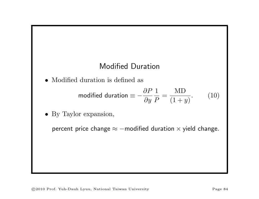
Modified Duration

• Modified duration is defined as

modified duration ≡ −∂P

∂y

1

P=

MD

(1 + y). (10)

• By Taylor expansion,

percent price change ≈ −modified duration× yield change.


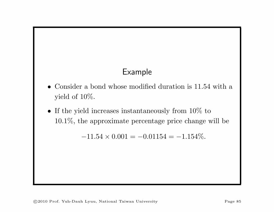
Example

• Consider a bond whose modified duration is 11.54 with a

yield of 10%.

• If the yield increases instantaneously from 10% to

10.1%, the approximate percentage price change will be

−11.54× 0.001 = −0.01154 = −1.154%.


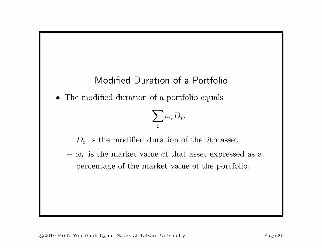
Modified Duration of a Portfolio

• The modified duration of a portfolio equals∑i

ωiDi.

– Di is the modified duration of the ith asset.

– ωi is the market value of that asset expressed as a

percentage of the market value of the portfolio.


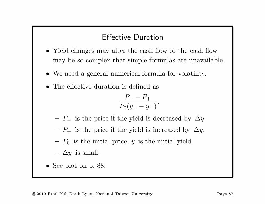
Effective Duration

• Yield changes may alter the cash flow or the cash flow

may be so complex that simple formulas are unavailable.

• We need a general numerical formula for volatility.

• The effective duration is defined as

P− − P+

P0(y+ − y−).

– P− is the price if the yield is decreased by ∆y.

– P+ is the price if the yield is increased by ∆y.

– P0 is the initial price, y is the initial yield.

– ∆y is small.

• See plot on p. 88.


y

P0

P+

P-

y+

y-


Effective Duration (concluded)

• One can compute the effective duration of just about

any financial instrument.

• Duration of a security can be longer than its maturity or

negative!

• Neither makes sense under the maturity interpretation.

• An alternative is to use

P0 − P+

P0 ∆y.

– More economical but less accurate.


The Practices

• Duration is usually expressed in percentage terms—call

it D%—for quick mental calculation.

• The percentage price change expressed in percentage

terms is approximated by

−D% ×∆r

when the yield increases instantaneously by ∆r%.

– Price will drop by 20% if D% = 10 and ∆r = 2

because 10× 2 = 20.

• In fact, D% equals modified duration as originally

defined (prove it!).


Hedging

• Hedging offsets the price fluctuations of the position to

be hedged by the hedging instrument in the opposite

direction, leaving the total wealth unchanged.

• Define dollar duration as

modified duration× price (% of par) = −∂P

∂y.

• The approximate dollar price change per $100 of par

value is

price change ≈ −dollar duration× yield change.


Convexity

• Convexity is defined as

convexity (in periods) ≡ ∂2P

∂y21

P.

• The convexity of a coupon bond is positive (prove it!).

• For a bond with positive convexity, the price rises more

for a rate decline than it falls for a rate increase of equal

magnitude (see plot next page).

• Hence, between two bonds with the same duration, the

one with a higher convexity is more valuable.


0.02 0.04 0.06 0.08Yield

50

100

150

200

250

Price


Convexity (concluded)

• Convexity measured in periods and convexity measured

in years are related by

convexity (in years) =convexity (in periods)

k2

when there are k periods per annum.


Use of Convexity

• The approximation ∆P/P ≈ − duration× yield change

works for small yield changes.

• To improve upon it for larger yield changes, use

∆P

P≈ ∂P

∂y

1

P∆y +

1

2

∂2P

∂y21

P(∆y)2

= −duration×∆y +1

2× convexity× (∆y)2.

• Recall the figure on p. 93.


The Practices

• Convexity is usually expressed in percentage terms—call

it C%—for quick mental calculation.

• The percentage price change expressed in percentage

terms is approximated by −D% ×∆r + C% × (∆r)2/2

when the yield increases instantaneously by ∆r%.

– Price will drop by 17% if D% = 10, C% = 1.5, and

∆r = 2 because

−10× 2 +1

2× 1.5× 22 = −17.

• In fact, C% equals convexity divided by 100 (prove it!).


Effective Convexity

• The effective convexity is defined as

P+ + P− − 2P0

P0 (0.5× (y+ − y−))2 ,

– P− is the price if the yield is decreased by ∆y.

– P+ is the price if the yield is increased by ∆y.

– P0 is the initial price, y is the initial yield.

– ∆y is small.

• Effective convexity is most relevant when a bond’s cash

flow is interest rate sensitive.

• Numerically, choosing the right ∆y is a delicate matter.


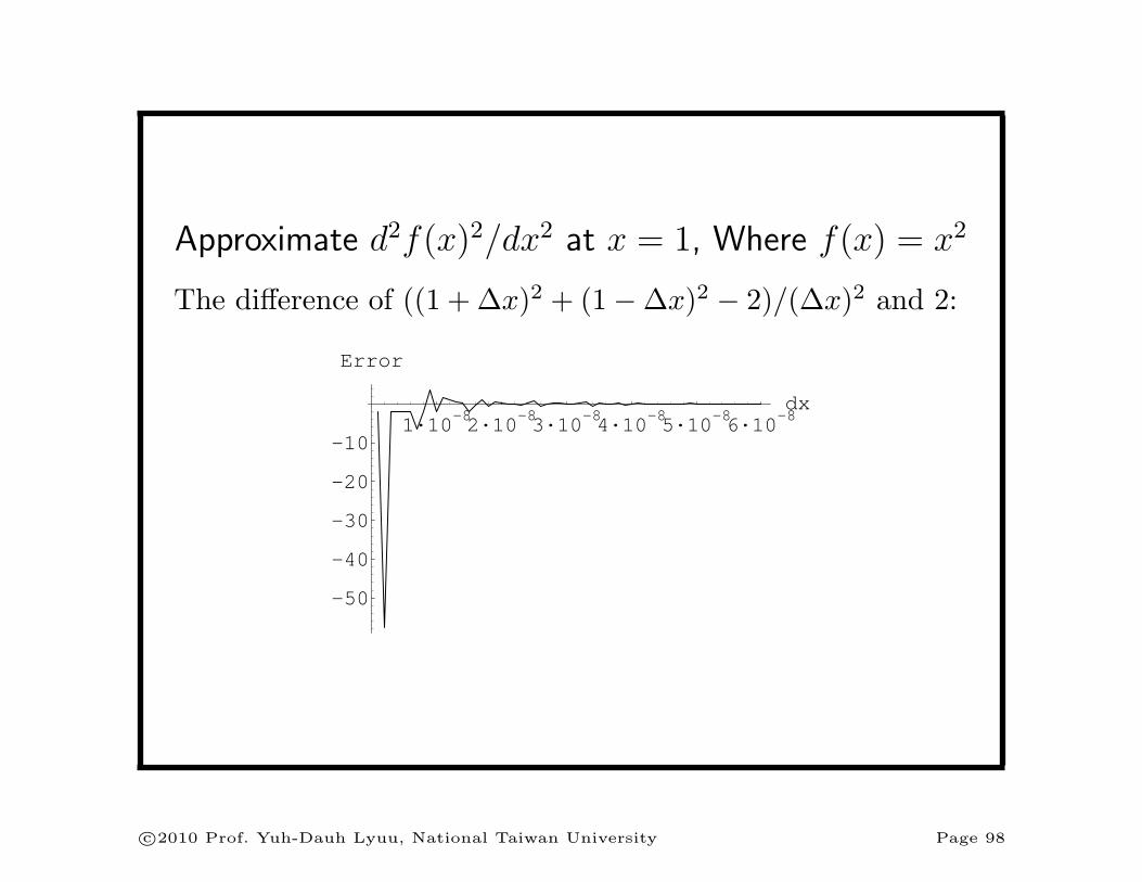
Approximate d2f(x)2/dx2 at x = 1, Where f(x) = x2

The difference of ((1 + ∆x)2 + (1−∆x)2 − 2)/(∆x)2 and 2:

1·10-82·10-83·10-84·10-85·10-86·10-8dx

-50

-40

-30

-20

-10

Error


Term Structure of Interest Rates


Why is it that the interest of money is lower,

when money is plentiful?

— Samuel Johnson (1709–1784)

If you have money, don’t lend it at interest.

Rather, give [it] to someone

from whom you won’t get it back.

— Thomas Gospel 95


Term Structure of Interest Rates

• Concerned with how interest rates change with maturity.

• The set of yields to maturity for bonds forms the term

structure.

– The bonds must be of equal quality.

– They differ solely in their terms to maturity.

• The term structure is fundamental to the valuation of

fixed-income securities.


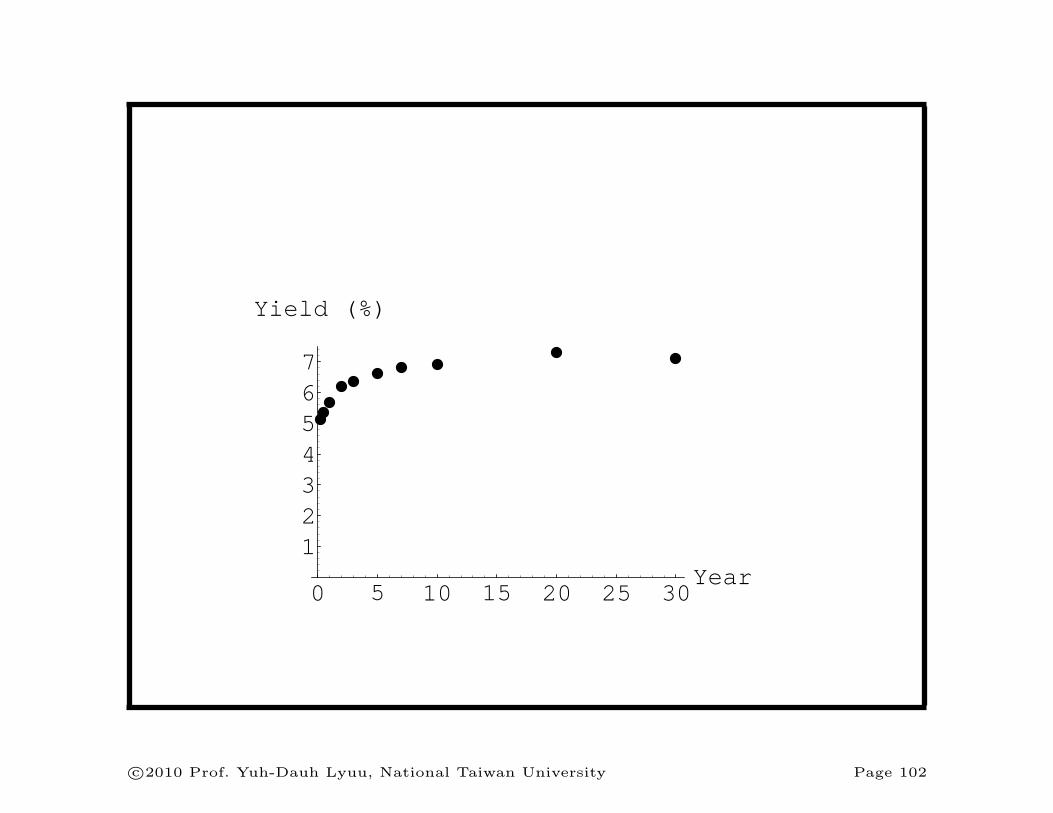
0 5 10 15 20 25 30Year

1234567

Yield (%)


Term Structure of Interest Rates (concluded)

• Term structure often refers exclusively to the yields of

zero-coupon bonds.

• A yield curve plots yields to maturity against maturity.

• A par yield curve is constructed from bonds trading

near par.


Four Typical Shapes

• A normal yield curve is upward sloping.

• An inverted yield curve is downward sloping.

• A flat yield curve is flat.

• A humped yield curve is upward sloping at first but then

turns downward sloping.


Spot Rates

• The i-period spot rate S(i) is the yield to maturity of

an i-period zero-coupon bond.

• The PV of one dollar i periods from now is

[ 1 + S(i) ]−i.

• The one-period spot rate is called the short rate.

• Spot rate curve: Plot of spot rates against maturity.


Problems with the PV Formula

• In the bond price formula,

n∑i=1

C

(1 + y)i+

F

(1 + y)n,

every cash flow is discounted at the same yield y.

• Consider two riskless bonds with different yields to

maturity because of their different cash flow streams:

n1∑i=1

C

(1 + y1)i+

F

(1 + y1)n1,

n2∑i=1

C

(1 + y2)i+

F

(1 + y2)n2.


Problems with the PV Formula (concluded)

• The yield-to-maturity methodology discounts their

contemporaneous cash flows with different rates.

• But shouldn’t they be discounted at the same rate?


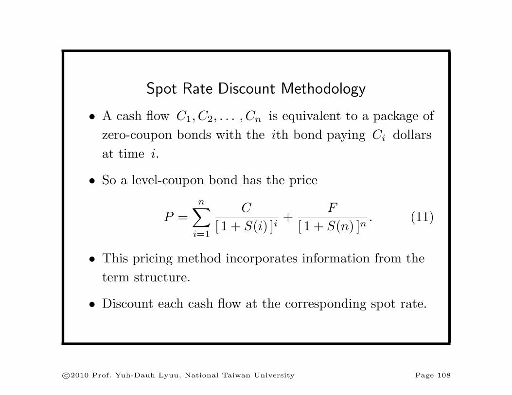
Spot Rate Discount Methodology

• A cash flow C1, C2, . . . , Cn is equivalent to a package of

zero-coupon bonds with the ith bond paying Ci dollars

at time i.

• So a level-coupon bond has the price

P =n∑

i=1

C

[ 1 + S(i) ]i+

F

[ 1 + S(n) ]n. (11)

• This pricing method incorporates information from the

term structure.

• Discount each cash flow at the corresponding spot rate.


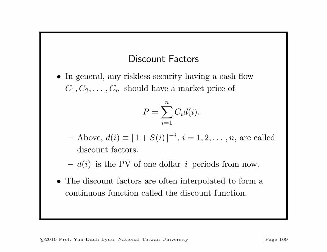
Discount Factors

• In general, any riskless security having a cash flow

C1, C2, . . . , Cn should have a market price of

P =n∑

i=1

Cid(i).

– Above, d(i) ≡ [ 1 + S(i) ]−i, i = 1, 2, . . . , n, are called

discount factors.

– d(i) is the PV of one dollar i periods from now.

• The discount factors are often interpolated to form a

continuous function called the discount function.


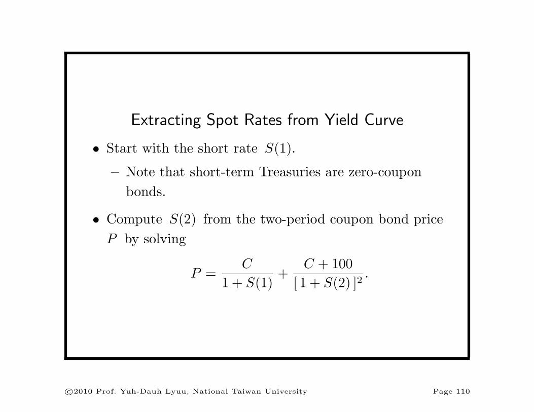
Extracting Spot Rates from Yield Curve

• Start with the short rate S(1).

– Note that short-term Treasuries are zero-coupon

bonds.

• Compute S(2) from the two-period coupon bond price

P by solving

P =C

1 + S(1)+

C + 100

[ 1 + S(2) ]2.


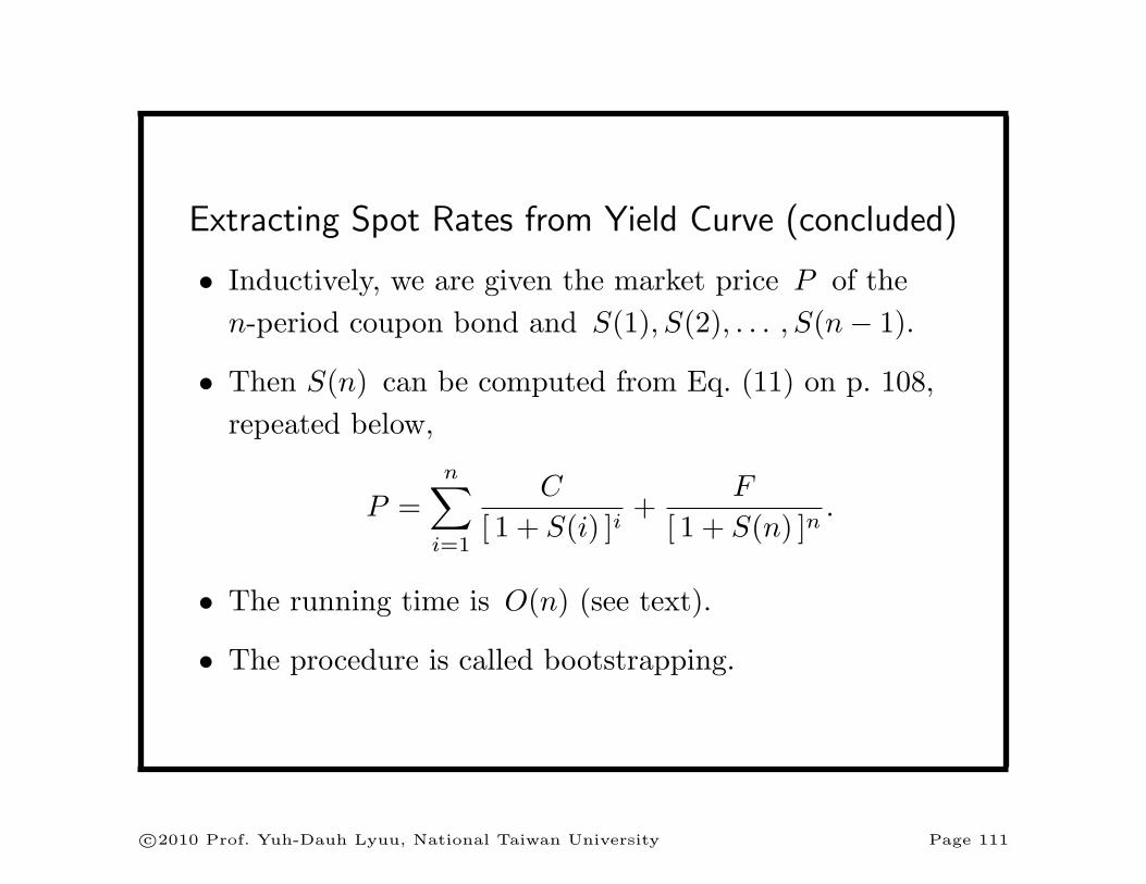
Extracting Spot Rates from Yield Curve (concluded)

• Inductively, we are given the market price P of the

n-period coupon bond and S(1), S(2), . . . , S(n− 1).

• Then S(n) can be computed from Eq. (11) on p. 108,

repeated below,

P =n∑

i=1

C

[ 1 + S(i) ]i+

F

[ 1 + S(n) ]n.

• The running time is O(n) (see text).

• The procedure is called bootstrapping.


Some Problems

• Treasuries of the same maturity might be selling at

different yields (the multiple cash flow problem).

• Some maturities might be missing from the data points

(the incompleteness problem).

• Treasuries might not be of the same quality.

• Interpolation and fitting techniques are needed in

practice to create a smooth spot rate curve.

– Any economic justifications?


Yield Spread

• Consider a risky bond with the cash flow

C1, C2, . . . , Cn and selling for P .

• Were this bond riskless, it would fetch

P ∗ =n∑

t=1

Ct

[ 1 + S(t) ]t.

• Since riskiness must be compensated, P < P ∗.

• Yield spread is the difference between the IRR of the

risky bond and that of a riskless bond with comparable

maturity.


Static Spread

• The static spread is the amount s by which the spot

rate curve has to shift in parallel to price the risky bond:

P =n∑

t=1

Ct

[ 1 + s+ S(t) ]t.

• Unlike the yield spread, the static spread incorporates

information from the term structure.


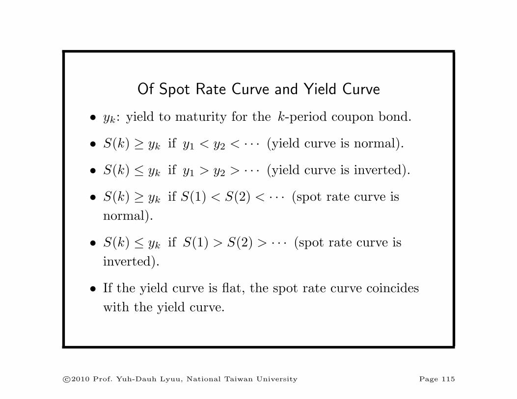
Of Spot Rate Curve and Yield Curve

• yk: yield to maturity for the k-period coupon bond.

• S(k) ≥ yk if y1 < y2 < · · · (yield curve is normal).

• S(k) ≤ yk if y1 > y2 > · · · (yield curve is inverted).

• S(k) ≥ yk if S(1) < S(2) < · · · (spot rate curve is

normal).

• S(k) ≤ yk if S(1) > S(2) > · · · (spot rate curve is

inverted).

• If the yield curve is flat, the spot rate curve coincides

with the yield curve.


Shapes

• The spot rate curve often has the same shape as the

yield curve.

– If the spot rate curve is inverted (normal, resp.), then

the yield curve is inverted (normal, resp.).

• But this is only a trend not a mathematical truth.a

aSee a counterexample in the text.


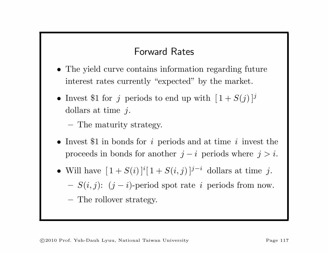
Forward Rates

• The yield curve contains information regarding future

interest rates currently “expected” by the market.

• Invest $1 for j periods to end up with [ 1 + S(j) ]j

dollars at time j.

– The maturity strategy.

• Invest $1 in bonds for i periods and at time i invest the

proceeds in bonds for another j − i periods where j > i.

• Will have [ 1 + S(i) ]i[ 1 + S(i, j) ]j−i dollars at time j.

– S(i, j): (j − i)-period spot rate i periods from now.

– The rollover strategy.


Forward Rates (concluded)

• When S(i, j) equals

f(i, j) ≡[(1 + S(j))j

(1 + S(i))i

]1/(j−i)

− 1, (12)

we will end up with [ 1 + S(j) ]j dollars again.

• By definition, f(0, j) = S(j).

• f(i, j) is called the (implied) forward rates.

– More precisely, the (j − i)-period forward rate i

periods from now.


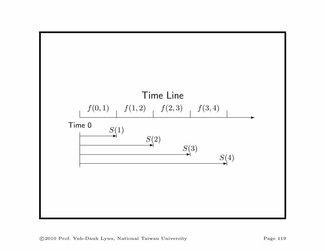
Time Line

-f(0, 1) f(1, 2) f(2, 3) f(3, 4)

Time 0-S(1)

-S(2)

-S(3)

-S(4)


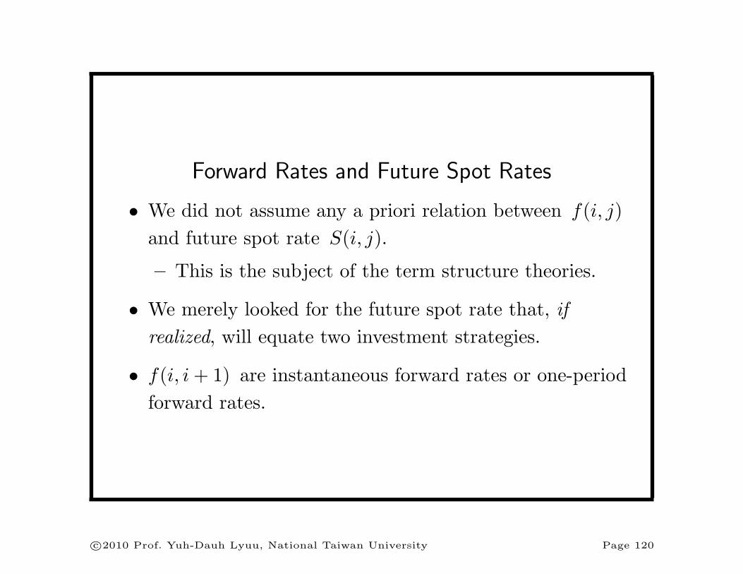
Forward Rates and Future Spot Rates

• We did not assume any a priori relation between f(i, j)

and future spot rate S(i, j).

– This is the subject of the term structure theories.

• We merely looked for the future spot rate that, if

realized, will equate two investment strategies.

• f(i, i+ 1) are instantaneous forward rates or one-period

forward rates.


Spot Rates and Forward Rates

• When the spot rate curve is normal, the forward rate

dominates the spot rates,

f(i, j) > S(j) > · · · > S(i).

• When the spot rate curve is inverted, the forward rate is

dominated by the spot rates,

f(i, j) < S(j) < · · · < S(i).


spot rate curve

forward rate curve

yield curve

(a)

spot rate curve

forward rate curve

yield curve

(b)


Day Count Conventions: Actual/Actual

Documents

Transcript of Day Count Conventions: Actual/Actual