Data Structures - Komputasi · PDF fileJ.E.D.I Author Joyce Avestro Team Joyce Avestro...

J.E.D.I

Data Structures

Version 2.0June 2006

Data Structures 1

J.E.D.I

AuthorJoyce Avestro

TeamJoyce AvestroFlorence BalagtasRommel FeriaReginald HutchersonRebecca OngJohn Paul PetinesSang ShinRaghavan SrinivasMatthew Thompson

Requirements For the Laboratory Exercises

Supported Operating SystemsThe NetBeans IDE 5.5 runs on operating systems that support the Java VM. Below is a list of platforms:

• Microsoft Windows XP Professional SP2 or newer

• Mac OS X 10.4.5 or newer

• Red Hat Fedora Core 3

• Solaris™ 10 Operating System Update 1 (SPARC® and x86/x64 Platform Edition)

NetBeans Enterprise Pack is also known to run on the following platforms: • Microsoft Windows 2000 Professional SP4

• Solaris™ 8 OS (SPARC and x86/x64 Platform Edition) and Solaris 9 OS (SPARC and x86/x64 Platform Edition)

• Various other Linux distributions

Minimum Hardware ConfigurationNote: The NetBeans IDE's minimum screen resolution is 1024x768 pixels.

• Microsoft Windows operating systems:

• Processor: 500 MHz Intel Pentium III workstation or equivalent

• Memory: 512 MB

• Disk space: 850 MB of free disk space

• Linux operating system:

• Processor: 500 MHz Intel Pentium III workstation or equivalent

• Memory: 512 MB


• Solaris OS (SPARC):

• Processor: UltraSPARC II 450 MHz

• Memory: 512 MB


• Solaris OS (x86/x64 Platform Edition):

• Processor: AMD Opteron 100 Series 1.8 GHz

• Memory: 512 MB


• Macintosh OS X operating system:

• Processor: PowerPC G4

• Memory: 512 MB


Recommended Hardware Configuration• Microsoft Windows operating systems:

• Processor: 1.4 GHz Intel Pentium III workstation or equivalent

• Memory: 1 GB

• Disk space: 1 GB of free disk space

• Linux operating system:

• Processor: 1.4 GHz Intel Pentium III or equivalent

• Memory: 1 GB


• Solaris™ OS (SPARC®):

• Processor: UltraSPARC IIIi 1 GHz

• Memory: 1 GB


Data Structures 2

http://www.netbeans.org/community/releases/40/relnotes.html

J.E.D.I

• Solaris™ OS (x86/x64 platform edition):

• Processor: AMD Opteron 100 Series 1.8 GHz

• Memory: 1 GB


• Macintosh OS X operating system:

• Processor: PowerPC G5

• Memory: 1 GB


•• Required Software

NetBeans Enterprise Pack 5.5 Early Access runs on the Java 2 Platform Standard Edition Development Kit 5.0 Update 1 or higher (JDK 5.0, version 1.5.0_01 or higher), which consists of the Java Runtime Environment plus developer tools for compiling, debugging, and running applications written in the Java language. Sun Java System Application Server Platform Edition 9 has been tested with JDK 5.0 update 6.

•• For Solaris, Windows, and Linux, you can download the JDK for

your platform from http://java.sun.com/j2se/1.5.0/download.html

• For Mac OS X, Java 2 Platform Standard Edition (J2SE) 5.0 Release 4, is required. You can download the JDK from Apple's Developer Connection site. Start here: http://developer.apple.com/java (you must register to download the JDK).

Data Structures 3

http://developer.apple.com/java

http://java.sun.com/j2se/1.5.0/download.jsp

J.E.D.I

Table of Contents1 Basic Concepts and Notations............................................................................. 8

1.1 Objectives................................................................................................. 81.2 Introduction.............................................................................................. 81.3 Problem Solving Process ............................................................................. 81.4 Data Type, Abstract Data Type and Data Structure..........................................91.5 Algorithm................................................................................................ 101.6 Addressing Methods.................................................................................. 10

1.6.1 Computed Addressing Method ............................................................. 101.6.2 Link Addressing Method...................................................................... 11

1.6.2.1 Linked Allocation: The Memory Pool............................................... 111.6.2.2 Two Basic Procedures...................................................................12

1.7 Mathematical Functions............................................................................. 131.8 Complexity of Algorithms........................................................................... 14

1.8.1 Algorithm Efficiency........................................................................... 141.8.2 Operations on the O-Notation.............................................................. 151.8.3 Analysis of Algorithms........................................................................ 17

1.9 Summary ............................................................................................... 191.10 Lecture Exercises.................................................................................... 19

2 Stacks........................................................................................................... 212.1 Objectives............................................................................................... 212.2 Introduction............................................................................................. 212.3 Operations.............................................................................................. 222.4 Sequential Representation......................................................................... 232.5 Linked Representation .............................................................................. 242.6 Sample Application: Pattern Recognition Problem..........................................252.7 Advanced Topics on Stacks........................................................................ 30

2.7.1 Multiple Stacks using One-Dimensional Array.........................................302.7.1.1 Three or More Stacks in a Vector S................................................ 302.7.1.2 Three Possible States of a Stack.................................................... 31

2.7.2 Reallocating Memory at Stack Overflow................................................. 312.7.2.1 Memory Reallocation using Garwick's Algorithm............................... 32

2.8 Summary................................................................................................ 362.9 Lecture Exercises...................................................................................... 372.10 Programming Exercises........................................................................... 37

3 Queues.......................................................................................................... 393.1 Objectives............................................................................................... 393.2 Introduction............................................................................................. 393.3 Representation of Queues.......................................................................... 39

3.3.1 Sequential Representation...................................................................403.3.2 Linked Representation........................................................................ 41

3.4 Circular Queue......................................................................................... 423.5 Application: Topological Sorting.................................................................. 44

3.5.1 The Algorithm................................................................................... 453.6 Summary................................................................................................ 473.7 Lecture Exercise....................................................................................... 483.8 Programming Exercises............................................................................. 48

4 Binary Trees .................................................................................................. 494.1 Objectives............................................................................................... 494.2 Introduction............................................................................................. 49

Data Structures 4

J.E.D.I

4.3 Definitions and Related Concepts................................................................ 494.3.1 Properties of a Binary Tree.................................................................. 514.3.2 Types of Binary Tree.......................................................................... 51

4.4 Representation of Binary Trees................................................................... 534.5 Binary Tree Traversals............................................................................... 55

4.5.1 Preorder Traversal............................................................................. 554.5.2 Inorder Traversal............................................................................... 564.5.3 Postorder Traversal............................................................................ 57

4.6 Applications of Binary Tree Traversals......................................................... 594.6.1 Duplicating a Binary Tree.................................................................... 594.6.2 Equivalence of Two Binary Trees ......................................................... 59

4.7 Binary Tree Application: Heaps and the Heapsort Algorithm............................604.7.1 Sift-Up............................................................................................. 614.7.2 Sequential Representation of a Complete Binary Tree..............................614.7.3 The Heapsort Algorithm...................................................................... 63

4.8 Summary................................................................................................ 684.9 Lecture Exercises...................................................................................... 694.10 Programming Exercises........................................................................... 70

5 Trees............................................................................................................. 725.1 Objectives............................................................................................... 725.2 Definitions and Related Concepts................................................................ 72

5.2.1 Ordered Tree .................................................................................... 725.2.2 Oriented Tree ................................................................................... 735.2.3 Free Tree ......................................................................................... 735.2.4 Progression of Trees........................................................................... 74

5.3 Link Representation of Trees...................................................................... 745.4 Forests.................................................................................................... 75

5.4.1 Natural Correspondence: Binary Tree Representation of Forest................. 755.4.2 Forest Traversal ................................................................................ 775.4.3 Sequential Representation of Forests.................................................... 78

5.4.3.1 Preorder Sequential Representation............................................... 795.4.3.2 Family-Order Sequential Representation......................................... 805.4.3.3 Level-Order Sequential Representation........................................... 815.4.3.4 Converting from Sequential to Link Representation.......................... 81

5.5 Arithmetic Tree Representations................................................................. 835.5.1.1 Preorder Sequence with Degrees................................................... 835.5.1.2 Preorder Sequence with Weights................................................... 835.5.1.3 Postorder Sequence with Weights.................................................. 845.5.1.4 Level-Order Sequence with Weights............................................... 84

5.5.2 Application: Trees and the Equivalence Problem..................................... 845.5.2.1 The Equivalence Problem.............................................................. 845.5.2.2 Computer Implementation............................................................ 855.5.2.3 Degeneracy and the Weighting Rule For Union.................................90

5.6 Summary ............................................................................................... 975.7 Lecture Exercises...................................................................................... 975.8 Programming Exercise............................................................................... 98

6 Graphs.......................................................................................................... 996.1 Objectives............................................................................................... 996.2 Introduction............................................................................................. 996.3 Definitions and Related Concepts................................................................ 996.4 Graph Representations............................................................................ 103

6.4.1 Adjacency Matrix for Directed Graphs.................................................. 1036.4.2 Adjacency Lists for Directed Graphs.................................................... 104

Data Structures 5

J.E.D.I

6.4.3 Adjacency Matrix for Undirected Graphs.............................................. 1056.4.4 Adjacency List for Undirected Graphs.................................................. 105

6.5 Graph Traversals.................................................................................... 1066.5.1 Depth First Search........................................................................... 1066.5.2 Breadth First Search ........................................................................ 108

6.6 Minimum Cost Spanning Tree for Undirected Graphs.................................... 1096.6.1.1 MST Theorem............................................................................ 1106.6.1.2 Prim’s Algorithm ....................................................................... 1106.6.1.3 Kruskal's Algorithm ................................................................... 111

6.7 Shortest Path Problems for Directed Graphs................................................1166.7.1 Dijkstra's Algorithm for the SSSP Problem........................................... 1166.7.2 Floyd's Algorithm for the APSP Problem............................................... 119

6.8 Summary.............................................................................................. 1226.9 Lecture Exercises.................................................................................... 1226.10 Programming Exercises.......................................................................... 124

7 Lists............................................................................................................ 1267.1 Objectives............................................................................................. 1267.2 Introduction........................................................................................... 1267.3 Definition and Related Concepts................................................................126

7.3.1 Linear List....................................................................................... 1267.3.2 Generalized List............................................................................... 127

7.4 List Representations................................................................................ 1287.4.1 Sequential Representation of Singly-Linked Linear List ......................... 1287.4.2 Linked Representation of Singly-Linked Linear List .............................. 1297.4.3 Singly-Linked Circular List ................................................................ 1297.4.4 Singly-Linked List with Header Nodes.................................................. 1337.4.5 Doubly-Linked List ........................................................................... 133

7.5 Application: Polynomial Arithmetic............................................................ 1357.5.1 Polynomial Arithmetic Algorithms....................................................... 137

7.5.1.1 Polynomial Addition .................................................................. 1387.5.1.2 Polynomial Subtraction............................................................... 1417.5.1.3 Polynomial Multiplication............................................................ 142

7.6 Dynamic Memory Allocation..................................................................... 1437.6.1 Managing the Memory Pool................................................................ 1437.6.2 Sequential-Fit Methods: Reservation................................................... 1447.6.3 Sequential-Fit Methods: Liberation..................................................... 146

7.6.3.1 Sorted-List Technique ............................................................... 1477.6.3.2 Boundary-Tag Technique ........................................................... 150

7.6.4 Buddy-System Methods.................................................................... 1527.6.4.1 Binary Buddy-System Method .....................................................1527.6.4.2 Reservation.............................................................................. 152

7.6.5 External and Internal Fragmentation in DMA........................................ 1597.7 Summary.............................................................................................. 1597.8 Lecture Exercises.................................................................................... 1607.9 Programming Exercises........................................................................... 161

8 Tables......................................................................................................... 1628.1 Objectives............................................................................................. 1628.2 Introduction........................................................................................... 1628.3 Definitions and Related Concepts.............................................................. 162

8.3.1 Types of Keys ................................................................................. 1638.3.2 Operations...................................................................................... 1638.3.3 Implementation............................................................................... 163

8.3.3.1 Implementation Factors.............................................................. 163

Data Structures 6

J.E.D.I

8.3.3.2 Advantages.............................................................................. 1648.4 Tables and Searching.............................................................................. 164

8.4.1 Table Organization........................................................................... 1648.4.2 Sequential Search in an Unordered Table ............................................1648.4.3 Searching in an Ordered Table .......................................................... 165

8.4.3.1 Indexed Sequential Search ........................................................ 1658.4.3.2 Binary Search .......................................................................... 1668.4.3.3 Multiplicative Binary Search ....................................................... 1678.4.3.4 Fibonacci Search ...................................................................... 167

8.5 Summary.............................................................................................. 1708.6 Lecture Exercises.................................................................................... 1708.7 Programming Exercise............................................................................. 170

9 Binary Search Trees....................................................................................... 1719.1 Objectives............................................................................................. 1719.2 Introduction........................................................................................... 1719.3 Operations on Binary Search Trees............................................................ 171

9.3.1 Searching ...................................................................................... 1739.3.2 Insertion ........................................................................................ 1739.3.3 Deletion ......................................................................................... 1749.3.4 Time Complexity of BST.................................................................... 179

9.4 Balanced Binary Search Trees................................................................... 1799.4.1 AVL Tree ........................................................................................ 179

9.4.1.1 Tree Balancing.......................................................................... 1809.5 Summary.............................................................................................. 1849.6 Lecture Exercise..................................................................................... 1859.7 Programming Exercise............................................................................. 185

10 Hash Table and Hashing Techniques............................................................... 18610.1 Objectives............................................................................................ 18610.2 Introduction......................................................................................... 18610.3 Simple Hash Techniques........................................................................ 187

10.3.1 Prime Number Division Method ........................................................ 18710.3.2 Folding......................................................................................... 187

10.4 Collision Resolution Techniques .............................................................. 18910.4.1 Chaining....................................................................................... 18910.4.2 Use of Buckets............................................................................... 19010.4.3 Open Addressing (Probing).............................................................. 191

10.4.3.1 Linear Probing......................................................................... 19110.4.3.2 Double Hashing....................................................................... 192

10.5 Dynamic Files & Hashing........................................................................ 19510.5.1 Extendible Hashing......................................................................... 195

10.5.1.1 Trie....................................................................................... 19510.5.2 Dynamic Hashing........................................................................... 197

10.6 Summary............................................................................................. 19810.7 Lecture Exercises.................................................................................. 19910.8 Programming Exercises.................................................................................................................. 199

Appendix A: Bibliography................................................................................... 200Appendix B: Answers to Selected Exercises........................................................... 201

Chapter 1.................................................................................................... 201Chapter 2 .................................................................................................... 201Chapter 3 .................................................................................................... 202Chapter 4 .................................................................................................... 202Chapter 5 .................................................................................................... 203

Data Structures 7

J.E.D.I

Chapter 6 .................................................................................................... 205Chapter 7 .................................................................................................... 206Chapter 8 .................................................................................................... 207Chapter 9 .................................................................................................... 208Chapter 10 .................................................................................................. 209

Data Structures 8

J.E.D.I

1 Basic Concepts and Notations

1.1 Objectives

At the end of the lesson, the student should be able to:

• Explain the process of problem solving

• Define data type, abstract data type and data structure

• Identify the properties of an algorithm

• Differentiate the two addressing methods - computed addressing and link addressing

• Use the basic mathematical functions to analyze algorithms

• Measure complexity of algorithms by expressing the efficiency in terms of time complexity and big-O notation

1.2 Introduction

In creating a solution in the problem solving process, there is a need for representing higher level data from basic information and structures available at the machine level. There is also a need for synthesis of the algorithms from basic operations available at the machine level to manipulate higher-level representations. These two play an important role in obtaining the desired result. Data structures are needed for data representation while algorithms are needed to operate on data to produce correct output.

In this lesson we will discuss the basic concepts behind the problem-solving process, data types, abstract data types, algorithm and its properties, the addressing methods, useful mathematical functions and complexity of algorithms.

1.3 Problem Solving Process

Programming is a problem-solving process, i.e., the problem is identified, the data to manipulate and work on is distinguished and the expected result is determined. It is implemented in a machine known as a computer and the operations provided by the machine is used to solve the given problem. The problem solving process could be viewed in terms of domains – problem, machine and solution.

Problem domain includes the input or the raw data to process, and the output or the processed data. For instance, in sorting a set of numbers, the raw data is set of numbers in the original order and the processed data is the sorted numbers.

The machine domain consists of storage medium and processing unit. The storage

Data Structures 9

J.E.D.I

medium – bits, bytes, words, etc – consists of serially arranged bits that are addressable as a unit. The processing units allow us to perform basic operations that include arithmetic, comparison and so on.

Solution domain, on the other hand, links the problem and machine domains. It is at the solution domain where structuring of higher level data structures and synthesis of algorithms are of concern.

1.4 Data Type, Abstract Data Type and Data Structure

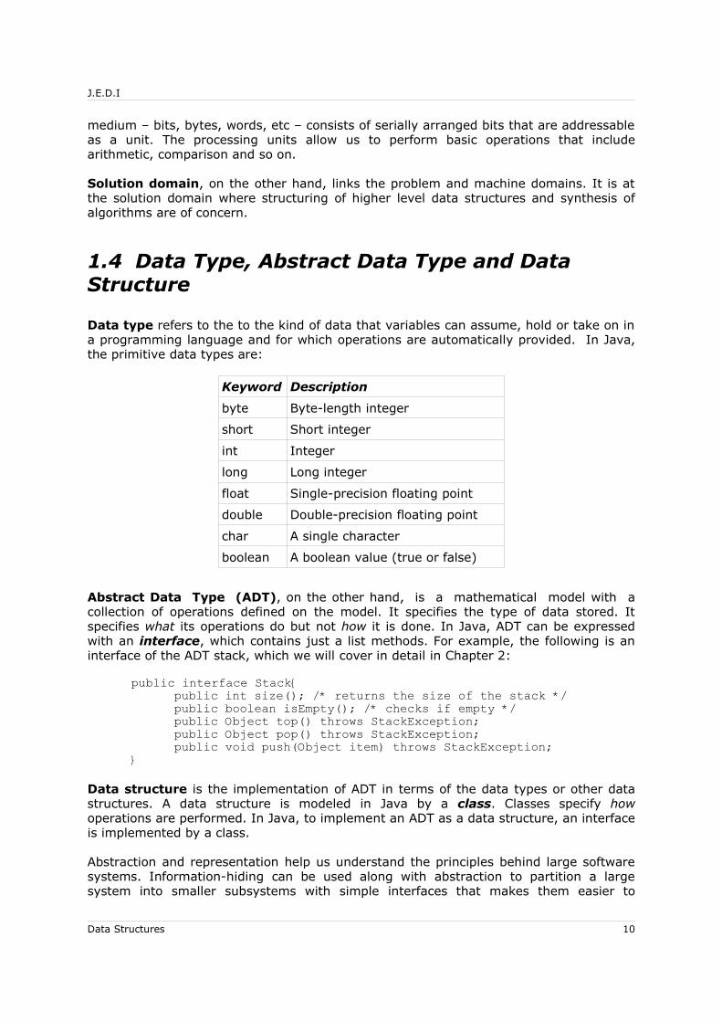
Data type refers to the to the kind of data that variables can assume, hold or take on in a programming language and for which operations are automatically provided. In Java, the primitive data types are:

Keyword Description

byte Byte-length integer

short Short integer

int Integer

long Long integer

float Single-precision floating point

double Double-precision floating point

char A single character

boolean A boolean value (true or false)

Abstract Data Type (ADT), on the other hand, is a mathematical model with a collection of operations defined on the model. It specifies the type of data stored. It specifies what its operations do but not how it is done. In Java, ADT can be expressed with an interface, which contains just a list methods. For example, the following is an interface of the ADT stack, which we will cover in detail in Chapter 2:

public interface Stack{public int size(); /* returns the size of the stack */public boolean isEmpty(); /* checks if empty */public Object top() throws StackException;public Object pop() throws StackException;public void push(Object item) throws StackException;

}

Data structure is the implementation of ADT in terms of the data types or other data structures. A data structure is modeled in Java by a class. Classes specify how operations are performed. In Java, to implement an ADT as a data structure, an interface is implemented by a class.

Abstraction and representation help us understand the principles behind large software systems. Information-hiding can be used along with abstraction to partition a large system into smaller subsystems with simple interfaces that makes them easier to

Data Structures 10

J.E.D.I

understand and use.

1.5 Algorithm

Algorithm is a finite set of instructions which, if followed, will accomplish a task. It has five important properties: finiteness, definiteness, input, output and effectiveness. Finiteness means an algorithm must terminate after a finite number of steps. Definiteness is ensured if every step of an algorithm is precisely defined. For example, "divide by a number x" is not sufficient. The number x must be define precisely, say a positive integer. Input is the domain of the algorithm which could be zero or more quantities. Output is the set of one or more resulting quantities which is also called the range of the algorithm. Effectiveness is ensured if all the operations in the algorithm are sufficiently basic that they can, in principle, be done exactly and in finite time by a person using paper and pen.

Consider the following example:

public class Minimum {

public static void main(String[] args) {int a[] = { 23, 45, 71, 12, 87, 66, 20, 33, 15, 69 };int min = a[0]; for (int i = 1; i < a.length; i++) {

if (a[i] < min) min = a[i];}System.out.println("The minimum value is: " + min);

}}

The Java code above returns the minimum value from an array of integers. There is no user input since the data from where to get the minimum is already in the program. That is, for the input and output properties. Each step in the program is precisely defined. Hence, it is definite. The declaration, the for loop and the statement to output will all take a finite time to execute. Thus, the finiteness property is satisfied. And when run, it returns the minimum among the values in the array so it is said to be effective.

All the properties of an algorithm must be ensured in writing an algorithm.

1.6 Addressing Methods

In creating a data structure, it is important to determine how to access the data items. It is determined by the addressing method used. There are two types of addressing methods in general – computed and link addressing methods.

1.6.1 Computed Addressing Method

Computed addressing method is used to access the elements of a structure in pre-allocated space. It is essentially static, an array for example:

Data Structures 11

J.E.D.I

int x[] = new int[10];

A data item can be accessed directly by knowing the index on where it is stored.

1.6.2 Link Addressing Method

This addressing method provides the mechanism for manipulating dynamic structures where the size and shape are not known beforehand or if the size and shape changes at runtime. Central to this method is the concept of a node containing at least two fields: INFO and LINK.

Figure 1.1 Node Structure

In Java,

class Node{Object info;Node link;Node(){}Node(Object o, Node l){

info = o;link = l;

}}

1.6.2.1 Linked Allocation: The Memory Pool

The memory pool is the source of the nodes from which linked structures are built. It is also known as the list of available space (or nodes) or simply the avail list:

Figure 1.2 Avail List

Data Structures 12

J.E.D.I

The following is the Java class for AvailList:

class AvailList {Node head;AvailList(){

head = null;}AvailList(Node n){

head = n;}

}

Creating the avail list is as simple as declaring:

AvailList avail = new AvailList();

1.6.2.2 Two Basic Procedures

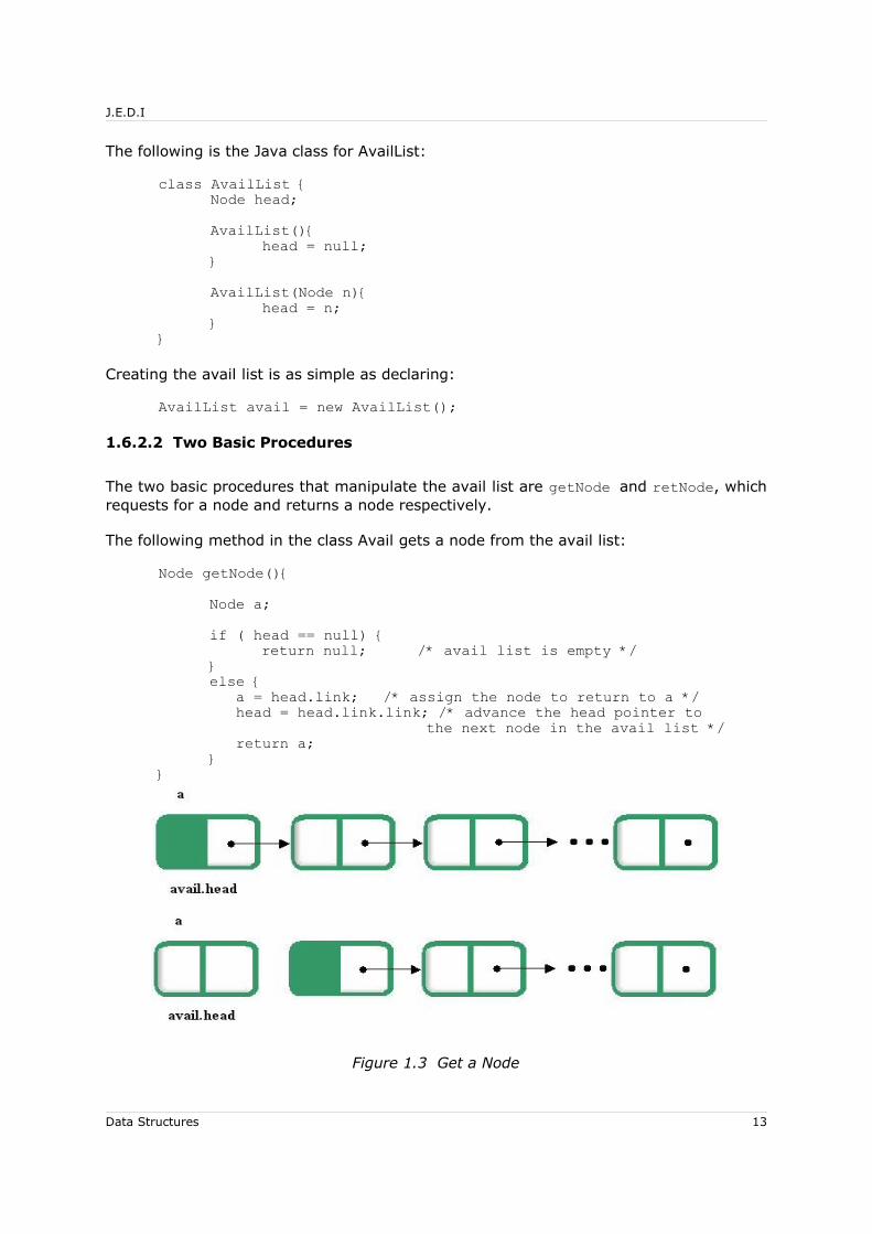
The two basic procedures that manipulate the avail list are getNode and retNode, which requests for a node and returns a node respectively.

The following method in the class Avail gets a node from the avail list:

Node getNode(){Node a;if ( head == null) {

return null; /* avail list is empty */}else {

a = head.link; /* assign the node to return to a */ head = head.link.link; /* advance the head pointer to

the next node in the avail list */ return a;}

}

Figure 1.3 Get a Node

Data Structures 13

J.E.D.I

while the following method in the class Avail returns a node to the avail list:

void retNode(Node n){n.link = head.link; /* adds the new node at the start

of the avail list */head.link = n;

}

Figure 1.4 Return a Node

Figure 1.5

The two methods could be used by data structures that use link allocation in getting nodes from, and returning nodes to the memory pool.

1.7 Mathematical Functions

Mathematical functions are useful in the creation and analysis of algorithms. In this section, some of the most basic and most commonly used functions with their properties are listed.

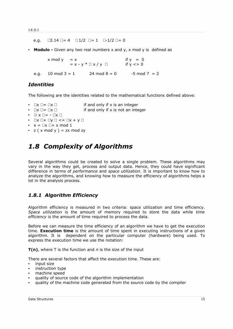
• Floor of x - the greatest integer less than or equal to x, where x is any real number.

Notation: x

e.g. 3.14 = 3 1/2 = 0 -1/2 = - 1

• Ceiling of x - is the smallest integer greater than or equal to x, where x is any real number.

Notation : x

Data Structures 14

J.E.D.I

e.g. 3.14 = 4 1/2 = 1 -1/2 = 0

• Modulo - Given any two real numbers x and y, x mod y is defined as

x mod y = x if y = 0 = x - y * x / y if y <> 0

e.g. 10 mod 3 = 1 24 mod 8 = 0 -5 mod 7 = 2

Identities

The following are the identities related to the mathematical functions defined above:

• x = x if and only if x is an integer• x = x if and only if x is not an integer• - x = - x • x + y <= x + y • x = x + x mod 1• z ( x mod y ) = zx mod zy

1.8 Complexity of Algorithms

Several algorithms could be created to solve a single problem. These algorithms may vary in the way they get, process and output data. Hence, they could have significant difference in terms of performance and space utilization. It is important to know how to analyze the algorithms, and knowing how to measure the efficiency of algorithms helps a lot in the analysis process.

1.8.1 Algorithm Efficiency

Algorithm efficiency is measured in two criteria: space utilization and time efficiency. Space utilization is the amount of memory required to store the data while time efficiency is the amount of time required to process the data.

Before we can measure the time efficiency of an algorithm we have to get the execution time. Execution time is the amount of time spent in executing instructions of a given algorithm. It is dependent on the particular computer (hardware) being used. To express the execution time we use the notation:

T(n), where T is the function and n is the size of the input

There are several factors that affect the execution time. These are: • input size• instruction type • machine speed• quality of source code of the algorithm implementation • quality of the machine code generated from the source code by the compiler

Data Structures 15

J.E.D.I

The Big-Oh Notation

Although T(n) gives the actual amount of time in the execution of an algorithm, it is easier to classify complexities of algorithm using a more general notation, the Big-Oh (or simply O) notation. T(n) grows at a rate proportional to n and thus T(n) is said to have “order of magnitude n” denoted by the O-notation:

T(n) = O(n)

This notation is used to describe the time or space complexity of an algorithm. It gives an approximate measure of the computing time of an algorithm for large number of input. Formally, O-notation is defined as:

g(n) = O(f(n)) if there exists two constants c and n0 such that | g(n) | <= c * | f(n) | for all n >= n0.

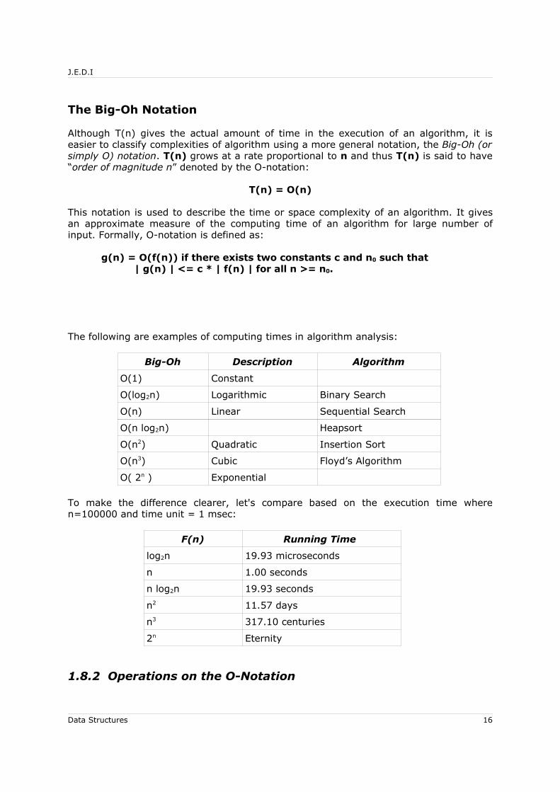
The following are examples of computing times in algorithm analysis:

Big-Oh Description Algorithm

O(1) Constant

O(log2n) Logarithmic Binary Search

O(n) Linear Sequential Search

O(n log2n) Heapsort

O(n2) Quadratic Insertion Sort

O(n3) Cubic Floyd’s Algorithm

O( 2n ) Exponential

To make the difference clearer, let's compare based on the execution time where n=100000 and time unit = 1 msec:

F(n) Running Time

log2n 19.93 microseconds

n 1.00 seconds

n log2n 19.93 seconds

n2 11.57 days

n3 317.10 centuries

2n Eternity

1.8.2 Operations on the O-Notation

Data Structures 16

J.E.D.I

• Rule for Sums

Suppose that T1(n) = O( f(n) ) and T2(n) = O( g(n) ). Then, t(n) = T1(n) + T2(n) = O( max( f(n), g(n) ) ).

Proof : By definition of the O-notation, T1(n) ≤ c1 f(n) for n ≥ n1 and T2(n) ≤ c2 g(n) for n ≥ n2.

Let n0 = max(n2, n2). ThenT1(n) + T2(n) ≤ c1 f(n) + c2 g(n) n ≥ n0.

≤ (c1 + c2) max(f(n),g(n)) n ≥ n0.≤ c max ( f(n), g(n) ) n ≥ n0.

Thus, T(n) = T1(n) + T2(n) = O( max( f(n), g(n) ) ).

For example, 1. T(n) = 3n3 + 5n2 = O(n3)2. T(n) = 2n + n4 + nlog2n = O(2n)

• Rule for Products

Suppose that T1(n) = O( f(n) ) and T2(n) = O( g(n) ). Then, T(n) = T1(n) * T2(n) = O( f(n) * g(n) ).

For example, consider the algorithm below:

for(int i=1; i<n-1; i++){for(int i=1; i<=n; i++){

steps taking O(1) time }

}

Since the steps in the inner loop will take n + n-1 + n-2 + ... + 2 + 1 times,

then n(n+1)/2 = n2/2 + n/2= O(n2)

Example: Consider the code snippet below:

for (i=1; i <= n, i++)for (j=1; j <= n, j++)

// steps which take O(1) time

Since the steps in the inner loop will take n + n-1 + n-2 + ... + 2 + 1 times, then the running time is

n( n+1 ) / 2 = n2 / 2 + n / 2

= O( n2 )

Data Structures 17

J.E.D.I

1.8.3 Analysis of Algorithms

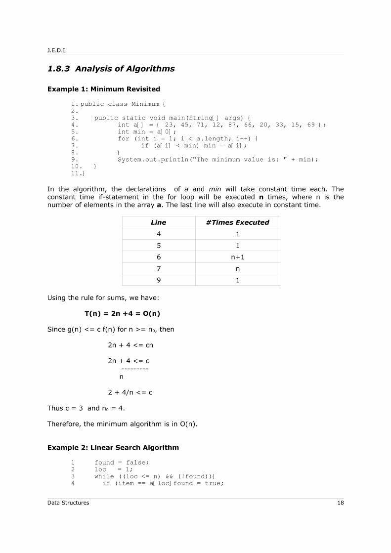
Example 1: Minimum Revisited

1. public class Minimum {2.3. public static void main(String[] args) {4. int a[] = { 23, 45, 71, 12, 87, 66, 20, 33, 15, 69 };5. int min = a[0]; 6. for (int i = 1; i < a.length; i++) {7. if (a[i] < min) min = a[i];8. }9. System.out.println("The minimum value is: " + min);10. }11.}

In the algorithm, the declarations of a and min will take constant time each. The constant time if-statement in the for loop will be executed n times, where n is the number of elements in the array a. The last line will also execute in constant time.

Line #Times Executed

4 1

5 1

6 n+1

7 n

9 1

Using the rule for sums, we have:

T(n) = 2n +4 = O(n)

Since g(n) <= c f(n) for n >= n0, then

2n + 4 <= cn

2n + 4 <= c ---------

n

2 + 4/n <= c

Thus c = 3 and n0 = 4.

Therefore, the minimum algorithm is in O(n).

Example 2: Linear Search Algorithm

1 found = false;2 loc = 1;3 while ((loc <= n) && (!found)){4 if (item == a[loc]found = true;

Data Structures 18

J.E.D.I

5 else loc = loc + 1;6 }

STATEMENT # of times executed

1 1

2 1

3 n + 1

4 n

5 n

T( n ) = 3n + 3 so that T( n ) = O( n )

Since g( n ) <= c f( n ) for n >= n 0, then

3n + 3 <= c n

(3n + 3)/n <= c = 3 + 3 / n <= c

Thus c = 4 and n0 = 3.

The following are the general rules on determining the running time of an algorithm:

● FOR loops

➔ At most the running time of the statement inside the for loop times the number of iterations.

● NESTED FOR loops

➔ Analysis is done from the inner loop going outward. The total running time of a statement inside a group of for loops is the running time of the statement multiplied by the product of thesizes of all the for loops.

● CONSECUTIVE STATEMENTS

➔ The statement with the maximum running time.

● IF/ELSE

➔ Never more than the running time of the test plus the larger of the running times of the conditional block of statements.

Data Structures 19

J.E.D.I

1.9 Summary • Programming as a problem solving process could be viewed in terms of 3 domains

– problem, machine and solution.

• Data structures provide a way for data representation. It is an implementation of ADT.

• An algorithm is a finite set of instructions which, if followed, will accomplish a task. It has five important properties: finiteness, definiteness, input, output and effectiveness.

• Addressing methods define how the data items are accessed. Two general types are computed and link addressing.

• Algorithm efficiency is measured in two criteria: space utilization and time efficiency. The O-notation gives an approximate measure of the computing time of an algorithm for large number of input

1.10 Lecture Exercises

1. Floor, Ceiling and Modulo Functions. Compute for the resulting value:

a) -5.3 b) 6.14 c) 8 mod 7d) 3 mod –4e) –5 mod 2f) 10 mod 11 g) (15 mod –9) + 4.3

2. What is the time complexity of the algorithm with the following running times?

a) 3n5 + 2n3 + 3n +1b) n3/2+n2/5+n+1c) n5+n2+nd) n3 + lg n + 34

3. Suppose we have two parts in an algorithm, the first part takes T(n1)=n3+n+1 time to execute and the second part takes T(n2) = n5+n2+n, what is the time complexity of the algorithm if part 1 and part 2 are executed one at a time?

4. Sort the following time complexities in ascending order.

0(n log2 n) 0(n2) 0(n) 0(log2 n) 0(n2 log2 n)

0(1) 0(n3) 0(nn) 0(2n) 0(log2 log2 n)

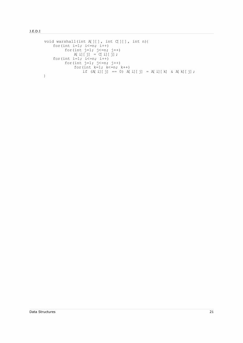
5. What is the execution time and time complexity of the algorithm below?

Data Structures 20

J.E.D.I

void warshall(int A[][], int C[][], int n){for(int i=1; i<=n; i++)

for(int j=1; j<=n; j++)A[i][j] = C[i][j];

for(int i=1; i<=n; i++)for(int j=1; j<=n; j++)

for(int k=1; k<=n; k++)if (A[i][j] == 0) A[i][j] = A[i][k] & A[k][j];

}

Data Structures 21

J.E.D.I

2 Stacks

2.1 Objectives


• Explain the basic concepts and operations on the ADT stack

• Implement the ADT stack using sequential and linked representation

• Discuss applications of stack: the pattern recognition problem and conversion from infix to postfix

• Explain how multiple stacks can be stored using one-dimensional array

• Reallocate memory during stack overflow in multiple-stack array using unit-shift policy and Garwick's algorithm

2.2 Introduction

Stack is a linearly ordered set of elements having the the discipline of last-in, first out, hence it is also known as LIFO list. It is similar to a stack of boxes in a warehouse, where only the top box could be retrieved and there is no access to the other boxes. Also, adding a box means putting it at the top of the stack.

Stacks are used in pattern recognition, lists and tree traversals, evaluation of expressions, resolving recursions and a lot more. The two basic operations for data manipulation are push and pop, which are insertion into and deletion from the top of stack respectively.

Just like what was mentioned in Chapter 1, interface (Application Program Interface or API) is used to implement ADT in Java. The following is the Java interface for stack:

public interface Stack{public int size(); /* returns the size of the stack */public boolean isEmpty(); /* checks if empty */public Object top() throws StackException;public Object pop() throws StackException;public void push(Object item) throws StackException;

}

StackException is an extension of RuntimeException:

class StackException extends RuntimeException{public StackException(String err){

super(err);}

}

Stacks has two possible implementations – a sequentially allocated one-dimensional

Data Structures 22

J.E.D.I

array (vector) or a linked linear list. However, regardless of implementation, the interface Stack will be used.

2.3 Operations

The following are the operations on a stack:• Getting the size• Checking if empty• Getting the top element without deleting it from the stack• Insertion of new element onto the stack (push)• Deletion of the top element from the stack (pop)

Figure 1.6 PUSH Operation

Figure 1.7

Figure 1.8 POP Operation

Data Structures 23

J.E.D.I

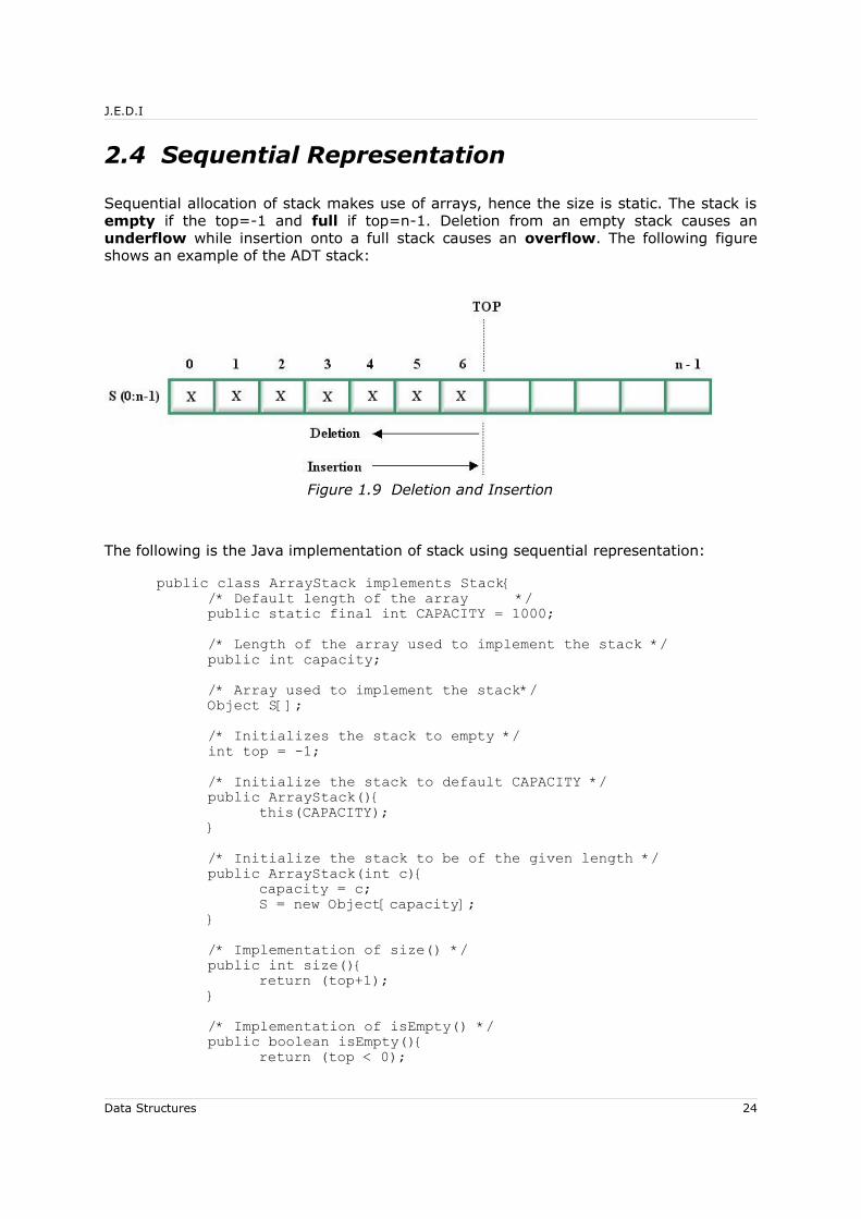
2.4 Sequential Representation

Sequential allocation of stack makes use of arrays, hence the size is static. The stack is empty if the top=-1 and full if top=n-1. Deletion from an empty stack causes an underflow while insertion onto a full stack causes an overflow. The following figure shows an example of the ADT stack:

Figure 1.9 Deletion and Insertion

The following is the Java implementation of stack using sequential representation:

public class ArrayStack implements Stack{/* Default length of the array */public static final int CAPACITY = 1000;/* Length of the array used to implement the stack */public int capacity;/* Array used to implement the stack*/Object S[];/* Initializes the stack to empty */int top = -1;/* Initialize the stack to default CAPACITY */public ArrayStack(){

this(CAPACITY);}/* Initialize the stack to be of the given length */public ArrayStack(int c){

capacity = c;S = new Object[capacity];

}/* Implementation of size() */public int size(){

return (top+1);}/* Implementation of isEmpty() */public boolean isEmpty(){

return (top < 0);

Data Structures 24

J.E.D.I

}/* Implementation of top() */public Object top(){

if (isEmpty()) throw newStackException("Stack empty.");

return S[top];}/* Implementation of pop() */public Object pop(){

Object item;if (isEmpty())

throw new StackException("Stack underflow.");item = S[top];S[top--] = null;return item;

}/* Implementation of push() */public void push(Object item){

if (size()==capacity)throw new StackException("Stack overflow.");

S[++top]=item;}

}

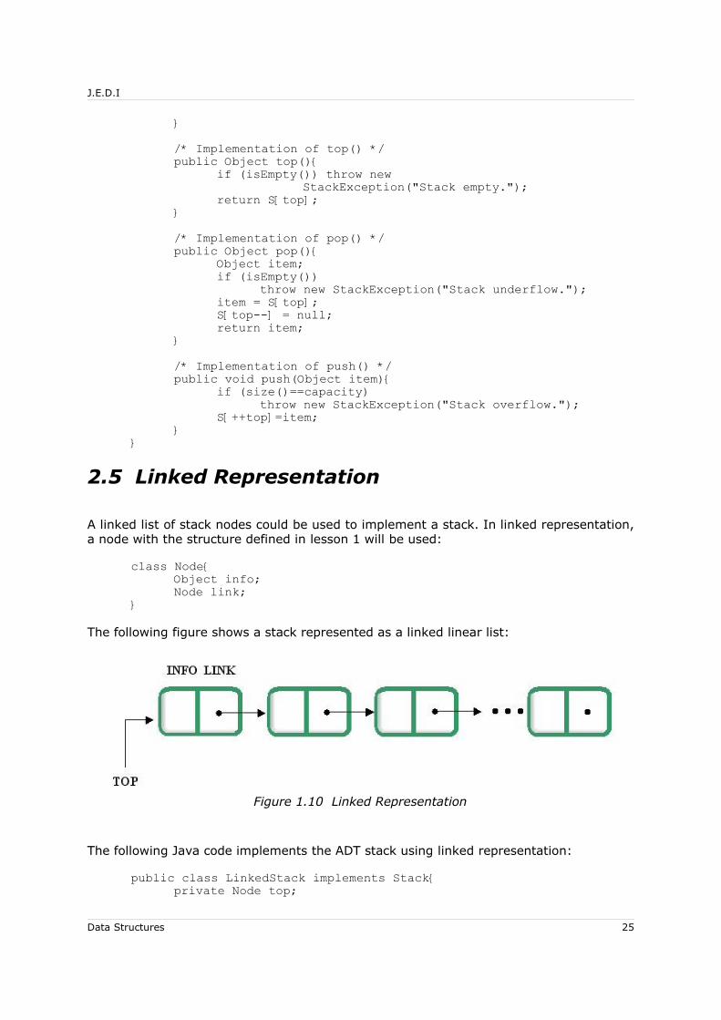
2.5 Linked Representation

A linked list of stack nodes could be used to implement a stack. In linked representation, a node with the structure defined in lesson 1 will be used:

class Node{Object info;Node link;

}

The following figure shows a stack represented as a linked linear list:

Figure 1.10 Linked Representation

The following Java code implements the ADT stack using linked representation:

public class LinkedStack implements Stack{private Node top;

Data Structures 25

J.E.D.I

/* The number of elements in the stack */private int numElements = 0;/* Implementation of size() */public int size(){

return (numElements);}/* Implementation of isEmpty() */public boolean isEmpty(){

return (top == null);}/* Implementation of top() */public Object top(){

if (isEmpty()) throw new StackException("Stack empty.");

return top.info;}/* Implementation of pop() */public Object pop(){

Node temp;if (isEmpty())

throw new StackException("Stack underflow.");temp = top;top = top.link;return temp.info;

}/* Implementation of push() */public void push(Object item){

Node newNode = new Node();newNode.info = item;newNode.link = top;top = newNode;

}}

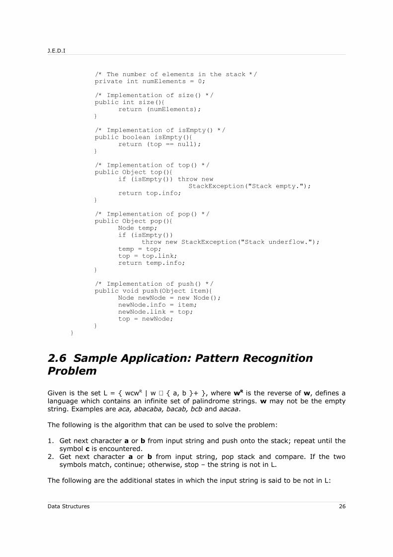
2.6 Sample Application: Pattern Recognition Problem

Given is the set L = { wcwR | w ⊂ { a, b }+ }, where wR is the reverse of w, defines a language which contains an infinite set of palindrome strings. w may not be the empty string. Examples are aca, abacaba, bacab, bcb and aacaa.

The following is the algorithm that can be used to solve the problem:

1. Get next character a or b from input string and push onto the stack; repeat until the symbol c is encountered.

2. Get next character a or b from input string, pop stack and compare. If the two symbols match, continue; otherwise, stop – the string is not in L.

The following are the additional states in which the input string is said to be not in L:

Data Structures 26

J.E.D.I

1. The end of the string is reached but no c is encountered.2. The end of the string is reached but the stack is not empty.3. The stack is empty but the end of the string is not yet reached.

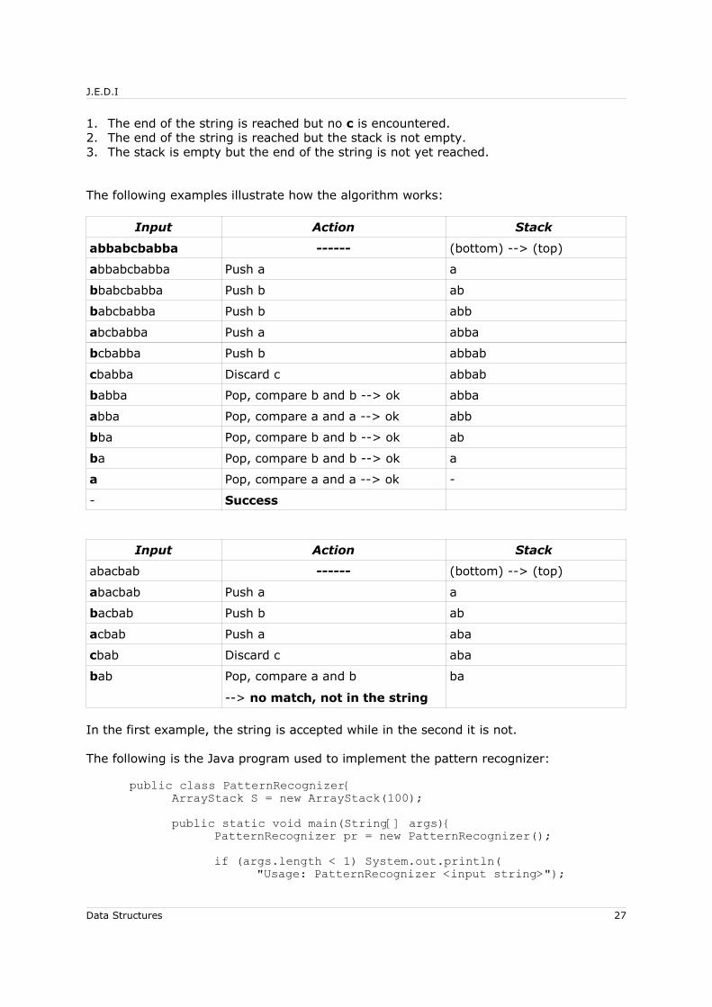
The following examples illustrate how the algorithm works:

Input Action Stack

abbabcbabba ------ (bottom) --> (top)

abbabcbabba Push a a

bbabcbabba Push b ab

babcbabba Push b abb

abcbabba Push a abba

bcbabba Push b abbab

cbabba Discard c abbab

babba Pop, compare b and b --> ok abba

abba Pop, compare a and a --> ok abb

bba Pop, compare b and b --> ok ab

ba Pop, compare b and b --> ok a

a Pop, compare a and a --> ok -

- Success

Input Action Stack

abacbab ------ (bottom) --> (top)

abacbab Push a a

bacbab Push b ab

acbab Push a aba

cbab Discard c aba

bab Pop, compare a and b

--> no match, not in the string

ba

In the first example, the string is accepted while in the second it is not.

The following is the Java program used to implement the pattern recognizer:

public class PatternRecognizer{ArrayStack S = new ArrayStack(100);public static void main(String[] args){

PatternRecognizer pr = new PatternRecognizer();if (args.length < 1) System.out.println(

"Usage: PatternRecognizer <input string>");

Data Structures 27

J.E.D.I

else {boolean inL = pr.recognize(args[0]);if (inL) System.out.println(args[0] +

" is in the language.");else System.out.println(args[0] +

" is not in the language.");}

}boolean recognize(String input){

int i=0; /* Current character indicator *//* While c is not encountered, push the character

onto the stack */while ((i < input.length()) &&

(input.charAt(i) != 'c')){S.push(input.substring(i, i+1));i++;

}/* The end of the string is reached but

no c is encountered */if (i == input.length()) return false;/* Discard c, move to the next character */i++;/* The last character is c */if (i == input.length()) return false;while (!S.isEmpty()){

/* If the input character and the one on top of the stack do not match */

if ( !(input.substring(i,i+1)).equals(S.pop())) return false;

i++;}/* The stack is empty but the end of the string

is not yet reached */if ( i < input.length() ) return false;/* The end of the string is reached but the stack

is not empty */else if ( (i == input.length()) && (!S.isEmpty()) )

return false;else return true;

}}

Application: Infix to Postfix

An expression is in infix form if every subexpression to be evaluated is of the form operand-operator-operand. On the other hand, it is in postfix form if every subexpression to be evaluated is of the form operand-operand-operator. We are accustomed to evaluating infix expression but it is more appropriate for computers to evaluate expressions in postfix form.

Data Structures 28

J.E.D.I

There are some properties that we need to note in this problem:

• The degree of an operator is the number of operands it has.• The rank of an operand is 1. the rank of an operator is 1 minus its degree. the rank of

an arbitrary sequence of operands and operators is the sum of the ranks of the individual operands and operators.

• if z = x | y is a string, then x is the head of z. x is a proper head if y is not the null string.

Theorem: A postfix expression is well-formed iff the rank of every proper head is greater than or equal to 1 and the rank of the expression is 1.

The following table shows the order of precedence of operators:

Operator Priority Property Example

^ 3 right associative a^b^c = a^(b^c)

* / 2 left associative a*b*c = (a*b)*c

+ - 1 left associative a+b+c = (a+b)+c

Examples:

Infix Expression Postfix Expression

a * b + c / d a b * c d / -

a ^ b ^ c - d a b c ^ ^ d -

a * ( b + ( c + d ) / e ) - f a b c d + e /+* f -

a * b / c + f * ( g + d ) / ( f – h ) ^ i a b * c / f g d + * f h – i ^ / +

In converting from infix to postfix, the following are the rules:1. The order of the operands in both forms is the same whether or not parentheses are

present in the infix expression. 2. If the infix expression contains no parentheses, then the order of the operators in

the postfix expression is according to their priority .3. If the infix expression contains parenthesized subexpressions, rule 2 applies for such

subexpression.

And the following are the priority numbers:• icp(x) - priority number when token x is an incoming symbol (incoming priority)• isp(x) - priority number when token x is in the stack (in-stack priority)

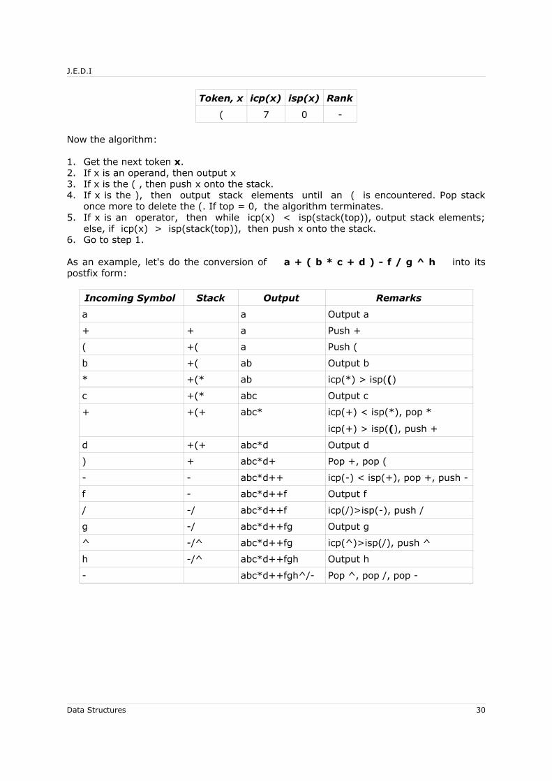
Token, x icp(x) isp(x) Rank

Operand 0 - +1

+ - 1 2 -1

* / 3 4 -1

^ 6 5 -1

Data Structures 29

J.E.D.I

Token, x icp(x) isp(x) Rank

( 7 0 -

Now the algorithm:

1. Get the next token x.2. If x is an operand, then output x3. If x is the ( , then push x onto the stack.4. If x is the ), then output stack elements until an ( is encountered. Pop stack

once more to delete the (. If top = 0, the algorithm terminates.5. If x is an operator, then while icp(x) < isp(stack(top)), output stack elements;

else, if icp(x) > isp(stack(top)), then push x onto the stack.6. Go to step 1.

As an example, let's do the conversion of a + ( b * c + d ) - f / g ^ h into its postfix form:

Incoming Symbol Stack Output Remarks

a a Output a

+ + a Push +

( +( a Push (

b +( ab Output b

* +(* ab icp(*) > isp(()

c +(* abc Output c

+ +(+ abc* icp(+) < isp(*), pop *

icp(+) > isp((), push +

d +(+ abc*d Output d

) + abc*d+ Pop +, pop (

- - abc*d++ icp(-) < isp(+), pop +, push -

f - abc*d++f Output f

/ -/ abc*d++f icp(/)>isp(-), push /

g -/ abc*d++fg Output g

^ -/^ abc*d++fg icp(^)>isp(/), push ^

h -/^ abc*d++fgh Output h

- abc*d++fgh^/- Pop ^, pop /, pop -

Data Structures 30

J.E.D.I

2.7 Advanced Topics on Stacks

2.7.1 Multiple Stacks using One-Dimensional Array

Two or more stacks may coexist in a common vector S of size n. This approach boasts of better memory utilization.

If two stacks share the same vector S, they grow toward each other with their bottoms anchored at opposite ends of S. The following figure shows the behavior of two stacks coexisting in a vector S:

Figure 1.11 Two Stacks Coexisting in a Vector

At initialization, stack 1's top is set to -1, that is, top1=-1 and for stack2 it is top2=n.

2.7.1.1 Three or More Stacks in a Vector S

If three or more stacks share the same vector, there is a need to keep track of several tops and base addresses. Base pointers defines the start of m stacks in a vector S with size n. Notation of which is B(i):

B[i] = n/m * i - 1 0 ≤ i < mB[m] = n-1

B[i] points to the space one cell below the stack's first actual cell. To initialize the stack, tops are set to point to base addresses, i.e.,

T[i] = B[i] , 0 ≤ i ≤ m

For example:

Three Stacks in a Vector

Data Structures 31

J.E.D.I

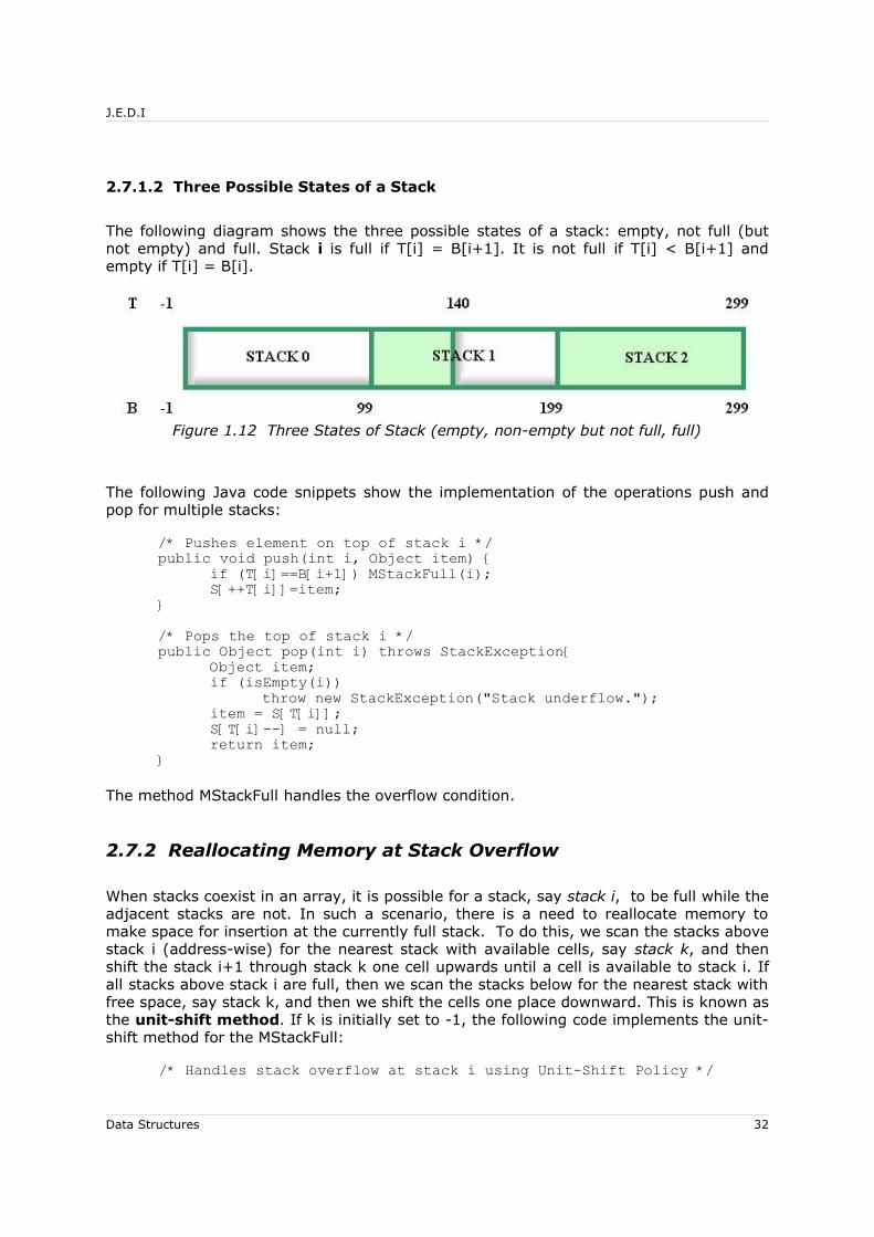
2.7.1.2 Three Possible States of a Stack

The following diagram shows the three possible states of a stack: empty, not full (but not empty) and full. Stack i is full if T[i] = B[i+1]. It is not full if T[i] < B[i+1] and empty if T[i] = B[i].

Figure 1.12 Three States of Stack (empty, non-empty but not full, full)

The following Java code snippets show the implementation of the operations push and pop for multiple stacks:

/* Pushes element on top of stack i */public void push(int i, Object item) {

if (T[i]==B[i+1]) MStackFull(i);S[++T[i]]=item;

}/* Pops the top of stack i */public Object pop(int i) throws StackException{

Object item;if (isEmpty(i))

throw new StackException("Stack underflow.");item = S[T[i]];S[T[i]--] = null;return item;

}

The method MStackFull handles the overflow condition.

2.7.2 Reallocating Memory at Stack Overflow

When stacks coexist in an array, it is possible for a stack, say stack i, to be full while the adjacent stacks are not. In such a scenario, there is a need to reallocate memory to make space for insertion at the currently full stack. To do this, we scan the stacks above stack i (address-wise) for the nearest stack with available cells, say stack k, and then shift the stack i+1 through stack k one cell upwards until a cell is available to stack i. If all stacks above stack i are full, then we scan the stacks below for the nearest stack with free space, say stack k, and then we shift the cells one place downward. This is known as the unit-shift method. If k is initially set to -1, the following code implements the unit-shift method for the MStackFull:

/* Handles stack overflow at stack i using Unit-Shift Policy */

Data Structures 32

J.E.D.I

/* Returns true if successful, otherwise false */void unitShift(int i) throws StackException{

int k=-1; /* Points to the 'nearest' stack with free space*//*Scan the stacks above(address-wise) the overflowed stack*/for (int j=i+1; j<m; j++)

if (T[j] < B[j+1]) {k = j;break;

}/* Shift the items of stack k to make room at stack i */if (k > i){

for (int j=T[k]; j>T[i]; j--)S[j+1] = S[j];

/* Adjust top and base pointers */for (int j=i+1; j<=k; j++) {

T[j]++;B[j]++;

}}/*Scan the stacks below if none is found above */else if (k > 0){

for (int j=i-1; j>=0; j--)if (T[j] < B[j+1]) {

k = j+1;break;

}for (int j=B[k]; j<=T[i]; j++)

S[j-1] = S[j];/* Adjust top and base pointers */for (int j=i; j>k; j--) {

T[j]--;B[j]--;

}}else /* Unsuccessful, every stack is full */

throw new StackException("Stack overflow.");}

2.7.2.1 Memory Reallocation using Garwick's Algorithm

Garwick's algorithm is a better way than unit-shift method to reallocate space when a stack becomes full. It reallocates memory in two steps: first, a fixed amount of space is divided among all the stacks; and second, the rest of the space is distributed to the stacks based on the current need. The following is the algorithm:

1. Strip all the stacks of unused cells and consider all of the unused cells as comprising the available or free space.

2. Reallocate one to ten percent of the available space equally among the stacks.3. Reallocate the remaining available space among the stacks in proportion to recent

growth, where recent growth is measured as the difference T[j] – oldT[j], where oldT[j] is the value of T[j] at the end of last reallocation. A negative(positive) difference means that stack j actually decreased(increased) in size since last reallocation.

Data Structures 33

J.E.D.I

Knuth's Implementation of Garwick's Algorithm

Knuth's implementation fixes the portion to be distributed equally among the stacks at 10%, and the remaining 90% are partitioned according to recent growth. The stack size (cumulative growth) is also used as a measure of the need in distributing the remaining 90%.The bigger the stack, the more space it will be allocated.

The following is the algorithm:

1. Gather statistics on stack usage

stack sizes = T[j] - B[j]Note: +1 if the stack that overflowed

differences = T[j] – oldT[j] if T[j] – oldT[j] >0 else 0 [Negative diff is replaced with 0]

Note: +1 if the stack that overflowed

freecells = total size – (sum of sizes)

incr = (sum of diff)

Note: +1 accounts for the cell that the overflowed stack is in need of.

2. Calculate the allocation factors

α = 10% * freecells / mβ = 90%* freecells / incr

where• m = number of stacks• α is the number of cells that each stack gets from 10% of available

space allotted• β is number of cells that the stack will get per unit increase in stack

usage from the remaining 90% of free space

3. Compute the new base addresses

σ - free space theoretically allocated to stacks 0, 1, 2, ..., j - 1τ - free space theoretically allocated to stacks 0, 1, 2, ..., j

actual number of whole free cells allocated to stack j = τ - σ

Initially, (new)B[0] = -1 and σ = 0

for j = 1 to m-1:τ = σ + α + diff[j-1]*βB[j] = B[j-1] + size[j-1] + τ - σ σ = τ

4. Shift stacks to their new boundaries

5. Set oldT = T

Data Structures 34

J.E.D.I

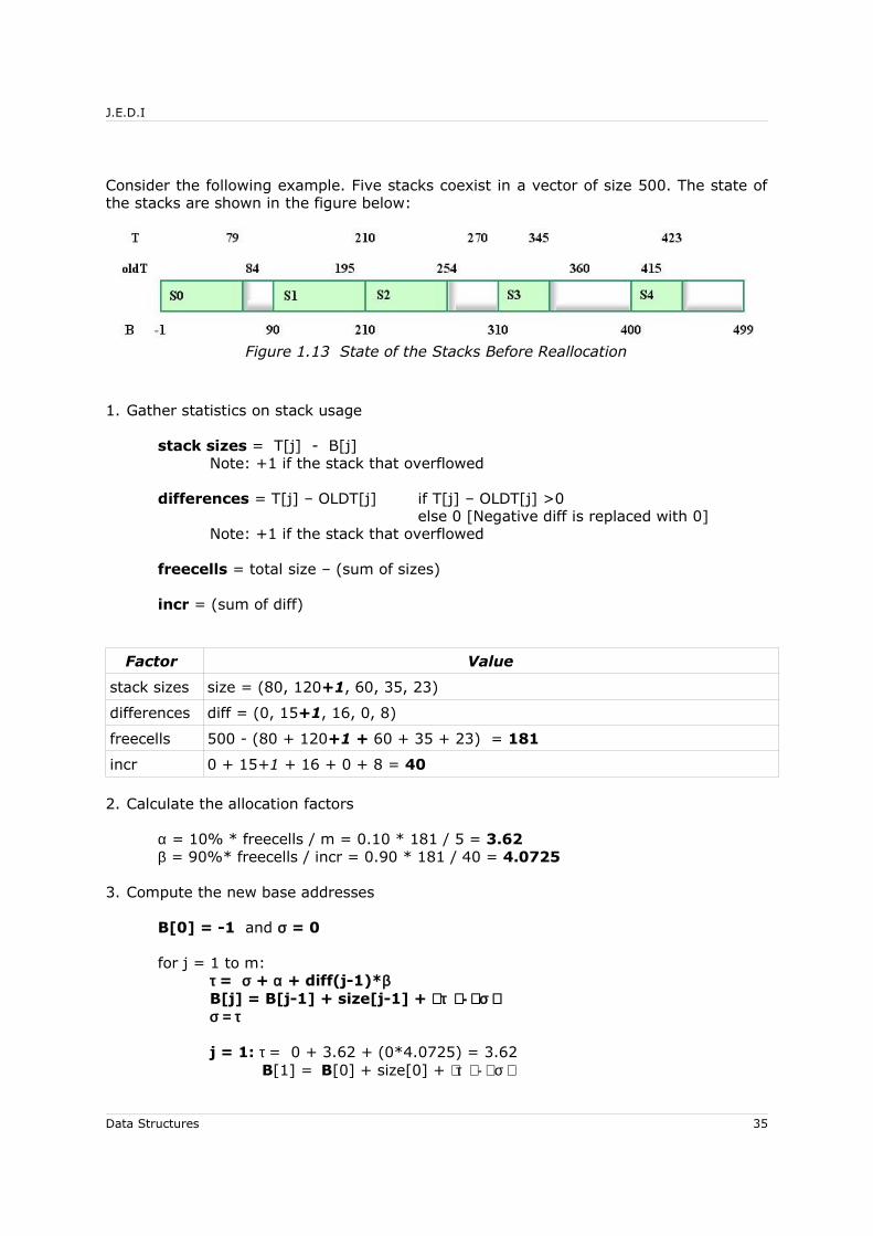
Consider the following example. Five stacks coexist in a vector of size 500. The state of the stacks are shown in the figure below:

Figure 1.13 State of the Stacks Before Reallocation

1. Gather statistics on stack usage

stack sizes = T[j] - B[j]Note: +1 if the stack that overflowed

differences = T[j] – OLDT[j] if T[j] – OLDT[j] >0 else 0 [Negative diff is replaced with 0]

Note: +1 if the stack that overflowed

freecells = total size – (sum of sizes)

incr = (sum of diff)

Factor Value

stack sizes size = (80, 120+1, 60, 35, 23)

differences diff = (0, 15+1, 16, 0, 8)

freecells 500 - (80 + 120+1 + 60 + 35 + 23) = 181

incr 0 + 15+1 + 16 + 0 + 8 = 40

2. Calculate the allocation factors

α = 10% * freecells / m = 0.10 * 181 / 5 = 3.62β = 90%* freecells / incr = 0.90 * 181 / 40 = 4.0725

3. Compute the new base addresses

B[0] = -1 and σ = 0

for j = 1 to m:τ = σ + α + diff(j-1)*βB[j] = B[j-1] + size[j-1] + τ - σ σ = τ

j = 1: τ = 0 + 3.62 + (0*4.0725) = 3.62B[1] = B[0] + size[0] + τ - σ

Data Structures 35

J.E.D.I

= -1 + 80 + 3.62 – 0 = 82σ = 3.62

j = 2: τ = 3.62 + 3.62 + (16*4.0725) = 72.4B[2] = B[1] + size[1] + τ - σ

= 82 + 121 + 72.4 – 3.62 = 272σ = 72.4

j = 3: τ = 72.4 + 3.62 + (16*4.0725) = 141.18B[3] = B[2] + size[2] + τ - σ

= 272 + 60 + 141.18 – 72.4 = 401σ = 141.18

j = 4: τ = 141.18 + 3.62 + (0*4.0725) = 144.8B[4] = B[3] + size[3] + τ - σ

= 401 + 35 + 144.8 – 141.18 = 439σ = 144.8

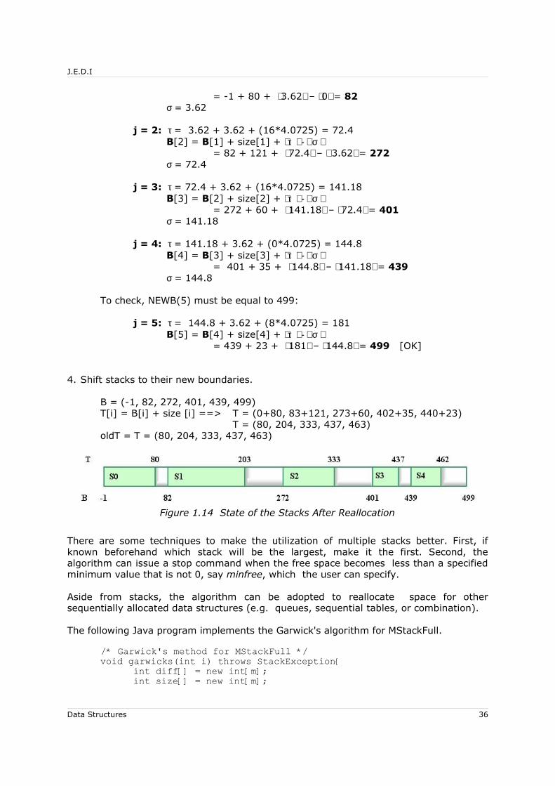
To check, NEWB(5) must be equal to 499:

j = 5: τ = 144.8 + 3.62 + (8*4.0725) = 181B[5] = B[4] + size[4] + τ - σ

= 439 + 23 + 181 – 144.8 = 499 [OK]

4. Shift stacks to their new boundaries.

B = (-1, 82, 272, 401, 439, 499)T[i] = B[i] + size [i] ==> T = (0+80, 83+121, 273+60, 402+35, 440+23)

T = (80, 204, 333, 437, 463)oldT = T = (80, 204, 333, 437, 463)

Figure 1.14 State of the Stacks After Reallocation

There are some techniques to make the utilization of multiple stacks better. First, if known beforehand which stack will be the largest, make it the first. Second, the algorithm can issue a stop command when the free space becomes less than a specified minimum value that is not 0, say minfree, which the user can specify.

Aside from stacks, the algorithm can be adopted to reallocate space for other sequentially allocated data structures (e.g. queues, sequential tables, or combination).

The following Java program implements the Garwick's algorithm for MStackFull.

/* Garwick's method for MStackFull */void garwicks(int i) throws StackException{

int diff[] = new int[m];int size[] = new int[m];

Data Structures 36

J.E.D.I

int totalSize = 0;double freecells, incr = 0;double alpha, beta, sigma=0, tau=0;/* Compute for the allocation factors */for (int j=0; j<m; j++){

size[j] = T[j]-B[j];if ( (T[j]-oldT[j]) > 0 ) diff[j] = T[j]-oldT[j];else diff[j] = 0;totalSize += size[j];incr += diff[j];

}diff[i]++;size[i]++;totalSize++;incr++;freecells = n - totalSize;alpha = 0.10 * freecells / m;beta = 0.90 * freecells / incr;/* If every stack is full */if (freecells < 1)

throw new StackException("Stack overflow.");/* Compute for the new bases */for (int j=1; j<m; j++){

tau = sigma + alpha + diff[j-1] * beta;B[j] = B[j-1] + size[j-1] + (int) Math.floor(tau)

- (int) Math.floor(sigma);sigma = tau;

}/* Restore size of the overflowed stack to its old value */size[i]--;/* Compute for the new top addresses */for (int j=0; j<m; j++) T[j] = B[j] + size[j];oldT = T;

}

2.8 Summary• A stack is a linearly ordered set of elements obeying the last-in, first-out (LIFO)

principle • Two basic stack operations are push and pop• Stacks have two possible implementations – a sequentially allocated one-

dimensional array (vector) or a linked linear list• Stacks are used in various applications such as pattern recognition, lists and tree

traversals, and evaluation of expressions• Two or more stacks coexisting in a common vector results in better memory

utilization• Memory reallocation techniques include the unit-shift method and Garwick's

algorithm

Data Structures 37

J.E.D.I


1. Infix to Postfix. Convert the following expressions into their infix form. Show the stack.

a) a+(b*c+d)-f/g^h

b) 1/2-5*7^3*(8+11)/4+2

2. Convert the following expressions into their postfix forma) a+b/c*d*(e+f)-g/hb) (a-b)*c/d^e*f^(g+h)-ic) 4^(2+1)/5*6-(3+7/4)*8-2d) (m+n)/o*p^q^r*(s/t+u)-v

Reallocation strategies for stack overflow. For numbers 3 and 4, a) draw a diagram showing the current state of the stacks.b) draw a diagram showing the state of the stacks after unit-shift policy is

implemented.c) draw a diagram showing the state of the stacks after the Garwick's algorithm is

used. Show how the new base addresses are computed.

3. Five stacks coexist in a vector of size 500. An insertion is attempted at stack 2. The state of computation is defined by:

OLDT(0:4) = (89, 178, 249, 365, 425)T(0:4) = (80, 220, 285, 334, 433)B(0:5) = (-1, 99, 220, 315, 410, 499)

4. Three stacks coexist in a vector of size 300. An insertion is attempted at stack 3. The state of computation is defined by:

OLDT(0:2) = (65, 180, 245)T(0:2) = (80, 140, 299)B(0:3) = (-1, 101, 215, 299)

2.10 Programming Exercises

1. Write a Java program that checks if parentheses and brackets are balanced in an arithmetic expression.

2. Create a Java class that implements the conversion of well-formed infix expression into its postfix equivalent.

3. Implement the conversion from infix to postfix expression using linked implementation of stack. The program shall ask input from the user and checks if the input is correct. Show the output and contents of the stack at every iteration.

4. Create a Java class definition of a multiple-stack in one dimensional vector.

Data Structures 38

J.E.D.I

Implement the basic operations on stack (push, pop, etc) to make them applicable on multiple-stack. Name the class MStack.

5. A book shop has bookshelves with adjustable dividers. When one divider becomes full, the divider could be adjusted to make space. Create a Java program that will reallocate bookshelf space using Garwick's Algorithm.

Data Structures 39

J.E.D.I

3 Queues

3.1 Objectives


• Define the basic concepts and operations on the ADT queue

• Implement the ADT queue using sequential and linked representation

• Perform operations on circular queue

• Use topological sorting in producing an order of elements satisfying a given

partial order

3.2 Introduction

A queue is a linearly ordered set of elements that has the discipline of First-In, First-Out. Hence, it is also known as a FIFO list.

There are two basic operations in queues: (1) insertion at the rear, and (2) deletion at the front.

To define the ADT queue in Java, we have the following interface:

interface Queue{/* Insert an item */void enqueue(Object item) throws QueueException;/* Delete an item */Object dequeue() throws QueueException;

}

Just like in stack, we will make use of the following exception:

class QueueException extends RuntimeException{public QueueException(String err){

super(err);}

}

3.3 Representation of Queues

Just like stack, queue may also be implemented using sequential representation or linked allocation.

Data Structures 40

J.E.D.I

3.3.1 Sequential Representation

If the implementation uses sequential representation, a one-dimensional array/vector is used, hence the size is static. The queue is empty if the front = rear and full if front=0 and rear=n. If the queue has data, front points to the actual front, while rear points to the cell after the actual rear. Deletion from an empty queue causes an underflow while insertion onto a full queue causes an overflow. The following figure shows an example of the ADT queue:

Figure 1.15 Operations on a Queue

Figure 1.16

To initialize, we set front and rear to 0:

front = 0;rear = 0;

To insert an item, say x, we do the following:

Q[rear] = item;rear++;

and to delete an item, we do the following:

x = Q[front];front++;

To implement a queue using sequential representation:

class SequentialQueue implements Queue{Object Q[];int n = 100 ; /* size of the queue, default 100 */int front = 0; /* front and rear set to 0 initially */int rear = 0;/* Create a queue of default size 100 */SequentialQueue1(){

Q = new Object[n];}/* Create a queue of the given size */SequentialQueue1(int size){

n = size;

Data Structures 41

J.E.D.I

Q = new Object[n];}/* Inserts an item onto the queue */public void enqueue(Object item) throws QueueException{

if (rear == n) throw new QueueException("Inserting into a full queue.");

Q[rear] = item;rear++;

}/* Deletes an item from the queue */public Object dequeue() throws QueueException{

if (front == rear) throw new QueueException("Deleting from an empty queue.");

Object x = Q[front];front++;return x;

}}

Whenever deletion is made, there is space vacated at the “front-side” of the queue. Hence, there is a need to move the items to make room at the “rear-side” for future insertion. The method moveQueue implements this procedure. This could be invoked when

void moveQueue() throws QueueException{if (front==0) throw new

QueueException("Inserting into a full queue");for(int i=front; i<n; i++)

Q[i-front] = Q[i];rear = rear - front;front = 0;

}

There is a need to modify the implementation of enqueue to make use of moveQueue:

public void enqueue(Object item){/* if rear is at the end of the array */if (rear == n) moveQueue(); Q[rear] = item;rear++;

}

3.3.2 Linked Representation

Linked allocation may also be used to represent a queue. It also makes use of nodes with fields INFO and LINK. The following figure shows a queue implemented as a linked list:

Figure 1.17 Linked Representation of a Queue

Data Structures 42

J.E.D.I

The node definition in chapter 1 will also be used here.

The queue is empty if front = null. In linked representation, since the queue grows dynamically, overflow will happen only when the program runs out of memory and dealing with that is beyond the scope of this topic.

The following Java code implements the linked representation of the ADT queue:

class LinkedQueue implements Queue{queueNode front, rear;/* Create an empty queue */LinkedQueue(){}/* Create a queue with node n initially */LinkedQueue(queueNode n){

front = n;rear = n;

}/* Inserts an item onto the queue */public void enqueue(Object item){

queueNode n = new queueNode(item, null);if (front == null) {

front = n;rear = n;

}else{

rear.link = n;rear = n;

}}/* Deletes an item from the queue */public Object dequeue() throws QueueException{

Object x;if (front == null) throw new QueueException

("Deleting from an empty queue.");x = front.info;front = front.link;return x;

}}

3.4 Circular Queue

A disadvantage of the previous sequential implementation is the need to move the elements, in the case of rear = n and front > 0, to make room for insertion. If queues are viewed as circular instead, there will be no need to perform such move. In a circular queue, the cells are considered arranged in a circle. The front points to the actual element at the front of the queue while the rear points to the cell on the right of the actual rear element (clockwise). The following figure shows a circular queue:

Data Structures 43

J.E.D.I

Figure 1.18 Circular Queue

Figure 1.19

To initialize a circular queue:front = 0; rear = 0;

To insert an item, say x:Q[rear] = x;rear = (rear + 1) mod n;

To delete:

x = Q[front];front = (front + 1) mod n;

We use the modulo function instead of performing an if test in incrementing rear and front. As insertions and deletions are done, the queue moves in a clockwise direction. If front catches up with rear, i.e., if front = rear, then we get an empty queue. If rear catches up with front, a condition also indicated by front = rear, then all cells are in use and we get a full queue. In order to avoid having the same relation signify two different conditions, we will not allow rear to catch up with front by considering the queue as full when exactly one free cell remains. Thus a full queue is indicated by:

front == (rear + 1) mod n

The following methods are implementations of inserting into and deleting from a circular queue:

Data Structures 44

J.E.D.I

public void enqueue(Object item) throws QueueException{if (front == (rear % n) + 1) throw new QueueException(

"Inserting into a full queue.");Q[rear] = item;rear = (rear % n) + 1;

}public Object dequeue() throws QueueException{

Object x;if (front == rear) throw new QueueException(

"Deleting from an empty queue.");x = Q[front];front = (front % n) + 1;return x;

}

3.5 Application: Topological Sorting

Topological sorting is problem involving activity networks. It uses both sequential and link allocation techniques in which the linked queue is embedded in a sequential vector.

It is a process applied to partially ordered elements. The input is a set of pairs of partial ordering and the output is the list of elements, in which there is no element listed with its predecessor not yet in the output.

Partial ordering is defined as a relation between the elements of set S, denoted by ≼ which is read as 'precedes or equals'. The following are the properties of partial ordering ≼:

• Transitivity : if x ≼ y and y ≼ z, then x ≼ z.• Antisymmetry : if x ≼ y and y ≼ x, the x = y.• Reflexivity : x ≼ x.

Corollaries. If x ≼ y and x ≠ y then x ≺ y. Equivalent set of properties are:

• Transitivity : if x ≺ y and y ≺ z, then x ≺ z.• Asymmetry : if x ≺ y then y ≺ x.• Irreflexivity : x ≺x.

A familiar example of partial ordering from mathematics is the relation u ⊆ v between sets u and v. The following is another example where the list of partial ordering is shown on the left; the graph that illustrates the partial ordering is shown at the center, and the expected output is shown at the right.

Data Structures 45

J.E.D.I

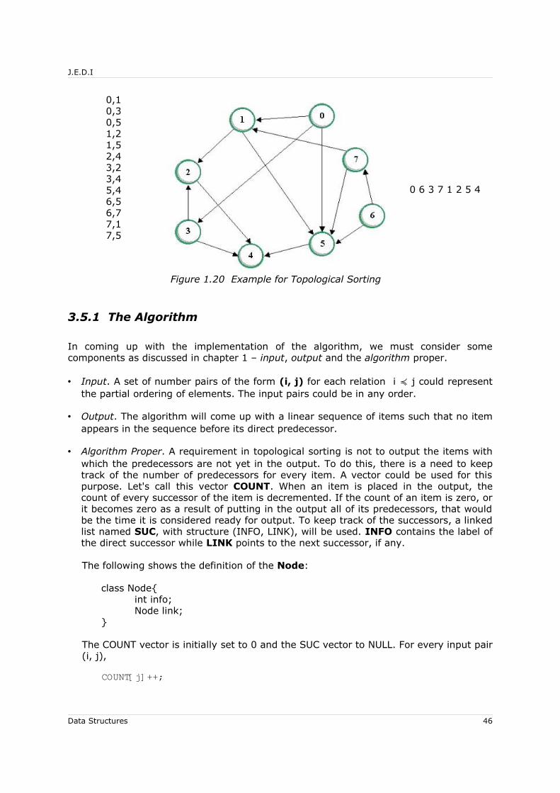
0,10,30,51,21,52,43,23,45,46,56,77,17,5

Figure 1.20 Example for Topological Sorting

0 6 3 7 1 2 5 4

3.5.1 The Algorithm

In coming up with the implementation of the algorithm, we must consider some components as discussed in chapter 1 – input, output and the algorithm proper.

• Input. A set of number pairs of the form (i, j) for each relation i ≼ j could represent the partial ordering of elements. The input pairs could be in any order.

• Output. The algorithm will come up with a linear sequence of items such that no item appears in the sequence before its direct predecessor.

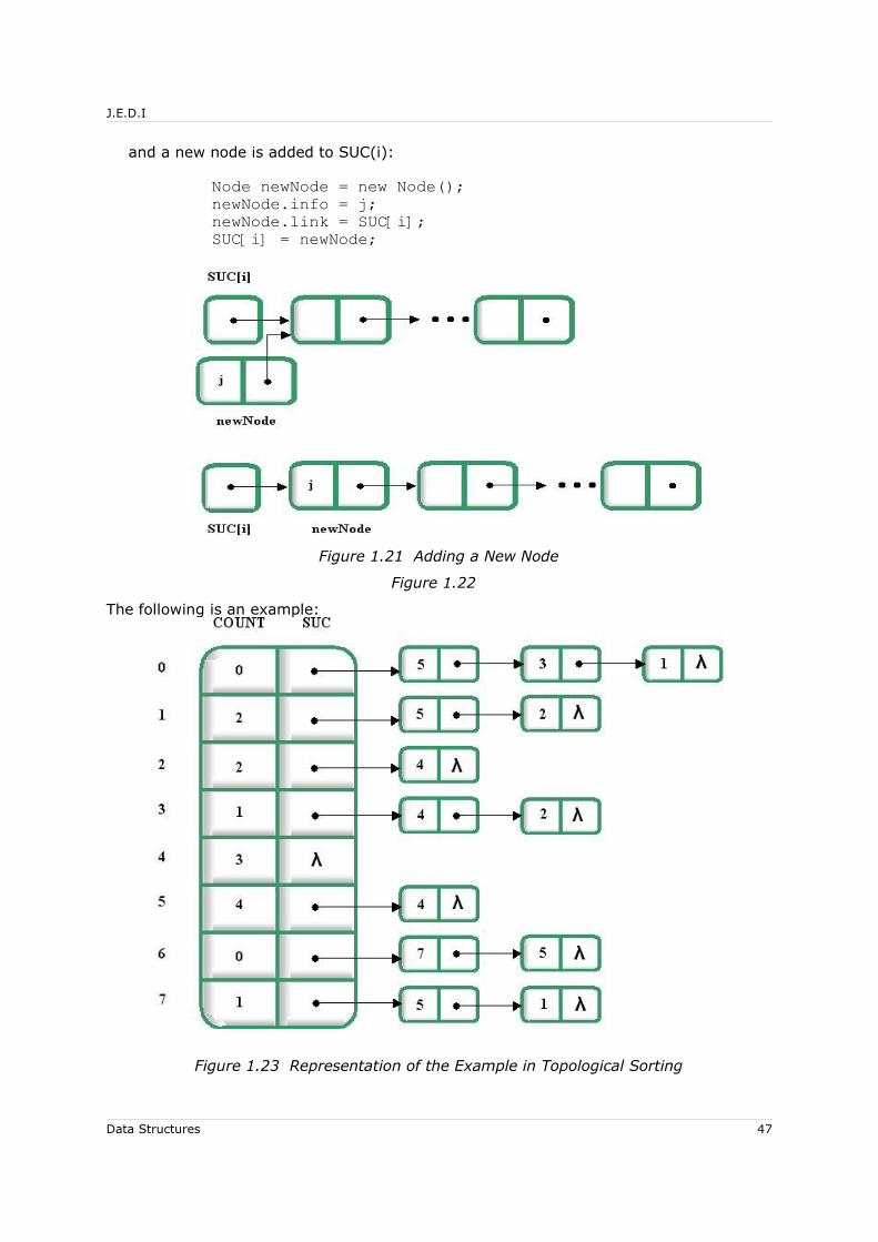
• Algorithm Proper. A requirement in topological sorting is not to output the items with which the predecessors are not yet in the output. To do this, there is a need to keep track of the number of predecessors for every item. A vector could be used for this purpose. Let's call this vector COUNT. When an item is placed in the output, the count of every successor of the item is decremented. If the count of an item is zero, or it becomes zero as a result of putting in the output all of its predecessors, that would be the time it is considered ready for output. To keep track of the successors, a linked list named SUC, with structure (INFO, LINK), will be used. INFO contains the label of the direct successor while LINK points to the next successor, if any.

The following shows the definition of the Node:

class Node{int info;Node link;

}

The COUNT vector is initially set to 0 and the SUC vector to NULL. For every input pair (i, j),

COUNT[j]++;

Data Structures 46

J.E.D.I

and a new node is added to SUC(i):

Node newNode = new Node();newNode.info = j;newNode.link = SUC[i];SUC[i] = newNode;

Figure 1.21 Adding a New Node

Figure 1.22

The following is an example:

Figure 1.23 Representation of the Example in Topological Sorting

Data Structures 47

J.E.D.I

Figure 1.24

Figure 1.25

To generate the output, which is a linear ordering of the objects such that no object appears in the sequence before its direct predecessors, we proceed as follows:

1. Look for an item, say k, with count of direct predecessors equal to zero, i.e., COUNT[k] == 0. Put k in the output.

2. Scan list of direct successors of k, and decrement the count of each such successor by 1.

3. Repeat steps 1 and 2 until all items are in the output.

To avoid having to go through the COUNT vector repeatedly as we look for objects with a count of zero, we will constitute all such objects into a linked queue. Initially, the queue will consist of items with no direct predecessors (there will always be at least one such item). Subsequently, each time that the count of direct predecessors of an item drops to zero, it is inserted into the queue, ready for output. Since for each item, say j, in the queue, the count is zero, we can now reuse COUNT[j] as a link field such that

COUNT[j] = k if k is the next item in the queue

= 0 if j is the rear element in the queue

Hence, we have an embedded linked queue in a sequential vector.

If the input to the algorithm is correct, i.e., if the input relations satisfy partial ordering, then the algorithm terminates when the queue is empty with all n objects placed in the output. If, on the other hand, partial ordering is violated such that there are objects which constitute one or more loops (for instance, 1≺2; 2≺3; 3≺4; 4≺1), then the algorithm still terminates, but objects comprising a loop will not be placed in the output.

This approach of topological sorting uses both sequential and linked allocation techniques, and the use of a linked queue that is embedded in a sequential vector.

3.6 Summary• A queue is a linearly ordered set of elements obeying the first-in, first-out (FIFO)

principle

• Two basic queue operations are insertion at the rear and deletion at the front

• Queues have 2 implementations - sequential and linked

• In circular queues, there is no need to move the elements to make room for insertion

• The topological sorting approach discussed uses both sequential and linked allocation techniques, as well as a linked queue embedded in a sequential vector

Data Structures 48

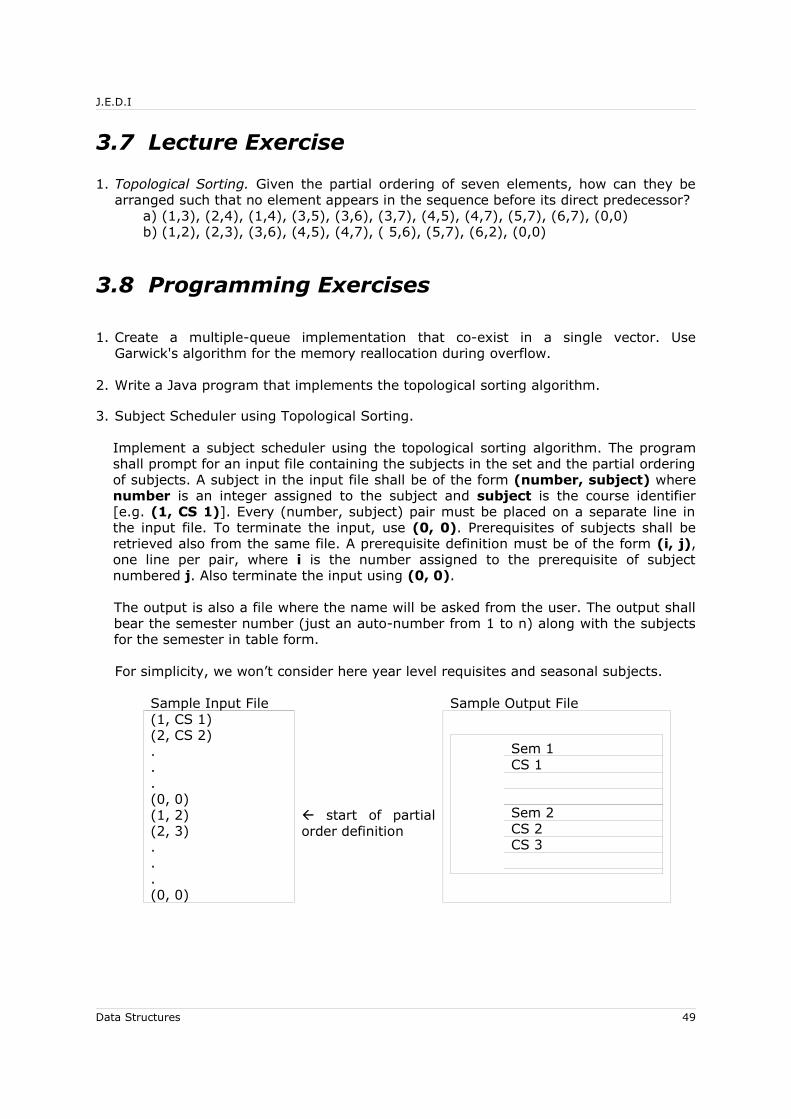
J.E.D.I

3.7 Lecture Exercise

1. Topological Sorting. Given the partial ordering of seven elements, how can they be arranged such that no element appears in the sequence before its direct predecessor?

a) (1,3), (2,4), (1,4), (3,5), (3,6), (3,7), (4,5), (4,7), (5,7), (6,7), (0,0)b) (1,2), (2,3), (3,6), (4,5), (4,7), ( 5,6), (5,7), (6,2), (0,0)


1. Create a multiple-queue implementation that co-exist in a single vector. Use Garwick's algorithm for the memory reallocation during overflow.

2. Write a Java program that implements the topological sorting algorithm.

3. Subject Scheduler using Topological Sorting.

Implement a subject scheduler using the topological sorting algorithm. The program shall prompt for an input file containing the subjects in the set and the partial ordering of subjects. A subject in the input file shall be of the form (number, subject) where number is an integer assigned to the subject and subject is the course identifier [e.g. (1, CS 1)]. Every (number, subject) pair must be placed on a separate line in the input file. To terminate the input, use (0, 0). Prerequisites of subjects shall be retrieved also from the same file. A prerequisite definition must be of the form (i, j), one line per pair, where i is the number assigned to the prerequisite of subject numbered j. Also terminate the input using (0, 0).

The output is also a file where the name will be asked from the user. The output shall bear the semester number (just an auto-number from 1 to n) along with the subjects for the semester in table form.

For simplicity, we won’t consider here year level requisites and seasonal subjects.

Sample Input File Sample Output File(1, CS 1)(2, CS 2)...(0, 0)(1, 2)(2, 3)...(0, 0)

start of partial order definition

Sem 1CS 1

Sem 2CS 2CS 3

Data Structures 49

J.E.D.I

4 Binary Trees

4.1 Objectives


• Explain the basic concepts and definitions related to binary trees

• Identify the properties of a binary tree

• Enumerate the different types of binary trees

• Discuss how binary trees are represented in computer memory

• Traverse binary trees using the three traversal algorithms: preorder, inorder, postorder

• Discuss binary tree traversal applications

• Use heaps and the heapsort algorithm to sort a set of elements

4.2 Introduction

Binary tree is an abstract data type that is hierarchical in structure. It is a collection of nodes which are either empty or consists of a root and two disjoint binary trees called the left and the right subtrees. It is similar to a tree in the sense that there is the concept of a root, leaves and branches. However, they differ in orientation since the root of a binary tree is the topmost element, in contrast to the bottommost element in a real tree.

Binary tree is most commonly used in searching, sorting, efficient encoding of strings, priority queues, decision tables and symbol tables.

4.3 Definitions and Related Concepts

A binary tree T has a special node, say r, which is called the root. Each node v of T that is different from r, has a parent node p. Node v is said to be a child (or son) of node p. A node can have at least zero (0) and at most two (2) children that can be classified as a left child/son or right child/son. The subtree of T rooted at node v is the tree that has node v's children as its root. It is a left subtree if it is rooted at the left son of node v or a right subtree if it is rooted at the right son of node v. The number of non-null subtrees of a node is called its degree. If a node has degree zero, it is classified as a leaf or a terminal node.

Data Structures 50

J.E.D.I

Figure 1.26 A Binary Tree

Level of a node refers to the distance of the node from the root. Hence, the root of the tree has level 0, its subtrees at level 1 and so on. The height or depth of a tree is the level of the bottommost nodes, which is also the length of the longest path from the root to any leaf. For example, the following binary tree has a height of 3:

Figure 1.27 Levels of a Binary Tree

Figure 1.28

A node is external if it has no children, otherwise it is internal. If two nodes have the same parents, they are said to be siblings. Ancestor of a node is either the node itself or ancestor of its parent. Conversely, a node u is a descendant of a node v if v is an ancestor of node u.

Data Structures 51

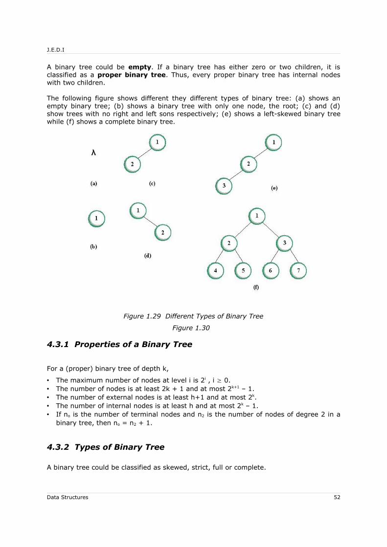
J.E.D.I

A binary tree could be empty. If a binary tree has either zero or two children, it is classified as a proper binary tree. Thus, every proper binary tree has internal nodes with two children.

The following figure shows different they different types of binary tree: (a) shows an empty binary tree; (b) shows a binary tree with only one node, the root; (c) and (d) show trees with no right and left sons respectively; (e) shows a left-skewed binary tree while (f) shows a complete binary tree.

Figure 1.29 Different Types of Binary Tree

Figure 1.30

4.3.1 Properties of a Binary Tree

For a (proper) binary tree of depth k,

• The maximum number of nodes at level i is 2i , i ≥ 0.• The number of nodes is at least 2k + 1 and at most 2k+1 – 1.• The number of external nodes is at least h+1 and at most 2k.• The number of internal nodes is at least h and at most 2k – 1.• If no is the number of terminal nodes and n2 is the number of nodes of degree 2 in a

binary tree, then no = n2 + 1.

4.3.2 Types of Binary Tree

A binary tree could be classified as skewed, strict, full or complete.

Data Structures 52

J.E.D.I

A right ( left ) skewed binary tree is a tree in which every node has no left (right)subtrees. For a given number of nodes, a left or right-skewed binary tree has the greatest depth.

A strictly binary tree is a tree in which every node has either two subtrees or none at all.

Figure 1.31 Left and Right-Skewed Binary Trees

Figure 1.32

Figure 1.33 Strictly Binary Tree

A full binary tree is a strictly binary tree in which all terminal nodes lie at the bottom-most level. For a given depth, this tree has the maximum number of nodes.

Data Structures 53

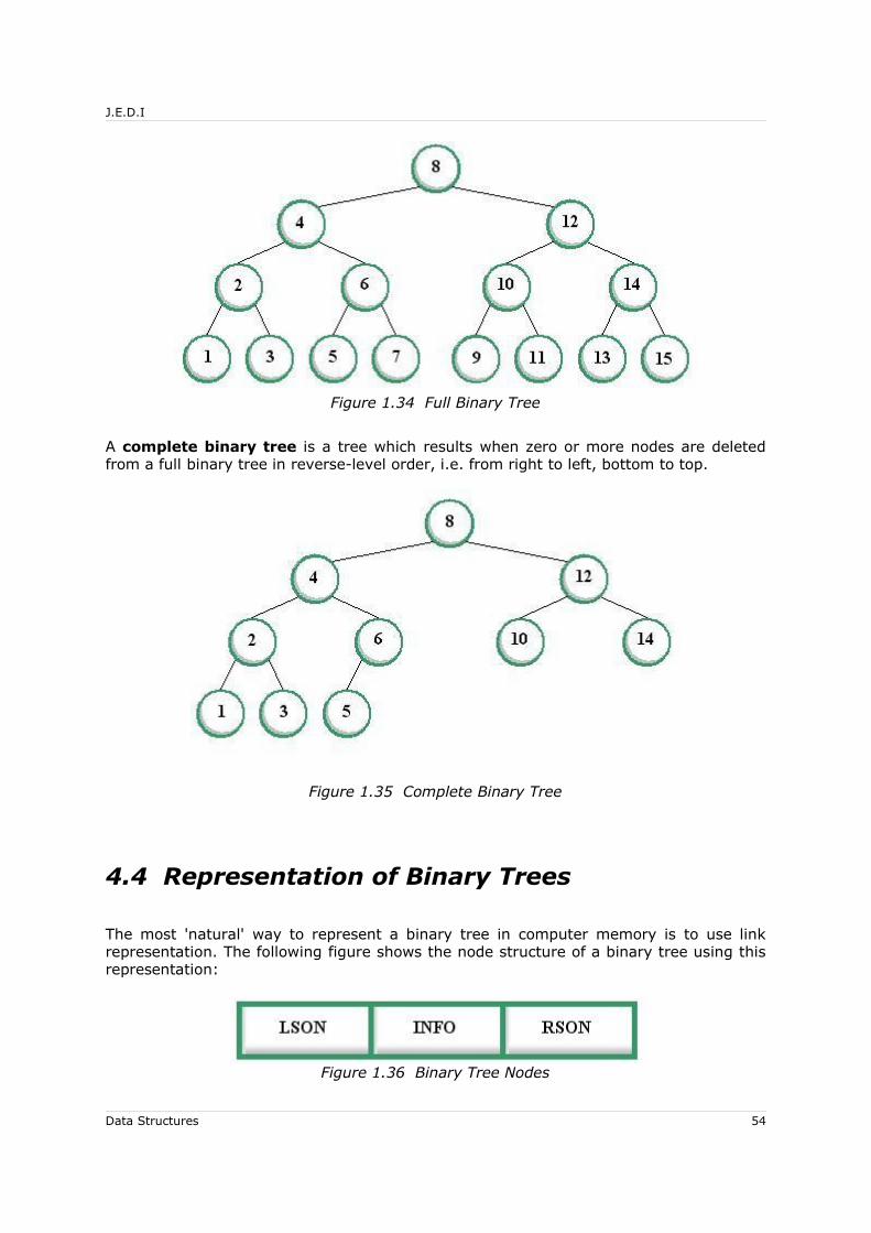
J.E.D.I

Figure 1.34 Full Binary Tree

A complete binary tree is a tree which results when zero or more nodes are deleted from a full binary tree in reverse-level order, i.e. from right to left, bottom to top.

Figure 1.35 Complete Binary Tree

4.4 Representation of Binary Trees

The most 'natural' way to represent a binary tree in computer memory is to use link representation. The following figure shows the node structure of a binary tree using this representation:

Figure 1.36 Binary Tree Nodes

Data Structures 54

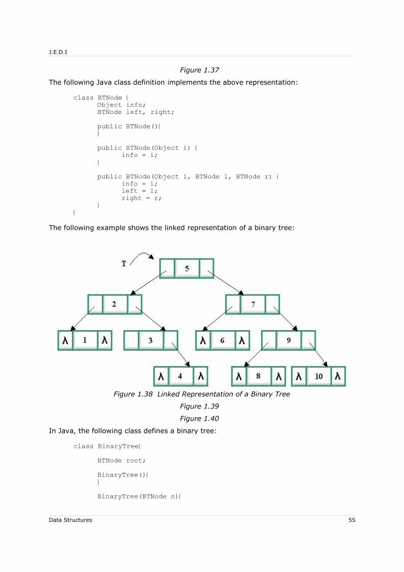
J.E.D.I

Figure 1.37

The following Java class definition implements the above representation:

class BTNode {Object info;BTNode left, right;public BTNode(){}public BTNode(Object i) {

info = i;}public BTNode(Object i, BTNode l, BTNode r) {

info = i;left = l;right = r;

}}

The following example shows the linked representation of a binary tree:

Figure 1.38 Linked Representation of a Binary Tree

Figure 1.39

Figure 1.40

In Java, the following class defines a binary tree:

class BinaryTree{BTNode root;BinaryTree(){}BinaryTree(BTNode n){

Data Structures 55

J.E.D.I

root = n;}BinaryTree(BTNode n, BTNode left, BTNode right){

root = n;root.left = left;root.right = right;

}}

4.5 Binary Tree Traversals

Computations in binary trees often involve traversals. Traversal is a procedure that visits the nodes of the binary tree in a linear fashion such that each node is visited exactly once, where visit is defined as performing computations local to the node.

There are three ways to traverse a tree: preorder, inorder, postorder. The prefix (pre, in and post) refers to the order in which the root of every subtree is visited.

4.5.1 Preorder Traversal

In preorder traversal of a binary tree, the root is visited first. Then the children are traversed recursively in the same manner. This traversal algorithm is useful for applications requiring listing of elements where the parents must always come before their children.

The Method:

If the binary tree is empty, do nothing (traversal done)Otherwise:

Visit the root.Traverse the left subtree in preorder.Traverse the right subtree in preorder.

Figure 1.41 Preorder Traversal

Figure 1.42

Data Structures 56

J.E.D.I

In Java, add the following method to class BinaryTree:

/* Outputs the preorder listing of elements in this tree */void preorder(){

if (root != null) {System.out.println(root.info.toString());new BinaryTree(root.left).preorder();new BinaryTree(root.right).preorder();

}}

4.5.2 Inorder Traversal

The inorder traversal of a binary tree can be informally defined as the “left-to-right” traversal of a binary tree. That is, the left subtree is recursively traversed in inorder, followed by a visit to its parent, then finished with recursive traversal of the right subtree also in inorder.

The Method:


Traverse the left subtree in inorder.Visit the root.Traverse the right subtree in inorder.

Figure 1.43 Inorder Traversal

Figure 1.44


/* Outputs the inorder listing of elements in this tree */void inorder(){

if (root != null) {new BinaryTree(root.left).inorder();System.out.println(root.info.toString());new BinaryTree(root.right).inorder();

Data Structures 57

J.E.D.I

}}

4.5.3 Postorder Traversal

Postorder traversal is the opposite of preorder, that is, it recursively traverses the children first before their parents.

The Method:


Traverse the left subtree in postorder.Traverse the right subtree in postorder.Visit the root.

Figure 1.45 Postorder Traversal

Figure 1.46


/* Outputs the postorder listing of elements in this tree */void postorder(){

if (root != null) {new BinaryTree(root.left).postorder();new BinaryTree(root.right).postorder();System.out.println(root.info.toString());

}}

The following are some examples:

Data Structures 58

J.E.D.I

Figure 1.47 Example 1

Figure 1.48

Figure 1.49 Example 2

Figure 1.50

Data Structures 59

J.E.D.I

4.6 Applications of Binary Tree Traversals

Binary tree traversals have several applications. In this section, two applications will be covered: duplication of a binary tree and checking equivalence of two binary trees.

4.6.1 Duplicating a Binary Tree

There are instances that a duplicate of an existing binary tree would be needed for computation. To do this, the following algorithm to copy an existing binary tree can be used:

1. Traverse the left subtree of node α in postorder and make a copy of it 2. Traverse the right subtree of node α in postorder and make a copy of it3. Make a copy of node α and attach copies of its left and right subtrees

The following Java method of the BinaryTree class implements copy:

/* Copies this tree and returns the root of the duplicate */BTNode copy(){

BTNode newRoot;BTNode newLeft;BTNode newRight;if (root != null){

newLeft = new BinaryTree(root.left).copy();newRight = new BinaryTree(root.right).copy();

newRoot = new BTNode(root.info, newLeft, newRight); return newRoot;

}return null;

}

4.6.2 Equivalence of Two Binary Trees

Two binary trees are equivalent if one is an exact duplicate of the other. The following is the algorithm to check equivalence of two binary trees:

1. Check whether node α and node α contain the same data2. Traverse the left subtrees of node α and node α in preorder and check whether

they are equivalent3. Traverse the right subtrees of node α and node α in preorder and check

whether they are equivalent

The following code snippet, which is a method of BinaryTree, implements this algorithm:

/* Compare another tree t2 if it's equivalent to this tree */boolean equivalent(BinaryTree t2){

boolean answer = false;if ((root == null) && (t2.root == null)) answer = true;else {

Data Structures 60

J.E.D.I

answer = (root.info.equals(t2.root.info));if (answer) answer =

new BinaryTree(root.left).equivalent(new BinaryTree(t2.root.left));

if (answer) answer = new BinaryTree(root.right).equivalent(

new BinaryTree(t2.root.right));}return answer;

}

4.7 Binary Tree Application: Heaps and the Heapsort Algorithm

A heap is defined as a complete binary tree that has elements stored at its nodes and satisfies the heap-order property. A complete binary tree, as defined in the previous lesson, results when zero or more nodes are deleted from a full binary tree in reverse level order. Hence, its leaves lie on at most two adjacent levels and the leaves at the bottommost level lie at the leftmost position of the complete binary tree.

The heap-order property states that for every node u except the root, the key stored at u is less than or equal to the key stored at its parent. Hence, the root always contain the maximum value.

In this application, the elements stored in a heap satisfy the total order. A total order is a relation between the elements of a set of objects, say S, satisfying the following properties for any objects x, y and z in S:

• Transitivity: if x < y and y < z then x < z.

• Trichotomy: for any two objects x and y in S, exactly one of these relations holds: x > y, x = y or x < y.

Data Structures 61

J.E.D.I

Figure 1.51 Two Representations of the elements a l g o r i t h m s

4.7.1 Sift-Up

A complete binary tree may be converted into a heap by applying a process called sift-up. In the process, larger keys “sift-up” the tree to make it satisfy the heap-order property. This is a bottom-up, right-to-left, process in which the smallest subtrees of a complete binary tree are converted into heaps, then the subtrees which contain them, and so on, until the entire binary tree is converted into a heap.

Note that when the subtree rooted at any node, say α, is converted into a heap, its left and right subtrees are already heaps. We call such a subtree an almost-heap. When an almost heap is converted into a heap, one of its subtrees may cease to be a heap (i.e., it may become an almost heap). This, however, may be converted to a heap and the process continues as smaller and yet smaller subtrees lose and regain the heap property, with LARGER keys migrating upwards.

4.7.2 Sequential Representation of a Complete Binary Tree

Data Structures 62

J.E.D.I

A complete binary tree may be represented sequentially in a one-dimensional vector of size n in level-order. If the nodes of a binary tree are numbered as illustrated below,

Figure 1.52 A complete Binary Tree

then it can be represented sequentially in a vector named KEY, as follows:

Figure 1.53 Sequential Representation of a Complete Binary Tree

Sequential representation of a complete binary tree enables locating the children (if any), the parent (if it exists) and the parent of a node in constant time by using the following formula:

• if 2i ≤ n, the left son of node i is 2i; otherwise, node i has no left son• if 2i + 1 ≤ n, the right son of node i is 2i + 1; otherwise, node i has no right

son• if 1 < i ≤ n, the father of node i is (i)/2

The following method implements the sift up process on sequentially represented complete binary tree:

/* Converts an almost-heap on n nodes rooted at i into a heap */private void siftUp (int i, int n) {

int k = key[i]; /* keep key at root of almost-heap */int child = 2 * i; /* left child */while (child <= n) {

/* if the right child is bigger, make the child pointto the right child */

if (child < n && key[child+1]> key[child]) child++ ;/* if heap property is not satisfied */if (key[child] > k){

key[i] = key[child] ; /* Move the child up */

Data Structures 63

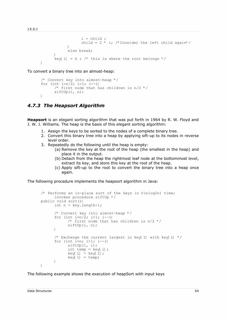
J.E.D.I

i = child ;child = 2 * i; /*Consider the left child again*/

}else break;

}key[i] = k ; /* this is where the root belongs */

}

To convert a binary tree into an almost-heap:

/* Convert key into almost-heap */for (int i=n/2; i>1; i--){

/* first node that has children is n/2 */siftUp(i, n);

}

4.7.3 The Heapsort Algorithm

Heapsort is an elegant sorting algorithm that was put forth in 1964 by R. W. Floyd and J. W. J. Williams. The heap is the basis of this elegant sorting algorithm:

1. Assign the keys to be sorted to the nodes of a complete binary tree.2. Convert this binary tree into a heap by applying sift-up to its nodes in reverse

level order.3. Repeatedly do the following until the heap is empty:

(a) Remove the key at the root of the heap (the smallest in the heap) and place it in the output.

(b) Detach from the heap the rightmost leaf node at the bottommost level, extract its key, and store this key at the root of the heap.

(c) Apply sift-up to the root to convert the binary tree into a heap once again.

The following procedure implements the heapsort algorithm in Java:

/* Performs an in-place sort of the keys in O(nlog2n) time; invokes procedure siftUp */

public void sort(){int n = key.length-1;/* Convert key into almost-heap */for (int i=n/2; i>1; i--){

/* first node that has children is n/2 */siftUp(i, n);

}/* Exchange the current largest in key[1] with key[i] */for (int i=n; i>1; i--){

siftUp(1, i);int temp = key[i];key[i] = key[1];key[1] = temp;

}}

The following example shows the execution of heapSort with input keys

Data Structures 64

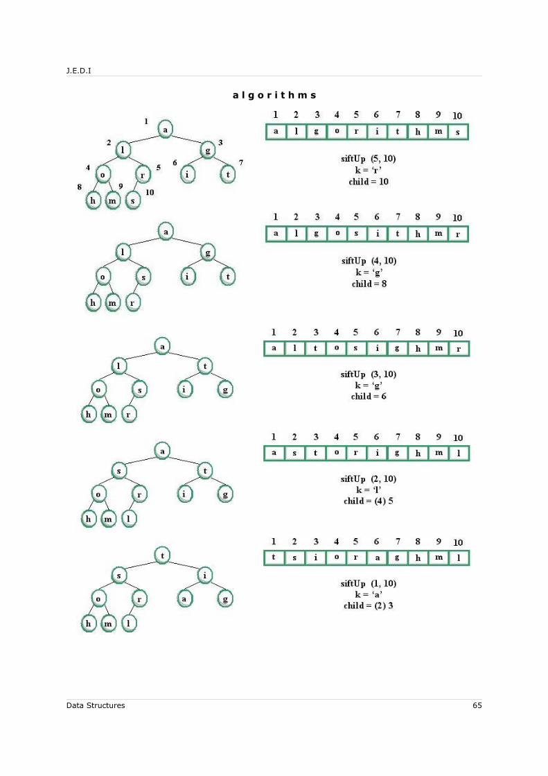
J.E.D.I

a l g o r i t h m s

Data Structures 65

J.E.D.I

Data Structures 66

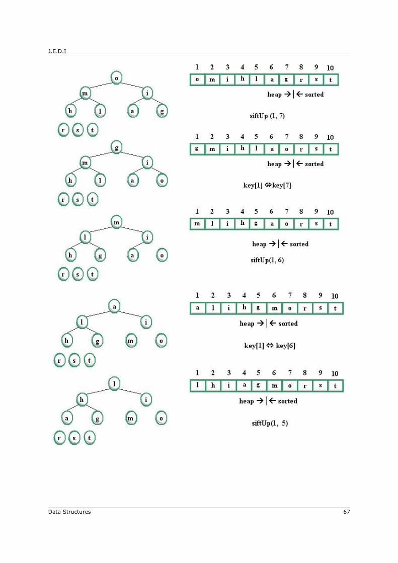
J.E.D.I

Data Structures 67

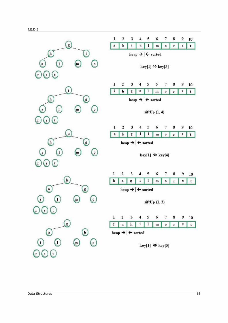
J.E.D.I

Data Structures 68

J.E.D.I

Figure 1.54 Heapsort Example

4.8 Summary

• A binary tree is an abstract data type that is hierarchical in structure

• A binary tree could be classified as skewed, strict, full or complete

• Link representation is the most natural way to represent a binary tree

• Three ways to traverse a tree are preorder, inorder, and postorder

• Binary tree traversals could be used in applications such as duplication of a binary tree and checking the equivalence of two binary trees

• The heapsort algorithm utilizes the heap ADT and runs in O(n lg n) time

Data Structures 69

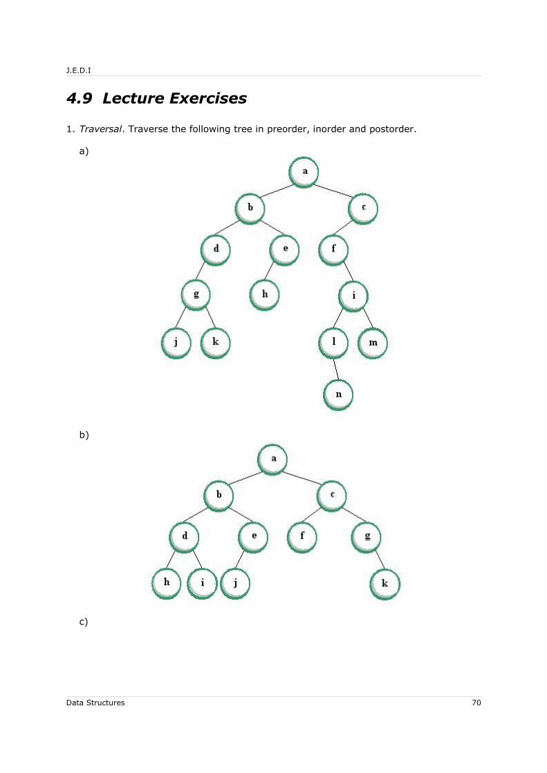
J.E.D.I


1. Traversal. Traverse the following tree in preorder, inorder and postorder.

a)

b)

c)

Data Structures 70

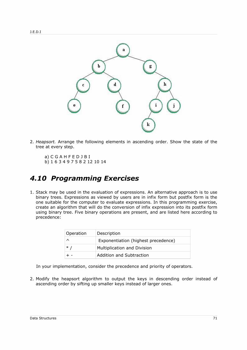
J.E.D.I

2. Heapsort. Arrange the following elements in ascending order. Show the state of the tree at every step.

a) C G A H F E D J B Ib) 1 6 3 4 9 7 5 8 2 12 10 14


1. Stack may be used in the evaluation of expressions. An alternative approach is to use binary trees. Expressions as viewed by users are in infix form but postfix form is the one suitable for the computer to evaluate expressions. In this programming exercise, create an algorithm that will do the conversion of infix expression into its postfix form using binary tree. Five binary operations are present, and are listed here according to precedence:

Operation Description

^ Exponentiation (highest precedence)

* / Multiplication and Division

+ - Addition and Subtraction

In your implementation, consider the precedence and priority of operators.

2. Modify the heapsort algorithm to output the keys in descending order instead of ascending order by sifting up smaller keys instead of larger ones.

Data Structures 71

J.E.D.I

5 Trees

5.1 Objectives


• Discuss the basic concepts and definitions on trees

• Identify the types of trees: ordered, oriented and free tree

• Use the link presentation of trees

• Explain the basic concepts and definitions on forests

• Convert a forest into its binary tree representation and vice versa using

natural correspondence

• Traverse forests using preorder, postorder, level-order and family-order

• Create representation of trees using sequential allocation

• Represent trees using arithmetic tree representations

• Use trees in an application: the equivalence problem


5.2.1 Ordered Tree

An ordered tree is a finite set, say T, of one or more nodes such that there is specially designated node called the root and the remaining roots are partitioned into n ≥ 0 disjoint sets T1, T2, ... , Tn, where each of these sets is an ordered tree. In an ordered tree, the order of each node in the tree is significant.

Data Structures 72

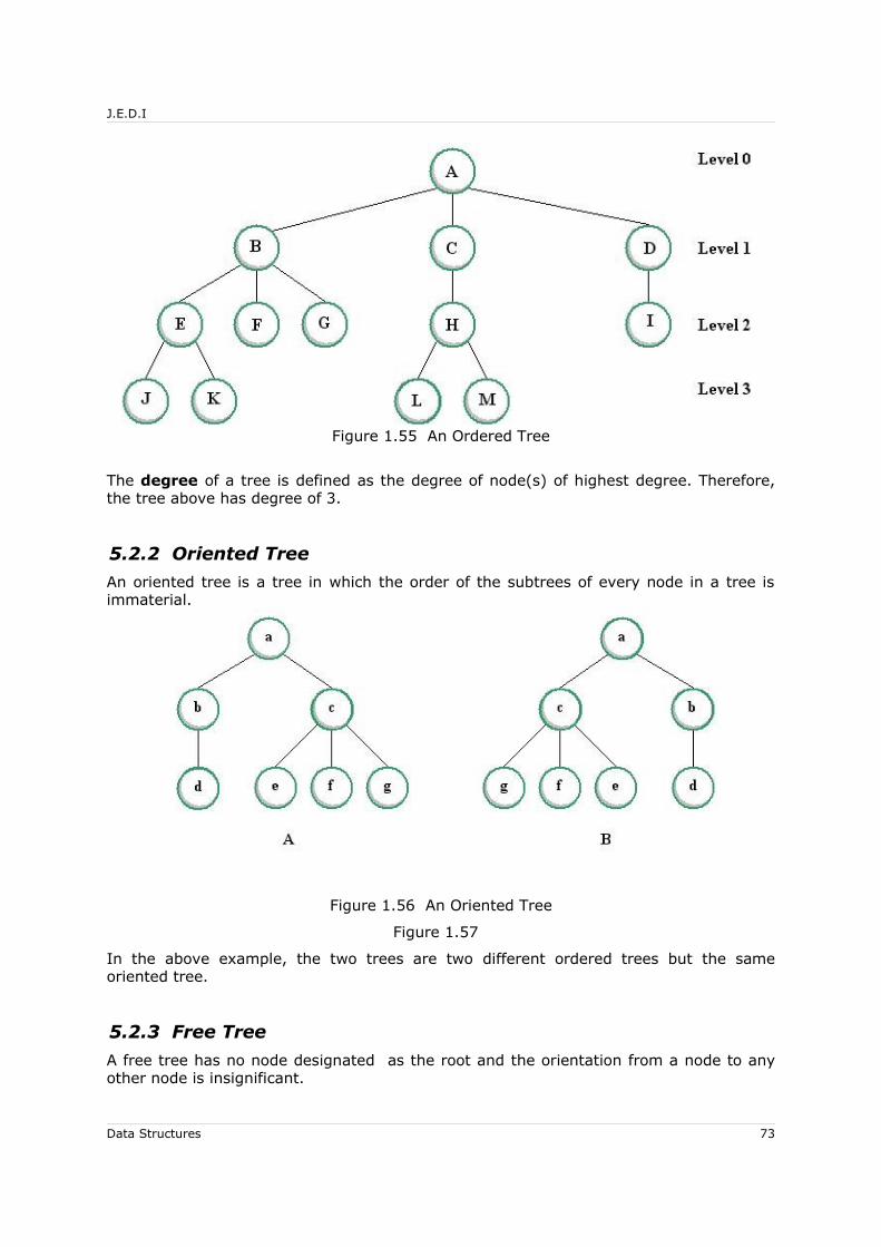
J.E.D.I

Figure 1.55 An Ordered Tree

The degree of a tree is defined as the degree of node(s) of highest degree. Therefore, the tree above has degree of 3.

5.2.2 Oriented Tree

An oriented tree is a tree in which the order of the subtrees of every node in a tree is immaterial.

Figure 1.56 An Oriented Tree

Figure 1.57

In the above example, the two trees are two different ordered trees but the same oriented tree.

5.2.3 Free Tree

A free tree has no node designated as the root and the orientation from a node to any other node is insignificant.

Data Structures 73

J.E.D.I

Figure 1.58 A Free Tree

5.2.4 Progression of Trees

When a free tree is designated a root node, it becomes an oriented tree. When the order of the nodes are defined in an oriented tree, it becomes an ordered tree. The following example illustrates this progression:

Figure 1.59 Progression of Trees

5.3 Link Representation of Trees

Link allocation can be used to represent trees. The figure below shows the structure of the node used in this representation:

Figure 1.60 Node Structure of a Tree Node

Figure 1.61

In the node structure, k is the degree of the tree. SON1, SON2, ..., SONk are links to the k possible sons of a node.

Here are some properties of a tree with n nodes and degree k:• The number of link fields = n * k• The number of non-null links = n-1(#branches)• The number of null links = n*k - (n-1) = n (k-1) + 1

Link representation is the most natural way to represent trees. However, with the above properties, a tree of degree 3 will have 67% of the link space occupied by NULL while with a tree of degree 10, it is 90%! A lot of wasted space is introduced by this approach. If space utilization is a concern, we may opt to use the alternative structure:

Data Structures 74

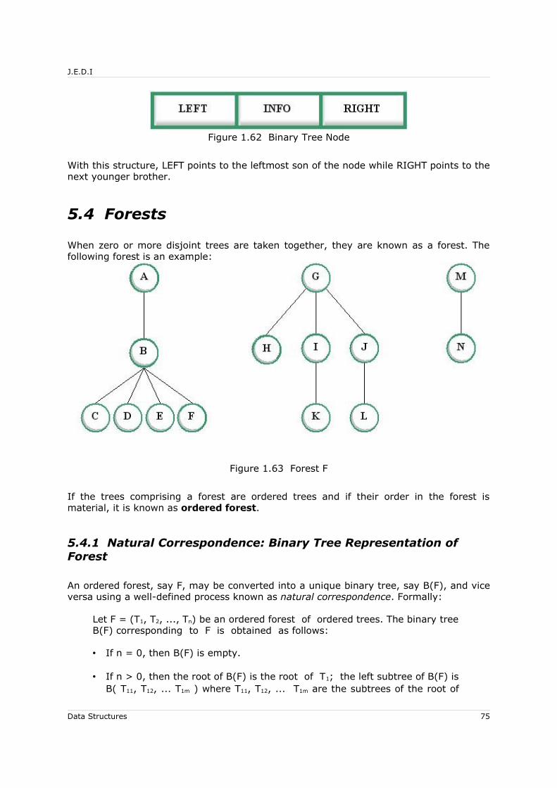
J.E.D.I

Figure 1.62 Binary Tree Node

With this structure, LEFT points to the leftmost son of the node while RIGHT points to the next younger brother.

5.4 Forests

When zero or more disjoint trees are taken together, they are known as a forest. The following forest is an example:

Figure 1.63 Forest F

If the trees comprising a forest are ordered trees and if their order in the forest is material, it is known as ordered forest.

5.4.1 Natural Correspondence: Binary Tree Representation of Forest

An ordered forest, say F, may be converted into a unique binary tree, say B(F), and vice versa using a well-defined process known as natural correspondence. Formally:

Let F = (T1, T2, ..., Tn) be an ordered forest of ordered trees. The binary tree B(F) corresponding to F is obtained as follows:

• If n = 0, then B(F) is empty.

• If n > 0, then the root of B(F) is the root of T1; the left subtree of B(F) is B( T11, T12, ... T1m ) where T11, T12, ... T1m are the subtrees of the root of

Data Structures 75

J.E.D.I

T1; and the right subtree of B(F) is B( T2, T3, ..., Tn ).

Natural correspondence may be implemented using non-recursive approach:

1. Link together the sons in each family from left to right. (Note: the roots of the tree in the forest are brothers, sons of an unknown father.)

2. Remove links from a father to all his sons except the oldest (or leftmost) son.

3. Tilt the resulting figure by 45 degrees.

The following example illustrates the transformation of a forest into its binary tree equivalent:

Data Structures 76

J.E.D.I

Figure 1.64 Example of Natural Correspondence

In natural correspondence, the root is replaced by the root of the first tree, the left subtree is replaced by subtrees of the first tree and the right subtree is replaced by the remaining trees.

5.4.2 Forest Traversal

Just like binary trees, forests can also be traversed. However, since the concept of middle node is not defined, a forest can only be traversed in preorder and postorder.

Data Structures 77

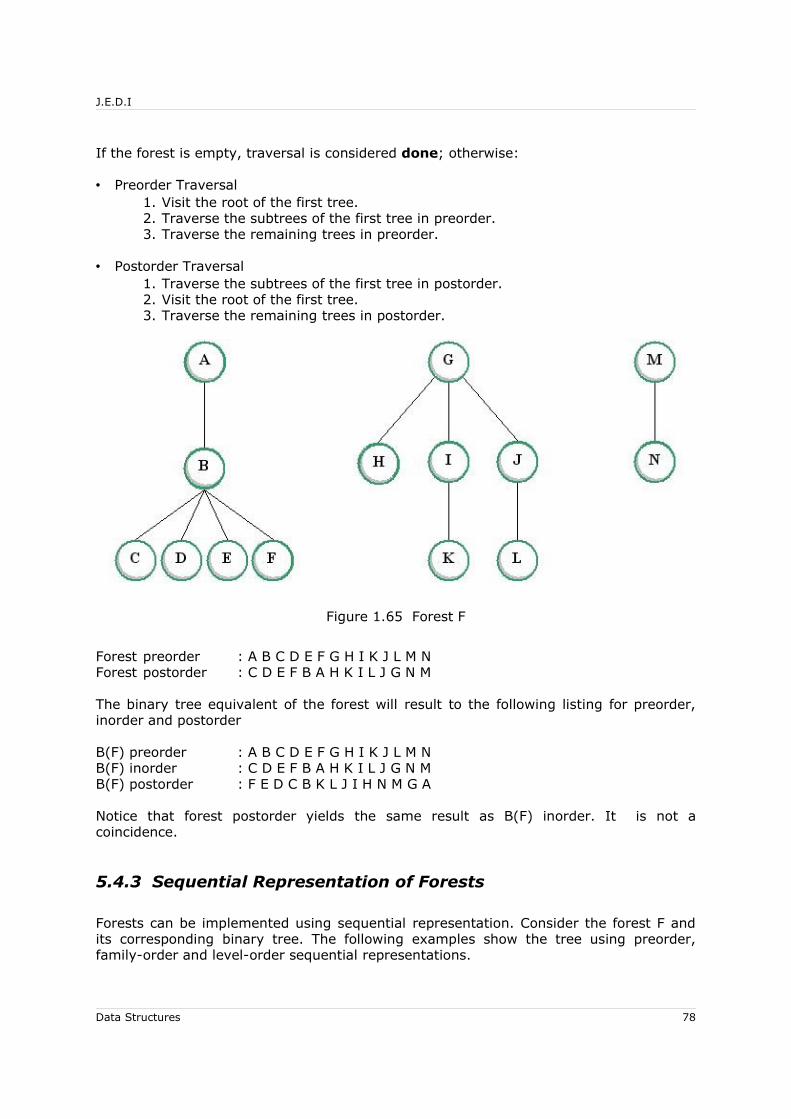
J.E.D.I

If the forest is empty, traversal is considered done; otherwise:

• Preorder Traversal1. Visit the root of the first tree.2. Traverse the subtrees of the first tree in preorder.3. Traverse the remaining trees in preorder.

• Postorder Traversal1. Traverse the subtrees of the first tree in postorder.2. Visit the root of the first tree.3. Traverse the remaining trees in postorder.

Figure 1.65 Forest F

Forest preorder : A B C D E F G H I K J L M NForest postorder : C D E F B A H K I L J G N M

The binary tree equivalent of the forest will result to the following listing for preorder, inorder and postorder

B(F) preorder : A B C D E F G H I K J L M NB(F) inorder : C D E F B A H K I L J G N MB(F) postorder : F E D C B K L J I H N M G A

Notice that forest postorder yields the same result as B(F) inorder. It is not a coincidence.

5.4.3 Sequential Representation of Forests

Forests can be implemented using sequential representation. Consider the forest F and its corresponding binary tree. The following examples show the tree using preorder, family-order and level-order sequential representations.

Data Structures 78

J.E.D.I

5.4.3.1 Preorder Sequential Representation

In this sequential representation, the elements are listed in its preorder sequence and two additional vectors are kept – RLINK and LTAG. RLINK is a pointer from an older to a next younger brother in the forest, or from a father to his right son in its binary tree representation. LTAG is an indicator if a node is terminal (leaf node) and the symbol ')' is used.

The following is the preorder sequential representation of the forest F:

In the implementation, the following is the actual internal representation:

RLINK contains the node pointed to by the current node and LTAG has a value of 1 for every ')' in the representation.

Since a terminal node always immediately precedes a node pointed to by an arrow except the last node in the sequence, the use of data can be lessened by

(1)Eliminating LTAG; or

(2)Replacing RLINK with RTAG that simply identifies the nodes where an arrow emanates

Using the second option will need a stack to establish the relation between nodes since the arrows have the “last in, first out” structure, and using it leads to the following representation:

and this is internally represented as follows:

Data Structures 79

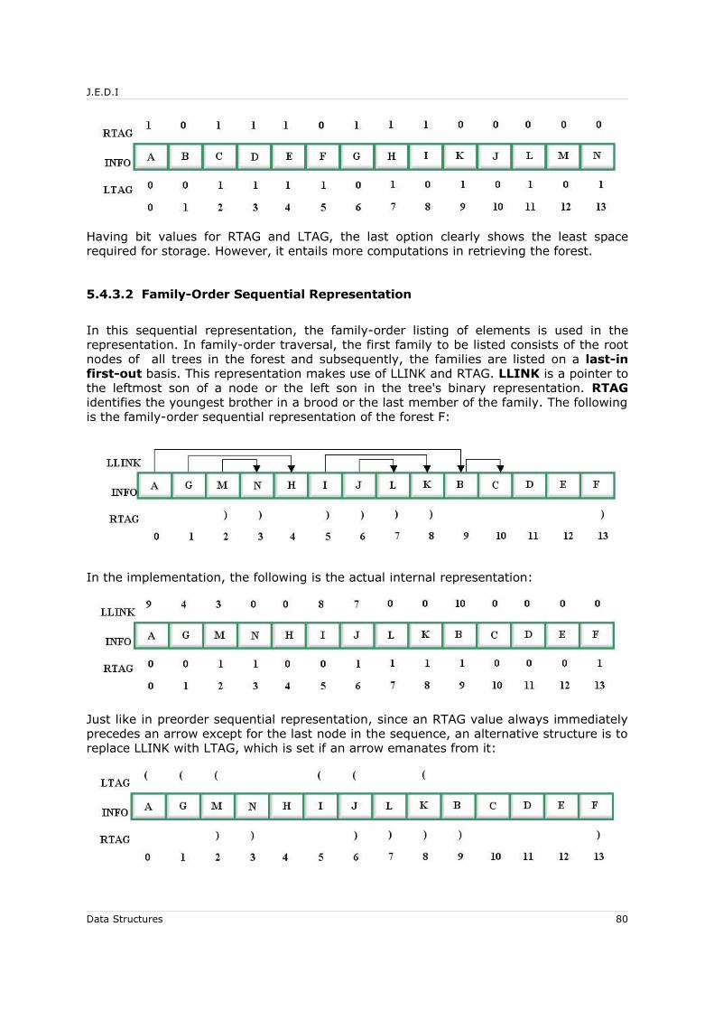
J.E.D.I

Having bit values for RTAG and LTAG, the last option clearly shows the least space required for storage. However, it entails more computations in retrieving the forest.

5.4.3.2 Family-Order Sequential Representation

In this sequential representation, the family-order listing of elements is used in the representation. In family-order traversal, the first family to be listed consists of the root nodes of all trees in the forest and subsequently, the families are listed on a last-in first-out basis. This representation makes use of LLINK and RTAG. LLINK is a pointer to the leftmost son of a node or the left son in the tree's binary representation. RTAG identifies the youngest brother in a brood or the last member of the family. The following is the family-order sequential representation of the forest F:

In the implementation, the following is the actual internal representation:

Just like in preorder sequential representation, since an RTAG value always immediately precedes an arrow except for the last node in the sequence, an alternative structure is to replace LLINK with LTAG, which is set if an arrow emanates from it:

Data Structures 80

J.E.D.I

and internally represented as:

5.4.3.3 Level-Order Sequential Representation

The third option in sequential representation is level-order. In this representation, the forest is traversed in level-order, i.e., top-to-bottom, left-to-right, to obtain the level-order listing of elements. Just like family-order, brothers (which constitute a family) are listed consecutively. LLINK and RTAG are used in the representation. LLINK is a pointer to the oldest son in the forest or the left son in its binary tree representation. RTAG identifies the youngest brother in a brood (or the last member of the family). Using level-order sequential representation, we have the following for the forest F:

Notice that unlike preorder and family-order, arrows cross in this representation. However, it can also be noticed that the first arrow to begin is also the first arrow to end. Having the FIFO (first-in, first-out) structure, queue could be used to establish a relation between nodes. Therefore, just like the previous methods, it could be represented as:

5.4.3.4 Converting from Sequential to Link Representation

Spacewise, sequential representation is good for forests. However, since link representation is more natural for forests, there are instances that we have to use the latter. The following is a method that implements the conversion from sequential to linked representation:

Data Structures 81

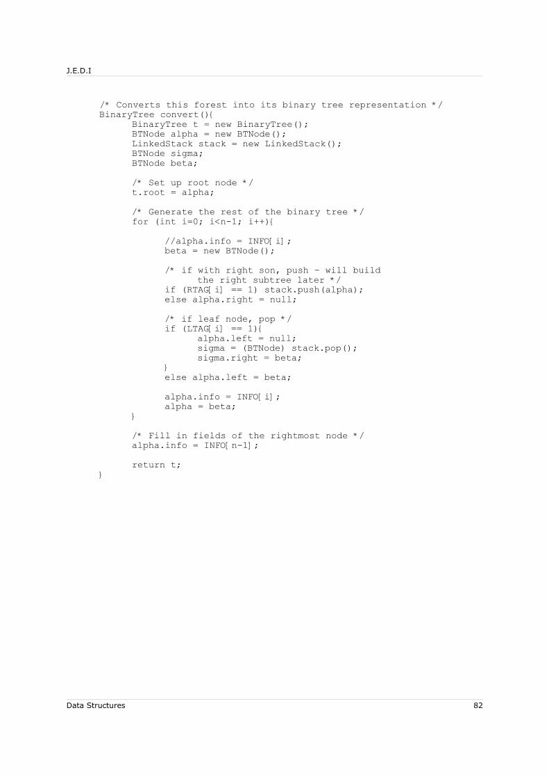
J.E.D.I

/* Converts this forest into its binary tree representation */BinaryTree convert(){

BinaryTree t = new BinaryTree();BTNode alpha = new BTNode();LinkedStack stack = new LinkedStack();BTNode sigma;BTNode beta;/* Set up root node */t.root = alpha;/* Generate the rest of the binary tree */for (int i=0; i<n-1; i++){

//alpha.info = INFO[i];beta = new BTNode();/* if with right son, push – will build

the right subtree later */if (RTAG[i] == 1) stack.push(alpha);else alpha.right = null;/* if leaf node, pop */if (LTAG[i] == 1){

alpha.left = null;sigma = (BTNode) stack.pop();sigma.right = beta;

}else alpha.left = beta;alpha.info = INFO[i];alpha = beta;

}/* Fill in fields of the rightmost node */alpha.info = INFO[n-1];return t;

}

Data Structures 82

J.E.D.I

5.5 Arithmetic Tree Representations

Trees can be represented sequentially using arithmetic tree representation. The tree could be stored sequentially based on the preorder, postorder and level-order listing of its nodes. The degree or the weight of the tree could be stored along with the information. The degree, as defined previously, refers to the number of children a node has while the weight refers to the number of descendants of a node.

Figure 1.66 Ordered Tree T

The following are the different ways to represent the tree above.

5.5.1.1 Preorder Sequence with Degrees

INFO 1 2 5 11 6 12 13 7 3 8 4 9 14 15 16 10DEGREE 3 3 1 0 2 0 0 0 1 0 2 1 2 0 0 0

5.5.1.2 Preorder Sequence with Weights

INFO 1 2 5 11 6 12 13 7 3 8 4 9 14 15 16 10WEIGHT 15 6 1 0 2 0 0 0 1 0 5 3 2 0 0 0

Data Structures 83

J.E.D.I

Postorder Sequence with Degrees

INFO 11 5 12 13 6 7 2 8 3 15 16 14 9 10 4 1DEGREE 0 1 0 0 2 0 3 0 1 0 0 2 1 0 2 3

5.5.1.3 Postorder Sequence with Weights

INFO 11 5 12 13 6 7 2 8 3 15 16 14 9 10 4 1WEIGHT 0 1 0 0 2 0 6 0 1 0 0 2 3 0 5 15

Level-Order Sequence with Degrees

INFO 1 2 3 4 5 6 7 8 9 10 11 12 13 14 15 16DEGREE 3 3 1 2 1 2 0 0 1 0 0 0 0 2 0 0

5.5.1.4 Level-Order Sequence with Weights

INFO 1 2 3 4 5 6 7 8 9 10 11 12 13 14 15 16WEIGHT 15 6 1 5 1 2 0 0 3 0 0 0 0 2 0 0

5.5.2 Application: Trees and the Equivalence Problem

The equivalence problem is another application that makes use of a tree internally represented as an arithmetic tree.

An equivalence relation is a relation between the elements of a set of objects S satisfying the following three properties for any objects x, y and z (not necessarily distinct) in S:

(a) Transitivity: if x ≡ y and y ≡ z then x ≡ z (b) Symmetry: if x ≡ y then y ≡ x (c) Reflexivity: x ≡ x

Examples of equivalence relations are the relation “is equal to” (=) and the “similarity” between binary trees.

5.5.2.1 The Equivalence Problem

Given any pairs of equivalence relations of the form i ≡ j for any i, j in S, determine whether k is equivalent to i, for any k, i in S, on the basis of the given pairs.

To solve the problem we will use the following theorem:

An equivalence relation partitions its set S into disjoint classes, called equivalence classes, such that two elements are equivalent if and only if they belong to the same equivalence class.

Data Structures 84

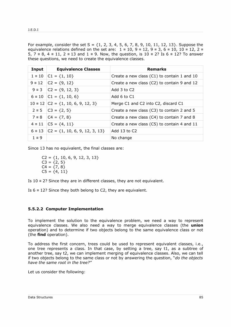
J.E.D.I

For example, consider the set S = {1, 2, 3, 4, 5, 6, 7, 8, 9, 10, 11, 12, 13}. Suppose the equivalence relations defined on the set are: 1 ≡ 10, 9 ≡ 12, 9 ≡ 3, 6 ≡ 10, 10 ≡ 12, 2 ≡ 5, 7 ≡ 8, 4 ≡ 11, 2 ≡ 13 and 1 ≡ 9. Now, the question, is 10 ≡ 2? Is 6 ≡ 12? To answer these questions, we need to create the equivalence classes.

Input Equivalence Classes Remarks

1 ≡ 10 C1 = {1, 10} Create a new class (C1) to contain 1 and 10


9 ≡ 3 C2 = {9, 12, 3} Add 3 to C2

6 ≡ 10 C1 = {1, 10, 6} Add 6 to C1

10 ≡ 12 C2 = {1, 10, 6, 9, 12, 3} Merge C1 and C2 into C2, discard C1




6 ≡ 13 C2 = {1, 10, 6, 9, 12, 3, 13} Add 13 to C2

1 ≡ 9 No change

Since 13 has no equivalent, the final classes are:

C2 = {1, 10, 6, 9, 12, 3, 13}C3 = {2, 5}C4 = {7, 8}C5 = {4, 11}

Is 10 ≡ 2? Since they are in different classes, they are not equivalent.

Is 6 ≡ 12? Since they both belong to C2, they are equivalent.

5.5.2.2 Computer Implementation

To implement the solution to the equivalence problem, we need a way to represent equivalence classes. We also need a way to merge equivalence classes (the union operation) and to determine if two objects belong to the same equivalence class or not (the find operation).

To address the first concern, trees could be used to represent equivalent classes, i.e., one tree represents a class. In that case, by setting a tree, say t1, as a subtree of another tree, say t2, we can implement merging of equivalence classes. Also, we can tell if two objects belong to the same class or not by answering the question, “do the objects have the same root in the tree?”

Let us consider the following:

Data Structures 85

J.E.D.I

Figure 1.67 Merging of Equivalence Classes

Figure 1.68

We are given the equivalence relation i ≡ j where i and j are both roots. To merge the two classes, we set the root of i as a new son of the root of j. This is the merging process, and the subprogram that implements it is what follows:

while (FATHER[i] > 0) {i = FATHER[i];

}while (FATHER[j] > 0) {

j = FATHER[j];}if (i != j) FATHER[j] = k;

The following example shows the graphical illustration of the equivalence problem described above:

Input Forest

1 ≡ 10

1 2 3 4 5 6 7 8 9 10 11 12 13

10 0 0 0 0 0 0 0 0 0 0 0 0

9 ≡ 12

1 2 3 4 5 6 7 8 9 10 11 12 13

10 0 0 0 0 0 0 0 12 0 0 0 0

Data Structures 86

J.E.D.I

Input Forest

9 ≡ 3

1 2 3 4 5 6 7 8 9 10 11 12 13

10 0 0 0 0 0 0 0 12 0 0 3 0

6 ≡ 10

1 2 3 4 5 6 7 8 9 10 11 12 13

10 0 0 0 0 10 0 0 12 0 0 3 0

10 ≡ 12

1 2 3 4 5 6 7 8 9 10 11 12 13

10 0 0 0 0 10 0 0 12 3 0 3 0

2 ≡ 5

1 2 3 4 5 6 7 8 9 10 11 12 13

10 5 0 0 0 10 0 0 12 3 0 3 0

Data Structures 87

J.E.D.I

Input Forest

7 ≡ 8

1 2 3 4 5 6 7 8 9 10 11 12 13

10 5 0 0 0 10 8 0 12 3 0 3 0

4 ≡ 11

1 2 3 4 5 6 7 8 9 10 11 12 13

10 5 0 11 0 10 8 0 12 3 0 3 0

6 ≡ 13

1 2 3 4 5 6 7 8 9 10 11 12 13

10 5 13 11 0 10 8 0 12 3 0 3 0

Data Structures 88

J.E.D.I

1 ≡ 9

1 2 3 4 5 6 7 8 9 10 11 12 13

10 5 13 11 0 10 8 0 12 3 0 3 0

Figure 1.69 An Equivalence Example

The following is the implementation of the algorithm to solve the equivalence problem:

class Equivalence{int[] FATHER;int n;Equivalence(){}Equivalence(int size){

n = size+1; /* +1 since FATHER[0] will not be used */FATHER = new int[n];

}void setSize(int size){

FATHER = new int[size+1];}/* Generates equivalent classes based

on the equivalence pairs j,k */void setEquivalence(int a[], int b[]){

int j, k;for (int i=0; i<a.length; i++){

/* Get the equivalence pair j,k */j = a[i];k = b[i];/* Get the roots of j and k */while (FATHER[j] > 0) j = FATHER[j];while (FATHER[k] > 0) k = FATHER[k];/* If not equivalent, merge the two trees */if (j != k) FATHER[j] = k;

}

Data Structures 89

J.E.D.I

}/* Accepts two elements j and k.

Returns true if equivalent, otherwise returns false */boolean test(int j, int k){

/* Get the roots of j and k */while (FATHER[j] > 0) j = FATHER[j];while (FATHER[k] > 0) k = FATHER[k];/* If they have the same root, they are equivalent */if (j == k) return true;else return false;

}

5.5.2.3 Degeneracy and the Weighting Rule For Union

A problem with the previous algorithm to solve the equivalence problem is degeneracy, i.e., producing a tree that has the deepest possible height, hence making the performance suffer, i.e., time complexity of O(n). To illustrate this, consider the set S = { 1, 2, 3, ..., n } and the equivalence relations 1 ≡ 2, 1 ≡ 3, 1≡ 4, ..., 1 ≡ n. The following figure shows how the tree is constructed:

Figure 1.70 Worst-Case Forest (Tree) in the Equivalence Problem

Now, consider the following tree:

Figure 1.71 Best-Case Forest (Tree) in the Equivalence Problem

Data Structures 90

J.E.D.I

In terms of equivalence classes, the two trees represent the same class. However the second tree requires traversing only one branch from every node to reach the root while it takes n-1 branches for the first tree.

To solve this problem, we will use a technique known as the weighting rule for union. It is defined as follows:

Let node i and node j be roots. If the number of nodes in the tree rooted at node i is greater than the number of nodes in the tree rooted at node j, then make node i the father of node j; else, make node j the father of node i.

In the algorithm, A COUNT vector could be used to count the number of nodes in each tree in the forest. However, if a node is the root of an equivalent class, its entry in the FATHER vector does not matter anymore since a root node has no father. Taking advantage of this, we may use that slot in the FATHER vector instead of using another vector. To distinguish between counts and labels in FATHER, a minus sign is appended to counts. The following method implements the weighting rule for union:

/* Implements the weighting rule for union */void union(int i, int j){

int count = FATHER[i] + FATHER[j];if ( Math.abs(FATHER[i]) > Math.abs(FATHER[j]) ) {

FATHER[j] = i;FATHER[i] = count;

}else{

FATHER[i] = j;FATHER[j] = count;

}}

The UNION operation has time complexity of O(1). If the weighting rule for union is not applied, a sequence of O(n) union-find operations takes, in the worst case, O(n2). Otherwise, if applied, the time complexity is O(n log2n).

Worst-Case Trees

Another observation in using trees for the equivalence problem is related to the worst-case trees generated even when weighting rule for union is applied. Consider the

Data Structures 91

J.E.D.I

following illustration:

Figure 1.72 Worst-Case Trees

The figure shows that the tree grows logarithmically when the weighting rule for union is applied. That is, the worst case trees on n nodes is log2 n. As we have pointed out earlier, a tree having n-1 nodes as children of only one node could be used to represent any equivalence class. In that case, the depth of the worst-case tree could be reduced by applying another technique, and that is the collapsing rule for find. With this, path compression could be done when trying to find the path from the root node to a node p. That is, in the finding process, if the current path is found out not to be optimal, it will be “collapsed” to make it optimal. To illustrate this, consider the following figure:

Figure 1.73 Collapsing Rule for Find 1

Data Structures 92

J.E.D.I

In some relation i ≡ j for any j, it takes at least m steps, i.e., executions of i = FATHER(i), to get to the root.

In the collapsing rule for find, let n1, n2, ..., nm be nodes in the path from node n1 to the root r. To collapse, we make r the father of np, 1 ≤ p < m:

Figure 1.74 Collapsing Rule for Find 2

Figure 1.75

The following method implements this process:

/* Implements the collapsing rule for find.Returns the root of i */

int find(int i){int j, k, l;k = i;

Data Structures 93

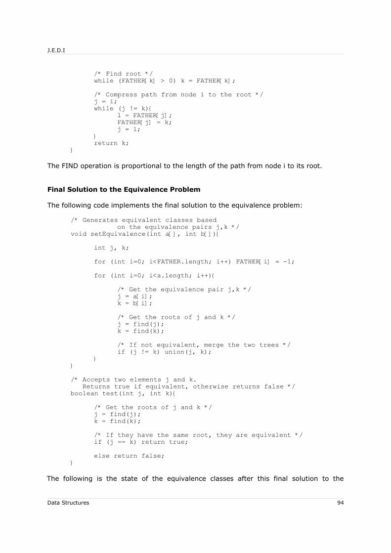
J.E.D.I

/* Find root */while (FATHER[k] > 0) k = FATHER[k];/* Compress path from node i to the root */j = i;while (j != k){

l = FATHER[j];FATHER[j] = k;j = l;

}return k;

}

The FIND operation is proportional to the length of the path from node i to its root.

Final Solution to the Equivalence Problem

The following code implements the final solution to the equivalence problem:

/* Generates equivalent classes basedon the equivalence pairs j,k */

void setEquivalence(int a[], int b[]){int j, k;for (int i=0; i<FATHER.length; i++) FATHER[i] = -1;for (int i=0; i<a.length; i++){

/* Get the equivalence pair j,k */j = a[i];k = b[i];/* Get the roots of j and k */j = find(j);k = find(k);/* If not equivalent, merge the two trees */if (j != k) union(j, k);

}}/* Accepts two elements j and k. Returns true if equivalent, otherwise returns false */boolean test(int j, int k){

/* Get the roots of j and k */j = find(j);k = find(k);/* If they have the same root, they are equivalent */if (j == k) return true;else return false;

}

The following is the state of the equivalence classes after this final solution to the

Data Structures 94

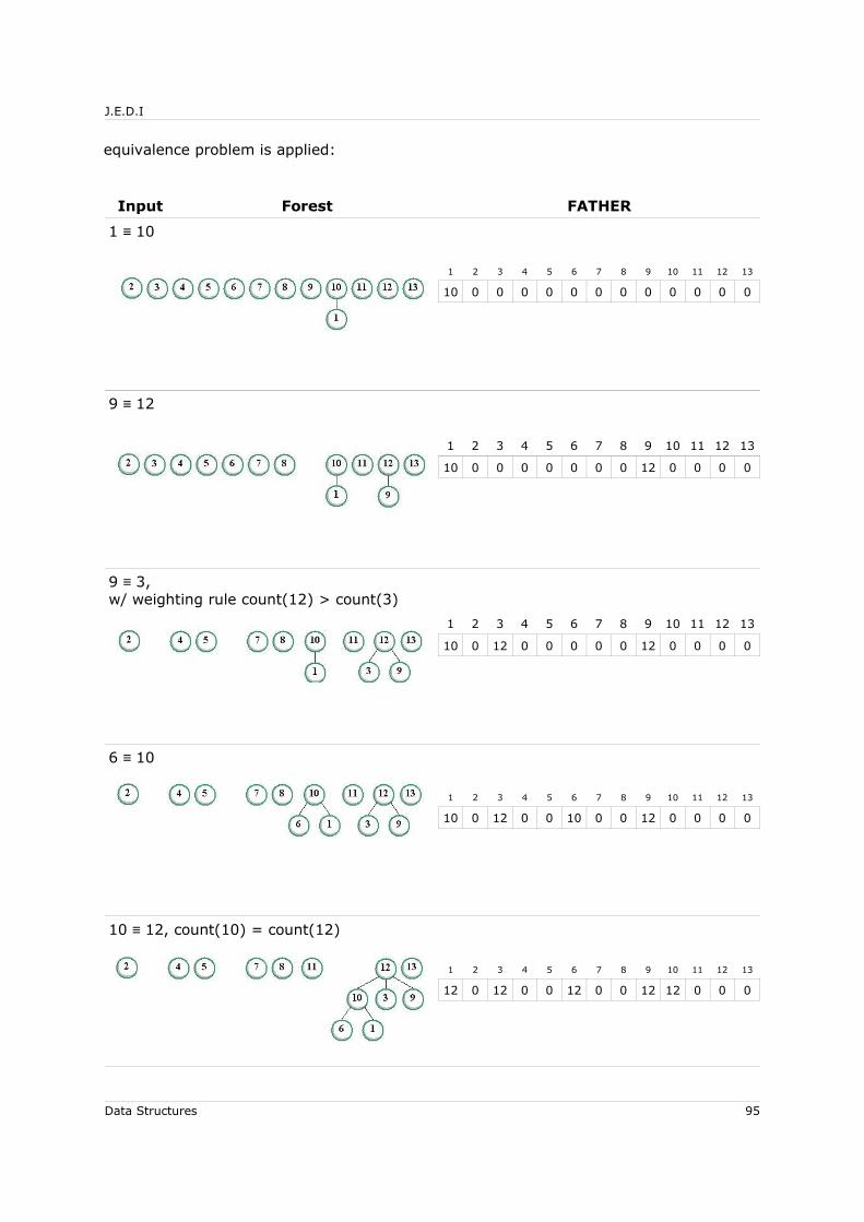
J.E.D.I

equivalence problem is applied:

Input Forest FATHER

1 ≡ 10

1 2 3 4 5 6 7 8 9 10 11 12 13

10 0 0 0 0 0 0 0 0 0 0 0 0

9 ≡ 12

1 2 3 4 5 6 7 8 9 10 11 12 13

10 0 0 0 0 0 0 0 12 0 0 0 0

9 ≡ 3, w/ weighting rule count(12) > count(3)

1 2 3 4 5 6 7 8 9 10 11 12 13

10 0 12 0 0 0 0 0 12 0 0 0 0

6 ≡ 10

1 2 3 4 5 6 7 8 9 10 11 12 13

10 0 12 0 0 10 0 0 12 0 0 0 0

10 ≡ 12, count(10) = count(12)

1 2 3 4 5 6 7 8 9 10 11 12 13

12 0 12 0 0 12 0 0 12 12 0 0 0

Data Structures 95

J.E.D.I

Input Forest FATHER

2 ≡ 5

1 2 3 4 5 6 7 8 9 10 11 12 13

10 5 12 0 0 12 0 0 12 12 0 0 0

7 ≡ 8

1 2 3 4 5 6 7 8 9 10 11 12 13

10 5 12 0 0 12 8 0 12 12 0 0 0

4 ≡ 11

1 2 3 4 5 6 7 8 9 10 11 12 13

12 5 12 11 0 12 8 0 12 12 0 0 0

6 ≡ 13

1 2 3 4 5 6 7 8 9 10 11 12 13

10 5 12 11 0 12 8 0 12 12 0 0 0

1 ≡ 9

1 2 3 4 5 6 7 8 9 10 11 12 13

12 5 12 11 0 12 8 0 12 12 0 0 0

Data Structures 96

J.E.D.I

Figure 1.76 An Example Using Weighted Rule for Union and Collapsing Rule for Find

5.6 Summary

• Trees may be ordered, oriented or free• Link allocation can be used to represent trees. Trees can also be represented

sequentially using arithmetic tree representation.• Zero or more disjoint trees taken together are known as a forest• An ordered forest may be converted into a unique binary tree and vice versa

using natural correspondence• Forests can be traversed in preorder and postorder• Forests can be represented sequentially using preorder, family-order and level-

order sequential representations• The equivalence problem can be solved using trees and the union and find

operations. The weighting rule for union and the collapsing rule for find aid in better algorithm performance.


1. For each of the forests below,

FOREST 1

FOREST 2

Data Structures 97

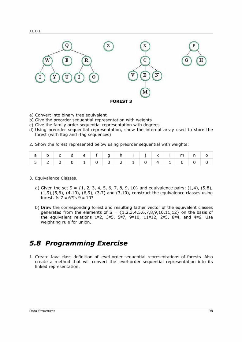
J.E.D.I

FOREST 3

a) Convert into binary tree equivalentb) Give the preorder sequential representation with weightsc) Give the family order sequential representation with degreesd) Using preorder sequential representation, show the internal array used to store the

forest (with ltag and rtag sequences)

2. Show the forest represented below using preorder sequential with weights:

a b c d e f g h i j k l m n o

5 2 0 0 1 0 0 2 1 0 4 1 0 0 0

3. Equivalence Classes.

a) Given the set S = {1, 2, 3, 4, 5, 6, 7, 8, 9, 10} and equivalence pairs: (1,4), (5,8), (1,9),(5,6), (4,10), (6,9), (3,7) and (3,10), construct the equivalence classes using forest. Is 7 ≡ 6?Is 9 ≡ 10?

b) Draw the corresponding forest and resulting father vector of the equivalent classes generated from the elements of S = {1,2,3,4,5,6,7,8,9,10,11,12} on the basis of the equivalent relations 1≡2, 3≡5, 5≡7, 9≡10, 11≡12, 2≡5, 8≡4, and 4≡6. Use weighting rule for union.

5.8 Programming Exercise

1. Create Java class definition of level-order sequential representations of forests. Also create a method that will convert the level-order sequential representation into its linked representation.

Data Structures 98

J.E.D.I

6 Graphs

6.1 Objectives


• Explain the basic concepts and definitions on graphs

• Discuss the methods of graph reprentation: adjacency matrix and adjacency

list

• Traverse graphs using the algorithms depth-first search and breadth-first

search

• Get the minimum cost spanning tree for undirected graphs using Prim's

algorithm and Kruskal's algorithms

• Solve the single-source shortest path problem using Dijkstra's algorithm

• Solve the all-pairs shortest path problem using Floyd's algorithm

6.2 Introduction

This lesson covers the nomenclature for the ADT graph. It also discusses different ways to represent a graph. The two graph traversal algorithms are also covered, as well as the minimum cost spanning tree problem and shortest path problems.


A graph, G = ( V, E ), consists of a finite, non-empty set of vertices (or nodes), V, and a set of edges, E. The following are examples of graph:

Figure 1.77 Examples of Graph

Data Structures 99

J.E.D.I

An undirected graph is a graph in which the pair of vertices representing an edge is unordered, i.e.,( i,j ) and (j,i) represent the same edge.

Figure 1.78 Undirected Graph

Two vertices i and j are adjacent if (i, j) is an edge in E. The edge (i, j) is said to be incident on vertices i and j.

Figure 1.79 Edge (i, j)

Data Structures 100

J.E.D.I

A complete undirected graph is a graph in which an edge connects every pair of vertices. If a complete undirected graph has n vertices, there are n(n -1)/2 edges in it.

Figure 1.80 Complete Undirected Graph

A directed graph or digraph is a graph in which each edge is represented by an ordered pair <i, j>, where i is the head and j is the tail of the edge. The edges <i,j> and <j,i> are two distinct edges.

Figure 1.81 Directed Graph

A complete directed graph is a graph in which every pair of vertices i and j are connected by two edges <i,j> and <j,i>. There are n(n-1) edges in it.

Figure 1.82 Complete Directed Graph

Data Structures 101

J.E.D.I

A subgraph of an undirected (directed) graph G = (V,E) is an undirected (directed)

graph G’ = (V’,E’) such that V ⊆ V and E’ ⊆ E.

Figure 1.83 Examples of Subgraph

Figure 1.84

A path from vertex u to vertex w in an undirected [directed] graph G = (V,E) is a sequence of vertices vo, v1, v2, ..., vm-1, vm where vo ≡ u and vm ≡ w, such that (v0,v1),(v1,v2),..., (vm-1, vm) [ <v0,v1>, <v1,v2>, ..., <vm-1, vm>] are edges in E.

The length of a path refers to the number of edges in it.

A simple path is a path in which all vertices are distinct, except possibly the first and the last.

A simple path is a simple cycle if it has the same start and end vertex.

Two vertices i and j are connected if there is a path from vertex i to vertex j. If for every pair of distinct vertices i and j there is a directed path to and from both vertices, it is said to be strongly connected. A maximal connected subgraph of an undirected graph is known as connected component in an undirected graph. In a directed graph G, strongly connected component refers to the maximal strongly connected component in G.

A weighted graph is a a graph with weights or costs assigned to its edges.

Data Structures 102

J.E.D.I

Figure 1.85 Weighted Graph

Figure 1.86

A spanning tree is a subgraph that connects all the vertices of a graph. The cost of a spanning tree, if it is weighted, is the sum of the weights of the branches (edges) in the spanning tree. A spanning tree that has the minimum cost is referred to as minimum cost spanning tree. This is not necessarily unique for a given graph.

Figure 1.87 Spanning Tree

6.4 Graph Representations

There are several ways to represent a graph, and there are some factors that have to be considered:

• Operations on the graph

• Number of edges relative to the number of vertices in the graph

6.4.1 Adjacency Matrix for Directed Graphs

A directed graph may be represented using a two dimensional matrix, say A, with dimension n x n, where n is the number of vertices. The elements of A are defined as:

A(i,j) =1 if the edge <i,j> exists, 1 ≤ i, j ≤ n = 0 otherwise

The adjacency matrix A can be declared as a boolean matrix if the graph is not weighted. If the graph is weighted, A(i, j) is set to contain the cost of edge <i, j>, but if there is no edge <i, j> in the graph, A(i, j) is set to a very large value. The matrix is then called a cost-adjacency matrix.

For example, the cost-adjacency matrix representation of the following graph is shown below it:

Data Structures 103

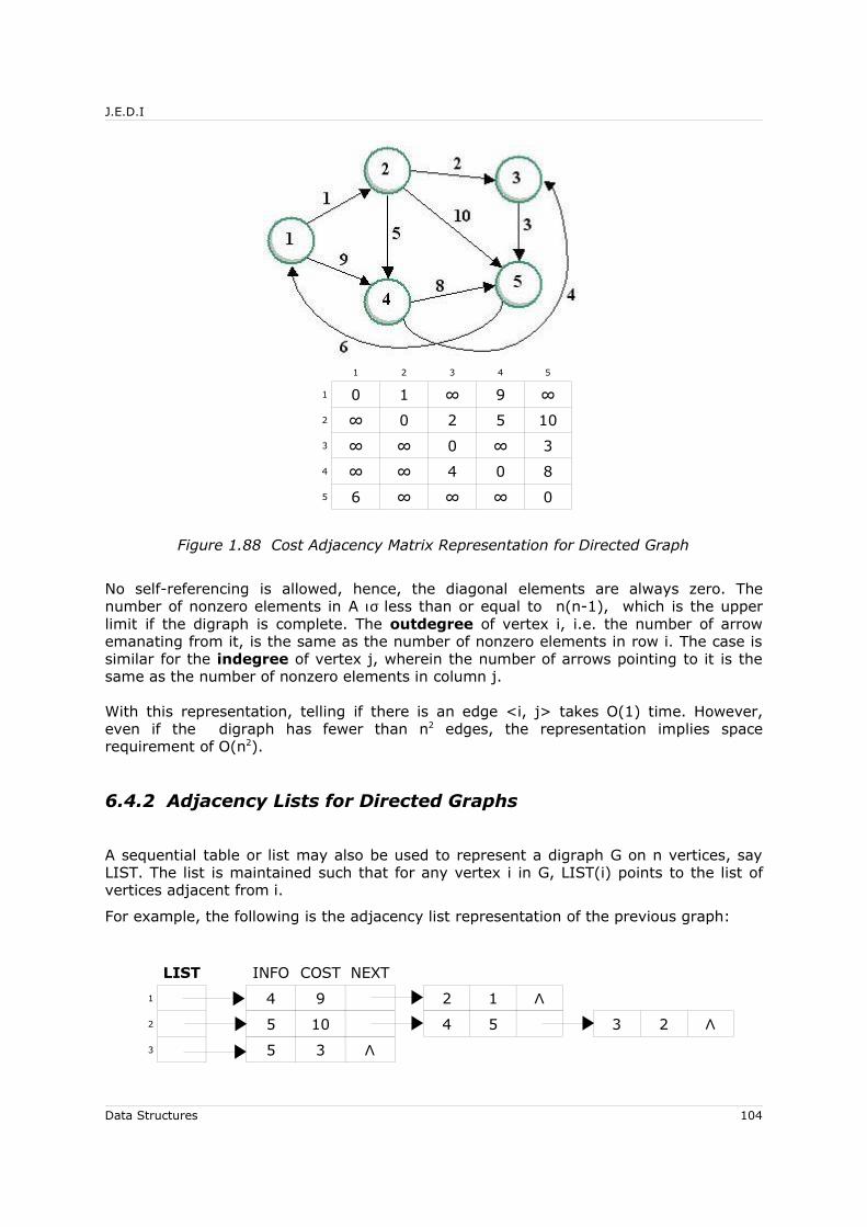
J.E.D.I

1 2 3 4 5

1 0 1 ∞ 9 ∞

2 ∞ 0 2 5 10

3 ∞ ∞ 0 ∞ 3

4 ∞ ∞ 4 0 8

5 6 ∞ ∞ ∞ 0

Figure 1.88 Cost Adjacency Matrix Representation for Directed Graph

No self-referencing is allowed, hence, the diagonal elements are always zero. The number of nonzero elements in A ισ less than or equal to n(n-1), which is the upper limit if the digraph is complete. The outdegree of vertex i, i.e. the number of arrow emanating from it, is the same as the number of nonzero elements in row i. The case is similar for the indegree of vertex j, wherein the number of arrows pointing to it is the same as the number of nonzero elements in column j.

With this representation, telling if there is an edge <i, j> takes O(1) time. However, even if the digraph has fewer than n2 edges, the representation implies space requirement of O(n2).

6.4.2 Adjacency Lists for Directed Graphs

A sequential table or list may also be used to represent a digraph G on n vertices, say LIST. The list is maintained such that for any vertex i in G, LIST(i) points to the list of vertices adjacent from i.

For example, the following is the adjacency list representation of the previous graph:

LIST INFO COST NEXT

1 4 9 2 1 Λ2 5 10 4 5 3 2 Λ3 5 3 Λ

Data Structures 104

J.E.D.I

LIST INFO COST NEXT

4 5 8 3 4 Λ5 1 6 Λ

Figure 1.89 Cost Adjacency List Representation for Directed Graph

6.4.3 Adjacency Matrix for Undirected Graphs

Just like digraph, adjacency matrix may be used to represent undirected graphs. However, they differ in the sense that it is symmetric for undirected graphs, i.e. A(i, j) = A(j, i). It is either the lower or the upper diagonal elements are required to represent the graph. The other part could be regarded as don’t cares (*).

For an undirected graph G on n vertices, the number of nonzero elements in A ≤ n(n-1)/2. The upper limit is attained when G is complete.

For example, the following undirected graph is not weighted. Therefore, its adjacency matrix has bit entries only – A(i,j) = 1 if the edge exists, otherwise 0.

1 2 3 4 5

1 0 * * * *

2 0 0 * * *

3 0 1 0 * *

4 1 0 1 0 *

5 1 1 0 0 0

Figure 1.90 Cost Adjacency Matrix Representation for Undirected Graph

6.4.4 Adjacency List for Undirected Graphs

The representation is similar to adjacency list for directed graph. However, for undirected graph, there is two entries in the list for an edge (i, j).

For example, the adjacency list representation of the previous graph is as follows:

Data Structures 105

J.E.D.I

LIST INFO NEXT

1 5 4 Λ2 5 3 Λ3 4 2 Λ4 3 1 Λ5 2 1 Λ

Figure 1.91 Cost Adjacency List Representation for Undirected Graph

6.5 Graph Traversals

A graph, unlike a tree, has no concept of a root node wherein a traversal method could be started. There is also no natural order among vertices to or from the most recently visited vertex that indicates the one to visit next. In graph traversal, it is also important to note that since a vertex may be adjacent to or from several vertices, there is a possibility to encounter it again. Therefore, there is a need to indicate if a vertex is already visited.

In this section, we will cover two graph traversal algorithms: depth-first search and breadth-first search.

6.5.1 Depth First Search

With depth first search (DFS), the graph is traversed as deeply as possible. Given a graph with vertices marked unvisited, the traversal is performed as follows:

1. Select a start, unvisited vertex. If no vertex can be found, DFS terminates.

2. Mark start vertex visited.

3. Process adjacent vertex:

a) Select an unvisited vertex, say u, adjacent to (or from) the start vertexb) Mark the adjacent vertex visitedc) Initiate a DFS with u as start vertex. If no such vertex can be found, go to

step (1)

4. If more unvisited, adjacent vertices are encountered, go to step (c)

Whenever there is ambiguity on which vertex to visit next in case of several adjacent vertices to the most recently visited one, the vertex with the lower number is chosen to be visited next.

For example, starting at vertex 1, the DFS listing of elements of the following graph is

Data Structures 106

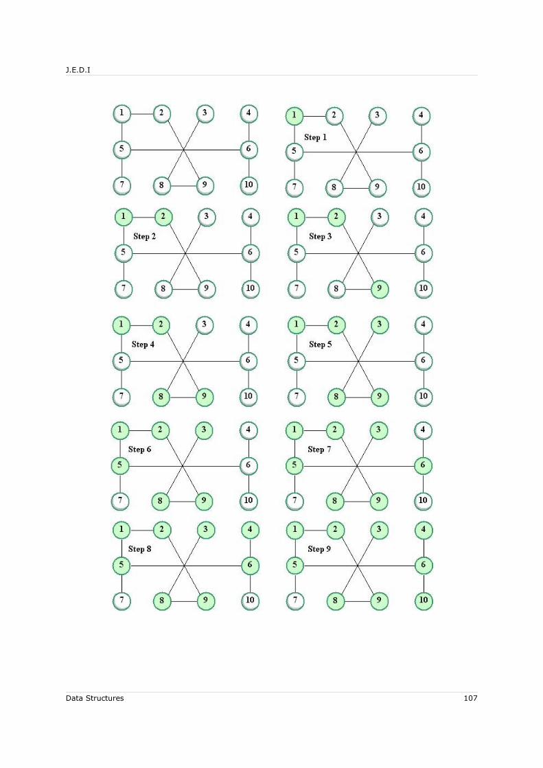
J.E.D.I

Data Structures 107

J.E.D.I

Figure 1.92 Example of Depth First Search

6.5.2 Breadth First Search

Breadth first search (BFS) traverses as broadly as possible. Given a graph with vertices marked unvisited, the traversal is performed as follows:

1. Select an unvisited vertex, say vertex i, and mark it visited. Then, search as broadly as possible from i by visiting all the vertices adjacent to it.

2. Repeat (1) until all the vertices in the graph are visited.

Just like in DFS, conflict on which node to visit next is resolved via visiting in increasing order of numeric label. For example, starting at vertex 1, the BFS listing of elements of the previous graph is

Data Structures 108

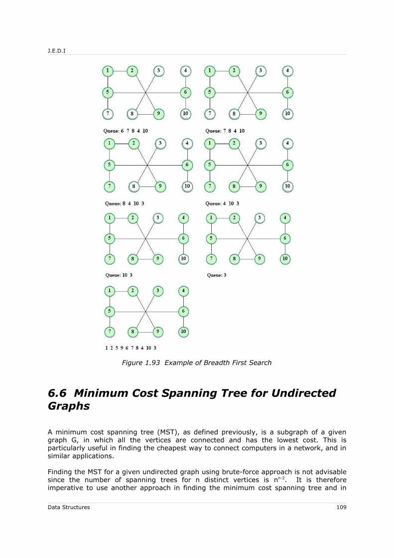
J.E.D.I

Figure 1.93 Example of Breadth First Search

6.6 Minimum Cost Spanning Tree for Undirected Graphs

A minimum cost spanning tree (MST), as defined previously, is a subgraph of a given graph G, in which all the vertices are connected and has the lowest cost. This is particularly useful in finding the cheapest way to connect computers in a network, and in similar applications.

Finding the MST for a given undirected graph using brute-force approach is not advisable since the number of spanning trees for n distinct vertices is nn-2. It is therefore imperative to use another approach in finding the minimum cost spanning tree and in

Data Structures 109

J.E.D.I

this lesson, we will cover algorithms that use the greedy approach. In this approach, a sequence of opportunistic choices succeeds in finding a global optimum. To solve the MST problem, we shall use Prim's and Kruskal's algorithms, which are both greedy algorithms.

6.6.1.1 MST Theorem

Let G = (V,E) be a connected, weighted, undirected graph. Let U be some proper subset of V and (u, v) be an edge of least cost such that u ∈ U and v ∈ (V – U). There exists a minimum cost spanning tree T such that (u, v) is an edge in T.

6.6.1.2 Prim’s Algorithm

This algorithm finds the edge of least cost connecting some vertex u in U to some vertex v in (V – U) at each step of the algorithm:

Let G = (V,E) be a connected, weighted, undirected graph. Let U denote the set of vertices chosen and T denote the set of edges already taken in at any instance of the algorithm.

1. Choose initial vertex from V and place it in U.2. From among the vertices in V - U choose that vertex, say v, which is

connected to some vertex, say u, in U by an edge of least cost. Add vertex v to U and edge (u, v) to T.

3. Repeat (2) until U = V, in which case, T is a minimum cost spanning tree for G.

For example,

Figure 1.94 A Weighted Undirected Graph

having a as the start vertex, the following shows the execution of Prim's algorithm to solve the MST problem:

Data Structures 110

J.E.D.I

Figure 1.95 Result of Applying Prim's Algorithm on Graph in Figure 6.16

6.6.1.3 Kruskal's Algorithm

The other greedy algorithm that is used to find the MST was developed by Kruskal. In this algorithm, the vertices are listed in non-decreasing order of the weights. The first edge to be added to T, which is the MST, is the one that has the lowest cost. An edge is considered if at least one of the vertices is not in the tree found so far.

Now the algorithm:

Let G = (V, E) be a connected, weighted, undirected graph on n vertices. The minimum cost spanning tree, T, is built edge by edge, with the edges considered in non-decreasing order of their cost.

1. Choose the edge with the least cost as the initial edge.

2. The edge of least cost among the remaining edges in E is considered for inclusion in T. If cycle will be created, the edge in T is rejected.

For example,

Data Structures 111

J.E.D.I

The following shows the execution of Kruskal's algorithm in solving the MST problem of the graph above:

Data Structures 112

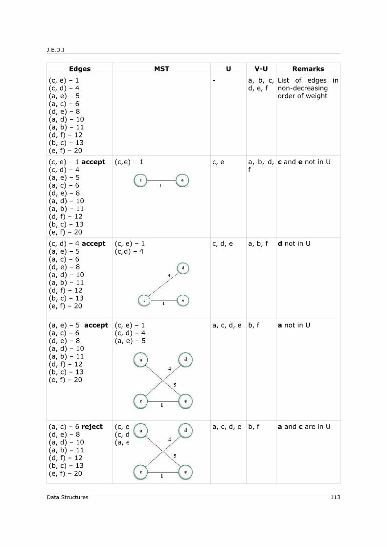
J.E.D.I

Edges MST U V-U Remarks

(c, e) – 1 (c, d) – 4(a, e) – 5(a, c) – 6(d, e) – 8(a, d) – 10(a, b) – 11(d, f) – 12(b, c) – 13(e, f) – 20

- a, b, c, d, e, f

List of edges in non-decreasing order of weight

(c, e) – 1 accept(c, d) – 4(a, e) – 5(a, c) – 6(d, e) – 8(a, d) – 10(a, b) – 11(d, f) – 12(b, c) – 13(e, f) – 20

(c,e) – 1 c, e a, b, d, f

c and e not in U

(c, d) – 4 accept(a, e) – 5(a, c) – 6(d, e) – 8(a, d) – 10(a, b) – 11(d, f) – 12(b, c) – 13(e, f) – 20

(c, e) – 1(c,d) – 4

c, d, e a, b, f d not in U

(a, e) – 5 accept(a, c) – 6(d, e) – 8(a, d) – 10(a, b) – 11(d, f) – 12(b, c) – 13(e, f) – 20

(c, e) – 1(c, d) – 4(a, e) – 5

a, c, d, e b, f a not in U

(a, c) – 6 reject (d, e) – 8(a, d) – 10(a, b) – 11(d, f) – 12(b, c) – 13(e, f) – 20

(c, e) – 1(c, d) – 4(a, e) – 5

a, c, d, e b, f a and c are in U

Data Structures 113

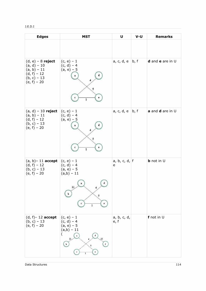
J.E.D.I


(d, e) – 8 reject (a, d) – 10(a, b) – 11(d, f) – 12(b, c) – 13(e, f) – 20

(c, e) – 1(c, d) – 4(a, e) – 5

a, c, d, e b, f d and e are in U

(a, d) – 10 reject(a, b) – 11(d, f) – 12(b, c) – 13(e, f) – 20

(c, e) – 1(c, d) – 4(a, e) – 5

a, c, d, e b, f a and d are in U

(a, b)– 11 accept(d, f) – 12(b, c) – 13(e, f) – 20

(c, e) – 1(c, d) – 4(a, e) – 5(a,b) – 11

a, b, c, d, e

f b not in U

(d, f)– 12 accept(b, c) – 13(e, f) – 20

(c, e) – 1(c, d) – 4(a, e) – 5(a,b) – 11(d,f) – 12

a, b, c, d, e, f

f not in U

Data Structures 114

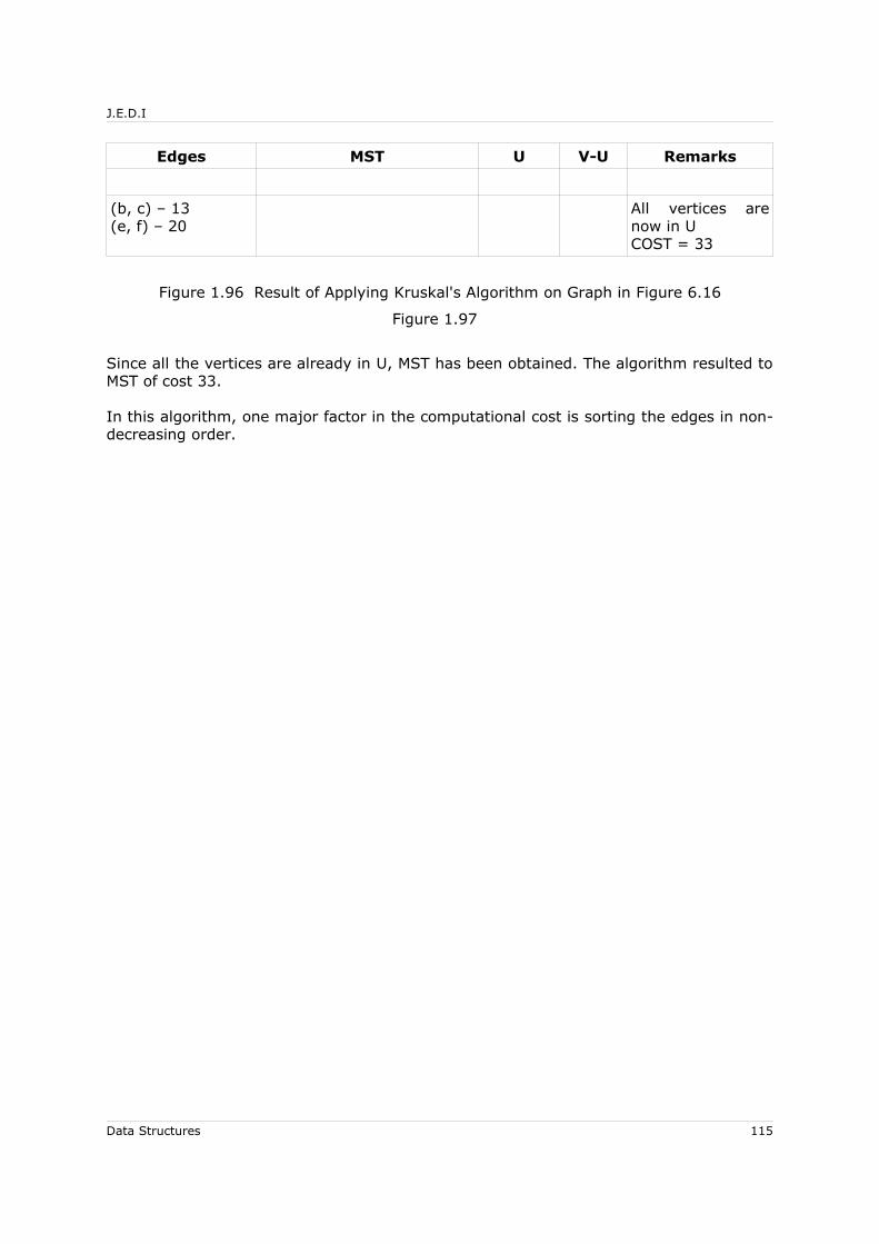
J.E.D.I


(b, c) – 13(e, f) – 20

All vertices are now in UCOST = 33

Figure 1.96 Result of Applying Kruskal's Algorithm on Graph in Figure 6.16

Figure 1.97

Since all the vertices are already in U, MST has been obtained. The algorithm resulted to MST of cost 33.

In this algorithm, one major factor in the computational cost is sorting the edges in non-decreasing order.

Data Structures 115

J.E.D.I

6.7 Shortest Path Problems for Directed Graphs

Another classic set of problems in graphs is finding the shortest path given a weighted graph. In finding the shortest path, there is a need to get the length which, in this case, is the sum of the nonnegative cost of each edge in the path.

There are two path problems on weighted graphs:

• Single Source Shortest Paths (SSSP) Problem that determines the cost of the shortest path from a source vertex u to a destination vertex v, where u and v are elements of V.

• All-Pairs Shortest Paths (APSP) Problem that determines the cost of the shortest path from each vertex to every other vertex in V.

We will discuss the algorithm created by Dijkstra to solve the SSSP problem, and for the APSP, we will use the algorithm developed by Floyd.

6.7.1 Dijkstra's Algorithm for the SSSP Problem

Just like Prim's and Kruskal's, Dijkstra's algorithm uses the greedy approach. In this algorithm, each vertex is assigned a class and a value, where:

• Class 1 vertex is a vertex whose shortest distance from the source vertex, say k, has already been found; Its value is equal to its distance from vertex k along the shortest path.

• Class 2 vertex is a vertex whose shortest distance from k has yet to be found. Its value is its shortest distance from vertex k found thus far.

Let vertex u be the source vertex and vertex v be the destination vertex. Let pivot be the vertex that is most recently considered to be a part of the path. Let path of a vertex be its direct source in the shortest path. Now the algorithm:

1. Place vertex u in class 1 and all other vertices in class 2.2. Set the value of vertex u to zero and the value of all other vertices to

infinity.3. Do the following until vertex v is placed in class 1:

a. Define the pivot vertex as the vertex most recently placed in class 1.

b. Adjust all class 2 nodes in the following way:i. If a vertex is not connected to the pivot vertex, its value

remains the same.ii. If a vertex is connected to the pivot vertex, replace its value by

the minimum of its current value or the value of the pivot vertex plus the distance from the pivot vertex to the vertex in class 2. Set its path to pivot.

c. Choose a class 2 vertex with minimal value and place it in class 1.

Data Structures 116

J.E.D.I

For example, given the following weighted, directed graph, find the shortest path from vertex 1 to vertex 7.

Figure 1.98 A Weighted Directed Graph for SSSP Example

Figure 1.99

Figure 1.100

The following shows the execution of the algorithm:

Vertex class value path Description

1234567

1222222

0∞∞∞∞∞∞

0000000

The source vertex is 1. Its class is set to 1. All others are set to 2. The value of vertex 1 is 0 while the rest are ∞. Path of all vertices are set to 0 since the paths to the vertex from the source have not yet been found.

pivot 1234567

1222222

043∞∞∞∞

0000000

The source vertex is the first pivot. It is connected to vertices 2 and 3. Hence, the values of the vertices are set to 4 and 3 respectively. The class 2 vertex with the minimum value is 3, so it is chosen as the next pivot.

pivot

1234567

1212222

0437∞∞∞

0113000

Class of vertex 3 is set to 1. It is adjacent to vertices 1, 2 and 4 but the value of 1 and 2 are smaller than the value if the path that includes vertex 3 is considered so there will be no change in their values. For vertex 4, the value is set to (value of 3) + cost(3, 4) = 3 + 4 = 7. Path(4) is set to 3.

pivot123

111

043

011

Next pivot is 2. It is adjacent to 4, 5 and 6. Adding the pivot to the current shortest path to 4 will increase its cost, but not with 5 and 6,

Data Structures 117

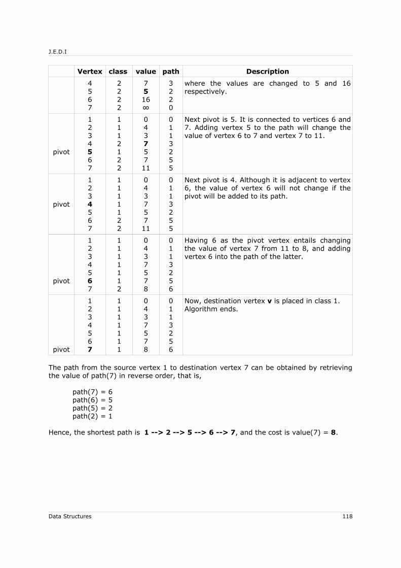
J.E.D.I

Vertex class value path Description

4567

2222

7516∞

3220

where the values are changed to 5 and 16 respectively.

pivot

1234567

1112122

04375711

0113255

Next pivot is 5. It is connected to vertices 6 and 7. Adding vertex 5 to the path will change the value of vertex 6 to 7 and vertex 7 to 11.

pivot

1234567

1111122

04375711

0113255

Next pivot is 4. Although it is adjacent to vertex 6, the value of vertex 6 will not change if the pivot will be added to its path.

pivot

1234567

1111112

0437578

0113256

Having 6 as the pivot vertex entails changing the value of vertex 7 from 11 to 8, and adding vertex 6 into the path of the latter.

pivot

1234567

1111111

0437578

0113256

Now, destination vertex v is placed in class 1. Algorithm ends.

The path from the source vertex 1 to destination vertex 7 can be obtained by retrieving the value of path(7) in reverse order, that is,

path(7) = 6path(6) = 5path(5) = 2path(2) = 1

Hence, the shortest path is 1 --> 2 --> 5 --> 6 --> 7, and the cost is value(7) = 8.

Data Structures 118

J.E.D.I

6.7.2 Floyd's Algorithm for the APSP Problem

In finding all-pairs shortest path, Dijkstra's algorithm may be used with every pair of sources and destinations. However, it is not the best solution there is for the APSP problem. A more elegant approach is to use the algorithm created by Floyd.

The algorithm makes use of cost adjacency matrix representation of a graph. It has a dimension of n x n for n vertices. In this algorithm, let COST be the given adjacency matrix. Let A be the matrix to contain the cost of the shortest path, initially equal to COST. Another n x n matrix, PATH, is needed to contain the immediate vertices along the shortest path:

PATH (i,j) = 0 initially, indicates that the shortest path between i and j is the edge (i,j) if it exists

= k if, including k in the path from i to j at the kth iteration, yields a shorter path

The algorithm is as follows:

1. Initialize A to be equal to COST:

A(i, j) = COST(i, j), 1 ≤ i, j ≤ n

2. If the cost of passing through the intermediate vertex k from vertex i to vertex j will cost less than direct access from i to j, replace A(i,j) with this cost and update PATH(i,j) as well:

For k = 1, 2, 3, ..., n

a) A(i, j) = minimum [ Ak-1(i, j), Ak-1(i, k) + Ak-1(k, j) ] , 1 ≤ i, j ≤ n

b) If ( A(i, j) == Ak-1(i, k) + Ak-1(k, j) ) set PATH(i, j) = k

For example, solve the APSP problem on the following graph using Floyd's algorithm:

Figure 1.101 A Weighted Directed Graph for APSP Example

Figure 1.102

Since no self-referencing is allowed, there is no need to compute for A(j, j), for 1≤j≤n.

Data Structures 119

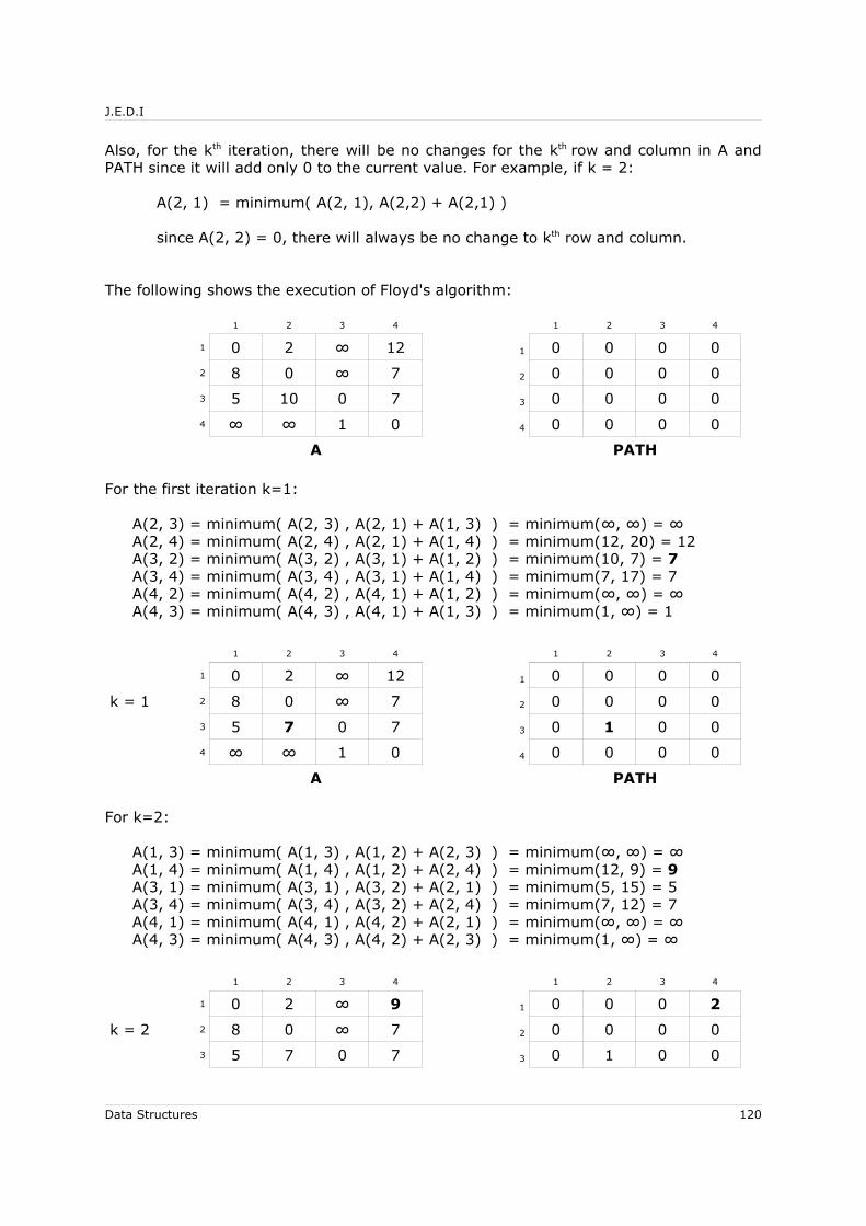
J.E.D.I

Also, for the kth iteration, there will be no changes for the kth row and column in A and PATH since it will add only 0 to the current value. For example, if k = 2:

A(2, 1) = minimum( A(2, 1), A(2,2) + A(2,1) )

since A(2, 2) = 0, there will always be no change to kth row and column.

The following shows the execution of Floyd's algorithm:

1 2 3 4 1 2 3 4

1 0 2 ∞ 12 1 0 0 0 0

2 8 0 ∞ 7 2 0 0 0 0

3 5 10 0 7 3 0 0 0 0

4 ∞ ∞ 1 0 4 0 0 0 0

A PATH

For the first iteration k=1:

A(2, 3) = minimum( A(2, 3) , A(2, 1) + A(1, 3) ) = minimum(∞, ∞) = ∞A(2, 4) = minimum( A(2, 4) , A(2, 1) + A(1, 4) ) = minimum(12, 20) = 12A(3, 2) = minimum( A(3, 2) , A(3, 1) + A(1, 2) ) = minimum(10, 7) = 7A(3, 4) = minimum( A(3, 4) , A(3, 1) + A(1, 4) ) = minimum(7, 17) = 7A(4, 2) = minimum( A(4, 2) , A(4, 1) + A(1, 2) ) = minimum(∞, ∞) = ∞ A(4, 3) = minimum( A(4, 3) , A(4, 1) + A(1, 3) ) = minimum(1, ∞) = 1

1 2 3 4 1 2 3 4

1 0 2 ∞ 12 1 0 0 0 0

k = 1 2 8 0 ∞ 7 2 0 0 0 0

3 5 7 0 7 3 0 1 0 0

4 ∞ ∞ 1 0 4 0 0 0 0

A PATH

For k=2:

A(1, 3) = minimum( A(1, 3) , A(1, 2) + A(2, 3) ) = minimum(∞, ∞) = ∞A(1, 4) = minimum( A(1, 4) , A(1, 2) + A(2, 4) ) = minimum(12, 9) = 9A(3, 1) = minimum( A(3, 1) , A(3, 2) + A(2, 1) ) = minimum(5, 15) = 5A(3, 4) = minimum( A(3, 4) , A(3, 2) + A(2, 4) ) = minimum(7, 12) = 7A(4, 1) = minimum( A(4, 1) , A(4, 2) + A(2, 1) ) = minimum(∞, ∞) = ∞A(4, 3) = minimum( A(4, 3) , A(4, 2) + A(2, 3) ) = minimum(1, ∞) = ∞

1 2 3 4 1 2 3 4

1 0 2 ∞ 9 1 0 0 0 2

k = 2 2 8 0 ∞ 7 2 0 0 0 0

3 5 7 0 7 3 0 1 0 0

Data Structures 120

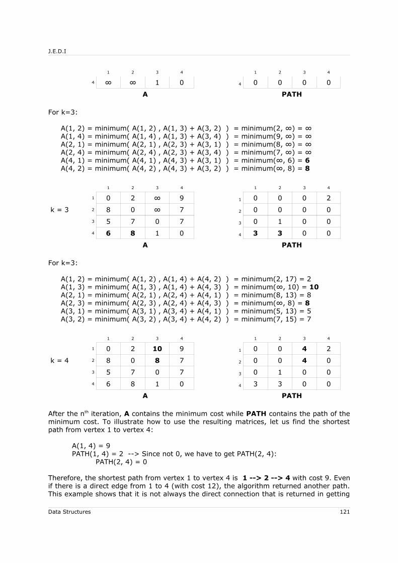
J.E.D.I

1 2 3 4 1 2 3 4

4 ∞ ∞ 1 0 4 0 0 0 0

A PATH

For k=3:

A(1, 2) = minimum( A(1, 2) , A(1, 3) + A(3, 2) ) = minimum(2, ∞) = ∞A(1, 4) = minimum( A(1, 4) , A(1, 3) + A(3, 4) ) = minimum(9, ∞) = ∞A(2, 1) = minimum( A(2, 1) , A(2, 3) + A(3, 1) ) = minimum(8, ∞) = ∞A(2, 4) = minimum( A(2, 4) , A(2, 3) + A(3, 4) ) = minimum(7, ∞) = ∞A(4, 1) = minimum( A(4, 1) , A(4, 3) + A(3, 1) ) = minimum(∞, 6) = 6A(4, 2) = minimum( A(4, 2) , A(4, 3) + A(3, 2) ) = minimum(∞, 8) = 8

1 2 3 4 1 2 3 4

1 0 2 ∞ 9 1 0 0 0 2

k = 3 2 8 0 ∞ 7 2 0 0 0 0

3 5 7 0 7 3 0 1 0 0

4 6 8 1 0 4 3 3 0 0

A PATH

For k=3:

A(1, 2) = minimum( A(1, 2) , A(1, 4) + A(4, 2) ) = minimum(2, 17) = 2A(1, 3) = minimum( A(1, 3) , A(1, 4) + A(4, 3) ) = minimum(∞, 10) = 10A(2, 1) = minimum( A(2, 1) , A(2, 4) + A(4, 1) ) = minimum(8, 13) = 8A(2, 3) = minimum( A(2, 3) , A(2, 4) + A(4, 3) ) = minimum(∞, 8) = 8A(3, 1) = minimum( A(3, 1) , A(3, 4) + A(4, 1) ) = minimum(5, 13) = 5A(3, 2) = minimum( A(3, 2) , A(3, 4) + A(4, 2) ) = minimum(7, 15) = 7

1 2 3 4 1 2 3 4

1 0 2 10 9 1 0 0 4 2

k = 4 2 8 0 8 7 2 0 0 4 0

3 5 7 0 7 3 0 1 0 0

4 6 8 1 0 4 3 3 0 0

A PATH

After the nth iteration, A contains the minimum cost while PATH contains the path of the minimum cost. To illustrate how to use the resulting matrices, let us find the shortest path from vertex 1 to vertex 4:

A(1, 4) = 9 PATH(1, 4) = 2 --> Since not 0, we have to get PATH(2, 4):

PATH(2, 4) = 0

Therefore, the shortest path from vertex 1 to vertex 4 is 1 --> 2 --> 4 with cost 9. Even if there is a direct edge from 1 to 4 (with cost 12), the algorithm returned another path. This example shows that it is not always the direct connection that is returned in getting

Data Structures 121

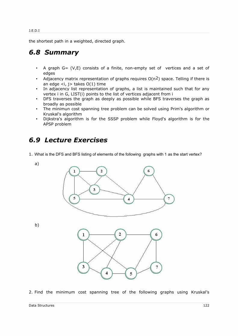
J.E.D.I

the shortest path in a weighted, directed graph.

6.8 Summary

• A graph G= (V,E) consists of a finite, non-empty set of vertices and a set of edges

• Adjacency matrix representation of graphs requires O(n2) space. Telling if there is an edge <i, j> takes O(1) time

• In adjacency list representation of graphs, a list is maintained such that for any vertex i in G, LIST(i) points to the list of vertices adjacent from i

• DFS traverses the graph as deeply as possible while BFS traverses the graph as broadly as possible

• The minimun cost spanning tree problem can be solved using Prim's algorithm or Kruskal's algorithm

• Dijkstra's algorithm is for the SSSP problem while Floyd's algorithm is for the APSP problem


1. What is the DFS and BFS listing of elements of the following graphs with 1 as the start vertex?

a)

b)

2. Find the minimum cost spanning tree of the following graphs using Kruskal’s

Data Structures 122

J.E.D.I

algorithm and Prim’s algorithm. Give the cost of the MST.

a)

b)

3. Solve for the SSSP problem of the following graphs using Dijkstra's algorithm. Show the value, class and path of the vertices for each iteration:

a)

DIJKSTRA 1 (Source: 8, Destination: 4)

Data Structures 123

J.E.D.I

b)

DIJKSTRA 2 (Source: 1, Destination: 7)

4. Solve the APSP of the following graphs by giving the matrices A and Path using Floyd's algorithm:


1. Create a Java class definition for weighted directed graphs using adjacency matrix representation.

2. Implement the two graph traversal algorithms.

3. Shortest Path Using Dijkstra’s Algorithm.

Implement a shortest path adviser given a map and cost of each connection. The program shall ask for an input file containing the sources or destinations (vertices) and the connections between the locations (edges) along with the cost. The locations are of the form (number, location) where number is an integer assigned to a vertex and location is the name of the vertex. Every (number, location) pair must be placed on a separate line in the input file. To terminate the input, use (0, 0). Connections shall be retrieved also from the same file. An edge definition must be of the form (i, j, k), one line per edge, where i is the number assigned to the source, j the number assigned to the destination and k the cost of reaching j from i (Remember, we use directed graphs here). Terminate the input using (0, 0, 0).

After the input, create a map and show it to the user. Ask the user for the source and destination and give the shortest path by using Dijkstra’s algorithm.

Data Structures 124

J.E.D.I

Show the output on the screen. The output consists of the path and its cost. The path must be of the form:

source location 2 … location n-1 destination

Sample Input File

(1, Math Building)(2, Science Building)(3, Engineering)..(0, 0)(1, 2, 10)(1, 3, 5)(3, 2, 2)..(0, 0, 0)

start of edge definition

Sample Program Flow

[ MAP and LEGEND ]

Input Source: 1Input Destination: 2

Source: Math BuildingDestination: Science Building

Path: Math Building Engineering Science BuildingCost: 7

Data Structures 125

J.E.D.I

7 Lists

7.1 Objectives


• Explain the basic conceps and definitions on lists

• Use the different list representations: sequential and linked

• Differentiate singly-linked list, doubly-linked list, circular list and list with

header nodes

• Explain how list is applied in polynomial arithmetic

• Discuss the data structures used in dynamic memory allocation using

sequential-fit methods and buddy-system methods

7.2 Introduction

List is a data structure that is based on sequences of items. In this lesson, we will cover the two types of lists - linear and generalized lists - and their different representations. Singly-linked, circular and doubly-linked lists will also be explored. Moreover, two applications shall be covered – polynomial arithmetic and dynamic memory allocation. Polynomial arithmetic includes representation of polynomials and arithmetic operations defined on them. Dynamic memory allocation covers pointers and allocation strategies. There will also be a short discussion on the concepts of fragmentation.

7.3 Definition and Related Concepts

List is a finite set of zero or more elements. The elements of a list may be atoms or lists. An atom is assumed to be distinguishable from a list. Lists are classified into two types – linear and generalized. Linear list contains atom elements only, and are sequentially ordered. Generalized list could contain both list and atom elements.

7.3.1 Linear List

Linear ordering of atoms is the essential property of linear list. The following is the notation for this type of list:

L = ( i1, i2, i3, ..., in )

Several operations could be done with a linear list. Insertion may be done at any

Data Structures 126

J.E.D.I

position. Similarly, any element may be deleted from any position. The following are the operations that can be done on linear lists:

• Initializing (setting the list to NULL)

• Determining if a list is empty (checking if L != NULL)

• Finding the length (getting the number of elements)

• Accessing the ith element, 0 ≤ i ≤ n-1

• Updating the ith element

• Deleting the ith element

• Inserting a new element

• Combining two or more lists into a single list

• Splitting a list into two or more lists

• Duplicating a list

• Erasing a list

• Searching for a value

• Sorting the list

7.3.2 Generalized List

Generalized list could contain list and atom elements. It has depth and length. Generalized list is also known as list structure, or simply list. The following is an example:

L = ((a, b, ( c, ( ))), d, ( ), ( e,( ), (f, (g, (a))), d ))

Data Structures 127

J.E.D.I

Figure 1.103 A Generalized List

Figure 1.104

In the example, list L has four elements. The first element is the list ( a, b, (c, ( ) )), the second is the atom d, the third is the null set () and the fourth is the list ( e, ( ), (f, (g, (a))), d).

7.4 List Representations

A way to represent a list is to organize the elements one after another in a sequential structure like an array. Another way to implement it is to chain nodes containing the elements of the list using linked representation.

7.4.1 Sequential Representation of Singly-Linked Linear List

In sequential representation, the elements are stored contiguously. There is a pointer to the last item in the list. The following shows a list using sequential representation:

Figure 1.105 Sequential Representation of List

With this representation, it would take O(1) time to access and update the i th element in the list. By keeping track of the last item, it would take O(1) time to tell if the list is empty and to find the length of the list. It has a condition, though, that the first element should always be stored at the first index L(0). In that case, insertion and deletion would require shifting of elements to ensure that the list satisfies this condition. In the worst case, this would entail shifting all the elements in the array, resulting to time complexity of O(n) for insertion and deletion, for n elements. In combining two lists, a larger array is required if the combined size will not fit in any of the two lists. That would entail copying all the elements of the two lists into the new list. Duplicating a list would require traversing the entire list, hence, a time complexity of O(n). Searching for a particular value would take O(1) time if the element is the first one in the list; however, worst case is when it is the last, where traversal of the entire list would be necessary. In such a case, the time complexity is O(n).

Sequential allocation, being static in nature, is a disadvantage for lists with unpredictable size, i.e., the size is not known at the time of initialization, and with a lot of insertions and deletions, would eventually need to grow or shrink. Copying the overflowed list into a larger array and discarding the old one would do, but it would be a waste of time. In such cases, it would be better to use linked representation.

Data Structures 128

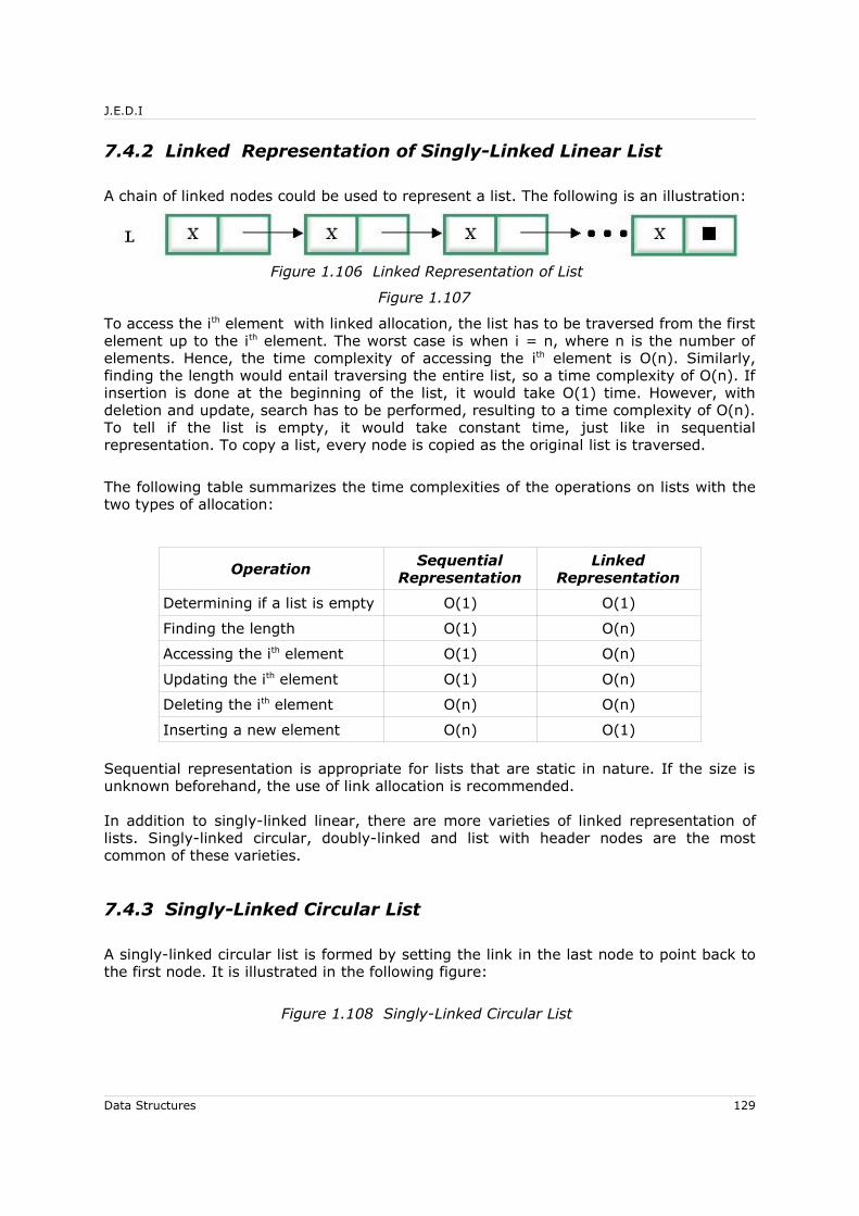
J.E.D.I

7.4.2 Linked Representation of Singly-Linked Linear List

A chain of linked nodes could be used to represent a list. The following is an illustration:

Figure 1.106 Linked Representation of List

Figure 1.107

To access the ith element with linked allocation, the list has to be traversed from the first element up to the ith element. The worst case is when i = n, where n is the number of elements. Hence, the time complexity of accessing the ith element is O(n). Similarly, finding the length would entail traversing the entire list, so a time complexity of O(n). If insertion is done at the beginning of the list, it would take O(1) time. However, with deletion and update, search has to be performed, resulting to a time complexity of O(n). To tell if the list is empty, it would take constant time, just like in sequential representation. To copy a list, every node is copied as the original list is traversed.

The following table summarizes the time complexities of the operations on lists with the two types of allocation:

Operation Sequential Representation

Linked Representation

Determining if a list is empty O(1) O(1)

Finding the length O(1) O(n)

Accessing the ith element O(1) O(n)

Updating the ith element O(1) O(n)

Deleting the ith element O(n) O(n)

Inserting a new element O(n) O(1)

Sequential representation is appropriate for lists that are static in nature. If the size is unknown beforehand, the use of link allocation is recommended.

In addition to singly-linked linear, there are more varieties of linked representation of lists. Singly-linked circular, doubly-linked and list with header nodes are the most common of these varieties.

7.4.3 Singly-Linked Circular List

A singly-linked circular list is formed by setting the link in the last node to point back to the first node. It is illustrated in the following figure:

Figure 1.108 Singly-Linked Circular List

Data Structures 129

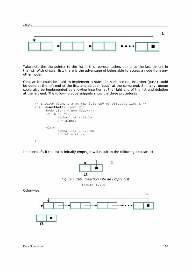
J.E.D.I

Take note the the pointer to the list in this representation, points at the last elment in the list. With circular list, there is the advantage of being able to access a node from any other node.

Circular list could be used to implement a stack. In such a case, insertion (push) could be done at the left end of the list, and deletion (pop) at the same end. Similarly, queue could also be implemented by allowing insertion at the right end of the list and deletion at the left end. The following code snippets show the three procedures:

/* Inserts element x at the left end of circular list L */void insertLeft(Object x){

Node alpha = new Node(x);if (L == null){

alpha.link = alpha;L = alpha;

}else{

alpha.link = L.link;L.link = alpha;

}}

In insertLeft, if the list is initially empty, it will result to the following circular list:

Figure 1.109 Insertion into an Empty List

Figure 1.110

Otherwise,

Data Structures 130

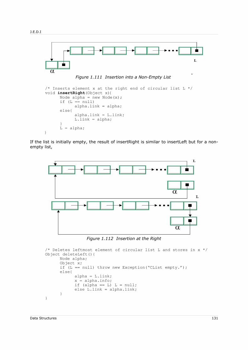
J.E.D.I

Figure 1.111 Insertion into a Non-Empty List

/* Inserts element x at the right end of circular list L */void insertRight(Object x){

Node alpha = new Node(x);if (L == null)

alpha.link = alpha;else{

alpha.link = L.link;L.link = alpha;

}L = alpha;

}

If the list is initially empty, the result of insertRight is similar to insertLeft but for a non-empty list,

Figure 1.112 Insertion at the Right

/* Deletes leftmost element of circular list L and stores in x */Object deleteLeft(){

Node alpha;Object x;if (L == null) throw new Exception(“CList empty.”);else{

alpha = L.link;x = alpha.info;if (alpha == L) L = null;else L.link = alpha.link;

}}

Data Structures 131

J.E.D.I

Performing deleteLeft on a non-empty list is illustated below:

Figure 1.113 Delete from Left

All these three procedures have O(1) time complexity.

Another operation that takes O(1) time in circular lists is concatenation. That is, given two lists

L1 = (a1, a2, ..., am) and

L2 = (b1, b2, ..., bn)

where m, n is ≥ 0, the resulting lists are

L1 = (a1, a2, ..., am, b1, b2, ..., bn)

L2 = null

This could be done by simple manipulations of the pointer field of the nodes:

/* Concatenate list L2 to this list (L) */void concatenate(L2){

if (L2 != null)if (L != null){

Node alpha = L.link;L.link = L2.link;L2.link = alpha;

}}

If L2 is non-empty, the process of concatenation is illustrated below:

Data Structures 132

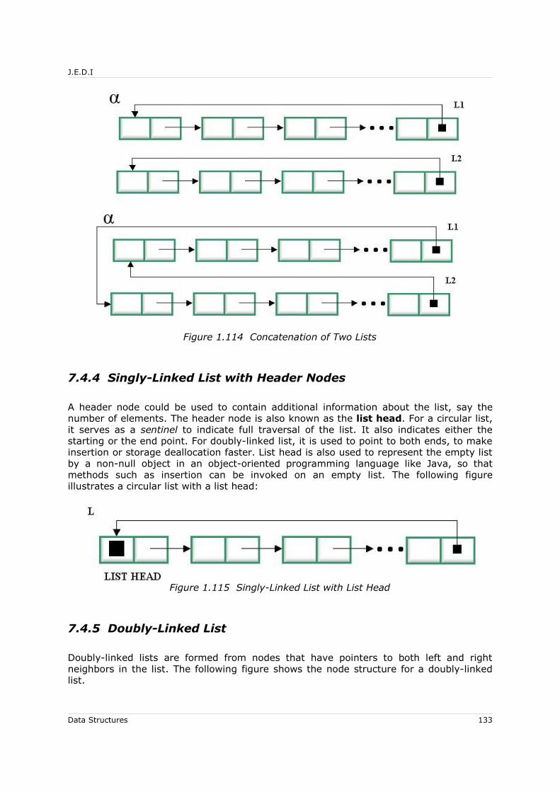
J.E.D.I

Figure 1.114 Concatenation of Two Lists

7.4.4 Singly-Linked List with Header Nodes

A header node could be used to contain additional information about the list, say the number of elements. The header node is also known as the list head. For a circular list, it serves as a sentinel to indicate full traversal of the list. It also indicates either the starting or the end point. For doubly-linked list, it is used to point to both ends, to make insertion or storage deallocation faster. List head is also used to represent the empty list by a non-null object in an object-oriented programming language like Java, so that methods such as insertion can be invoked on an empty list. The following figure illustrates a circular list with a list head:

Figure 1.115 Singly-Linked List with List Head

7.4.5 Doubly-Linked List

Doubly-linked lists are formed from nodes that have pointers to both left and right neighbors in the list. The following figure shows the node structure for a doubly-linked list.

Data Structures 133

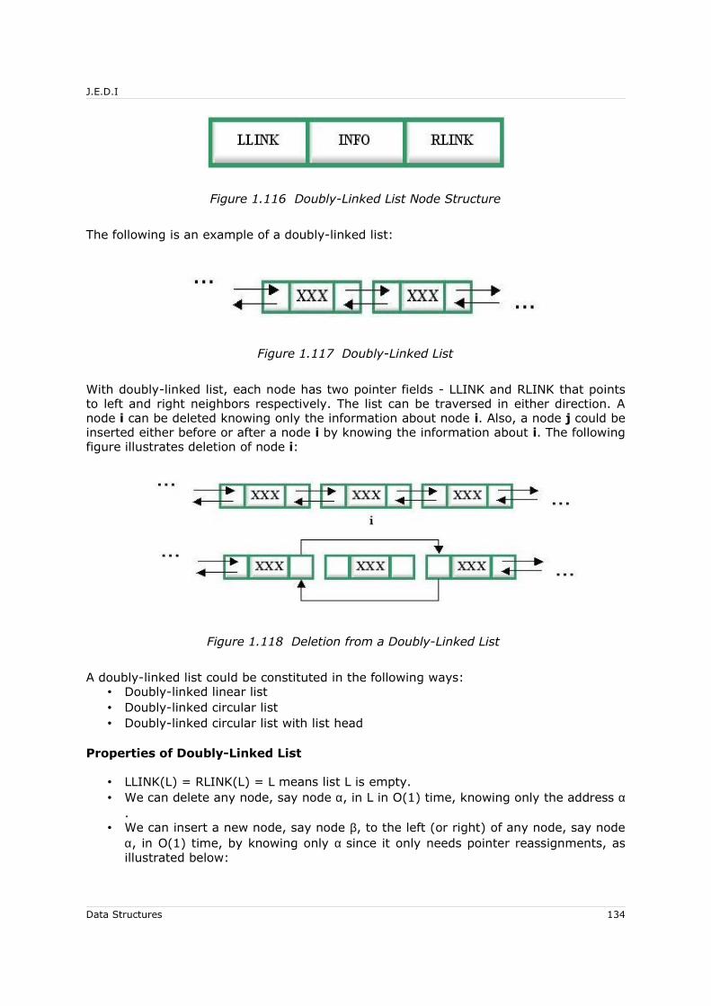
J.E.D.I

Figure 1.116 Doubly-Linked List Node Structure

The following is an example of a doubly-linked list:

Figure 1.117 Doubly-Linked List

With doubly-linked list, each node has two pointer fields - LLINK and RLINK that points to left and right neighbors respectively. The list can be traversed in either direction. A node i can be deleted knowing only the information about node i. Also, a node j could be inserted either before or after a node i by knowing the information about i. The following figure illustrates deletion of node i:

Figure 1.118 Deletion from a Doubly-Linked List

A doubly-linked list could be constituted in the following ways:• Doubly-linked linear list• Doubly-linked circular list• Doubly-linked circular list with list head

Properties of Doubly-Linked List

• LLINK(L) = RLINK(L) = L means list L is empty.• We can delete any node, say node α, in L in O(1) time, knowing only the address α

.• We can insert a new node, say node β, to the left (or right) of any node, say node

α, in O(1) time, by knowing only α since it only needs pointer reassignments, as illustrated below:

Data Structures 134

J.E.D.I

Figure 1.119 Insertion into a Doubly-Linked List

7.5 Application: Polynomial Arithmetic

Lists can be used to represent polynomials in which arithmetic operations can be applied. There are two issues that have to be dealt with:

• A way to represent the terms of a polynomial such that the entities comprising each term can be accessed and processed easily.

• A structure that is dynamic to grow and sink as needed.

To address these issues, singly-linked circular list with list head could be used, with a node structure as illustrated below:

Figure 1.120 Node Structure

where • EXPO field is divided into a sign (S) subfield and three exponent subfields for

variables x, y, z.• S is negative (-) if it is the list head, otherwise it is positive• ex, ey, ez are for the powers of the variables x, y and z respectively

• COEF field may contain any real number, signed or unsigned.

For example, the following is the list representation of the polynomial P(x,y,z) = 20x5y4 – 5x2yz + 13yz3:

Data Structures 135

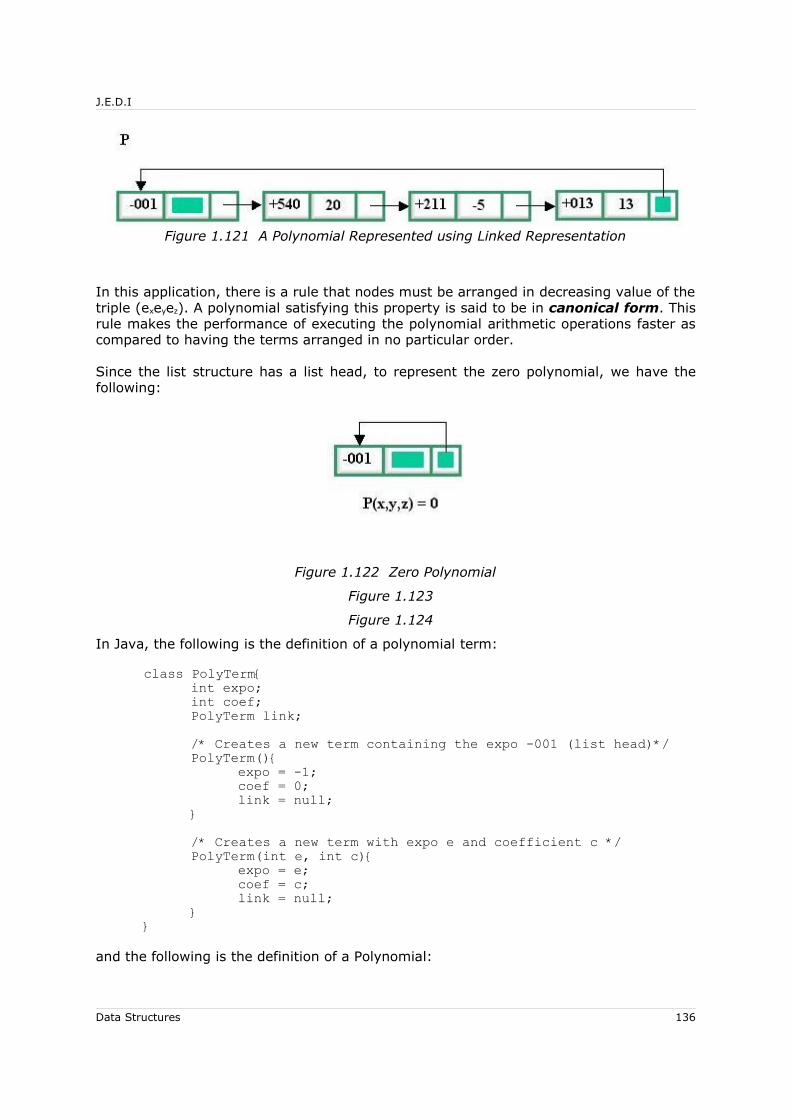
J.E.D.I

Figure 1.121 A Polynomial Represented using Linked Representation

In this application, there is a rule that nodes must be arranged in decreasing value of the triple (exeyez). A polynomial satisfying this property is said to be in canonical form. This rule makes the performance of executing the polynomial arithmetic operations faster as compared to having the terms arranged in no particular order.

Since the list structure has a list head, to represent the zero polynomial, we have the following:

Figure 1.122 Zero Polynomial

Figure 1.123

Figure 1.124

In Java, the following is the definition of a polynomial term:

class PolyTerm{int expo;int coef;PolyTerm link;/* Creates a new term containing the expo -001 (list head)*/PolyTerm(){

expo = -1;coef = 0;link = null;

}/* Creates a new term with expo e and coefficient c */PolyTerm(int e, int c){

expo = e;coef = c;link = null;

}}

and the following is the definition of a Polynomial:

Data Structures 136

J.E.D.I

class Polynomial{PolyTerm head = new PolyTerm(); /* list head */Polynomial(){

head.link = head;}/* Creates a new polynomial with head h */Polynomial(PolyTerm h){

head = h;h.link = head;

}}

To insert terms in canonical form, the following is a method of the class Polynomial:

/* Inserts a term to [this] polynomial by inserting in its proper location to maintain canonical form */void insertTerm(PolyTerm p){

PolyTerm alpha = head.link; /* roving pointer */PolyTerm beta = head;if (alpha == head){

head.link = p;p.link = head;return;

}else{

while (true){/* If the current term is less than alpha or

is the least in the polynomial, then insert */if ((alpha.expo < p.expo) || (alpha == head)){

p.link = alpha;beta.link = p;return;

}/* Advance alpha and beta */alpha = alpha.link;beta = beta.link;/* If have come full circle, return */if (beta == head) return;

}}

}

7.5.1 Polynomial Arithmetic Algorithms

This section covers how polynomial addition, subtraction and multiplication can be implemented using the structure just described.

Data Structures 137

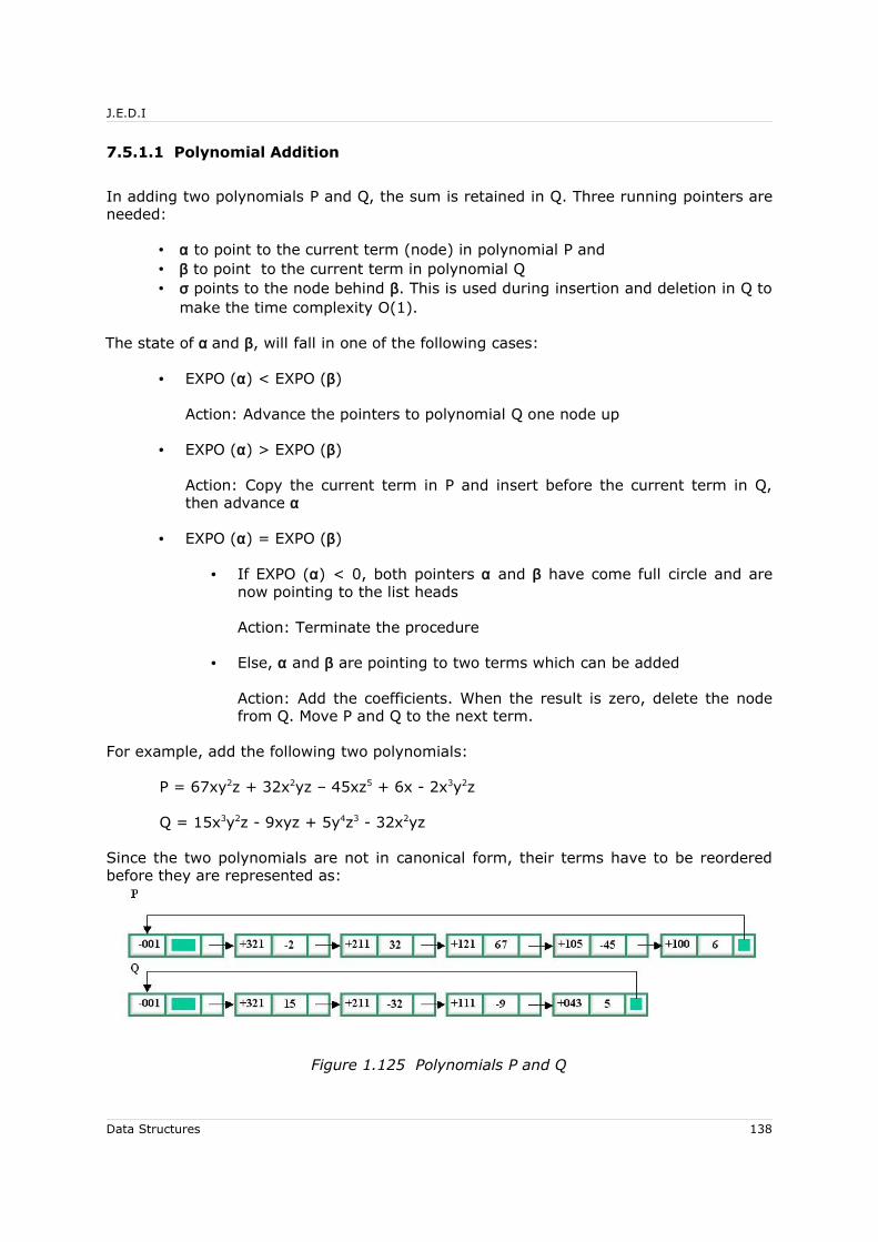
J.E.D.I

7.5.1.1 Polynomial Addition

In adding two polynomials P and Q, the sum is retained in Q. Three running pointers are needed:

• α to point to the current term (node) in polynomial P and• β to point to the current term in polynomial Q• σ points to the node behind β. This is used during insertion and deletion in Q to

make the time complexity O(1).

The state of α and β, will fall in one of the following cases:

• EXPO (α) < EXPO (β)

Action: Advance the pointers to polynomial Q one node up

• EXPO (α) > EXPO (β)

Action: Copy the current term in P and insert before the current term in Q, then advance α

• EXPO (α) = EXPO (β)

• If EXPO (α) < 0, both pointers α and β have come full circle and are now pointing to the list heads

Action: Terminate the procedure

• Else, α and β are pointing to two terms which can be added

Action: Add the coefficients. When the result is zero, delete the node from Q. Move P and Q to the next term.

For example, add the following two polynomials:

P = 67xy2z + 32x2yz – 45xz5 + 6x - 2x3y2z

Q = 15x3y2z - 9xyz + 5y4z3 - 32x2yz

Since the two polynomials are not in canonical form, their terms have to be reordered before they are represented as:

Figure 1.125 Polynomials P and Q

Data Structures 138

J.E.D.I

Adding the two,

Expo(α) = Expo(β)

adding α and β:

Expo(α) = Expo(β)

adding α and β results to deleting the node pointed to by β:

Expo(α) > Expo(β)

insert α between σ and β:

Data Structures 139

J.E.D.I

Expo(α) < Expo(β), advance σ and β:

Expo(α) > Expo(β), insert α into Q:

Expo(α) > Expo(β), insert α into Q:

Figure 1.126 Addition of Polynomials P and Q

Since both P and Q are in canonical form, one pass is sufficient. If the operands are not in canonical form, the procedure will not yield the correct result. If P has m terms and Q has n terms, the time complexity of the algorithm is O(m+n).

With this algorithm, there is no need for special handling of the zero polynomial. It works with zero P and/or Q. However, since the sum is retained in Q, it has to be duplicated if the need to use Q after the addition will arise. It could be done by calling the method add(Q, P) of class Polynomial, where P is initially the zero polynomial and will contain the duplicate of Q.

The following is the Java implementation of this procedure:

/* Performs the operation Q = P + Q, Q is [this] polynomial */void add(Polynomial P){

/* Roving pointer in P */PolyTerm alpha = P.head.link;/* Roving pointer in Q */PolyTerm beta = head.link;/* Pointer to the node behind beta, used in insertion to Q*/

Data Structures 140

J.E.D.I

PolyTerm sigma = head;PolyTerm tau;while (true){

/* Current term in P > current term in Q */if (alpha.expo < beta.expo) {

/* Advance pointers in Q */sigma = beta;beta = beta.link;

}else if (alpha.expo > beta.expo) {

/* Insert the current term in P to Q */tau = new PolyTerm();tau.coef = alpha.coef;tau.expo = alpha.expo;sigma.link = tau;tau.link = beta;sigma = tau;alpha = alpha.link; /* Advance pointer in P */

}else { /* Terms in P and Q can be added */

if (alpha.expo < 0) return; /* The sum is already in Q */else{

beta.coef = beta.coef + alpha.coef;/* If adding will cause to cancel out

the term */if (beta.coef == 0){

//tau = beta;sigma.link = beta.link;beta = beta.link;

}else{ /* Advance pointers in Q */

sigma = beta;beta = beta.link;

}/* Advance pointer in P */alpha = alpha.link;

}}

}}

7.5.1.2 Polynomial Subtraction

Subtraction of a polynomial Q from P, i.e., Q = P-Q, is simply polynomial addition with each term in Q negated: Q = P + (-Q). This could be done by traversing Q and negating the coefficients in the process before calling polyAdd.

/* Performs the operation Q = Q-P, Q is [this] polynomial */void subtract(Polynomial P){

PolyTerm alpha = P.head.link;

Data Structures 141

J.E.D.I

/* Negate every term in P */while (alpha.expo != -1) {

alpha.coef = - alpha.coef;alpha = alpha.link;

}/* Add P to [this] polynomial */this.add(P);/* Restore P */while (alpha.expo != -1) {

alpha = alpha.link;alpha.coef = - alpha.coef;

}}

7.5.1.3 Polynomial Multiplication

In multiplying two polynomials P and Q, an initially zero polynomial R is needed to contain the product, i.e. R = R + P*Q. In the process, every term in P is multiplied with every term in Q.

The following is the Java implementation:

/* Performs the operation R = R + P*Q, where T is initially a zero polynomial and R is this polynomial */

void multiply(Polynomial P, Polynomial Q){

/* Create temporary polynomial T to contain product term */Polynomial T = new Polynomial();

/* Roving pointer in T */PolyTerm tau = new PolyTerm();

/* To contain the product */Polynomial R = new Polynomial();

/* Roving pointers in P and Q */PolyTerm alpha, beta;

/* Initialize T and tau */T.head.link = tau;tau.link = T.head;

/* Multiply */alpha = P.head.link;

/* For every term in P... */while (alpha.expo != -1){

beta = Q.head.link;

/* ... multiply with every term in Q */while (beta.expo != -1){

tau.coef = alpha.coef * beta.coef;tau.expo = expoAdd(alpha.expo, beta.expo);

Data Structures 142

J.E.D.I

R.add(T);beta = beta.link;

}alpha = alpha.link;

}

this.head = R.head; /* Make [this] polynomial be R */

}

/* Performs addition of exponents of the triple(x,y,z) Auxillary method used by multiply */int expoAdd(int expo1, int expo2){

int ex = expo1/100 + expo2/100;int ey = expo1%100/10 + expo2%100/10;int ez = expo1%10 + expo2%10;

return (ex * 100 + ey * 10 + ez);}

7.6 Dynamic Memory Allocation

Dynamic memory allocation (DMA) refers to the management of a contiguous area of memory, called the memory pool, using techniques for block allocation and deallocation. It is assumed that the memory pool consists of individually addressable units called words. The size of a block is measured in words. Dynamic memory allocation is also known as dynamic storage allocation. In DMA, blocks are variable in size, hence, getNode and retNode, as discussed in Chapter 1, are not sufficient to manage allocation of blocks.

There are two operations related to DMA: reservation and liberation. During reservation, a block of memory is allocated to a requesting task. When a block is no longer needed, it has to be liberated. Liberation is the process of returning it to the memory pool.

There are two general techniques in dynamic memory allocation – sequential fit methods and buddy-system methods.

7.6.1 Managing the Memory Pool

There is a need to manage the memory pool since blocks could be allocated and deallocated as needed. Problem arises after a sequence of allocation and deallocation. That is, when the memory pool consist of free blocks scattered all over the pool between reserved blocks. In such a case, linked lists could be used to organize free blocks so that reservation and liberation can be done efficiently.

In sequential-fit methods, all free blocks are constituted in a singly-linked list called the avail list. In buddy-system methods, blocks are allocated in quantum sizes only, e.g. 1, 2, 4, 2k words only. Thus, several avail lists are maintained, one for each allowable size.

Data Structures 143

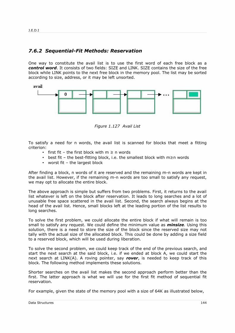
J.E.D.I

7.6.2 Sequential-Fit Methods: Reservation

One way to constitute the avail list is to use the first word of each free block as a control word. It consists of two fields: SIZE and LINK. SIZE contains the size of the free block while LINK points to the next free block in the memory pool. The list may be sorted according to size, address, or it may be left unsorted.

Figure 1.127 Avail List

To satisfy a need for n words, the avail list is scanned for blocks that meet a fitting criterion:

• first fit – the first block with m ≥ n words • best fit – the best-fitting block, i.e. the smallest block with m≥n words• worst fit – the largest block

After finding a block, n words of it are reserved and the remaining m-n words are kept in the avail list. However, if the remaining m-n words are too small to satisfy any request, we may opt to allocate the entire block.

The above approach is simple but suffers from two problems. First, it returns to the avail list whatever is left on the block after reservation. It leads to long searches and a lot of unusable free space scattered in the avail list. Second, the search always begins at the head of the avail list. Hence, small blocks left at the leading portion of the list results to long searches.

To solve the first problem, we could allocate the entire block if what will remain is too small to satisfy any request. We could define the minimum value as minsize. Using this solution, there is a need to store the size of the block since the reserved size may not tally with the actual size of the allocated block. This could be done by adding a size field to a reserved block, which will be used during liberation.

To solve the second problem, we could keep track of the end of the previous search, and start the next search at the said block, i.e. if we ended at block A, we could start the next search at LINK(A). A roving pointer, say rover, is needed to keep track of this block. The following method implements these solutions.

Shorter searches on the avail list makes the second approach perform better than the first. The latter approach is what we will use for the first fit method of sequential fit reservation.

For example, given the state of the memory pool with a size of 64K as illustrated below,

Data Structures 144

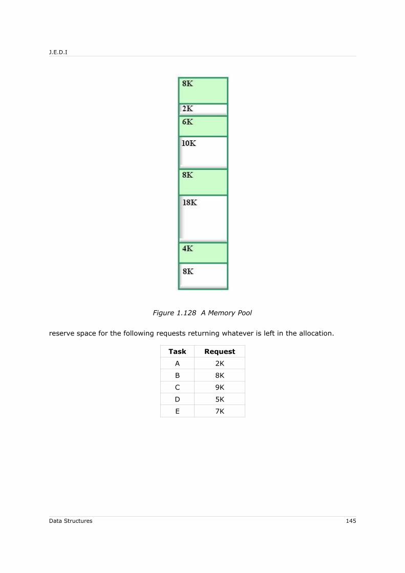
J.E.D.I

Figure 1.128 A Memory Pool

reserve space for the following requests returning whatever is left in the allocation.

Task Request

A 2K

B 8K

C 9K

D 5K

E 7K

Data Structures 145

J.E.D.I

Figure 1.129 Result of Applying the Three Sequential Fit Methods

The best-fit method reserves large blocks for later requests while in worst-fit, the largest block is allocated to return bigger available blocks to the avail list. In the best-fit method, there is a need to search the entire list to find the best-fitting block. Just like first-fit, there is also a tendency for too small blocks to accumulate, but can be minimized by using minsize. Best-fit does not necessarily mean producing better results than first-fit. Some investigations even showed that there are many cases in which first-fit outperforms best-fit. In some applications, worst-fit produce the best results among the three methods.

7.6.3 Sequential-Fit Methods: Liberation

When a reserved block is no longer needed, it has to be liberated. During liberation, adjacent free blocks must be collapsed into one to form a larger block (collapsing problem). This is an important consideration in sequential-fit liberation.

The following figure shows the four possible cases during liberation of a block:

(A) (A) (A) (A)

Data Structures 146

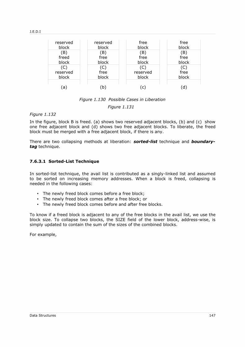
J.E.D.I

reserved block

reserved block

freeblock

freeblock

(B)freedblock

(B)freeblock

(B)freeblock

(B)freeblock

(C)reserved

block

(C)freeblock

(C)reserved

block

(C)freeblock

(a) (b) (c) (d)

Figure 1.130 Possible Cases in Liberation

Figure 1.131

Figure 1.132

In the figure, block B is freed. (a) shows two reserved adjacent blocks, (b) and (c) show one free adjacent block and (d) shows two free adjacent blocks. To liberate, the freed block must be merged with a free adjacent block, if there is any.

There are two collapsing methods at liberation: sorted-list technique and boundary-tag technique.

7.6.3.1 Sorted-List Technique

In sorted-list technique, the avail list is contributed as a singly-linked list and assumed to be sorted on increasing memory addresses. When a block is freed, collapsing is needed in the following cases:

• The newly freed block comes before a free block;• The newly freed block comes after a free block; or• The newly freed block comes before and after free blocks.

To know if a freed block is adjacent to any of the free blocks in the avail list, we use the block size. To collapse two blocks, the SIZE field of the lower block, address-wise, is simply updated to contain the sum of the sizes of the combined blocks.

For example,

Data Structures 147

J.E.D.I

Data Structures 148

J.E.D.I

Figure 1.133 Examples of Liberation

Data Structures 149

J.E.D.I

7.6.3.2 Boundary-Tag Technique

Boundary tag technique uses two control words and double linking. The first and the last words contain control details. The following figure shows the link structure and the two states of a block (reserved and free):

(a) free block

(b) reserved block

Figure 1.134 Node Strucuture in Boundary-Tag Technique

The value of TAG is 0 if the block is free, otherwise it is 1. Two TAG and SIZE fields are present to make merging of free blocks execute in O(1) time.

The avail list is constituted as a doubly-linked list with a list head. Initially, the avail list consists of just one block, the whole memory pool, bounded below and above by memory blocks not available for DMA. The following figure shows the initial state of the avail list:

Data Structures 150

J.E.D.I

Figure 1.135 The Initial State of the Memory Pool

After using the memory for some time, it will leave discontinuous segments, thus we have this avail list:

Figure 1.136 Avail List after Several Allocations and Deallocations

Sorted-list technique is in O(m), where m is the number of blocks in the avail list. Boundary-tag technique has time complexity O(1).

Data Structures 151

J.E.D.I

7.6.4 Buddy-System Methods

In buddy-system methods, blocks are allocated in quantum sizes. Several avail lists, one for each allowable size, are maintained. There are two buddy system methods:

• Binary buddy-system method – blocks are allocated in sizes based on the powers of two: 1, 2, 4, 8, …, 2k words

• Fibonacci buddy-system method – blocks are allocated in sizes based on the Fibonacci number sequence: 1, 2, 3, 5, 8, 13, … (k-1)+(k-2) words

In this section, we will cover binary buddy-system method only.

7.6.4.1 Binary Buddy-System Method

Figure 1.137 Buddies in the Binary Buddy-System

7.6.4.2 Reservation

Given a block with size 2k, the following is the algorithm for reserving a block for a request for n words:

1. If the current block’s size < n:

• If the current block is the largest size, return: No sufficiently large block is available.

• Else go to the avail list of the block next in size. Go to 1.

• Else, go to 2.

2. If the block’s size is the smallest multiple of 2 ≥ n, then reserve the block for the requesting task. Return. Else go to 3.

3. Divide the block into two parts. These two are called buddies. Go to 2, having the upper half of the newly cut buddies as the current block.

For example, reserve space for the requests A (7K), B (3K), C (16K), D (8K), and E

Data Structures 152

J.E.D.I

(15K) from an unused memory pool of size 64K.

Data Structures 153

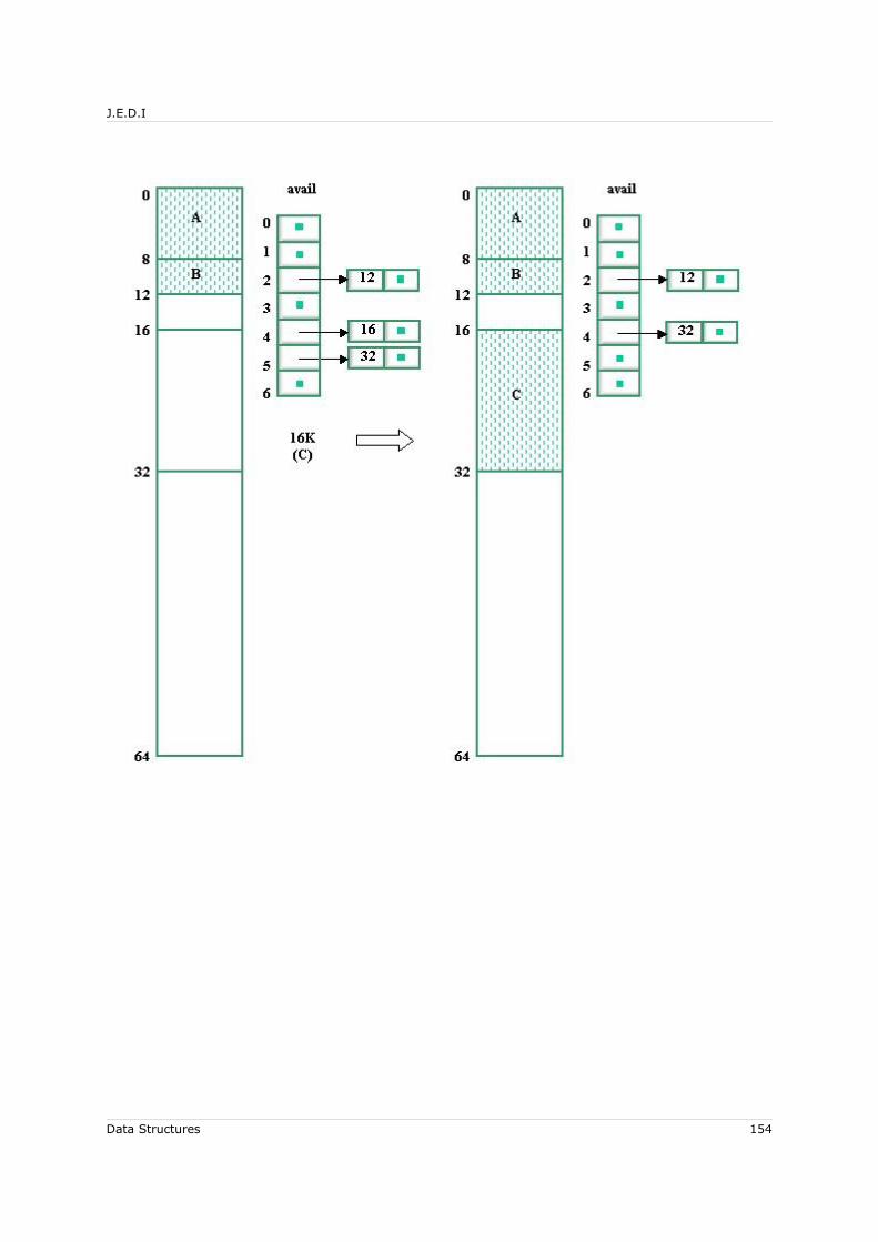
J.E.D.I

Data Structures 154

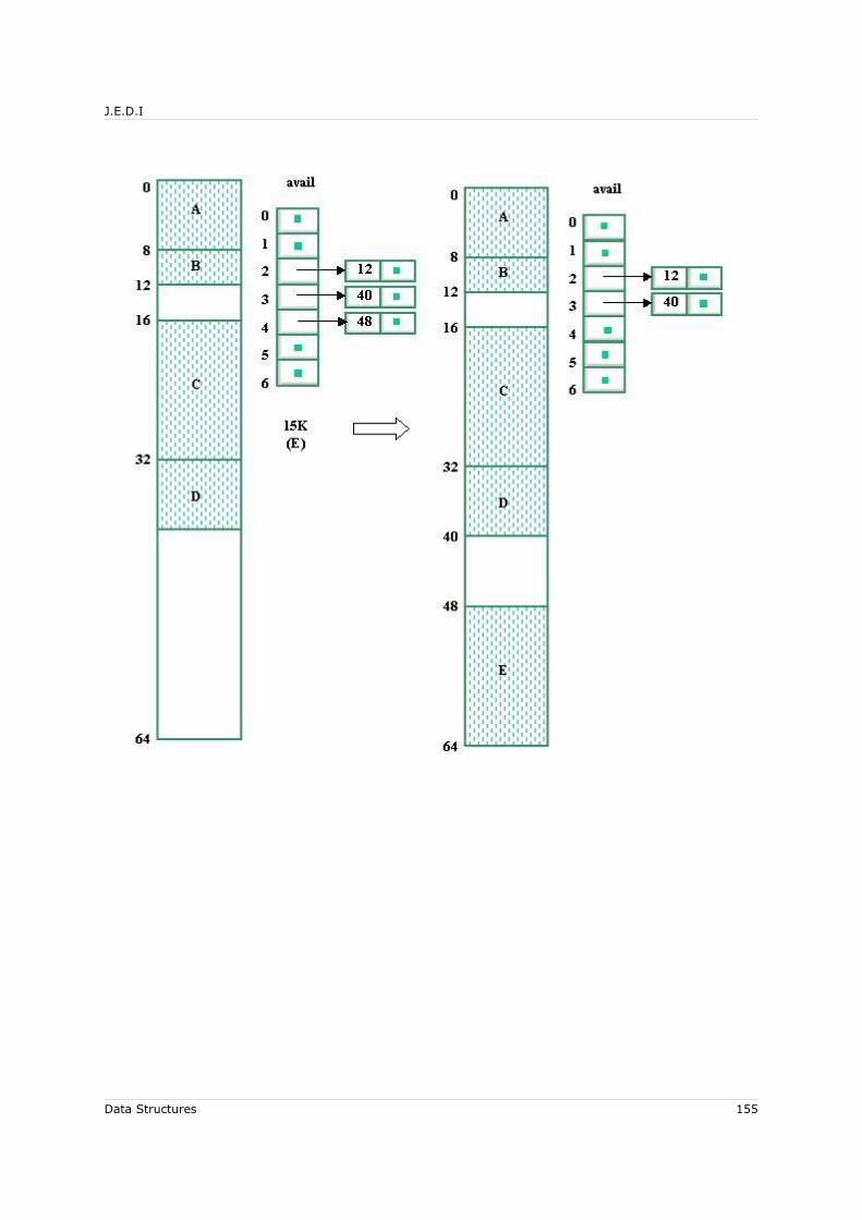
J.E.D.I

Data Structures 155

J.E.D.I

Figure 1.138 Binary Buddy System Method Reservation Example

Data Structures 156

J.E.D.I

Liberation

When a block is freed by a task and if the buddy of the block being freed is free, collapsing of the buddies is needed. When the newly collapsed block’s buddy is also free, collapsing is performed again. This is done repeatedly until no buddies can be collapsed anymore.

Locating the buddy is a crucial step in the liberation operation and is done by computation:

Let β(k:α) = address of the buddy of the block of size 2k at address α

β(k:α) = α + 2k if α mod 2k+1 = 0

β(k:α) = α - 2k otherwise

If the located buddy happens to be free, it can be collapsed with the newly-freed block. For the buddy-system method to be efficient, there is a need to maintain one avail list for each allowable size. The following is the algorithm for reservation using binary buddy system method:

1. If a request for n words is made and the avail list for blocks of size 2k, where k = log2n, is not empty, then we get a block from the avail list. Otherwise, go to 2.

2. Get a block from the avail list of size 2p where p is the smallest integer greater than k for which the list is not empty.

3. Split the block p-k times, inserting unused blocks in their respective avail lists.

Using the previous allocation as our example, liberate the blocks with reservation B (3K), D (8K), and A (7K) in the order given.

Data Structures 157

J.E.D.I

Figure 1.139 Binary Buddy System Method Liberation Example

Figure 1.140

Data Structures 158

J.E.D.I

In the implementation, the following node structure, a doubly-linked list, will be used for the avail lists:

LLINK TAG KVAL RLINKTAG = 0 if free block 1 if reserved blockKVAL = k if block has size 2k

To initialize the memory pool for the buddy-system method, assume that it is of size 2m. There is a need to maintain m+1 lists. The pointers avail(0:m) to the lists are stored in an array of size m+1.

7.6.5 External and Internal Fragmentation in DMA

After a series of reservation and splitting, blocks of size too small to satisfy any request remain in the avail list. Being too small, it has a very slim chance to be reserved, and will eventually be scattered in the avail list. This results to long searches. Also, even if the sizes sum up to a value that could satisfy a request, they could not be utilized since they are scattered all over the memory pool. This is what is referred to as external fragmentation. This is solved in sequential-fit methods by using minsize, wherein an entire block is reserved if what will remain in the allocation is less than the specified value. During liberation, this is addressed by collapsing free, adjacent blocks.

The approach of using minsize in sequential-fit methods or rounding off requests to 2log2n

in binary buddy-system method, leads to 'overallocation' of space. This allocation of space to tasks more than what they need results in what is known as internal fragmentation.

7.7 Summary

• A list is a finite set of zero or more elements that may be atoms or lists

• Singly-linked linear lists may be represented using sequential or linked representation. Other list representations are singly-linked circular list, singly-linked list with header nodes and doubly-linked list

• Lists can be used to represent polynomials in which arithmetic operations can be applied

• Dynamic memory allocation refers to the management of the memory pool using techniques for block allocation and deallocation

• Both DMA techniques sequential fit and buddy-system may suffer from internal or external fragmentation

Data Structures 159

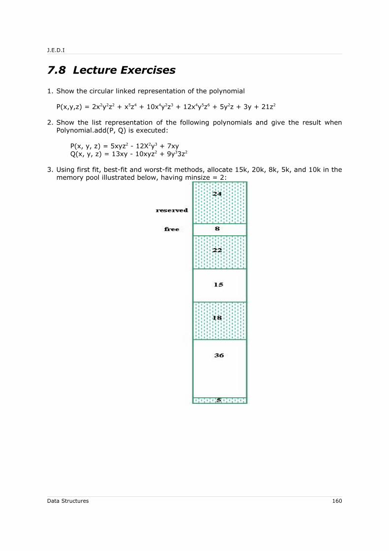
J.E.D.I


1. Show the circular linked representation of the polynomial

P(x,y,z) = 2x2y2z2 + x5z4 + 10x4y2z3 + 12x4y5z6 + 5y2z + 3y + 21z2

2. Show the list representation of the following polynomials and give the result when Polynomial.add(P, Q) is executed:

P(x, y, z) = 5xyz2 - 12X2y3 + 7xyQ(x, y, z) = 13xy - 10xyz2 + 9y33z2

3. Using first fit, best-fit and worst-fit methods, allocate 15k, 20k, 8k, 5k, and 10k in the memory pool illustrated below, having minsize = 2:

Data Structures 160

J.E.D.I

4. Using binary buddy-system method and given an empty memory pool of size 128K, reserve space for the following requests:

Task Request

A 30K

B 21K

C 13K

D 7K

E 14K

Show the state of the memory pool after each allocation. There is no need to show the avail lists. Liberate C, E and D in the order given. Perform merging when necessary. Show how the buddies are obtained.


1. Create a Java interface containing the operations insert, delete, isEmpty, size, update, append two lists and search.

2. Write a Java class definition that implements the interface created in 1 using doubly-linked linear list.

3. Write a Java class that makes use of Node to create a generalized list.

4. Create a Java interface containing the operations insert, delete, isEmpty, size, update, append two lists and search.

5. Write a Java class definition that implements the interface created in 1 using doubly-linked linear list.

6. Write a Java class that makes use of Node to create a generalized list.

7. Create a Java interface that contains the basic operations of a list - finding the length, deletion, update, insertion and search.

8.9. By implementing the interface created in (1), create a class for

a) a singly-linked list

b) a circular-list

c) a doubly-linked list

Data Structures 161

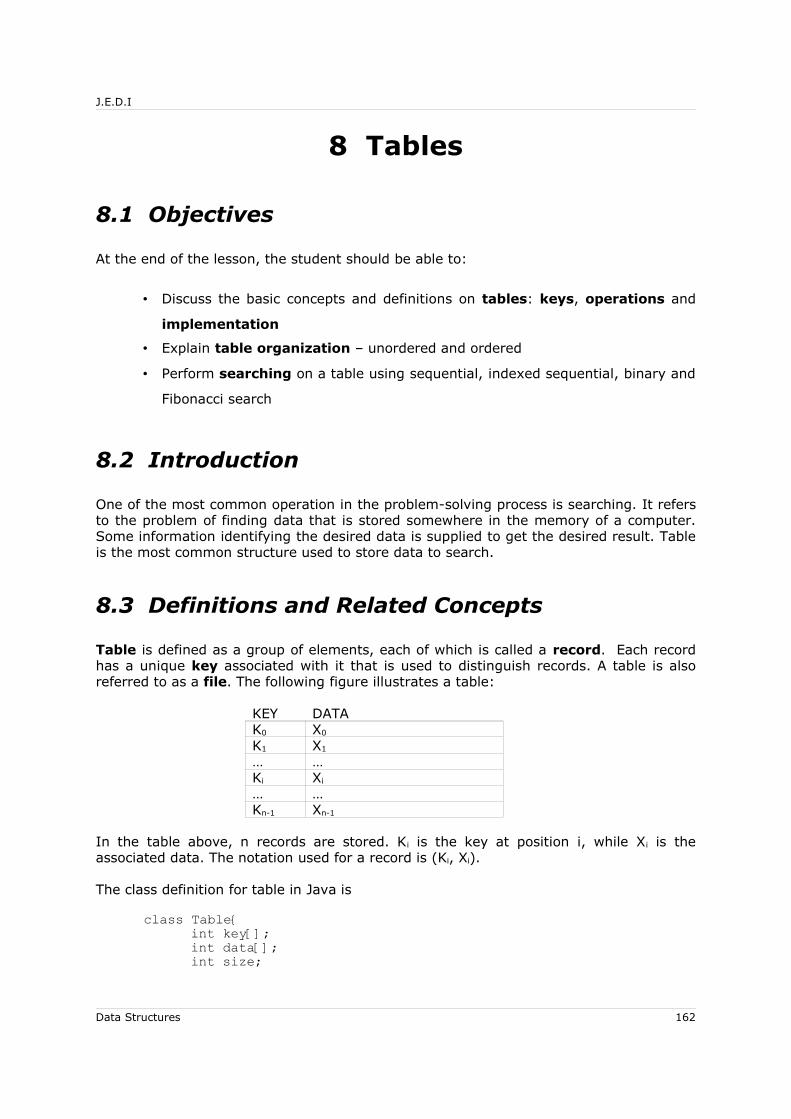
J.E.D.I

8 Tables

8.1 Objectives


• Discuss the basic concepts and definitions on tables: keys, operations and

implementation

• Explain table organization – unordered and ordered

• Perform searching on a table using sequential, indexed sequential, binary and

Fibonacci search

8.2 Introduction

One of the most common operation in the problem-solving process is searching. It refers to the problem of finding data that is stored somewhere in the memory of a computer. Some information identifying the desired data is supplied to get the desired result. Table is the most common structure used to store data to search.


Table is defined as a group of elements, each of which is called a record. Each record has a unique key associated with it that is used to distinguish records. A table is also referred to as a file. The following figure illustrates a table:

KEY DATAK0 X0

K1 X1

… …Ki Xi

… …Kn-1 Xn-1

In the table above, n records are stored. Ki is the key at position i, while Xi is the associated data. The notation used for a record is (Ki, Xi).

The class definition for table in Java is

class Table{int key[];int data[];int size;

Data Structures 162

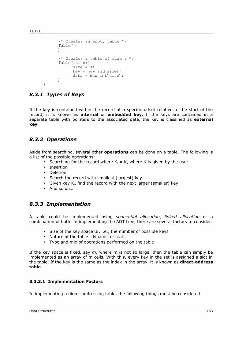
J.E.D.I

/* Creates an empty table */Table(){}/* Creates a table of size s */Table(int s){

size = s;key = new int[size];data = new int[size];

}}

8.3.1 Types of Keys

If the key is contained within the record at a specific offset relative to the start of the record, it is known as internal or embedded key. If the keys are contained in a separate table with pointers to the associated data, the key is classified as external key.

8.3.2 Operations

Aside from searching, several other operations can be done on a table. The following is a list of the possible operations:

• Searching for the record where Ki = K, where K is given by the user• Insertion• Deletion• Search the record with smallest (largest) key• Given key Ki, find the record with the next larger (smaller) key• And so on…

8.3.3 Implementation

A table could be implemented using sequential allocation, linked allocation or a combination of both. In implementing the ADT tree, there are several factors to consider:

• Size of the key space Uk, i.e., the number of possible keys• Nature of the table: dynamic or static• Type and mix of operations performed on the table

If the key space is fixed, say m, where m is not so large, then the table can simply be implemented as an array of m cells. With this, every key in the set is assigned a slot in the table. If the key is the same as the index in the array, it is known as direct-address table.

8.3.3.1 Implementation Factors

In implementing a direct-addressing table, the following things must be considered:

Data Structures 163

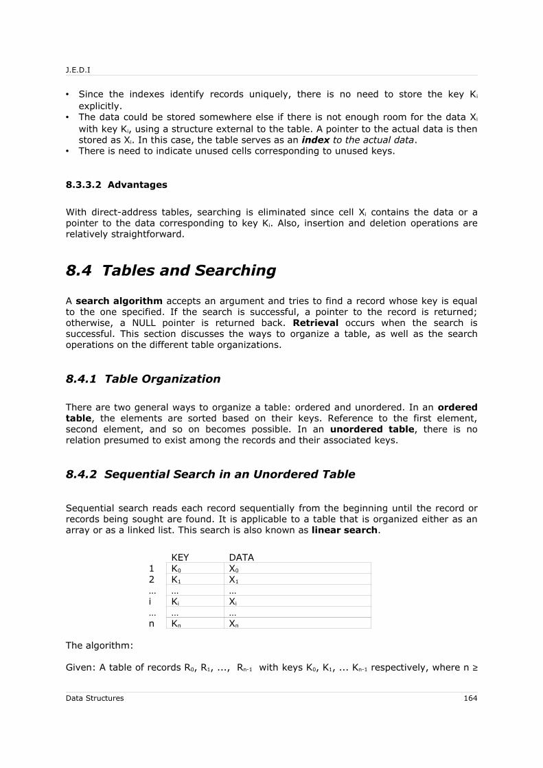
J.E.D.I

• Since the indexes identify records uniquely, there is no need to store the key Ki

explicitly.• The data could be stored somewhere else if there is not enough room for the data Xi

with key Ki, using a structure external to the table. A pointer to the actual data is then stored as Xi. In this case, the table serves as an index to the actual data.

• There is need to indicate unused cells corresponding to unused keys.

8.3.3.2 Advantages

With direct-address tables, searching is eliminated since cell Xi contains the data or a pointer to the data corresponding to key Ki. Also, insertion and deletion operations are relatively straightforward.

8.4 Tables and Searching

A search algorithm accepts an argument and tries to find a record whose key is equal to the one specified. If the search is successful, a pointer to the record is returned; otherwise, a NULL pointer is returned back. Retrieval occurs when the search is successful. This section discusses the ways to organize a table, as well as the search operations on the different table organizations.

8.4.1 Table Organization

There are two general ways to organize a table: ordered and unordered. In an ordered table, the elements are sorted based on their keys. Reference to the first element, second element, and so on becomes possible. In an unordered table, there is no relation presumed to exist among the records and their associated keys.

8.4.2 Sequential Search in an Unordered Table

Sequential search reads each record sequentially from the beginning until the record or records being sought are found. It is applicable to a table that is organized either as an array or as a linked list. This search is also known as linear search.

KEY DATA1 K0 X0

2 K1 X1

… … …i Ki Xi

… … …n Kn Xn

The algorithm:

Given: A table of records R0, R1, ..., Rn-1 with keys K0, K1, ... Kn-1 respectively, where n ≥

Data Structures 164

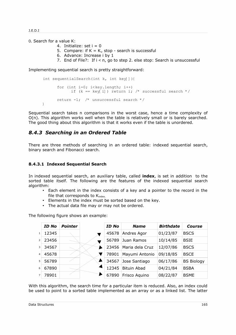
J.E.D.I

0. Search for a value K:4. Initialize: set i = 05. Compare: if K = Ki, stop - search is successful6. Advance: Increase i by 1 7. End of File?: If i < n, go to step 2. else stop: Search is unsuccessful

Implementing sequential search is pretty straightforward:

int sequentialSearch(int k, int key[]){for (int i=0; i<key.length; i++)

if (k == key[i]) return i; /* successful search */return -1; /* unsuccessful search */

}

Sequential search takes n comparisons in the worst case, hence a time complexity of O(n). This algorithm works well when the table is relatively small or is barely searched. The good thing about this algorithm is that it works even if the table is unordered.

8.4.3 Searching in an Ordered Table

There are three methods of searching in an ordered table: indexed sequential search, binary search and Fibonacci search.

8.4.3.1 Indexed Sequential Search

In indexed sequential search, an auxiliary table, called index, is set in addition to the sorted table itself. The following are the features of the indexed sequential search algorithm:

• Each element in the index consists of a key and a pointer to the record in the file that corresponds to Kindex.

• Elements in the index must be sorted based on the key.• The actual data file may or may not be ordered.

The following figure shows an example:

ID No Pointer ID No Name Birthdate Course

1 12345 45678 Andres Agor 01/23/87 BSCS

2 23456 56789 Juan Ramos 10/14/85 BSIE

3 34567 23456 Maria dela Cruz 12/07/86 BSCS

4 45678 78901 Mayumi Antonio 09/18/85 BSCE

5 56789 34567 Jose Santiago 06/17/86 BS Biology

6 67890 12345 Bituin Abad 04/21/84 BSBA

7 78901 67890 Frisco Aquino 08/22/87 BSME

With this algorithm, the search time for a particular item is reduced. Also, an index could be used to point to a sorted table implemented as an array or as a linked list. The latter

Data Structures 165

J.E.D.I

implementation implies a larger space overhead for pointers but insertions and deletions can be performed immediately.

8.4.3.2 Binary Search

Binary search begins with an interval covering the whole table, that is the middle value. If the search value is less than the item in the middle of the interval, the interval is narrowed down to the lower half. Otherwise, it is narrowed down to the upper half. This process of reducing the search size by half is repeatedly performed until the value is found or the interval is empty. The algorithm for the binary search makes use of the following relations in searching for the key K:

• K = Ki : stop, the desired record is found• K < Ki : search the lower half - records with keys K1 to Ki-1

• K > Ki : search the upper half - records with keys Ki+1 to Kn

where i is initially the middle index value.

The Algorithm

/* Returns the index of key k if found, otherwise -1 */int binarySearch(int k, Table t){

int lower = 0;int upper = t.size - 1;int middle;while (lower < upper){

/* get middle */middle = (int) Math.floor((lower + upper) / 2);/* successful search */if (k == t.key[middle]) return middle;/* discard lower half */else if (k > t.key[middle]) lower = middle + 1;/* discard upper half */else upper = upper - 1;

}return(-1); /* unsuccessful search */

}

For example, search for the key k=34567:

0 1 2 3 4 5 6

12345 23456 34567 45678 56789 67890 78901

lower = 0, upper = 6, middle = 3: k < kmiddle (45678)

lower = 0, upper = 2, middle = 1: k > kmiddle (23456)

Data Structures 166

J.E.D.I

lower = 2, upper = 2, middle = 2: k = kmiddle (34567) ==> successful search

Since the search area is reduced logarithmically, i.e., halved each time the size is reduced, the time complexity of the algorithm is O(log2n). The algorithm may be used if the table uses indexed sequential organization. However, it can only be used with ordered tables stored as an array.

8.4.3.3 Multiplicative Binary Search

Multiplicative binary search is similar to the previous algorithm but avoids the division needed to find the middle key. To do that, there is a need to rearrange the records in the table:

1. Assign keys K1 < K2 < K3 < …< Kn to the nodes of a complete binary tree in inorder sequence

2. Arrange the records in the table according to the corresponding level-order sequence in the binary tree.

The Search Algorithm

The comparison begins at the root of the binary tree, j=0, which is the middle key in the original table.

/* Accepts a set of keys represented as a complete binary tree */int multiplicativeBinarySearch(int k, int key[]){

int i = 0;while (i < key.length){

if (k == key[i]) return i; /* successful search */else if (k < key[i]) i = 2 * i + 1; /* go left */else i = 2 * i + 2; /* go right */

}return -1; /* unsuccessful search */

}

Since computation for the middle element is eliminated, multiplicative binary search is faster than the traditional binary search. However, there is a need to rearrange the given set of keys before the algorithm can be applied.

8.4.3.4 Fibonacci Search

Fibonacci search uses the simple properties of the Fibonacci number sequence defined by the following recurrence relation:

F0 = 0F1 = 1 Fj = Fi-2 + Fi-1 , i ≥ 2

Data Structures 167

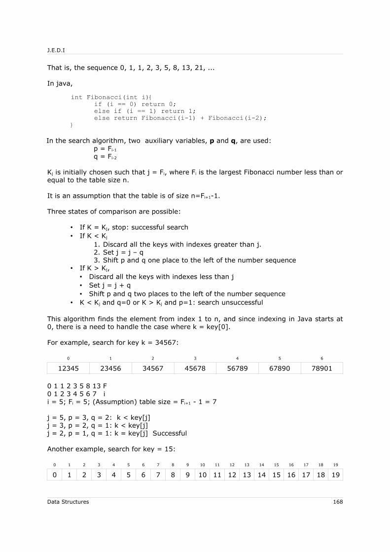
J.E.D.I

That is, the sequence 0, 1, 1, 2, 3, 5, 8, 13, 21, ...

In java,

int Fibonacci(int i){if (i == 0) return 0;else if (i == 1) return 1;else return Fibonacci(i-1) + Fibonacci(i-2);

}

In the search algorithm, two auxiliary variables, p and q, are used: p = Fi-1

q = Fi-2

Kj is initially chosen such that j = Fi, where Fi is the largest Fibonacci number less than or equal to the table size n.

It is an assumption that the table is of size n=Fi+1-1.

Three states of comparison are possible:

• If K = Kj, stop: successful search• If K < Kj

1. Discard all the keys with indexes greater than j. 2. Set j = j – q3. Shift p and q one place to the left of the number sequence

• If K > Kj, • Discard all the keys with indexes less than j• Set j = j + q• Shift p and q two places to the left of the number sequence

• K < Kj and q=0 or K > Kj and p=1: search unsuccessful

This algorithm finds the element from index 1 to n, and since indexing in Java starts at 0, there is a need to handle the case where k = key[0].

For example, search for key k = 34567:

0 1 2 3 4 5 6

12345 23456 34567 45678 56789 67890 78901

0 1 1 2 3 5 8 13 F0 1 2 3 4 5 6 7 ii = 5; Fi = 5; (Assumption) table size = Fi+1 - 1 = 7

j = 5, p = 3, q = 2: k < key[j] j = 3, p = 2, q = 1: k < key[j] j = 2, p = 1, q = 1: k = key[j] Successful

Another example, search for key = 15:

0 1 2 3 4 5 6 7 8 9 10 11 12 13 14 15 16 17 18 19

0 1 2 3 4 5 6 7 8 9 10 11 12 13 14 15 16 17 18 19

Data Structures 168

J.E.D.I

i = 7; Fi = 13; (Assumption) table size = Fi+1 - 1 = 20

j = 13; p = 8, q=5: k > key[j] j = 18; p = 3; q=2: k < key[j] j = 15; p = 2; q=1: k = key[j] Successful

The following is the algorithm:

int fibonacciSearch(int k, int key[]){int i;int F[] = new int[key.length];int temp;/* Find F(i), the largest Fibonacci number <= table size */for (i=0; i<key.length; i++){

F[i] = Fibonacci(i);if (key.length < F[i]) {

i--;break;

}}int p = F[i-1];int q = F[i-2];int j = F[i];if (k == key[0]) return 0;while (true){

if (k == key[j])return j; /* successful search */

else if (k < key[j])if (q == 0)

return -1; /* unsuccessful search */else { /* adjust i, p and q */

j = j - q;temp = p;p = q;q = temp - q;

}else

if (p == 1)return -1; /* unsuccessful search */

else{ /* adjust i, p and q */j = j + q;p = p - q;

q = q - p;}

}}

Data Structures 169

J.E.D.I

8.5 Summary

• A table is a group of elements, each of which is called a record

• Two types of keys are internal or embedded key, and external key

• Tables may be represented using sequential allocation, link allocation or both

• Searching is eliminated in direct-address table. Also, insertion and deletion are relatively straightforward

• A table may be ordered or unordered. Linear search is used if the table is unordered, while indexed sequential search, binary search or Fibonacci search is used if the table is ordered


Using the following methods of searching, a) Sequential Searchb) Multiplicative Binary Searchc) Binary Searchd) Fibonacci Search

Search for

1. A in S E A R C H I N G

2. D in W R T A D E Y S B

3. T in C O M P U T E R S


1. Extend the Java class defined in this chapter to contain methods for insertion at a specified location and deletion of an item with key K. Use sequential representation.

Data Structures 170

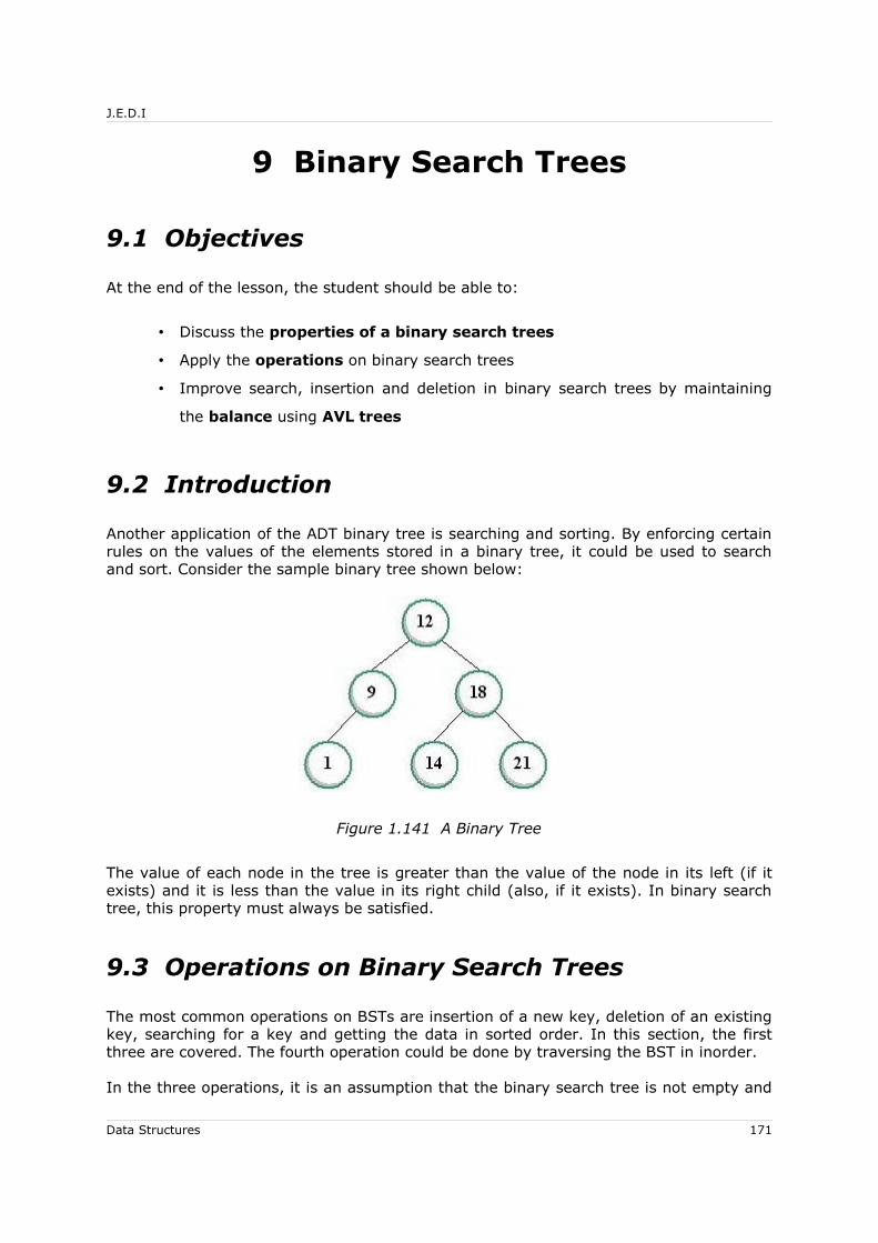
J.E.D.I

9 Binary Search Trees

9.1 Objectives


• Discuss the properties of a binary search trees

• Apply the operations on binary search trees

• Improve search, insertion and deletion in binary search trees by maintaining

the balance using AVL trees

9.2 Introduction

Another application of the ADT binary tree is searching and sorting. By enforcing certain rules on the values of the elements stored in a binary tree, it could be used to search and sort. Consider the sample binary tree shown below:

Figure 1.141 A Binary Tree

The value of each node in the tree is greater than the value of the node in its left (if it exists) and it is less than the value in its right child (also, if it exists). In binary search tree, this property must always be satisfied.

9.3 Operations on Binary Search Trees

The most common operations on BSTs are insertion of a new key, deletion of an existing key, searching for a key and getting the data in sorted order. In this section, the first three are covered. The fourth operation could be done by traversing the BST in inorder.

In the three operations, it is an assumption that the binary search tree is not empty and

Data Structures 171

J.E.D.I

it does not store multiple values. Also, the node structure BSTNode(left, info, right), as illustrated below, is used:

Figure 1.142 BSTNode

In Java,

class BSTNode {int info;BSTNode left, right;public BSTNode(){}public BSTNode(int i) {

info = i;}public BSTNode(int i, BSTNode l, BSTNode r) {

info = i;left = l;right = r;

}}

The binary search tree used in this lesson has a list head as illustrated in the following figure:

Figure 1.143 Linked Representation of the Binary Search Tree T2

If the binary search tree is empty, the left and right pointers of bstHead points to itself; otherwise, the right pointer points to the root of the tree. The following is the class definition of the bst using this structure:

class BST{

Data Structures 172

J.E.D.I

BSTNode bstHead = new BSTNode();/* Creates an empty bst */BST(){

bstHead.left = bstHead;bstHead.right = bstHead;

}/* Creates a bst with root r, pointed to by bstHead.right */BST(BSTNode r){

bstHead.left = bstHead;bstHead.right = r;

}}

9.3.1 Searching

In searching for a value, say k, three conditions are possible:

• k = value at the node (successful search)• k < value at the node (search the left subtree)• k > value at the node (search the right subtree)

The same process is repeated until a match is found or the farthest leaf is reached but no match is found. In the case of the latter, the search is unsuccessful.

The following is the Java implementation of the above algorithm:

/* Searches for k, returns the node containing k if found */BSTNode search(int k){

BSTNode p = bstHead.right; /* the root node *//* If the tree is empty, return null */if (p == bstHead) return null;/* Compare */while (true){

if (k == p.info) return p; /* successful search */else if (k < p.info) /* go left */

if (p.left != null) p = p.left;else return null; /* not found */

else /* go right */if (p.right != null) p = p.right;else return null; /* not found */

}}

9.3.2 Insertion

In inserting a value, searching is performed in finding its proper location in the tree. However, if during the search process the key is found, the insertion will not be performed. The following is the algorithm:

Data Structures 173

J.E.D.I

1. Start the search at the root node. Declare a node p and make it point to the root2. Do the comparison:

if (k == p.info) return false // if key found, insertion not allowedelse if (k < p.info) p = p.left // go left else p = p.right // if (k > p.info) go right

3. Insert the node (p now points to the new parent of node to insert):newNode.info = knewNode.left = nullnewNode.right = nullif (k < p.info) p.left = newNodeelse p.right = newNode

In Java,

/* Inserts k into the binary search tree */boolean insert(int k){

BSTNode p = bstHead.right; /* the root node */BSTNode newNode = new BSTNode();/* If the tree is empty, make the new node the root */if (p == bstHead){

newNode.info = k;bstHead.right = newNode;return true;

}/* Find the right place to insert k */while (true){

if (k == p.info) /* key already exists */return false;

else if (k < p.info) /* go left */if (p.left != null) p = p.left;else break;

else /* go right */if (p.right != null) p = p.right;else break;

}/* Insert the new key in its proper place */newNode.info = k;if (k < p.info) p.left = newNode;else p.right = newNode;return true;

}

9.3.3 Deletion

Deleting a key from the binary search tree is a bit more complex than the other two operations just discussed. The operation starts by finding the key to delete. If not found, the algorithm simply returns to tell that deletion fails. If the search returns a node, then there is a need to delete the node that contains the key that we searched for.

However, deletion is not as simple as removing the node found since it has a parent pointing to it. It is also a big possibility that it is the parent of some other nodes in the binary search tree. In this case, there is a need to have its children “adopted” by some other node, and the pointers pointing to it should also be adjusted. And in the process of

Data Structures 174

J.E.D.I

reassigning pointers, the BST property of the order of the key values has to be maintained.

There are two general cases to consider in deleting a node d:

1. Node d is an external node(leaf):

Action: update the child pointer of the parent p:if d is a left child, set p.left = null otherwise, set p.right = null

Figure 1.144 Deletion of a Leaf Node

2. Node is internal (there are two subcases):

Case 1: If d has a left subtree, 1. Get the inorder predecessor, ip. Inorder predecessor is defined as the

rightmost node in the left subtree of the current node, which in this case is d. It contains the preceding key if the BST is traversed in inorder.

2. Get the parent of ip, say p_ip. 3. Replace d with ip.4. Remove ip from its old location by adjusting the pointers:

a. If ip is not a leaf node:1. Set the right child of p_ip to point to the left child of ip2. Set the left child of ip to point to the left child of d

b. Set the right child of ip to point to the right child of d

Data Structures 175

J.E.D.I

Figure 1.145 Deletion of an Internal Node with a Left Subtree

Case 2: If d has no left son but with a right subtree

1. Get the inorder successor, is. Inorder successor is defined as the leftmost node in the right subtree of the current node. It contains the succeeding key if the BST is traversed in inorder.

2. Get the parent of is, say p_is. 3. Replace d with is.4. Remove is from its old location by adjusting the pointers:

a. If is is not a leaf node:3. Set the left child of p_is to point to the right child of is4. Set the right child of is to point to the right child of d

b. Set the left child of is to point to the left child of d

Data Structures 176

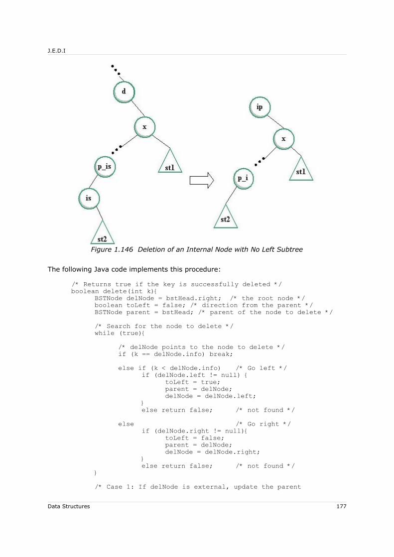
J.E.D.I

Figure 1.146 Deletion of an Internal Node with No Left Subtree

The following Java code implements this procedure:

/* Returns true if the key is successfully deleted */boolean delete(int k){

BSTNode delNode = bstHead.right; /* the root node */boolean toLeft = false; /* direction from the parent */BSTNode parent = bstHead; /* parent of the node to delete *//* Search for the node to delete */while (true){

/* delNode points to the node to delete */if (k == delNode.info) break;else if (k < delNode.info) /* Go left */

if (delNode.left != null) {toLeft = true;parent = delNode;delNode = delNode.left;

}else return false; /* not found */

else /* Go right */if (delNode.right != null){

toLeft = false;parent = delNode;delNode = delNode.right;

}else return false; /* not found */

}/* Case 1: If delNode is external, update the parent

Data Structures 177

J.E.D.I

& delete the node */if ((delNode.left == null) && (delNode.right == null)){

if (toLeft) parent.left = null;else parent.right = null;

}/* Case 2.1: If delNode is internal and has left son */else if (delNode.left != null) {

/* inorder predecessor */BSTNode inPre = delNode.left;/* parent of the inorder predecessor */BSTNode inPreParent = null;/* Find the inorder successor of delNode */while (inPre.right != null) {

inPreParent = inPre;inPre = inPre.right;

}/* Replace delNode with inPre */if (toLeft) parent.left = inPre;else parent.right = inPre;/* Remove inSuc from its original location *//* if inPre is not a leaf node */if (inPreParent != null) {

inPreParent.right = inPre.left;inPre.left = delNode.left;

}inPre.right = delNode.right;

}/* Case 2.2: If delNode is internal and

has no left son but with right son */else {

/* inorder successor */BSTNode inSuc = delNode.right;/* parent of the inorder successor */BSTNode inSucParent = null;/* Find the inorder successor of delNode */while (inSuc.left != null) {

inSucParent = inSuc;inSuc = inSuc.left;

}/* Replace delNode with inSuc */if (toLeft) parent.left = inSuc;else parent.right = inSuc;/* Remove inSuc from its original location *//* if inSuc is not a leaf node */if (inSucParent != null){

inSucParent.left = inSuc.right;

Data Structures 178

J.E.D.I

inSuc.right = delNode.right;}inSuc.left = delNode.left;

}delNode = null; /* set to be garbage collected */return true; /* return successful */

}

9.3.4 Time Complexity of BST

The three operations discussed all search for nodes containing the desired key. Hence, we shall concentrate more on the search performance in this section. The search algorithm in a BST takes O(log2 n) time on the average, that is the case when the binary search tree is balanced, where the height is in O(log2 n). However, this is not always the case in the searching process. Consider for example the case wherein the elements inserted in a BST are in sorted (or reversed) order, then the resulting BST will have all of its node's left (or right) son set to NULL, resulting in a degenerated tree. In such a case, the time spent for searching deteriorates to O(n), equivalent to that of sequential search, as in the case of the following trees:

Figure 1.147 Examples of Worst-Depth Trees

9.4 Balanced Binary Search Trees

It is the poor balance of a BST that makes it perform in O(n) time. Therefore, to ensure that searching takes O(log2 n), the balance has to be maintained. Balanced tree will result if half of the records inserted after any given record r with key k have keys smaller than k and similarly, half have keys greater than k. That is when no balance-handling is used during insertion. However, in real situation, keys inserted are in random order. Hence, there is a need to maintain the balance as keys are inserted or deleted.

Balance of a node is a very important factor in balance maintenance. It is defined as the height difference of the subtrees of a node, i.e., the height of a node's left subtree minus the height of its right subtree.

9.4.1 AVL Tree

Data Structures 179

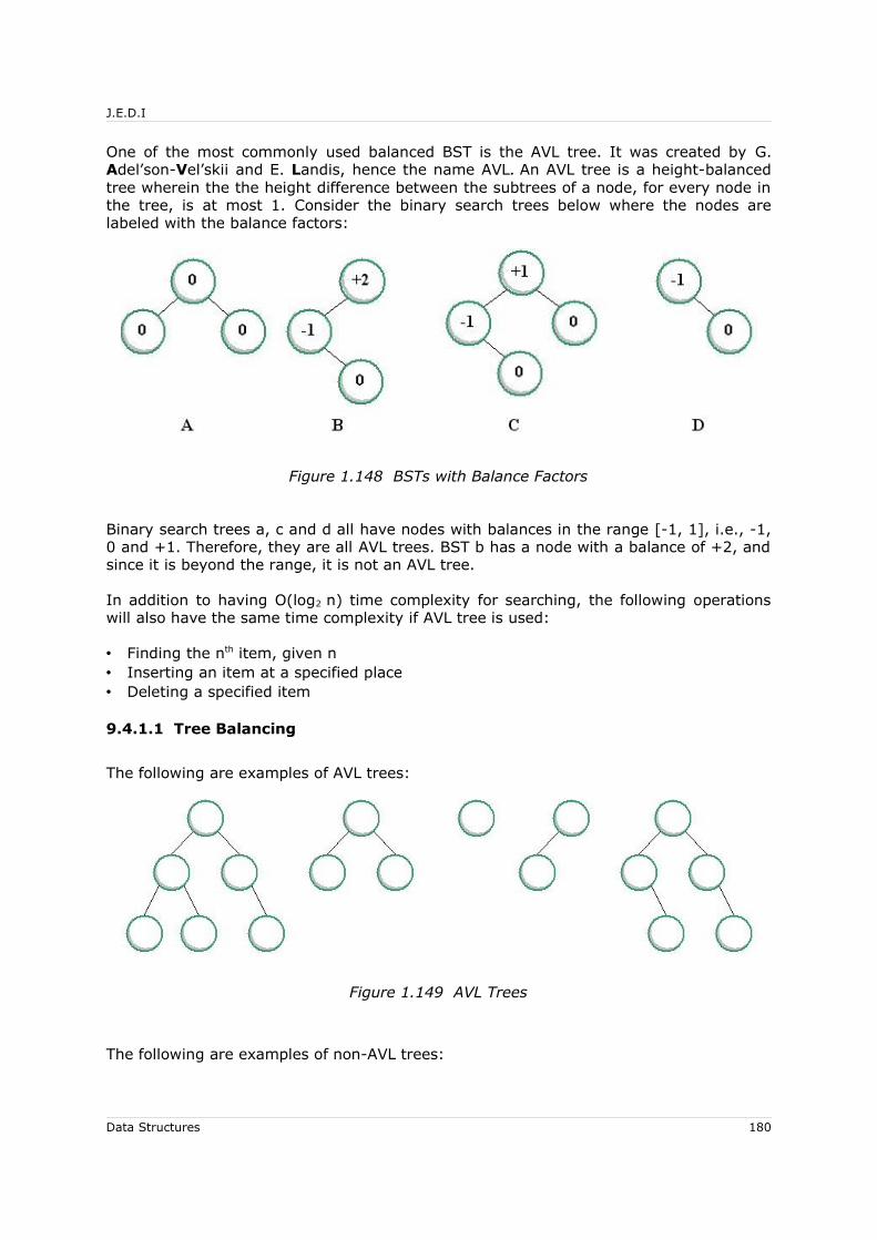
J.E.D.I

One of the most commonly used balanced BST is the AVL tree. It was created by G. Adel’son-Vel’skii and E. Landis, hence the name AVL. An AVL tree is a height-balanced tree wherein the the height difference between the subtrees of a node, for every node in the tree, is at most 1. Consider the binary search trees below where the nodes are labeled with the balance factors:

Figure 1.148 BSTs with Balance Factors

Binary search trees a, c and d all have nodes with balances in the range [-1, 1], i.e., -1, 0 and +1. Therefore, they are all AVL trees. BST b has a node with a balance of +2, and since it is beyond the range, it is not an AVL tree.

In addition to having O(log2 n) time complexity for searching, the following operations will also have the same time complexity if AVL tree is used:

• Finding the nth item, given n• Inserting an item at a specified place• Deleting a specified item

9.4.1.1 Tree Balancing

The following are examples of AVL trees:

Figure 1.149 AVL Trees

The following are examples of non-AVL trees:

Data Structures 180

J.E.D.I

Figure 1.150 Non-AVL Trees

In maintaining the balance of an AVL tree, rotations have to be performed during insertion and deletion. The following are the rotations used:

• Simple right rotation (RR) – used when the new item C is in the left subtree of the left child B of the nearest ancestor A with balance factor +2

Figure 1.151 Simple Right Rotation

Figure 1.152

Figure 1.153

• Simple left rotation (LR) – used when the new item C is in the right subtree of the right child B of the nearest ancestor A with balance factor -2

Figure 1.154 Simple Left Rotation

Data Structures 181

J.E.D.I

Figure 1.155

• Left-right rotation (LRR)– used when the new item C is in the right subtree of the left child B of the nearest ancestor A with balance factor +2

Figure 1.156 Left Right Rotation

• Right-left rotation (RLR) – used when the new item C is in the left subtree of the right child B of the nearest ancestor A with balance factor -2

Figure 1.157 Right Left Rotation

Insertion in an AVL tree is the same as in BST. However, the resulting balance has to be

Data Structures 182

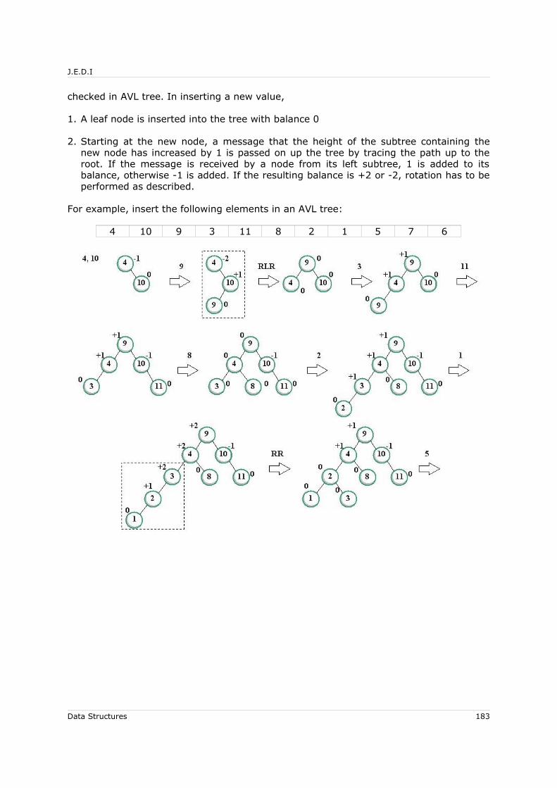
J.E.D.I

checked in AVL tree. In inserting a new value,

1. A leaf node is inserted into the tree with balance 0

2. Starting at the new node, a message that the height of the subtree containing the new node has increased by 1 is passed on up the tree by tracing the path up to the root. If the message is received by a node from its left subtree, 1 is added to its balance, otherwise -1 is added. If the resulting balance is +2 or -2, rotation has to be performed as described.

For example, insert the following elements in an AVL tree:

4 10 9 3 11 8 2 1 5 7 6

Data Structures 183

J.E.D.I

Figure 1.158 Insertion into an AVL Tree

9.5 Summary

• A Binary Search Tree is a binary tree that satisfies the BST property

• Operations on BSTs include insertion of a new key, deletion of an existing key, and searching for a key

• The BST search algorithm runs in O(log2 n) time on the average and O(n)

time on the worst case

• Balanced BSTs ensure that searching takes O(log2 n)

• An AVL tree is a height-balanced tree wherein the height difference between the subtrees of a node for every node in the tree is at most 1

• Rotations have to be performed during insertion and deletion in an AVL tree to maintain its balance

Data Structures 184

J.E.D.I

9.6 Lecture Exercise

1. Insert the following keys in an AVL tree, based on the order given:

a) 1 6 7 4 2 5 8 9 0 3

b) A R F G E Y B X C S T I O P L V


1. Extend the BST class definition to make it an AVL tree, i.e.,

class AVL extends BST{}

Override the insert and delete methods to implement the rotations in an AVL tree to maintain the balance.

Data Structures 185

J.E.D.I

10 Hash Table and Hashing Techniques

10.1 Objectives


• Define hashing and explain how hashing works

• Implement simple hashing techniques

• Discuss how collisions are avoided/minimized by using collision resolution

techniques

• Explain the concepts behind dynamic files and hashing

10.2 Introduction

Hashing is the application of a mathematical function (called a hash function) to the key values that results in mapping the possible range of key values into a smaller range of relative addresses. The hash function is something like a locked box that needs a key to get the output which, in this case, is the address where the key is stored:

key ====> Hash Function H(k) ===> address

With hashing, there is no obvious connection between the key and the address generated since the function "randomly selects" an address for a specific key value, without regard to the physical sequence of the records in the file. Hence, it is also known as randomizing scheme.

Two or more input keys, say k1 and k2, when applied to a hash function, may hash to the same address, an accident known as collision. Collision can be reduced by allocating more file space than the minimum required to store the number of keys. However, this approach leads to wasted space. There are several ways to handle collisions, which will be discussed later.

In hashing, there is a need to choose a good hash function and consequently, select a method to resolve, if not eliminate, collisions. A good hash function performs fast computation, in time complexity of O(1), and produces less (or no) collisions.

Data Structures 186

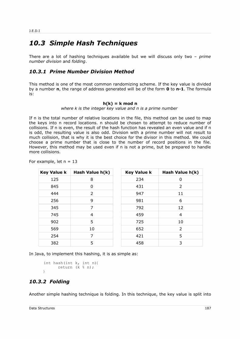
J.E.D.I

10.3 Simple Hash Techniques

There are a lot of hashing techniques available but we will discuss only two – prime number division and folding.

10.3.1 Prime Number Division Method

This method is one of the most common randomizing scheme. If the key value is divided by a number n, the range of address generated will be of the form 0 to n-1. The formula is:

h(k) = k mod nwhere k is the integer key value and n is a prime number

If n is the total number of relative locations in the file, this method can be used to map the keys into n record locations. n should be chosen to attempt to reduce number of collisions. If n is even, the result of the hash function has revealed an even value and if n is odd, the resulting value is also odd. Division with a prime number will not result to much collision, that is why it is the best choice for the divisor in this method. We could choose a prime number that is close to the number of record positions in the file. However, this method may be used even if n is not a prime, but be prepared to handle more collisions.

For example, let n = 13

Key Value k Hash Value h(k) Key Value k Hash Value h(k)

125 8 234 0

845 0 431 2

444 2 947 11

256 9 981 6

345 7 792 12

745 4 459 4

902 5 725 10

569 10 652 2

254 7 421 5

382 5 458 3

In Java, to implement this hashing, it is as simple as:

int hash(int k, int n){return (k % n);

}

10.3.2 Folding

Another simple hashing technique is folding. In this technique, the key value is split into

Data Structures 187

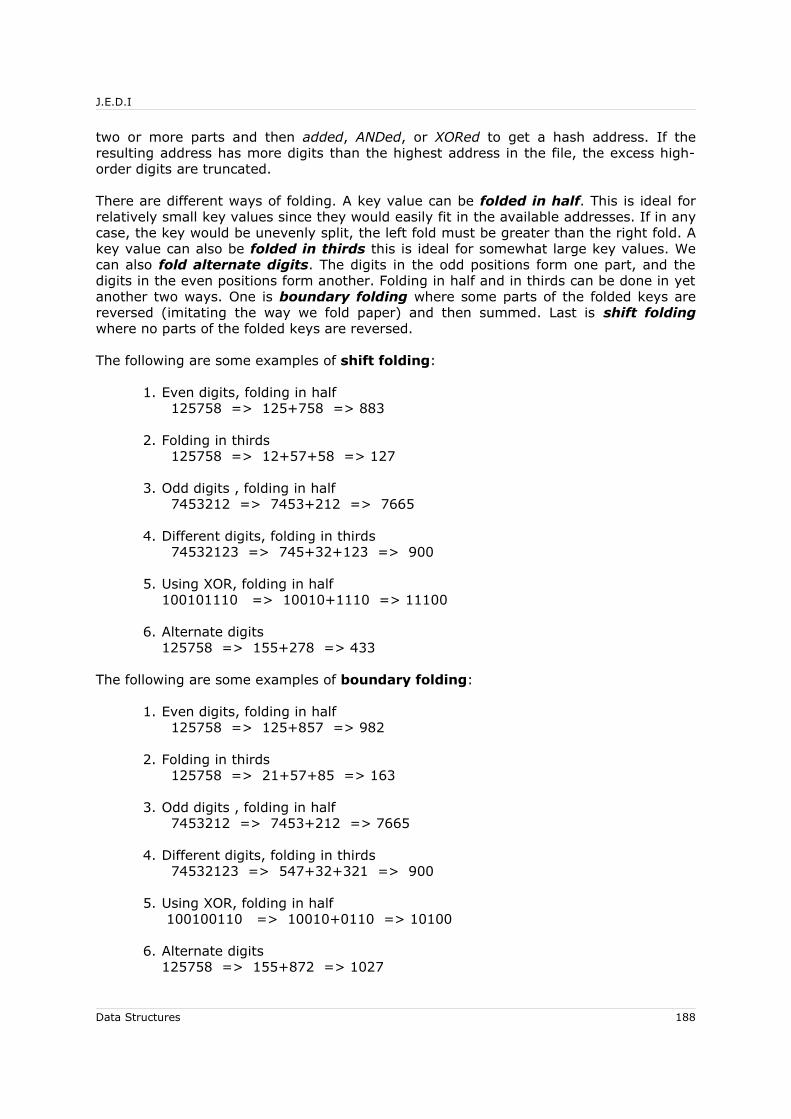
J.E.D.I

two or more parts and then added, ANDed, or XORed to get a hash address. If the resulting address has more digits than the highest address in the file, the excess high-order digits are truncated.

There are different ways of folding. A key value can be folded in half. This is ideal for relatively small key values since they would easily fit in the available addresses. If in any case, the key would be unevenly split, the left fold must be greater than the right fold. A key value can also be folded in thirds this is ideal for somewhat large key values. We can also fold alternate digits. The digits in the odd positions form one part, and the digits in the even positions form another. Folding in half and in thirds can be done in yet another two ways. One is boundary folding where some parts of the folded keys are reversed (imitating the way we fold paper) and then summed. Last is shift folding where no parts of the folded keys are reversed.

The following are some examples of shift folding:

1. Even digits, folding in half 125758 => 125+758 => 883

2. Folding in thirds 125758 => 12+57+58 => 127

3. Odd digits , folding in half 7453212 => 7453+212 => 7665

4. Different digits, folding in thirds 74532123 => 745+32+123 => 900

5. Using XOR, folding in half 100101110 => 10010+1110 => 11100

6. Alternate digits125758 => 155+278 => 433

The following are some examples of boundary folding:

1. Even digits, folding in half 125758 => 125+857 => 982

2. Folding in thirds 125758 => 21+57+85 => 163

3. Odd digits , folding in half 7453212 => 7453+212 => 7665

4. Different digits, folding in thirds 74532123 => 547+32+321 => 900

5. Using XOR, folding in half 100100110 => 10010+0110 => 10100

6. Alternate digits125758 => 155+872 => 1027

Data Structures 188

J.E.D.I

This method is useful for converting keys with large number of digits to a smaller number of digits so the address fits into a word memory. It is also easier to store since the keys do not require much space to be stored.

10.4 Collision Resolution Techniques

Choosing a good hashing algorithm based on how few collisions are likely to occur is the first step in avoiding collision. However, this will just minimize and will not eradicate the problem. To avoid collision, we could:

• spread out records, i.e., finding a hashing algorithm that distributes the records fairly randomly among the available addresses. However, it is hard to find a hashing algorithm that distributes the records evenly.

• use extra memory, if there are memory addresses to distribute the records into, it is easier to find a hashing algorithm than if we have almost equal number of addresses and records. One advantage is that the records are spread out evenly, eventually reducing collisions. However, this method wastes space.

• use buckets, i.e., put more than one record at a single address.

There are several collision resolution techniques and in this section we will cover chaining, use of buckets and open addressing.

10.4.1 Chaining

In chaining, m linked lists are maintained, one for each possible address in the hash table. Using chaining to resolve collision in storing the example in Prime Number Division Method of hashing:


125 8 234 0

845 0 431 2

444 2 947 11

256 9 981 6

345 7 792 12

745 4 459 4

902 5 725 10

569 10 652 2

254 7 421 5

382 5 458 3

We have the following hash table:

Data Structures 189

J.E.D.I

KEY LINK KEY LINK

0 Λ 0 845 234 Λ1 Λ 1 Λ2 Λ 2 444 431 652 Λ3 Λ 3 458 Λ4 Λ 4 745 459 Λ5 Λ 5 902 382 421 Λ6 Λ 6 981 Λ7 Λ 7 345 254 Λ8 Λ 8 125 Λ9 Λ 9 256 Λ

10 Λ 10 569 725 Λ11 Λ 11 947 Λ12 Λ 12 792 Λ

Initial Table After Insertions

Keys 845 and 234 both hash to address 0 so they are linked together in the address. The case is the same for addresses 2, 4, 5, 7 and 10, while the rest of the addresses have no collision. The chaining method resolved the collision by providing additional link nodes to each of the values.

10.4.2 Use of Buckets

Like chaining, this method divides the hash table into m groups of records where each group contains exactly b records, having each address regarded as a bucket.

For example: KEY1 KEY2 KEY3

0 845 234

1

2 444 431 652

3 458

4 745 459

5 902 382 421

6 981

7 345 254

8 125

9 256

10 569 725

11 947

Data Structures 190

J.E.D.I

KEY1 KEY2 KEY3

12 792

Collision is redefined in this approach. It happens when a bucket overflows – that is, when an insertion is attempted on a full bucket. Hence, there is a significant reduction in the number of collisions. However, this method wastes some space and is not free from overflowing further, in which case an overflow policy must be invoked. In the above example, there are three slots in each address. Being static in size, problem arises when more than three values hash to a single address.

10.4.3 Open Addressing (Probing)

In open addressing, when the address produced by a hash function h(k) has no more space for insertion, an empty slot other than h(k) in the hash table is located. This process is called probing. In this empty slot, the new record that has collided with the old one, known as the colliding key, could be safely placed. In this method, we introduce the permutation of the table addresses, say β0, β1, ... βm-1, This permutation is called probe sequence.

In this section, we will cover two techniques: linear probing and double hashing.

10.4.3.1 Linear Probing

Linear probing is one of the simplest techniques in handling collisions in which the file is scanned or probed sequentially as a circular file and the colliding key is stored in the nearest available space to the address. This is used in systems where a “first come, first served” basis is followed. An example is an airline reservation system where seats for chance passengers are given away when passengers for reserved seats don’t arrive. Whenever a collision occurs at a certain address, the succeeding addresses are probed, that is, searched sequentially until an empty one is found. The key then uses this address. Array should be considered circular, so that when the last location is reached, the search proceeds to the first location of the array.

In this method, it is possible that the entire file could be searched, starting at position i+1, and the colliding keys are distributed throughout the file. If a key hashes to position i, which is occupied, positions i+1, …,n are searched for an empty location.

The slots in a hash table may contain only one key or could also be a bucket. In this example, buckets of capacity 2 are used to store the following keys:


125 8 234 0

845 0 431 2

444 2 947 11

256 9 981 6

345 7 792 12

745 4 459 4

Data Structures 191

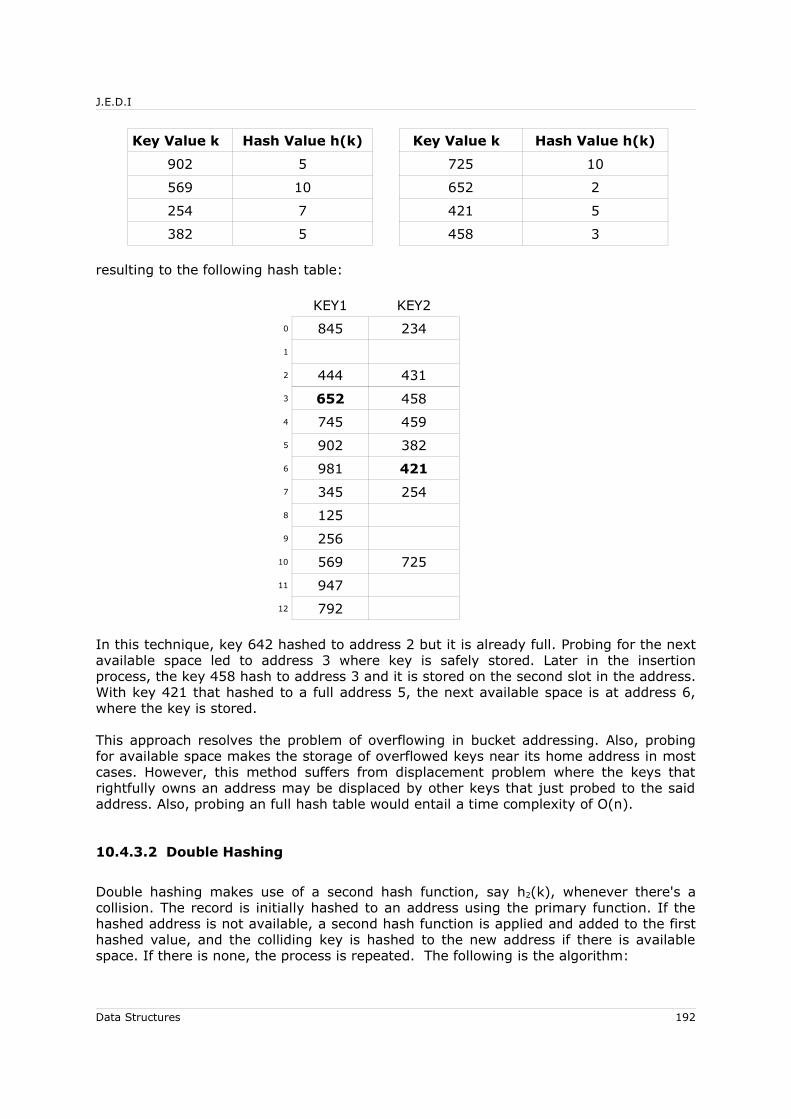
J.E.D.I


902 5 725 10

569 10 652 2

254 7 421 5

382 5 458 3

resulting to the following hash table:

KEY1 KEY2

0 845 234

1

2 444 431

3 652 458

4 745 459

5 902 382

6 981 421

7 345 254

8 125

9 256

10 569 725

11 947

12 792

In this technique, key 642 hashed to address 2 but it is already full. Probing for the next available space led to address 3 where key is safely stored. Later in the insertion process, the key 458 hash to address 3 and it is stored on the second slot in the address. With key 421 that hashed to a full address 5, the next available space is at address 6, where the key is stored.

This approach resolves the problem of overflowing in bucket addressing. Also, probing for available space makes the storage of overflowed keys near its home address in most cases. However, this method suffers from displacement problem where the keys that rightfully owns an address may be displaced by other keys that just probed to the said address. Also, probing an full hash table would entail a time complexity of O(n).

10.4.3.2 Double Hashing

Double hashing makes use of a second hash function, say h2(k), whenever there's a collision. The record is initially hashed to an address using the primary function. If the hashed address is not available, a second hash function is applied and added to the first hashed value, and the colliding key is hashed to the new address if there is available space. If there is none, the process is repeated. The following is the algorithm:

Data Structures 192

J.E.D.I

1. Use the primary hash function h1(k) to determine the position i at which to place the value.

2. If there is a collision, use the rehash function rh(i, k) successively until an empty slot is found:

rh(i, k) = ( i + h2(k)) mod m

where m is the number of addresses

Using the second hash function h2(k)= k mod 11 in storing the following keys:


125 8 234 0

845 0 431 2

444 2 947 11

256 9 981 6

345 7 792 12

745 4 459 4

902 5 725 10

569 10 652 2

254 7 421 5

382 5 458 3

For keys 125, 845, 444, 256, 345, 745, 902, 569, 254, 382, 234, 431, 947, 981, 792, 459 and 725, storage is pretty straightforward – no overflow happened.

KEY1 KEY2

0 845 234

1

2 444 431

3

4 745 459

5 902 382

6 981

7 345 254

8 125

9 256

10 569 725

11 947

12 792

Data Structures 193

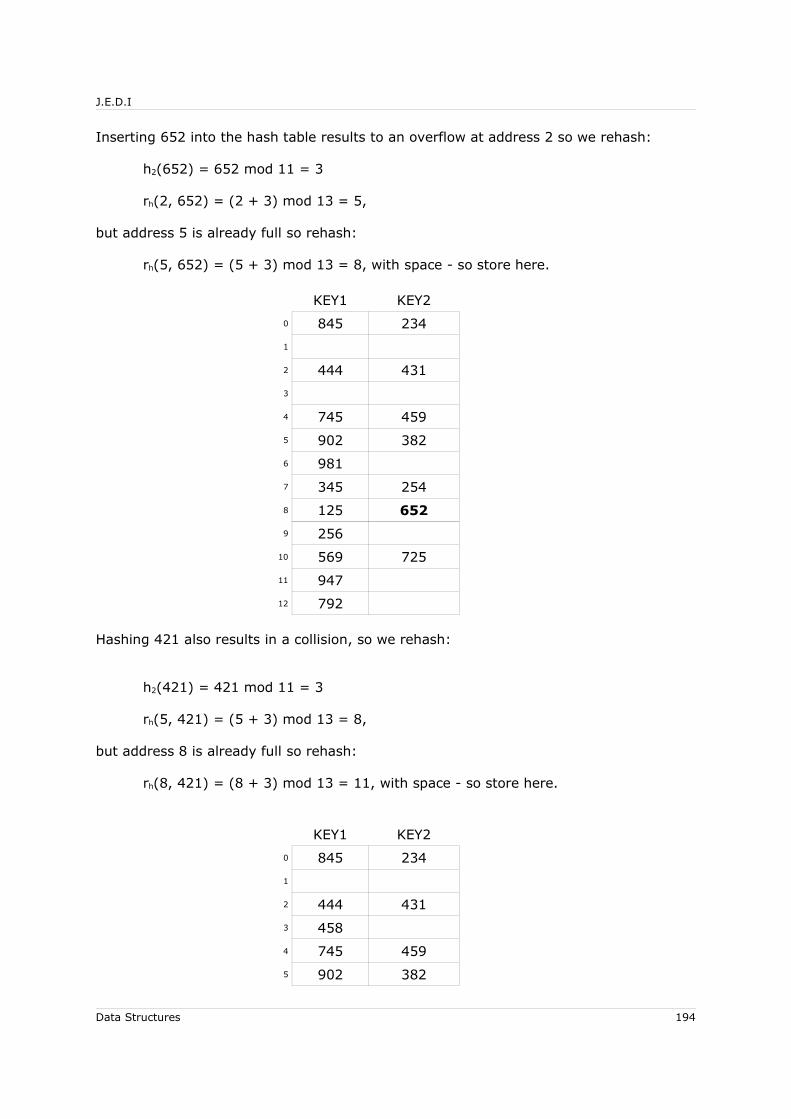
J.E.D.I

Inserting 652 into the hash table results to an overflow at address 2 so we rehash:

h2(652) = 652 mod 11 = 3

rh(2, 652) = (2 + 3) mod 13 = 5,

but address 5 is already full so rehash:

rh(5, 652) = (5 + 3) mod 13 = 8, with space - so store here.

KEY1 KEY2

0 845 234

1

2 444 431

3

4 745 459

5 902 382

6 981

7 345 254

8 125 652

9 256

10 569 725

11 947

12 792

Hashing 421 also results in a collision, so we rehash:

h2(421) = 421 mod 11 = 3

rh(5, 421) = (5 + 3) mod 13 = 8,

but address 8 is already full so rehash:

rh(8, 421) = (8 + 3) mod 13 = 11, with space - so store here.

KEY1 KEY2

0 845 234

1

2 444 431

3 458

4 745 459

5 902 382

Data Structures 194

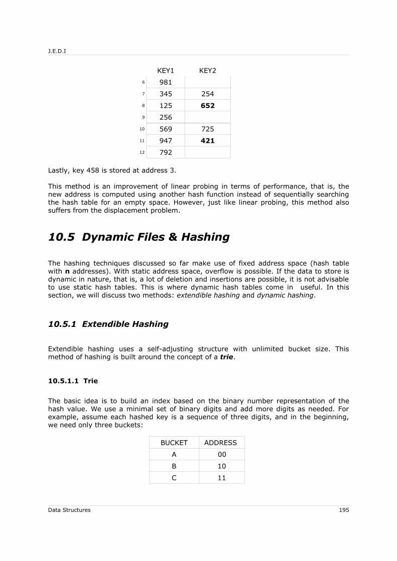
J.E.D.I

KEY1 KEY2

6 981

7 345 254

8 125 652

9 256

10 569 725

11 947 421

12 792

Lastly, key 458 is stored at address 3.

This method is an improvement of linear probing in terms of performance, that is, the new address is computed using another hash function instead of sequentially searching the hash table for an empty space. However, just like linear probing, this method also suffers from the displacement problem.

10.5 Dynamic Files & Hashing

The hashing techniques discussed so far make use of fixed address space (hash table with n addresses). With static address space, overflow is possible. If the data to store is dynamic in nature, that is, a lot of deletion and insertions are possible, it is not advisable to use static hash tables. This is where dynamic hash tables come in useful. In this section, we will discuss two methods: extendible hashing and dynamic hashing.

10.5.1 Extendible Hashing

Extendible hashing uses a self-adjusting structure with unlimited bucket size. This method of hashing is built around the concept of a trie.

10.5.1.1 Trie

The basic idea is to build an index based on the binary number representation of the hash value. We use a minimal set of binary digits and add more digits as needed. For example, assume each hashed key is a sequence of three digits, and in the beginning, we need only three buckets:

BUCKET ADDRESS

A ,00

B 10

C 11

Data Structures 195

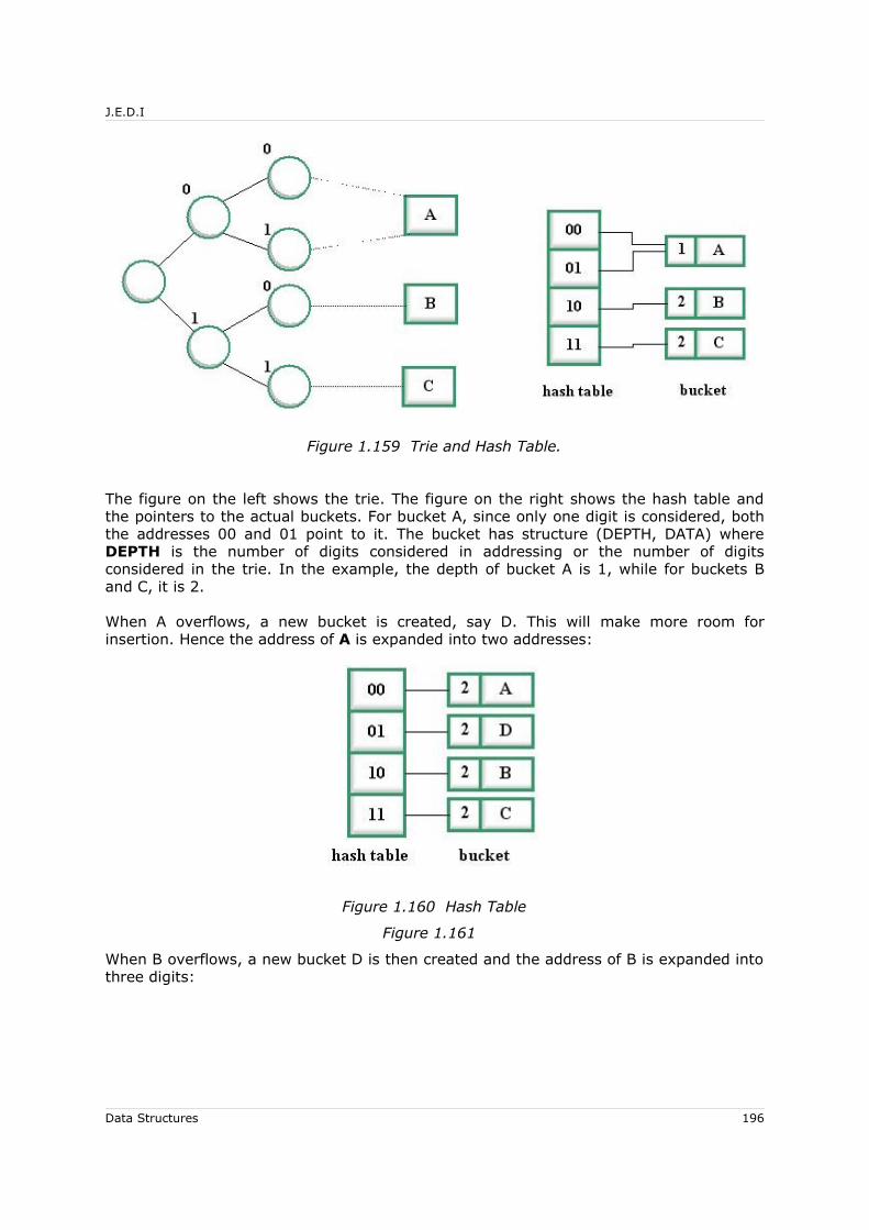
J.E.D.I

Figure 1.159 Trie and Hash Table.

The figure on the left shows the trie. The figure on the right shows the hash table and the pointers to the actual buckets. For bucket A, since only one digit is considered, both the addresses 00 and 01 point to it. The bucket has structure (DEPTH, DATA) where DEPTH is the number of digits considered in addressing or the number of digits considered in the trie. In the example, the depth of bucket A is 1, while for buckets B and C, it is 2.

When A overflows, a new bucket is created, say D. This will make more room for insertion. Hence the address of A is expanded into two addresses:

Figure 1.160 Hash Table

Figure 1.161

When B overflows, a new bucket D is then created and the address of B is expanded into three digits:

Data Structures 196

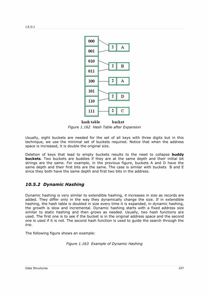
J.E.D.I

Figure 1.162 Hash Table after Expansion

Usually, eight buckets are needed for the set of all keys with three digits but in this technique, we use the minimal set of buckets required. Notice that when the address space is increased, it is double the original size.

Deletion of keys that lead to empty buckets results to the need to collapse buddy buckets. Two buckets are buddies if they are at the same depth and their initial bit strings are the same. For example, in the previous figure, buckets A and D have the same depth and their first bits are the same. The case is similar with buckets B and E since they both have the same depth and first two bits in the address.

10.5.2 Dynamic Hashing

Dynamic hashing is very similar to extendible hashing, it increases in size as records are added. They differ only in the way they dynamically change the size. If in extendible hashing, the hash table is doubled in size every time it is expanded, in dynamic hashing, the growth is slow and incremental. Dynamic hashing starts with a fixed address size similar to static hashing and then grows as needed. Usually, two hash functions are used. The first one is to see if the bucket is in the original address space and the second one is used if it is not. The second hash function is used to guide the search through the trie.

The following figure shows an example:

Figure 1.163 Example of Dynamic Hashing

Data Structures 197

J.E.D.I

The example shows the original address space consisting of four addresses. An overflow at address 4 results to its expansion into using two digits 40 and 41. There is also an overflow at address 2, so it is expanded into 20 and 21. An overflow at address 41 resulted into using three digits 410 and 411.

10.6 Summary• Hashing maps the possible range of key values into a smaller range of relative

addresses.• Simple hash techniques include the prime number division method and folding.• Chaining makes use of m linked lists, one for each possible address in the hash

table.• In the use of buckets method, collision happens when a bucket overflows.• Linear probing and double hashing are two open addressing techniques.• Dynamic hash tables are useful if data to be stored is dynamic in nature. Two

dynamic hashing techniques are extendible hashing and dynamic hashing.•

Data Structures 198

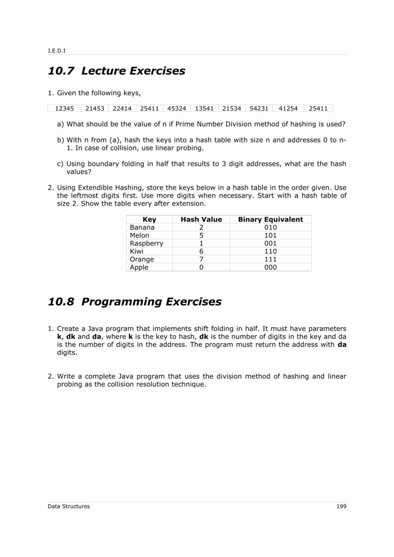
J.E.D.I


1. Given the following keys,

12345 21453 22414 25411 45324 13541 21534 54231 41254 25411

a) What should be the value of n if Prime Number Division method of hashing is used?

b) With n from (a), hash the keys into a hash table with size n and addresses 0 to n-1. In case of collision, use linear probing.

c) Using boundary folding in half that results to 3 digit addresses, what are the hash values?

2. Using Extendible Hashing, store the keys below in a hash table in the order given. Use the leftmost digits first. Use more digits when necessary. Start with a hash table of size 2. Show the table every after extension.

Key Hash Value Binary EquivalentBanana 2 010Melon 5 101Raspberry 1 001Kiwi 6 110Orange 7 111Apple 0 000


1. Create a Java program that implements shift folding in half. It must have parameters k, dk and da, where k is the key to hash, dk is the number of digits in the key and da is the number of digits in the address. The program must return the address with da digits.

2. Write a complete Java program that uses the division method of hashing and linear probing as the collision resolution technique.

Data Structures 199

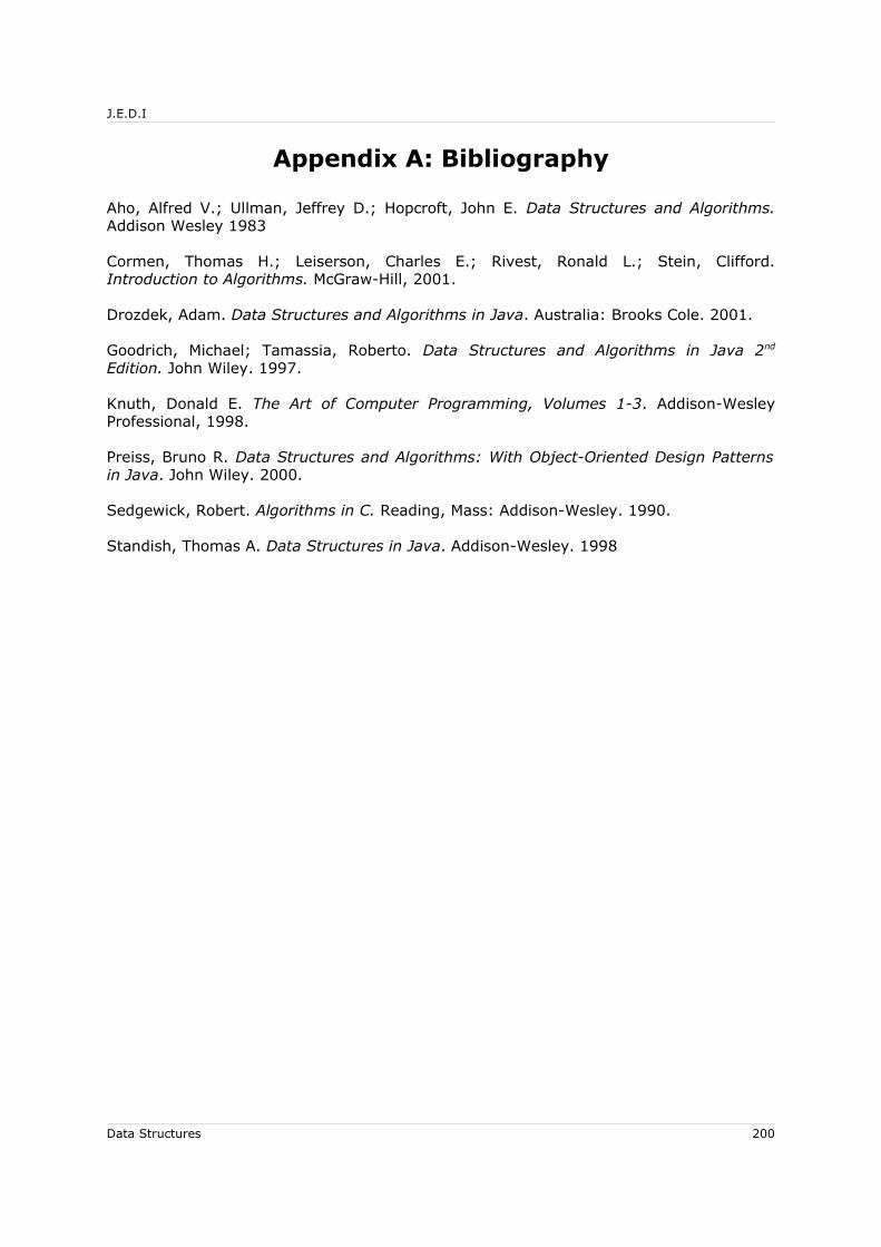
J.E.D.I

Appendix A: Bibliography

Aho, Alfred V.; Ullman, Jeffrey D.; Hopcroft, John E. Data Structures and Algorithms. Addison Wesley 1983

Cormen, Thomas H.; Leiserson, Charles E.; Rivest, Ronald L.; Stein, Clifford. Introduction to Algorithms. McGraw-Hill, 2001.

Drozdek, Adam. Data Structures and Algorithms in Java. Australia: Brooks Cole. 2001.

Goodrich, Michael; Tamassia, Roberto. Data Structures and Algorithms in Java 2nd

Edition. John Wiley. 1997.

Knuth, Donald E. The Art of Computer Programming, Volumes 1-3. Addison-Wesley Professional, 1998.

Preiss, Bruno R. Data Structures and Algorithms: With Object-Oriented Design Patterns in Java. John Wiley. 2000.

Sedgewick, Robert. Algorithms in C. Reading, Mass: Addison-Wesley. 1990.

Standish, Thomas A. Data Structures in Java. Addison-Wesley. 1998

Data Structures 200

Data Structures - Komputasi · PDF fileJ.E.D.I Author Joyce Avestro Team Joyce Avestro...

Documents

Transcript of Data Structures - Komputasi · PDF fileJ.E.D.I Author Joyce Avestro Team Joyce Avestro...