Data sparse approximation of the Karhunen-Loeve expansion

Data sparse approximation of theKarhunen-Loeve expansion

A. Litvinenko, joint work with B. Khoromskij and H. G. Matthies

Institut fur Wissenschaftliches Rechnen, Technische Universitat Braunschweig,0531-391-3008, [email protected]

December 5, 2008

Outline

Introduction

KLE

Hierarchical Matrices

Low Kronecker rank approximation

Application

Stochastic PDE

We consider

− div(κ(x , ω)∇u) = f (x , ω) in G,u = 0 on ∂G,

with stochastic coefficients κ(x , ω), x ∈ G ⊆ Rd and ω belongs to the

space of random events Ω.

Figure: Examples of computational domains G with a non-rectangular grid.

Covariance functions

The random field f (x , ω) requires to specify its spatial correl. structure

covf (x , y) = E[(f (x , ·) − µf (x))(f (y , ·) − µf (y))],

Let h =

√∑3i=1 h2

i /ℓ2i , where hi := xi − yi , i = 1, 2, 3, ℓi are cov.

lengths.

Examples: Gaussian cov(h) = exp(−h2), exponentialcov(h) = exp(−h),

Outline

Introduction

KLE



Application

KLE

The Karhunen-Loeve expansion is the series

κ(x , ω) = µk (x) +

∞∑

i=1

√λiφi (x)ξi(ω), where

ξi (ω) are uncorrelated random variables and φi are basis functions inL2(G).Eigenpairs λi , φi are the solution of

Tφi = λiφi , φi ∈ L2(G), i ∈ N, where.

T : L2(G) → L2(G),(Tφ)(x) :=

∫G covk (x , y)φ(y)dy .

Discrete eigenvalue problem

Let

Wij :=∑

k ,m

∫

G

bi(x)bk (x)dxCkm

∫

G

bj (y)bm(y)dy ,

Mij =

∫

G

bi(x)bj(x)dx .

Then we solve

Wφhℓ = λℓMφh

ℓ , where W := MCM

Approximate C and M in

the H-matrix format low Kronecker rank format

and use the Lanczos method to compute m largest eigenvalues.

Outline

Introduction

KLE



Application

Examples of H-matrix approximates ofcov(x , y) = e−2|x−y |

25 20

20 20

20 16

20 16

20 20

16 16

20 16

16 16

4 4

20 4 324 4

16 4 324 20

4 4

4 16

4 4

32 32

20 20

20 20 32

32 32

4 3

4 4 3220 4

16 4 32

32 4

32 32

4 32

32 32

32 4

32 324 4

4 4

20 16

4 4

32 32

4 32

32 32

32 32

4 32

32 32

4 32

20 20

20 20 32

32 32

32 32

32 32

32 32

32 32

32 32

32 32

4 44 4

20 4 32

32 32 4

4 432 4

32 32 4

4 432 32

4 32 4

4 432 32

32 32 4

44 20

4 4 32

32 32

4 4

432 4

32 32

4 4

432 32

4 32

4 4

432 32

32 32

4 4

20 20

20 20 32

32 32

4 4

20 4 32

32 324 20

4 4 32

32 32

20 20

20 20 32

32 32

32 4

32 32

32 4

32 32

32 4

32 32

32 4

32 32

32 32

4 32

32 32

4 32

32 32

4 32

32 32

4 32

32 32

32 32

32 32

32 32

32 32

32 32

32 32

32 32

4 4

4 4 44 4

20 4 32

32 32

32 4

32 32

4 32

32 32

32 4

32 32

4 4

4 4

4 4

4 4 44 4

32 4

32 32 4

4 4

4 4

4 4

4 4 44

32 4

32 32

4 4

4 4

4 4

4 4

4 4 432 4

32 32

32 4

32 32

32 4

32 32

32 4

32 32

4 4

4 4

4 4

4 4

4 20

4 4 32

32 32

4 32

32 32

32 32

4 32

32 32

4 32

44 4

4 4

4 4

4 4

4 432 32

4 32 4

44 3

4 4

4 4

4 4

432 32

4 32

4 4

44 4

4 4

4 4

4 4

32 32

4 32

32 32

4 32

32 32

4 32

32 32

4 32

44 4

4 4

20 20

20 20 32

32 32

32 32

32 32

32 32

32 32

32 32

32 32

4 4

20 4 32

32 32

32 4

32 32

4 32

32 32

32 4

32 324 20

4 4 32

32 32

4 32

32 32

32 32

4 32

32 32

4 32

20 20

20 20 32

32 32

32 32

32 32

32 32

32 32

32 32

32 32

4 432 32

32 32 4

4 432 4

32 32 4

4 432 32

4 32 4

4 432 32

32 32 4

432 32

32 32

4 4

432 4

32 32

4 4

432 32

4 32

4 4

432 32

32 32

4 4

32 32

32 32

32 32

32 32

32 32

32 32

32 32

32 32

32 4

32 32

32 4

32 4

32 4

32 32

32 4

32 4

32 32

4 32

32 32

4 32

32 32

4 4

32 32

4 4

32 32

32 32

32 32

32 32

32 32

32 32

32 32

32 32

25 11

11 20 12

1320 11

9 1613

1320 11

11 20 13

13 3213

13

20 8

10 20 13

13 32 13

1332 13

13 32

13

13

20 11

11 20 13

13 32 13

1320 10

10 20 12

12 3213

1332 13

13 32 13

1332 13

13 32

13

13

20 11

11 20 13

13 32 13

1332 13

13 3213

13

20 9

9 20 13

13 32 13

1332 13

13 32

13

13

32 13

13 32 13

1332 13

13 3213

1332 13

13 32 13

1332 13

13 32

Figure: H-matrix approximations C ∈ Rn×n, n = 322, with standard (left) and

weak (right) admissibility block partitionings. The biggest dense (dark) blocks∈ R

n×n, max. rank k = 4 left and k = 13 right.

H - matrices: numerics

To assemble low-rank blocks use ACA [Bebendorf et al. ].

Dependence of the computational time and storage requirements ofC on the rank k , n = 322.

k time (sec.) memory (MB) ‖C−C‖2

‖C‖2

2 0.04 2 3.5e − 56 0.1 4 1.4e − 59 0.14 5.4 1.4e − 512 0.17 6.8 3.1e − 717 0.23 9.3 6.3e − 8

The time for dense matrix C is 3.3 sec. and the storage 140 MB.


k size, MB t , sec.1 1548 332 1865 423 2181 504 2497 596 nem -

k size, MB t , sec.4 463 118 850 2212 1236 3216 1623 4320 nem -

Table: Computing times and storage requirements on the H-matrix rank k forthe exp. cov. function. (left) standard admissibility condition, geometryshown in Fig. 1 (middle), l1 = 0.1, l2 = 0.5, n = 2.3 · 105. (right) weakadmissibility condition, geometry shown in Fig. 1 (right), l1 = 0.1, l2 = 0.5,l3 = 0.1, n = 4.61 · 105.


k 2.4 · 104 3.5 · 104 6.8 · 104 2.3 · 105

t1 t2 t1 t2 t1 t2 t1 t23 3 · 10−3 0.2 6.0 · 10−3 0.4 1 · 10−2 1 5.0 · 10−2 46 6 · 10−3 0.4 1.1 · 10−2 0.7 2 · 10−2 2 9.0 · 10−2 79 8 · 10−3 0.5 1.5 · 10−2 1.0 3 · 10−2 3 1.3 · 10−1 11

full 0.62 2.48 10 140

Table: t1- computing times (in sec.) required for an H-matrix and densematrix vector multiplication, t2 - times to set up C ∈ R

n×n.


exponential cov(h) = exp(−h),The cov. matrix C ∈ R

n×n, n = 652.

ℓ1 ℓ2‖C−C‖2

‖C‖2

0.01 0.02 3 · 10−2

0.1 0.2 8 · 10−3

1 2 2.8 · 10−6

m - eigenvalues

matrix info (MB, sec.) mn k C, MB C, sec. 2 5 10 20 40 80

2.4 · 104 4 12 0.2 0.6 0.9 1.3 2.3 4.2 86.8 · 104 8 95 2 2.4 3.8 5.6 8.4 18.0 282.3 · 105 12 570 11 10.0 17.0 24.0 39.0 70.0 150

Table: Time required for computing m eigenpairs of the exp. cov. functionwith l1 = l3 = 0.1, l3 = 0.5. The geometry is shown in Fig. 1 (right).

Outline

Introduction

KLE



Application

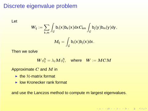
Sparse tensor decompositions of kernelscov(x , y) = cov(x − y)

We want to approximate C ∈ RN×N , N = nd by

Cr =

r∑

k=1

V 1k ⊗ ... ⊗ V d

k

such that ‖C − Cr‖ ≤ ε. The storage of C is O(N2) = O(n2d ) and the

storage of Cr is O(rdn2).

To define V ik use SVD.

Approximate all V ik in the H-matrix format ⇒ HKT format.

See basic arithmetics in [Hackbusch, Khoromskij, Tyrtyshnikov].

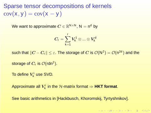
Tensor approximation

Wφhℓ = λℓMφh

ℓ , where W := MCM .

Approximate

M ≈d∑

ν=1

M (1)ν ⊗ M (2)

ν , C ≈q∑

ν=1

C(1)ν ⊗ C(2)

ν , φ ≈r∑

ν=1

φ(1)ν ⊗ φ(2)

ν ,

where M(j)ν , C

(j)ν ∈ R

n×n, φ(j)ν ∈ R

n,Example: for mass matrix M ∈ R

N×N holds

M = M (1) ⊗ I + I ⊗ M (1), where M (1) ∈ Rn×n

is one-dimensional mass matrix.Hypothesis: the Kronecker rank of M stays small even for a moregeneral domain with non-regular grid.

Suppose C =∑q

ν=1 C(1)ν ⊗ C

(2)ν and φ =

∑rj=1 φ

(1)j ⊗ φ

(2)j . Then

tensor vector product is defined as

Cφ =

q∑

ν=1

r∑

j=1

(C(1)ν φ

(1)j ) ⊗ (C(2)

ν φ(2)j ).

The complexity is O(qrkn log n).

Numerical examples of tensor approximations

Gaussian kernel exp(−h2) has the Kroneker rank 1.

The exponen. kernel exp(−h) can be approximated by a tensor withlow Kroneker rank

r 1 2 3 4 5 6 10‖C−Cr‖∞

‖C‖∞

11.5 1.7 0.4 0.14 0.035 0.007 2.8e − 8‖C−Cr‖2

‖C‖26.7 0.52 0.1 0.03 0.008 0.001 5.3e − 9

Example

Let G = [0, 1]2, Lh the stiffness matrix computed with the five-pointformula. Then ‖Lh‖2 ≤ 8h−2 cos2(πh/2) < 8h−2.

LemmaThe (n − 1)2 eigenvectors of Lh are uνµ (1 ≤ ν, µ ≤ n − 1):

uνµ(x , y) = sin(νπx) sin(µπy), (x , y) ∈ Gh.

The corresponding eigenvalues are

λνµ = 4h−2(sin2(νπh/2) + sin2(µπh/2)), 1 ≤ ν, µ ≤ n − 1.

Use Lanczos method with the matrix in the HKT format to computeeigenpairs of

Lhvi = λivi , i = 1..N.

Then we compare the computed eigenpairs with the analyticallyknown eigenpairs.

Outline

Introduction

KLE



Application

Higher order moments

Let operator K be deterministic and

Ku(θ) =∑

α∈J

Ku(α)Hα(θ) = f(θ) =∑

α∈J

f (α)Hα(θ), with

u(α) = [u(α)1 , ..., u(α)

N ]T . Projecting onto each Hα obtain

Ku(α) = f (α).

The KLE of f(θ) is

f(θ) = f +∑

ℓ

√λℓφℓ(θ)fℓ =

∑

ℓ

∑

α

√λℓφ

(α)ℓ Hα(θ)fℓ

=∑

α

Hα(θ)f (α),

where f (α) =∑

ℓ

√λℓφ

(α)ℓ fℓ.

The 3-rd moment of u is

M(3)u = E

∑

α,β,γ

u(α) ⊗ u(β) ⊗ u(γ)HαHβHγ

=∑

α,β,γ

u(α)⊗u(β)⊗u(γ)cα,β,γ ,

cα,β,γ := E (Hα(θ)Hβ(θ)Hγ(θ)) = c(γ)α,β · γ!, and

c(γ)α,β :=

α!β!

(g − α)!(g − β)!(g − γ)!, g := (α + β + γ)/2.

Using u(α) = K−1f (α) =∑

ℓ

√λℓφ

(α)ℓ K−1fℓ and uℓ := K−1fℓ,

obtainM

(3)u =

∑

p,q,r

tp,q,r up ⊗ uq ⊗ ur , where

tp,q,r :=√

λpλqλr

∑

α,β,γ

φ(α)p φ

(β)q φ

(γ)r cα,β,γ .

Literature

1. B.N. Khoromskij, A.Litvinenko, H. G. Matthies, Application ofhierarchical matrices for computing the Karhunen-Loeveexpansion, Computing, 2008, Springer Wien,http://dx.doi.org/10.1007/s00607-008-0018-3

2. B.N. Khoromskij, A.Litvinenko, Data Sparse Computation of theKarhunen-Loeve Expansion, 2008, AIP Conference Proceedings,1048-1, pp. 311-314.

3. H. G. Matthies, Uncertainty Quantification with Stochastic FiniteElements, Encyclopedia of Computational Mechanics, Wiley,2007.

4. W. Hackbusch, B. N. Khoromskij, S. A. Sauter, and E. E.Tyrtyshnikov, Use of Tensor Formats in Elliptic EigenvalueProblems, Preprint 78/2008, MPI for mathematics in Leipzig.

Thank you for your attention!

Questions?

Data sparse approximation of the Karhunen-Loeve expansion

Education

Transcript of Data sparse approximation of the Karhunen-Loeve expansion