Data Resilience Via Data Aggregation: OvercomingOverall Storage Overflow in Sensor Networks

Abstract—Data resilience refers to the ability of long-termviability and availability of data despite insufficiencies of (ordisruptions to) the physical infrastructure that stores the data.In this paper, we identify, formulate, and solve a data resilienceproblem that uniquely arises from sensor networks operating inan inaccessible or inhospitable region, or under extreme weather.In these challenging environments, it is not feasible to install along-term base station in the field. Data generated must be storedinside the network for some period of time before uploadingopportunities become available. Consequently, the collected datacould soon overflow the storage capacity available in the entirenetwork, making discarding valuable data inevitable. We refer tothis data disruption as overall storage overflow in sensor networks.To overcome this obstacle, we propose data resilience via dataaggregation problem (DRA), which employs data aggregationtechniques to reduce the overflow data size so that they canfit into the storage in the network. The goal of DRA is tominimize the total energy consumption during this process whilepreserving as much information as possible. Our work is thefirst one to employ data aggregation to achieve data resilienceagainst overall storage overflow problem in sensor networks.We show that solving DRA is equivalent to solving a multipletraveling salesman walk problem (MTSW) in an appropriatelytransformed graph of the sensor network. We prove that MTSWis NP-hard. We then solve it optimally in linear topologies, anddesign a (2 − 1

q)-approximation algorithm for general graph

topologies, where q is number of nodes to visit. We design aheuristic algorithm to further improve upon the approximationalgorithm, and empirically show that it constantly outperformsthe approximation algorithm by 20%− 30%, in terms of energyconsumption, under different network parameters.

Keywords – Data Resilience, Data Aggregation, OverallStorage Overflow, Sensor Networks, Energy-Efficiency

I. Introduction

Background and Motivation. Data resilience refers to theability of a network storing the data to recover quicklyand to continue maintaining availability of data despite ofany disruptions (such as equipment failure, power outage, oreven malicious attack). Due to resource constraints of sensornetworks such as unreplenishable battery power and limitedstorage capacity of sensor nodes [10, 11], link unreliabilityand scarce bandwidth of wireless medium [45], and the in-hospitable and harsh environments in which they are deployed[5], sensor nodes are often prone to failure and vulnerableof data loss. Therefore, how to ensure that data collected atsensor nodes reach the base station reliably despite all thevulnerabilities has been an active research topic since theinception of sensor network research. This line of researchare usually named under the umbrella of data resilience [10,11], data persistence [2, 24], or reliable data transmission [9].We use data resilience throughout the paper.

Meanwhile, with the advance in sensor technology and ma-turity of sensor network design and deployment, scientists areready to utilize sensor networks to explore the physical worldin a scope and a depth that was never reached before, and tosolve some of the most fundamental problems facing humanbeings. These fundamental problems include disaster warning,climate change, and renewable energy. The emerging sensornetworks designed for those scientific applications includeseismic sensor networks [39], underwater or ocean sensornetworks [17], wind and solar harvesting [16, 31], and volcanoeruption monitoring and glacial melting monitoring [29, 40].One common characteristic of these sensor networks is thatthey are all deployed in challenging environments such as inremote or inhospitable regions, or under extreme weather, tocontinuously collect large volumes of data for a long periodof time without much human intervention. Consequently, it isnot practical to deploy data-collecting base stations with poweroutlets in or near such inaccessible sensor fields. Thereuponsensory data generated in such environments have to be storedinside the network for some period of time and then beingcollected by periodic visits of robots or data mules [15], orby low rate satellite link [30]. Due to the lack of humanintervention and the inadequacy of maintenance in the inhos-pitable environments, such sensor networks must operate muchmore resiliently than the traditional sensor networks (with basestations and in friendly environments).

Data Resilience Against Storage Overflow Disruption. Inthis paper, we focus on data resilience against sensor storageoverflow, wherein storage spaces of some sensor nodes aredepleted and therefore it can not store any newly generateddata. Storage overflow is a major obstacle existing in aboveemerging networks, due to the following reasons. On oneside, massive amounts of data in above scientific applicationsare generated, sensing a wide range of physical properties inreal world ranging from solar light to wind flow to seismicactivity. On the other side, storage is still a serious resourceconstraint of sensor nodes, despite the advances in energy-efficient flash storage [32] with good compression algorithms(data is compressed before stored) and good aging algorithms(fidelity of older data is reduced to make space for newerdata). As a consequence, the massive sensory data couldsoon overflow data storage of sensor nodes and causes dataloss. From scientific perspective, data are “first class citizens”because every bit of data could potentially be important forscientists to analyze the physical world. Thus how to resilientlymaintain such overflow data inside the network and prevent

2

data loss becomes a crucial task. Below we outline two levelsof data overflow disruptions, and provide corresponding dataresilience measures.• Node Storage Overflow. Some sensor nodes are close to

the events of interest and are constantly generating sensorydata, depleting their own storages and causing data loss.We refer to such disruption as node storage overflow, andthe sensor nodes with depleted storage spaces while stillgenerating data as data nodes. The newly generated datathat can no longer be stored at data nodes is called overflowdata. The resilience measure to avoid such data loss issimple: the overflow data is offloaded to other nodes withavailable storages (referred to as storage nodes).1 Differentdata offloading techniques have been proposed with the goalsof either minimizing the total energy consumption duringdata offloading [35], or maximizing the minimum remainingenergy of storage nodes to prolong network lifetime[14], oroffloading the the most useful information considering datacould have different priorities [43].• Overall Storage Overflow. However, data offloading can

not help when the total size of the overflow data is largerthan the total size of the available storage in the network. Werefer to this disruption as overall storage overflow in sensornetworks, wherein discarding data becomes inevitable if noactions taken. This is obviously a more severe disruptioncompared to the storage flow of individual nodes. For thelarge amount of overflow data generated in the sensornetworks, how to guarantee that as much useful informationas possible can be maintained while being fitted into theavailable storage of the network becomes a new challenge.In this paper, we endeavor to answer following question:For sensor networks operating in challenging environmentswhere base station is absent and human intervention impos-sible, how to retain all the information notwithstanding theoverall storage overflow?

Data Aggregation. Fortunately, due to spatial correlation thatcommonly exist among sensory data collected from sensornetworks, we can employ data aggregation techniques toreduce data size. We formulate a graph-theoretic problemcalled data resiliency via data aggregation (DRA), and solveit by designing a suite of new data aggregation algorithmsto aggregate overflow data, so that they can fit into theavailable storage in the network. Our goal is to minimize totalenergy consumption during data aggregation, since batterypower of sensor nodes is still one of the most stringentresources in sensor networks and data aggregation, beingwireless communication, costs most of the battery power. Afterbeing aggregated to the size accommodable by the availablestorage capacity, the overflow data can then be offloaded tostorage nodes using techniques proposed in [14, 35, 43].

Difference Between Data Aggregation in DRA and TraditionalData Aggregation. Data aggregation in DRA is significantly

1Sensor nodes that generate data but have not depleted their storage areconsidered as storage nodes, since they can store overflow data from others.

different from traditional data aggregation in sensor networks[19, 22, 25, 34, 36, 41, 42] in both goals and techniques.• In traditional sensor networks (with base stations), dataaggregation is to combine the data from different sourcesen route to the base station, by eliminating redundancyand reducing the total number of transmissions, thus savingenergy. The goal of data aggregation in DRA, however, is toaggregate the overflow data so that they can fit into availablestorage, therefore preventing data loss caused by overallstorage overflow. It therefore calls for new data aggregationtechniques that not only reduce the size of sensory datawhile sacrificing no information loss, but also guarantee thataggregated data can be stored inside the network.• Unlike most of the existing data aggregation techniques[19, 22, 25, 41, 42] wherein the underlying routing structuresare trees rooted at base station covering all sensor nodes,at the core of the DRA is a novel routing structure calledq-edge forest, which is a graph with q edges and with eachconnected component a tree. Here q is number of datanodes that aggregate their overflow data. Algorithmically,DRA encapsulates a new graph-theoretic problem calledmultiple traveling salesman walks (MTSW), which has notbeen studied before.

Contributions of This Paper. The main contributions of thispaper include the following:1). We identify, formulate, and solve DRA, the data resilienceproblem via data aggregation, to address overall storageoverflow in sensor networks. (Section II

2), We show that DRA in sensor network is equivalent to anew multiple traveling salesman walk problem (MTSW) ina graph appropriately transformed from the sensor networkgraph. (Section IV)

3). We show that the MTSW is NP-hard, by showing that itgeneralizes traveling salesman walk problem [20], which isNP-hard. (Section III-A)

4). We solve optimally the MTSW in linear topologies,and design a (2 − 1

q )-approximation algorithm for generalgraph topologies, where q is number of nodes to visit.(Section III-B)

5). We design a heuristic algorithm to further improve uponthe approximation algorithm, and empirically shows that itoutperforms the approximation algorithm by 10% − 20%,in terms of energy consumption, under different networkparameters. (Section V)

II. Data Resilience Via Data Aggregation Problem (DRA)

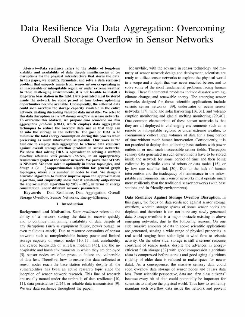
Problem Statement. In a sensor network field (without basestations), there are two kinds of sensor nodes: data nodes(with overflow data and with storage spaces depleted), andstorage nodes (with available storage spaces), as shown inFigure 1. The total size of the overflow data from data nodesis larger than the total size of the storage space availableat storage nodes, causing overall storage overflow. Thereforeoverflow data needs to be aggregated to the size that can fitinto the available storages, before being offloaded to storage

3

Fig. 1. An illustration of DRA.

nodes. To aggregate data, one (or multiple) data node (calledan initiator) sends its overflow data to other data nodes.When a data node (called an aggregators) receives the data,it aggregates its own overflow data to reduce its size. Afterthat, the aggregator forwards initiators’ data to “visit” anotherdata node, which then becomes an aggregator and aggregatesits overflow data, and so on and so forth. This continues untilenough aggregators are visited such that the total size of thedata at data nodes after aggregation equals to or is slightlyless than the total available storage in the network. A storagenode can not be an aggregator since it does not have overflowdata – when it receives the data, it simply relays it.

Any node participating in this process (including initiator,aggregator, and relaying storage node) consumes its ownbattery energy. To save energy consumption, the challenge istherefore to select initiators among all the data nodes, andto decide the sequence of aggregators/storage nodes to visitby each initiator, such that enough number of aggregators arevisited while incurring minimum total energy consumption.

Network Model. The sensor network is represented asan undirected connected graph G(V,E), where V ={1, 2, ..., |V |} is the set of |V | uniformly deployed sensornodes, and E is the set of |E| edges. Two sensor nodes areconnected by an edge if they are within transmission rangeof each other and thus can communicate directly (we assumethat all the nodes have the same transmission range). Thereare p data nodes, denoted as Vd (the other |V | − p nodes arestorage nodes). Let R denote the size of generated overflowdata in bits at each data node and let m be the availablestorage space in bits at each storage node (our work can beextended to the cases wherein data nodes have different sizesof overflow data and/or storage nodes have different sizes ofstorage spaces). Due to the overall storage overflow, we havep×R > (|V | − p)×m, giving that p > |V |m

m+R and p ∈ Z+.

Data Correlation Model [7]. We adopt an entropy-basedspatial correlation model proposed in [7]. Let H(X|Y ) denotethe conditional entropy of a random variable X given thatrandom variable Y is known. Overflow data at data node i isrepresented as an entropy H(i) = R bits if no side informationis available from other data nodes; and H(i|j1, ..., jp) = r ≤R bits, jk ∈ Vd ∧ jk 6= i, 1 ≤ k ≤ p, if data node ihas available side information coming from at least anotherdata node. That is, if a data node receives data from at

least another data node, its overflow data can be aggregated,reducing the size from R to r. We are aware several entropy-based correlation models such as the ones proposed in [8,33]. We adopt the one in [7] for the following two reasons.First, it is a simple and distributed coding strategy, which iseasy to implement in sensor network application. Second, itis a realistic model since it approximates the case where thecorrelation function between two nodes decreases with theirdistance [7]. Consequently we make a few assumptions aboutthe data aggregation in DRA:

Observation 1: Each data node can be either an initiator,or an aggregator, or none of them, but not both of them. Aninitiator can not be an aggregator because its data serves asside information for other nodes to aggregate. An aggregatorcan not be an initiator since its aggregated data loses the sideinformation needed for others nodes’ aggregation. �

Observation 2: Each aggregator can be visited multipletimes by the same or different initiators (if that is more energy-efficient). However, the data of an aggregator can only beaggregated once, with size reduced from R to r. �

Observation 3: An initiator A can not be visited by an-other initiator B. This is because if so, it is equivalent to thatB visits A and all other data nodes visited by A. �

Energy Model. We adopt first order radio model [13] as theenergy model for battery power consumption in wireless com-munication. In this model, for node u sending R-bit data to itsone-hop neighbor v over their distance lu,v , the transmissionenergy cost at u is Et(R, l) = Eelec × R + εamp × R × l2u,v ,the receiving energy cost at v is Er(R) = Eelec × R,which is independent of lu,v . Here, Eelec = 100nJ/bit isthe energy consumption per bit on the transmitter circuit andreceiver circuit, and εamp = 100pJ/bit/m2 calculates theenergy consumption per bit on the transmit amplifier. Letw(R, u, v) = Et(R, lu,v) + Er(R), w(R, u, v) = w(R, v, u).Let W = {v1, v2, ..., vn} be a sequence of n nodes with(vi, vi+1) ∈ E, 1 ≤ i ≤ n − 1 and v1 6= vn. If all thenodes in W are distinct, W is a path; otherwise, it is a walk.Let c(R,W ) =

∑n−1i=1 w(R, vi, vi+1) denote the aggregation

cost along W , which is the energy consumption of sendingR-bit from v1 to vn along W . We assume that there existsa contention-free MAC protocol to avoid overhearing andcollision (e.g. [4]), so that the energy consumption containsonly two parts: transmitting data and receiving data. Note thatin this paper we do not consider how to upload data fromstorage nodes to base station (when uploading opportunitiesare available). Data mules or mobile data collectors can beused to upload data using techniques in [28] and [23].

Valid Range of Number of Data Nodes p for FeasibleOverall Storage Overflow. We have shown the number ofdata nodes p > |V |m

m+R due to overall storage overflow. Toguarantee that the data after aggregation can fit in the availablestorage (i.e., a feasible overall storage overflow), we computethe upper bound of p next. Since there are p data nodes (eachwith R bits overflow data) and there are |V | − p availablestorage nodes (each with m bits storage capacity), the data size

4

that needs to be reduced is p×R− (|V |−p)×m = p× (R+m)−|V |×m. Since each aggregator reduces its overflow datasize by (R − r), all together dp×(R+m)−|V |×m

R−r e aggregatorsare needed. Meanwhile, since at least one data node needsto be the initiator to start the aggregation process, there canonly be maximum of p − 1 aggregators. Therefore we havedp×(R+m)−|V |×m

R−r e ≤ p − 1, which gives p ≤ b |V |m−R+rm+r c.

The valid range of p is therefore:

|V |mm+R

< p ≤ b|V |m−R+ r

m+ rc. (1)

Problem Formulation of DRA. Let

q = dp× (R+m)− |V | ×mR− r

e (2)

denote be the number of aggregators to visit. Given a validp for feasible overall storage overflow, at most (p − q) datanodes can be selected as initiators. The DRA selects:• the set of a (1 ≤ a ≤ (p− q)) initiators from all the p data

nodes Vd, denoted as I, and• the corresponding set of a aggregation walks:W1,W2, ...,Wa, where Wj (1 ≤ j ≤ a) starts from adistinct initiator Ij ∈ I, and |

⋃aj=1{Wj −{Ij}−Gj}| = q.

Here, Gj is the set of storage nodes in Wj and Wj−{Ij}−Gjis the set of aggregators in Wj . Since an aggregator canappear multiple times in the same or different aggregationwalks (Observation 2),

⋃aj=1{Wj − {Ij} − Gj} signifies a

set of q distinct aggregators in the network.

TABLE INOTATION SUMMARY

Notation ExplanationV , |V | The set and the number of sensor nodesVd, p The set and the number of data nodesq The number of aggregators neededm The storage capacity of a storage nodeR The overflow data size at each data node before aggregationr, r < R The overflow data size at each data node after aggregationI, a The set and the number of initiators, 1 ≤ a ≤ (p− q)Ij The jth initiator, 1 ≤ j ≤ aWj The aggregation walk starting with Ijw(R, u, v) The energy cost of sending R bits from u to its neighbor vc(R,Wj) The aggregation cost of sending R bits along Wj

The objective of the DRA is therefore to select a set of ainitiators I ⊂ Vd and a set of a corresponding aggregationwalks, each starting from a distinct initiator in I, and eachinitiator sends its overflow data to all the aggregators inits corresponding aggregation walk, such that all together qaggregators are visited and therefore can aggregate their ownoverflow data, while the total energy consumption in thisprocess

∑1≤j∈a c(R,Wj), referred to as total aggregation

cost, is minimized. Table I lists all the notations.EXAMPLE 1: Fig. 2 gives an example of DRA in a grid

sensor network of nine nodes. Nodes B, D, E, G, and I aredata nodes, while A, C, F and H are storage nodes. R =m = 1, r = 3/4, and energy consumption along any edgeis 1. Overall storage overflow exists, since there are 4 units

of storage while there are 5 units of overflow data. Numberof aggregators q is calculated to be 4, leaving one data nodeto be initiator. One optimal solution could be selecting B asinitiator and setting its aggregation walk as: B, E, D, G, H ,I , with total aggregation cost of 5. �

Fig. 2. An example of theDRA problem.

We find that solving DRAis equivalent to solving a newgraph-theoretic problem, whichwe refer to as multiple trav-eling salesman walks problem(MTSW). We first formulate andsolve MTSW in Section III. InSection IV, we show that theDRA is equivalent to the MTSW in an appropriately trans-formed graph of the sensor network graph, therefore thealgorithmic solutions of MTSW in Section III-B can be appliedto solve the DRA.

III. Multiple Traveling Salesman Walks Problem(MTSW)

A. Problem Formulation and NP-Hardness.Given an undirected weighted graph G = (V,E) with |V |

nodes and |E| edges,2 a cost metric (which represents thedistance or traveling time between two nodes), the objectiveof the MTSW is to determine a subset of at most b startingnodes (i.e., the initiator in DRA), from each of which asalesman can be dispatched to visit a number of other nodesfollowing a walk, such that a) all together q nodes (excludingstarting nodes) are visited, and b) the total cost of the walksis minimized. We have b = |V | − q.

Let w(u, v) denote weight of edge (u, v) ∈ E. We as-sume that edge weights satisfy triangle inequality: for anythree edges (x, y), (y, z), (z, x) ∈ E, w(x, y) + w(y, z) ≥w(z, x). Given a walk W = {v1, v2, ..., vn}, let c(W ) =∑n−1i=1 w(vi, vi+1) denote the cost of traversing along W . The

objective of MTSW is to decide:• the set of a (1 ≤ a ≤ b) starting nodes I ⊂ V , and• the set of a walks W1,W2, ...,Wa: Wj (1 ≤ j ≤ a) starts

from a distinct node Ij ∈ I, and |⋃aj=1{Wj − {Ij}}| = q,

such that total cost∑

1≤j∈a c(Wj) is minimized.Theorem 1: The MTSW is NP-hard.

Proof: We show that traveling salesman walk problem (TSW)is a special case of MTSW. TSW is defined as follows: Givena weighted graph with nonnegative edge weights, a startingnode s and an ending node t, the goal is to find a minimum-length s-t walk that visits all vertices at least once. TSW isNP-hard (Section 6, [20]). The differences between TSW andMTSW are a) there could be multiple starting nodes in MTSWwhile is only one starting node in TSW, and b) the starting andending nodes are not fixed in MTSW while s and t are givenas input in MTSW. Therefore, when b = 1 in MTSW (i.e.,only one of the |V | nodes is allowed to dispatch a salesman),MTSW can be solved by calling TSW as a sub-routine upon

2Note that G is not necessarily a complete graph. Otherwise, a salesmandoes not need to visit a city more than once.

5

all possible pairs of s and t, and finding the one that yieldsthe minimum cost.

B. Algorithmic Solutions for MTSW1) Linear Topologies: G(V,E) consists of |V | nodes: 1, 2,

..., |V |−1, and |V | from left to right. Two adjacent nodes u andv are connected by an edge, with weight w(u, v). Algorithm 1below finds optimal solution for MTSW in linear topologies. Itfirst finds the q edges in E with smallest weights, then checksif any of pair of them share an end node; if so, they belongto the same path.3 Assume that it finally gets a disjoint paths.Then it starts at the leftmost node of each path to visit othernodes in this path. Therefore, in linear topology, each of theq nodes is visited exactly once.

Algorithm 1: Optimal Algorithm For Linear Topologies.Input: A linear topology G(V,E) and q, number of nodes

to visit;Output: set of a paths: W1,W2, ...,Wa,

∑1≤j∈a c(Wj);

0. Notations:W1 =W2 = ... =Wa = φ (empty set);i: index for edges; j: index for paths;

1. i = 1; j = 1;2. Find the first q smallest-weight edges, name them

e1, e2, ..., eq from left to right in linear topology;L(i), R(i): left and right end node of edge ei;

3. while (i ≤ q)4. Ij = L(ei); Wj = {L(ei), R(ei)};5. while (i < q ∧R(ei) == L(ei+1))6. Wj =Wj ∪ {R(ei+1)};7. i++;8. end while;9. i++; j ++;10. end while;11. a = j;12. RETURN W1,W2, ...,Wa,

∑1≤j∈a c(Wj).

Time Complexity. Using heap data structure, it takesO(|E|logq) to find the q smallest edges. Line 3-10 takes O(q).Therefore the time complexity of Algorithm 1 is O(|E|logq).

Theorem 2: Algorithm 1 is optimal for MTSW in lineartopologies.Proof: By way of contradiction, assume that Algorithm 1 isnot optimal and another algorithm, referred to as O, is optimal.In O, since q nodes need to be visited and the topology islinear, q edges are selected. Denote these q edges selected inO as eo1, eo2, ..., eoq . Since the q edges selected in Algorithm 1e1, e2, ..., eq are the q smallest-weight edges, it must be that∑qi=1 ei ≤

∑qi=1 e

oi , contradicting that O is optimal.

2) General Graph Topologies: We first give a few defini-tions.

Definition 1: (Edge-Induced Subgraph.) An edge-induced subgraph of G(V,E), denoted as G[E′](V ′, E′), is asubgraph of G(V,E) that has the edge set E′ ⊆ E, and forall (u, v) ∈ E, u, v ∈ V ′ iff (u, v) ∈ E′. �

3In linear topologies, each obtained walk is a path, a sequence of distinctnodes.

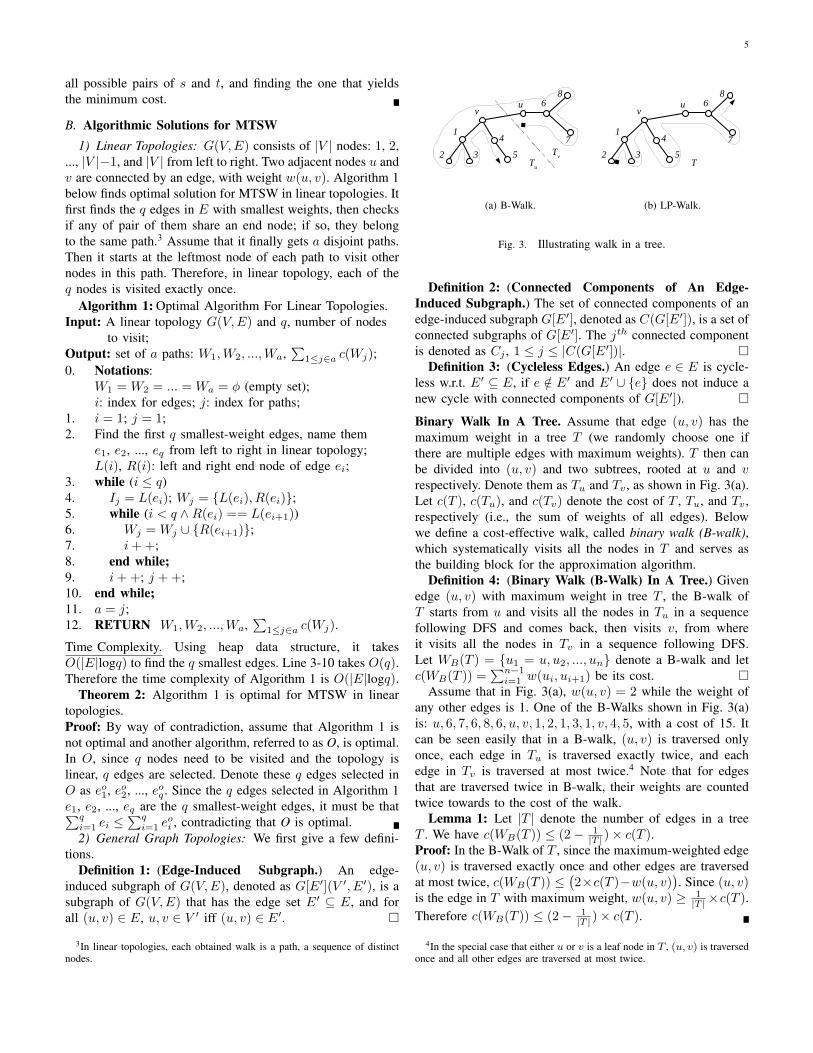
(a) B-Walk. (b) LP-Walk.

Fig. 3. Illustrating walk in a tree.

Definition 2: (Connected Components of An Edge-Induced Subgraph.) The set of connected components of anedge-induced subgraph G[E′], denoted as C(G[E′]), is a set ofconnected subgraphs of G[E′]. The jth connected componentis denoted as Cj , 1 ≤ j ≤ |C(G[E′])|. �

Definition 3: (Cycleless Edges.) An edge e ∈ E is cycle-less w.r.t. E′ ⊆ E, if e /∈ E′ and E′ ∪ {e} does not induce anew cycle with connected components of G[E′]). �

Binary Walk In A Tree. Assume that edge (u, v) has themaximum weight in a tree T (we randomly choose one ifthere are multiple edges with maximum weights). T then canbe divided into (u, v) and two subtrees, rooted at u and vrespectively. Denote them as Tu and Tv , as shown in Fig. 3(a).Let c(T ), c(Tu), and c(Tv) denote the cost of T , Tu, and Tv ,respectively (i.e., the sum of weights of all edges). Belowwe define a cost-effective walk, called binary walk (B-walk),which systematically visits all the nodes in T and serves asthe building block for the approximation algorithm.

Definition 4: (Binary Walk (B-Walk) In A Tree.) Givenedge (u, v) with maximum weight in tree T , the B-walk ofT starts from u and visits all the nodes in Tu in a sequencefollowing DFS and comes back, then visits v, from whereit visits all the nodes in Tv in a sequence following DFS.Let WB(T ) = {u1 = u, u2, ..., un} denote a B-walk and letc(WB(T )) =

∑n−1i=1 w(ui, ui+1) be its cost. �

Assume that in Fig. 3(a), w(u, v) = 2 while the weight ofany other edges is 1. One of the B-Walks shown in Fig. 3(a)is: u, 6, 7, 6, 8, 6, u, v, 1, 2, 1, 3, 1, v, 4, 5, with a cost of 15. Itcan be seen easily that in a B-walk, (u, v) is traversed onlyonce, each edge in Tu is traversed exactly twice, and eachedge in Tv is traversed at most twice.4 Note that for edgesthat are traversed twice in B-walk, their weights are countedtwice towards to the cost of the walk.

Lemma 1: Let |T | denote the number of edges in a treeT . We have c(WB(T )) ≤ (2− 1

|T | )× c(T ).Proof: In the B-Walk of T , since the maximum-weighted edge(u, v) is traversed exactly once and other edges are traversedat most twice, c(WB(T )) ≤

(2×c(T )−w(u, v)

). Since (u, v)

is the edge in T with maximum weight, w(u, v) ≥ 1|T |×c(T ).

Therefore c(WB(T )) ≤ (2− 1|T | )× c(T ).

4In the special case that either u or v is a leaf node in T , (u, v) is traversedonce and all other edges are traversed at most twice.

6

Approximation Algorithm For General Graph. Next wepresent an polynomial approximation algorithm (Algorithm 2),which yields a total cost of the walks that is at most (2− 1

q )times of the optimal cost. It works as follows. Line 1 sortsall the edges in E into nondecreasing order of their weights.Line 2 initializes the set Eq to the empty set and creates|V | trees, each containing one node. The while loop in lines3-9 checks each edge (in the nondecreasing order of theweight), if it is cycleless w.r.t. Eq . If yes, add it into Eq .This continues until q edges are added into Eq . It then obtainsall the connected components induced by these q edges. Sincethere is no cycles introduced during this process, each of thoseinduced connected components could only be a linear or a treetopology. If it is linear, it starts from one end and visits therest nodes in this linear topology exactly once; if it is a tree,it does a B-walk along the tree.

Algorithm 2: Approximation Algorithm For General Graphs.Input: A general graph G(V,E) and q, number of nodes

to visit;Output: set of a walks: W1,W2, ...,Wa, and

∑1≤j∈a c(Wj);

1. Let w(e1) ≤ w(e2) ≤ ... ≤ w(e|E|);2. Eq = φ (empty set), i = j = k = 1;3. while (k ≤ q)4. if (ei is a cycleless edge w.r.t. E′)5 Eq = Eq ∪ {ei};6. k ++;7. end if;8. i++;9. end while;10. Let |C(G[Eq])| = a;11. for (1 ≤ j ≤ a)12. if (Cj is linear) Starts from one end of Cj and

visits the rest nodes in Cj ;13. if (Cj is a tree) Do a B-walk along Cj ;14. Let the resulted walk (or path) be Wj ;15. end for;16. RETURN W1,W2, ...,Wa, and

∑1≤j∈a c(Wj).

Time Complexity and Discussions. Using disjoint-set datastructure, the running time of Algorithm 2 is O(|E|log|E|).Algorithm 2 works similarly as finding edges of minimumspanning trees in the well-known Kruskal’s algorithm [6],however, with two significant differences. First, instead offinding |V | − 1 edges that connect all the nodes in V ,Algorithm 2 only finds a set of q edges Eq , where q ≤ |V |−1.Therefore, instead of a single spanning tree that covers all thenodes in V resulted from Kruskal’s algorithm, Algorithm 2produces a forest, a graph with each connected component atree. Second, unlike Kruskal’s algorithm, which is an optimalalgorithm, traveling each of the trees following a B-walk givesrise of an approximation algorithm for an NP-hard problem(Theorem 3).

Definition 5: (Forest, q-Edge Forest, Cost of a Forest)A forest F of G is a subgraph of G with each connected

component a tree. A q-edge forest, denoted as Fq , is a forestwith q edges. The cost of a forest F , denoted as c(F ), is thesum of weights of all edges in F , c(F ) =

∑e∈F we. �

The cost of the forest induced by Eq in Algorithm 2 isc(Eq) =

∑e∈Eq

w(e) (here, we use Eq to also denote itsinduced forest when the context is clear). Next we prove thatc(Eq) is the minimum among the costs of all q-edge forests.

Lemma 2: c(Eq) ≤ c(F ),∀F ∈ Fq .Proof: Let E = {e1, e2, ..., e|E|}, with w(e1) ≤ w(e2) ≤ ... ≤w(e|E|). Let Eq = {eg1, e

g2, ..., e

gq}, with w(eg1) ≤ w(eg2) ≤

... ≤ w(egq) (this is the order in which they are selected inAlgorithm 2). By way of contradiction, assume that Eq is nota minimum-cost q-edge forest; instead Oq = {eo1, eo2, ..., eoq}is a minimum-cost q-edge forest, with w(eo1) ≤ w(eo2) ≤ ... ≤w(eoq).

Assume that egl ∈ Eq and eol ∈ Oq are the first pair ofedges that differ in Eq and Oq . That is, egl 6= eol and egi = eoi ,∀ 1 ≤ i ≤ l − 1. According to Algorithm 2, w(egl ) ≤ w(eol ).Now consider subgraph Oq ∪ {egl }. We have two cases.

Case 1: Oq ∪{egl } is a forest. Then c(Oq ∪{egl }−{eol }) ≤c(Oq), contradicting that Oq is a minimum cost q-edge forest.

Case 2: Oq ∪{egl } is not a forest, i.e., there is a cycle in it.egl must be in this cycle since Oq is a forest. Next we claimthat among all the edges in this cycle that is not egl , at least oneof them is not in {eg1, e

g2, ..., e

gl−1}; otherwise there will not be

any cycle. Denote this edge as e′. Let egl = en, 1 ≤ n ≤ |E|.We have two subcases.

Case 2.1: e′ ∈ {e1, e2, ..., en−1}. To be exact,e′ ∈ {e1, e2, ..., en−1} − {eg1, e

g2, ..., e

gl−1}. Thus w(e′) ≤

w(en−1) ≤ w(en) = w(egl ), contradicting that egl and eol arethe minimum edges that differ.

Case 2.2: e′ ∈ {en+1, en+2, ..., e|E|}. Thus w(e′) ≥w(en+1) ≥ w(en) = w(egl ). In this case, c(Oq ∪ {egl } −{e′}) ≤ c(Oq), contradicting that Oq is a minimum cost q-edge forest.

Reaching contradiction in all the cases, it concludes thatc(Eq) ≤ c(F ),∀F ∈ Fq .

Let O be an optimal algorithm of MTSW, which gives theminimum cost of O. Next we show that c(Eq) is a lowerbound of O.

Lemma 3: c(Eq) ≤ O.Proof: Without loss of generality, assume that the edgesselected in O induces o connected components, denoted asOj (1 ≤ j ≤ o). Assume that there are lj nodes in Oj , andsj ≥ 1 of them are starting nodes (therefore there are sj walksin Oj , visiting altogether lj − sj nodes). Let the cost of thesj walks in Oj be c(W o

j ),∑oj=1 c(W

oj ) = O.

Let c(Oj) denote the sum of weights of all edges in Oj ,c(Oj) =

∑e∈Oj

w(e). We have c(Oj) ≤ c(W oj ) since each

edge in Oj is traversed at least once in O. Next denote anytree of Oj as T oj , and denote the sum of all edges in T ojas c(T oj ). We have c(T oj ) ≤ c(Oj) ≤ c(W o

j ), resulting in∑oj=1 c(T

oj ) ≤

∑oj=1 c(W

oj ) = O.

Let q′ denote the total number of edges in the o connectedcomponents of O, q′ =

∑oj=1(lj − 1). The subgraph induced

by all T oj (1 ≤ j ≤ o) is therefore a q′-edge forest. Since

7

all together q nodes are visited,∑oj=1(lj − sj) = q. Since

sj ≥ 1, we have q ≤∑oj=1(lj − 1) = q′. Therefore, c(Eq) ≤

c(Eq′)Lemma 2≤

∑oj=1 c(T

oj ) ≤ O.

Theorem 3: Algorithm 2 is a (2− 1q )-approximation algo-

rithm for MTSW under general graph topologies, where q isnumber of distinct nodes to visit.Proof: Algorithm 2 finds a connected components, Cj (1 ≤j ≤ a), out of q selected edges Eq . Let qj and c(Cj) denote thenumber of edges in Cj and the sum of weights of edges in Cj ,respectively. We have q =

∑aj=1 qj and c(Eq) =

∑aj=1 c(Cj).

For any Cj , let c(Wj) denote sum of weights of all the edgestraversed in B-DFS walk Wj . Following Lemma 1, c(Wj) ≤(2− 1

qj)×c(Cj). Therefore, the total cost of the a walks found

in Algorithm 2 is:a∑j=1

c(Wj)Lemma 1≤

a∑j=1

((2− 1

qj)× c(Cj)

)

<

a∑j=1

((2− 1

q)× c(Cj)

)= (2− 1

q)× c(Eq)

Lemma 3≤ (2− 1

q)×O.

Smaller-Tree-First-Walk (STF-Walk). When a B-Walk tra-verses subtree Tu then Tv , each edge in Tu is traversed twicewhile each edge in Tv is traversed at most twice. Therefore, inorder not to traverse many edges twice, a simple improvementcould be to traverse, between Tu and Tv , the one with asmaller cost first. We refer to this as smaller-tree-first-walk(STF-Walk).

Heuristic Algorithm For General Graphs. Next we presenta heuristic algorithm to further improve the performance uponAlgorithm 2. It differs with Algorithm 2 only in line 13:Instead of a B-walk along each tree Cj (1 ≤ j ≤ a), it followsa longest-path-based walk defined as follows.

Definition 6: (Longest-Path Walk (LP-Walk) In A Tree.)Given a tree T , let P = {v1, v2, ..., vn} be the longest path inT . A LP-walk starts from v1, visiting all the nodes in T in asequence following DFS, and ends at vn, such that every edgein P is traversed exactly once. �

The novelty of the heuristic algorithm is based on theobservation that when more edges are traversed only once, thecost of a walk can be further reduced. One of the LP-walks inthe tree in Fig. 3(a) is now: 2, 1, 3, 1, v, 4, 5, 4, v, u, 6, 7, 6, 8, asshown in Fig 3(b). It has a cost of 14. Because the maximum-weight edge (u, v) is not necessarily on the longest path P ,we can not obtain performance guarantee for this heuristicalgorithm. However, we show via extensive simulations inSection V that it outperforms the approximation algorithm by20%− 30%, in terms of energy consumption, under differentnetwork parameters.

IV. Algorithmic Solutions for DRANext we transform the original sensor network graph

G(V,E) into an aggregation graph G′(V ′, E′), which is de-

fined below. We then show that solving DRA in G is equivalentto solving MTSW in G′.

Definition 7: (Aggregation Graph.) For a sensor networkgraph G(V,E), its aggregation graph G′(V ′, E′) is defined asfollows. V ′ is the set of p data nodes in V , i.e. V ′ = Vd.For any two data nodes u, v ∈ Vd in G, there exists an edge(u, v) ∈ E′ in G′ if and only if all the shortest paths betweenu and v in G do not contain other data nodes. For each edge(u, v) ∈ E′, its weight w(u, v) is the cost of the shortest pathbetween u and v in G. �

Theorem 4: DRA in G(V,E) is equivalent to MTSW inG′(V ′, E′).Proof: First, we argue that if all the shortest paths betweentwo data nodes X and Y in G do not contain any other datanodes, then in G′ they can be replaced by one single edge(X,Y ), whose weight is the cost of any of such shortest paths.As DRA concerns with visiting only data nodes followingshortest paths, all the storage nodes on the shortest pathsbetween X and Y in G do not appear in G′, as long as theenergy consumption of sending data from X to Y is accuratelycaptured. This is so since the weight of the edge (X,Y ) in G′

represents the energy consumption along these shortest paths.In Fig. 2, (B,E), (D,E), (D,G), (E, I), and (G, I) belongto this case. Otherwise, if at least one of the shortest pathsbetween data nodes X and Y contains other data nodes, edge(X,Y ) is not included in G′. In Fig. 2, (B, I) belongs to thiscase among others.

Second, if there exists multiple shortest paths between twodata nodes X and Y in G, some having at least another datanode as intermediate nodes and some not, we argue that theintermediate nodes in the ones without data nodes are notincluded in the G′. In order to visit as many data nodes(aggregators) as possible while using as least amount of energyas possible, it mandates that DRA takes a shortest path withdata nodes as intermediate nodes as part of the aggregationwalk. (B,D) and (E,G) in Fig. 2 belong to this case.

Above rules guarantee that essential information in G fordata aggregation, including data nodes and energy consump-tion sending data among them, are both accurately capturedin the aggregation G′. Therefore, solving MTSW in G′ isequivalent to solving DRA in G.

Fig. 4(a) shows the aggregation graph G′ of sensor networkgraph G in Fig. 2. Since 4 aggregators are needed (q = 4),using Algorithm 2, we find q-edge forest F of G′ (Fig. 4(b))and B-walk on F (Fig. 4(c)) sequentially.5 Finally, we obtainthe aggregation walk in G (Fig. 4(d)) by replacing each edge(u, v) in F with a shortest path between u and v in G (chooseone randomly if there are multiple).

We note the fundamental difference between aggregationgraph and metric completion of a graph. Metric completion ofG is a complete graph wherein the length of edge betweenevery pair of nodes in the graph equals to the length ofthe shortest path between them in G. The aggregation graphresembles the metric completion of graph in the definition of

5The LP-walk happens to be the same as B-walk in this example.

8

Fig. 4. (a) Aggregation graph G′ of sensor network graph G in Fig. 2, (b)q-edge forest F from G′, (c) B-walk (LP-walk) on F , and (d) Aggregationwalk in G. The numbers on edges are their weights.

0

5

10

15

20

25

30

35

40

45

50

26 28 30 32 34 36 38 40 42 44 46 48

Nu

mb

er

of

Ag

gre

ga

tors

q

Number of Data Nodes p

ρ=1ρ=0.7ρ=0.5ρ=0.3ρ=0.1

(a) Valid range of number of datanodes p, and number of aggregatorsq.

2 4 6 8

10 12 14 16 18 20 22 24

26 28 30 32 34 36 38 40 42 44 46 48

Ma

xim

um

Nu

mb

er

of

Initia

tors

p-q

Number of Data Nodes p

ρ=1ρ=0.7ρ=0.5ρ=0.3ρ=0.1

(b) Maximum number of initiatorsp− q.

Fig. 5. Feasible overall storage overflow with varying ρ (R = m).

the edge weight or length. However, aggregation graph of Gis not necessarily a complete graph, due to the intrinsic multi-hop nature of a wireless sensor network.

V. Performance EvaluationWe compare the performance of the approximation algo-

rithm (referred to as B-Walk) and the heuristic algorithm(referred to as LP-Walk). In our setup, 50 sensors are uni-formly distributed in a region of 1000m × 1000m square.Transmission range is 250m; two sensor nodes can com-municate directly if their distance is within the transmissionrange. Unless otherwise mentioned, the storage capacity ofeach storage node m is 512KB, the size of overflow data ateach data node R is 512KB. We define correlation coefficientas ρ = 1 − r/R, where r is the size of overflow data afteraggregation at each aggregator. The more correlation amongdata, the larger ρ is: ρ = 0 means no correlation at all, whileρ = 1 means perfect correlation (i.e., data at aggregatorsare duplicate copies of data at data nodes therefore can becompletely removed). However, ρ = 0 is not considered insimulations since data correlation exists.

Feasible Overall Storage Overflow. Given |V |,m,R, r,Equation 1 gives the valid range of number of data nodesp for a feasible overall storage overflow. Given each validp, Equation 2 finds its corresponding number of aggregatorsq that should be visited, therefore p − q are the maximumnumber of allowable data nodes that can serve as initators. To

investigate the feasible overall storage overflow, we study asensor network with 50 nodes and set R = m.

Fig. 5(a) shows for different ρ, the valid range of p and thecorresponding value of q for each value of p. When ρ = 0.1,the valid range of p is a single value of 26, with correspondingvalue of q 20. When increasing ρ, the valid range of p expands,from 26-29 in ρ = 0.3, to 26-33 in ρ = 0.5, to 26-37 inρ = 0.7, to 26-49 in ρ = 1. This is because more datacorrelation leads to more data aggregation, thus more datanodes are allowed while satisfying feasible overflow condition.It also shows that for each ρ, q increases when increasing p.This is because more data nodes means more overflow dataand less available storage, therefore more aggregators need tobe visited to achieve enough data size reduction.

Consequently, less number of data nodes can serve asinitiators, i.e., p − q decreases with the increase of p, asshown in Fig. 5(b). It also shows that for the same p, p − qincreases with the increase of ρ. This is implied by Equation 2,which can be written as: q = dp×(1+m/R)−|V |×m/R

ρ e. Whenp is fixed, more data correlation means that less number ofaggregators are needed in order to reduce data size, thereforemore data nodes can serve as initiators. Finally, Fig. 5(b)indicates that there are two cases in which only one initiatoris allowed: ρ = 0.5 and p = 33, and ρ = 1 and p = 49, whilemultiple initiators are allowed for other cases.

Comparing SFT-Walk with B-Walk. We first compare SFT-Walk with B-Walk, where SFT-Walk traverses the smallersubtree first while B-Walk randomly chooses one of the twosubtrees to traverse first. We choose ρ = 0.5 and vary p from26 to 33. Fig. 6(a) shows that when p is small, both yieldthe same aggregation costs because the resulted trees are alllinear topologies. However, when p gets larger, the aggregationcost of SFT-Walk is less than that of B-Walk. This is becauseSFT-Walk traverses the edges of the smaller subtree twicewhile B-Walk could possibly traverse the edges of the biggersubtree twice. Fig. 6(b) shows the performance improvementof SFT-Walk over B-Walk, which is the difference of theircosts divided by the cost of B-Walk. In general, SFT-Walkimproves B-Walk by 5− 10%. We therefore adopt SFT-Walkfor B-Walk for the rest of the simulations, and still refer it toas B-Walk.

Comparing B-Walk with LP-Walk Visually. Next we visu-ally compare the performances of B-Walk and LP-Walk in anetwork of 50 nodes, for both cases of single initiator andmultiple initiators.Single Initiator. When ρ = 0.5 and p = 33, q = 32 andp− q = 1. That is, there are 32 aggregators and one initiator.Fig. 7(a) and (b) show such a sensor network graph and itsaggregation graph, respectively. Fig. 7(c) and (d) show theaggregation walks from B-Walk and LP-Walk, respectively. B-Walk visits 32 edges twice, resulting in a total cost of 381.2J ;while LP-Walk only visits 12 edges twice, with a total cost of290.6J , a 23.8% of improvement upon B-Walk.Multiple Initiators. When ρ = 0.5 and p = 32, q = 28 andp − q = 4. That is, there are 29 aggregators and at most 4

9

(a) Sensor network graph. (b) Aggregation graph. (c) B-Walk (cost=381.2J). (d) LP-Walk (cost=290.6J).

Fig. 7. Visually comparing B-Walk and LP-Walk with one initiator. � and J– indicate initiators and aggregators that are last visited.

(a) Sensor network graph. (b) Aggregation graph. (c) B-Walk (cost=255.9J). (d) LP-Walk (cost=203.0J).

Fig. 8. Visually comparing B-Walk and LP-Walk when 4 initiators are allowed.

0

50

100

150

200

250

300

350

400

450

500

26 27 28 29 30 31 32 33

To

tal A

gg

reg

atio

n C

ost

(J)

Number of Data Nodes p

STF-WalkB-Walk

(a) Total Aggregation Cost.

0 %

5 %

10 %

15 %

20 %

26 27 28 29 30 31 32 33

Pe

rfo

rma

nce

Im

pro

ve

me

nt

of

ST

F-W

alk

up

on

B-W

alk

Number of Data Nodes p

(b) Performance Improvement ofSFT-Walk Upon B-Walk.

Fig. 6. Comparing STF-Walk and LP-Walk.

initiators. Fig. 8 shows that B-walk aggregation traverses 19edges twice, resulting in a total cost of 255.9J , while LP-Walk aggregation traverses 9 edges twice, with a total costof 203.0J , a 20.7% of improvement. Among the four treesin q-edge forest, B-Walk and LP-Walk find exactly the sameaggregation walks in two smaller ones. This shows that whenincreasing number of initiators, the performance differencebetween B-Walk and LP-Walk gets smaller. This is becausewith more initiators, the resulted q-edge forest consists of more

trees with smaller sizes, each with a “short” longest path. Bytraversing the edges on such short longest paths once, LP-Walk does not save as much at it can compared to traversinga big tree with much longer longest path. Finally, comparedto single initiator case, both B-Walk and LP-Walk incur lessenergy cost, because more initiators can now be utilized tofind more cost-effective aggregation walks.

Comparing B-Walk and LP-Walk by Varying p and ρ. Nextwe study the aggregation costs of B-Walk and LP-Walk, andthe performance difference between them, by considering thewhole ranges of p and ρ, that is, ρ = 0.1, 0.3, 0.5, 0.7, 1.0 andp ∈ [26, 49]. Fig. 9(a) shows that for each ρ, with the increaseof p, the total aggregation costs of both B-Walk and LP-Walkincrease. However, LP-Walk constantly perform better than B-Walk. It also shows that for the same p, with the increase of ρ,the aggregation costs for both B-Walk and LP-Walk decreases.This is because more correlation means that less number ofaggregators need to be visited, reducing aggregation costs.

Fig. 9(b) calculates the performance improvement of LP-Walk upon B-Walk, which is defined as (total aggregationcost of B-Walk - total aggregation cost of LP-Walk)/ totalaggregation cost of B-Walk. It shows that for each ρ, ineach of its own valid range of p, the smaller the ρ, thelarger of the performance improvement when p is fixed. For

10

example, when p = 26 (the only valid value for ρ = 0.1), theperformance improvement for ρ = 0.1 is 14% while zero forρ = 0.3, 0.5, 0.7, 1.0. When ρ = 0.5, in its valid p range (26-33), it almost always has a larger performance improvementcompared to ρ = 0.5, 0.7, 1. When less data correlation exists,more aggregators need to be visited, therefore the resultedq-edge forest gets larger as well as its constituent trees. Bytraversing the longest paths of larger trees once, LP-Walk cansave more aggregation cost compared to traversing a smallertree. This explains why LP-Walk has a larger performanceimprovement upon B-Walk when ρ gets smaller.

0

100

200

300

400

500

26 28 30 32 34 36 38 40 42 44 46 48

To

tal A

gg

reg

atio

n C

ost

(J)

Number of Data Nodes p

ρ=1, B-Walkρ=1, LP-Walk

ρ=0.7, B-Walkρ=0.7, LP-Walk

ρ=0.5, B-Walkρ=0.5, LP-Walk

ρ=0.3, B-Walkρ=0.3, LP-Walk

ρ=0.1, B-Walkρ=0.1, LP-Walk

(a) Total Aggregation Cost.

0 %

5 %

10 %

15 %

20 %

25 %

26 28 30 32 34 36 38 40 42 44 46 48

Pe

rfo

rma

nce

Im

pro

ve

me

nt

of

LP

-Wa

lk u

po

n B

-Wa

lk

Number of Data Nodes p

ρ=1ρ=0.7ρ=0.5ρ=0.3ρ=0.1

(b) Performance Improvement ofLP-Walk Upon B-Walk.

Fig. 9. Comparing B-Walk and LP-Walk by Varying p and ρ.

Comparing B-Walk and LP-Walk by Varying R/m. Finally,we compare the performances of B-Walk and LP-Walk basedon different ratios of R/m. When increasing R/m, the overallstorage overflow situations deteriorate since more overflowdata needs to be accommodated. We set ρ = 0.5 and varyR/m from 1 to 5. The common range of p for differentratios of R/m is [26, 30], therefore we pick 26 and 30for p. Fig. 10(a) shows the total aggregation costs for bothB-Walk and LP-Walk, when p = 26 and 30. Fig. 10(b)calculates the performance improvement of LP-Walk upon B-Walk, which is shown to increase generally when increasingR/m. This indicates that LP-Walk performs even better inmore challenging overall storage overflow scenarios.

0

50

100

150

200

250

300

350

400

1 2 3 4 5

To

tal A

gg

reg

atio

n C

ost

(J)

R/m

p=26,B-Walkp=26,LP-Walk

p=30,B-Walkp=30,LP-Walk

(a) Total Aggregation Cost.

0 %

5 %

10 %

15 %

20 %

25 %

1 1.5 2 2.5 3 3.5 4 4.5 5

Pe

rfo

rma

nce

Im

pro

ve

me

nt

of

LP

-Wa

lk u

po

n B

-Wa

lk

R/m

p=26p=30

(b) Performance Improvement ofLP-Walk Upon B-Walk.

Fig. 10. Comparing B-Walk and LP-Walk by Varying R/m.

VI. Related WorkBelow, we categorize and review the prior work in data

resilience in sensor networks, data aggregation in sensornetworks, and related graph-theoretic research.

A. Data Resilience in Sensor Networks.

Many data resilience techniques have been proposed to over-come against different causes of data loss in sensor networks.Ghose et al. [11] are among the first to propose Resilient Data-Centric Storage (R-DCS) to achieve resilience by replicatingdata at strategic locations in the sensor network. Ganesan [10]consider constructing partially disjoint multipaths to enableenergy efficient recovery from failure of the shortest pathbetween source and sink. Recently, network coding techniquesare used to recover data from failure-prone sensor networks.Albano et al. [1] propose in-network erasure coding to improvedata resilience to node failures. Kamra et al. [18] propose toreplicating data compactly at neighboring nodes using growthcodes that increase in efficiency as data accumulates at thesink. However, all these data resilience measures adopt thetraditional sensor network model wherein base stations arealways available near or inside the networks. Therefore, allthe data resilience measures are designed towards transmittingdata reliably to the base station.

Recently, some data resilience research has focused onhow to preserve data in disconnection-tolerant storage sensornetwork in the absence of base station. We are aware of twolines of work in this direction. The first line is a sequenceof system research [26, 27, 38, 44]. Since no base station isavailable, they design cooperative distributed storage systemsspecifically for disconnected operations of sensor networks, toimprove the utilization of the networks data storage capacity.The other line of research instead takes an algorithmic ap-proach by focusing on the hardness of the data preservationproblems and the optimality of their solutions [14, 35, 43].Tang et al. [35] address the energy-efficient data redistributionproblem in data-intensive sensor networks. Hou et al. [14]study how to maximize the minimum remaining energy of thenodes that finally store the data, in order to store the datafor long period of time. Xue et al. [43] consider that sensorydata from different source nodes have different importance,and study how to preserve data with highest importance.However, all above work assume that there is enough storagespace available from the network to hold all the overflow dataand none of above work address the overall storage overflowproblem.

B. Data Aggregation in Sensor Networks.

There is vast amount of literature of data aggregation insensor networks. Here we only review the most recent andmost related works. Tree-based routing structures are oftenproposed to either maximize the network lifetime (the timeuntil the first node depletes its energy) [25, 41], or minimizethe total energy consumption or communication cost [19, 22],or reduce the delay of data gathering [42]. In DRA, since thebase station is not available and data must be stored inside

11

the network, tree-bases routing structure is no longer suitable.Instead, our data aggregation process follows a routing schemethat resembles traveling salesman problem [21]. Some worksare based on non-tree routing structures and propose usingmobile base stations to collect aggregated data in order tomaximize the network lifetime [34, 36]. In contrast, we insteadaddress a very different scenario for sensor networks: beforethe mobile base stations or data mules become available,some sensor nodes already deplete their storage, therefore theirnewly generated data must be offloaded to other sensor nodeswith available storage. The challenge lies in the fact that thetotal generated data in the network overflows the total availablestorage in the network. To the best of our knowledge, theoverall storage overflow problem has not been addressed byany of the existing data aggregation research.

C. Overview of Related Theoretical Problems.

Below we give a brief overview of the well-known travelingsalesman problem (TSP) [21] and the related vehicle routingproblem (VRP) [37], which are both NP-hard, and identify thedifferences between these problems and the MTSW.

TSP asks the following question: Given a list of citiesand the distances between each pair of cities, what is theshortest possible route that visits each city exactly once andreturns to the origin city? A recent book by Gutin et al.[12] provide a compendium of results on the problem. Themultiple traveling salesman problem (mTSP) [3] extends TSPto multiple salesman and determines a tour for each salesmansuch that the total tour cost is minimized and that each city isvisited exactly once by one salesman. VRP refers to a wholeclass of problems involving the visiting of “customers” by“vehicles”, wherein each customer has a positive demand andeach vehicle has a limited capacity serving the demands. Thegoal of VRP is to find a route for each vehicle in order tosupply all the customers and minimize the total cost of theroutes. VRP is a generalization of the mTSP by consideringdemands from “customers” and “capacity” of the vehicles.Toth and Vigo [37] given an up-to-date survey of the variantsand solution techniques for VRP.

The differences between mTSP/VRP and MTSW is asfollows. Unlike mTSP, not only does MTSW need to figureout the order in which to visit cities, but it must answer someother fundamental questions: from which cities are salesmendispatched and which cities does each salesman visit? In VRP,the set of vehicle locations (the depots) and the set of customerlocations are usually disjoint. There is no such distinction fornodes in MTSW – each node can either dispatch a salesman(i.e. a vehicle) or be visited (i.e. as a customer). In VRP, a fixedset of customers (or cities) must be visited while in MSTW, itonly requires all together q cities are visited, not necessarily aspecific subset of cities. In VRP, each vehicle route starts andends at the same or different depots while MSTW does nothave such constraint.

The traveling salesman path problem (TSPP) [20] is definedas follows. Given an undirected graph G = (V,E), a costfunction on the edges, and two nodes s, t ∈ V , the TSPP is to

find a Hamiltonian path from s to t visiting all cities exactlyonce (the case s = t is equivalent to the TSP). Instead ofa Hamiltonian path from s to t, the traveling salesman walk(TSW) problem [20] asks for the minimum cost s−t travelingsalesman walk, wherein the traveling salesman walk visits allvertices at least once. The MTSW we study is essentially amultiple traveling salesman walk problem, wherein up to somenumber of salesman can be dispatched from some cities, suchthat total q cities are visited with minimum amount of cost.

VII. Conclusion and Future WorkIn this paper we solve overall storage overall problem in

sensor networks by designing close-to-optimal data aggrega-tion algorithms. Even though DRA is uniquely derived fromsensor networks, it is a theoretically fundamental problem aswell as a practical problem potentially with other applications.Its theoretical rigor lies in the underlying multiple travelingsalesman walk problem, a new variation of the classic travelingsalesman problem that has not been studied. Because of thistheoretical root, the techniques proposed in this paper could beapplicable not only in sensor networks, but in any applicationsin which data correlation and resource constraints coexist, suchas scientific application, data centers, and big data analytics.

As future work, we will augment the proposed techniquesto tackle situations with some nodes depleting their batterypower, and design distributed algorithms for DRA. Currentlythe DRP is a static problem, in which the overflow data isgenerated at the beginning and only once. We will address areal-time problem where data is generated and transmitted dy-namically and periodically, and investigate how the dynamicsaffect the problem and its solutions.

After being aggregated to the size accommodable by theavailable storage capacity, the overflow data need to be of-floaded to storage nodes to be stored. Therefore the DRA isonly the first stage of a more broad overall storage overflowin sensor networks. The second stage of offloading aggregateddata from data nodes/aggregators to storage nodes has beenstudied extensively by existing research [14, 35, 43]. An inter-esting question to ask is: Should the data resilience measurebe treated as two separate stages of data aggregation and thendata offloading, or should it be treated in a holistic approach?In another word, is an optimal data aggregation plus an optimaldata offloading optimal for the whole problem? The answeris no. For example, in Fig. 2, there are two optimal dataaggregation solutions: B is the initiator and its aggregationwalk is: B, E, D, G, H , I; or I is the initiator and itsaggregation walk is: I , H , G, D, E, B. However, the formerachieves optimal for the whole problem while the latter not.As an ongoing and future work, we would like to integratethese two stages together to explore a more energy-efficientsolution for the overall storage overflow problem.

REFERENCES

[1] Michele Albano and Jie Gao. Resilient data-centric storage in wirelessad-hoc sensor networks. In Proc. of the International Workshop on Algo-rithms for Sensor Systems, Wireless Ad Hoc Networks and AutonomousMobile Entities (ALGOSENSOR’10), pages 105–117, 2010.

12

[2] Salah A. Aly, Zhenning Kong, and Emina Soljanin. Fountain codesbased distributed storage algorithms for large-scale wireless sensornetworks. In Proc. of IPSN, 2008.

[3] Tolga Bektas. The multiple traveling salesman problem: an overviewof formulations and solution procedures. Elsevier Omega, 34:209–219,2006.

[4] Costas Busch, Malik Magdon-Ismail, Fikret Sivrikaya, and Bulent Yener.Contention-free mac protocols for wireless sensor networks. In Proc. ofDISC, pages 245–259, 2004.

[5] Harsha Chenji and Radu Stoleru. Mobile sensor network localizationin harsh environments. In Proceedings of the 6th IEEE internationalconference on Distributed Computing in Sensor Systems (DCOSS’10),pages 244–257, 2010.

[6] Thomas Corman, Charles Leiserson, Ronald Rivest, and Clifford Stein.Introduction to Algorithms. MIT Press, 2009.

[7] R. Cristescu, B. Beferull-Lozano, M. Vetterli, and R. Wattenhofer.Network correlated data gathering with explicit communication: Np-completeness and algorithms. IEEE/ACM Transactions on Networking,14:41–54, 2006.

[8] Rzvan Cristescu, Baltasar Beferull-lozano, Martin Vetterli, and RogerWattenhofer. On network correlated data gathering. In Proceedings ofIEEE Infocom, pages 2571–2582, 2004.

[9] John Heidemann Fred Stann. Rmst: Reliable data transport in sensornetworks. In Proc. of 1st IEEE International Workshop on Sensor NetProtocols and Applications (SNPA), pages 1–9, 2003.

[10] Deepak Ganesan, Ramesh Govindan, Scott Shenker, and Deborah Estrin.Highly-resilient, energy-efficient multipath routing in wireless sensornetworks. SIGMOBILE Mob. Comput. Commun. Rev., 5(4):11–25,October 2001.

[11] Abhishek Ghose, Jens Grossklags, and John Chuang. Resilient data-centric storage in wireless ad-hoc sensor networks. In Proceedings the4th International Conference on Mobile Data Management (MDM03,pages 45–62, 2003.

[12] G. Gutin and A. Punnen, editors. The Traveling Salesman Problem andits Variation. Kluwer Academic Publishers, 2002.

[13] W. Heinzelman, A. Chandrakasan, and H. Balakrishnan. Energy-efficientcommunication protocol for wireless microsensor networks. In Proc. ofHICSS 2000.

[14] Xiang Hou, Zane Sumpter, Lucas Burson, Xinyu Xue, and Bin Tang.Maximizing data preservation in intermittently connected sensor net-works. In Proc. of IEEE MASS 2012, pages 448–452.

[15] S. Jain, R. Shah, W. Brunette, G. Borriello, and S. Roy. Exploitingmobility for energy efficient data collection in wireless sensor networks.MONET, 11(3):327–339, 2006.

[16] Jaein Jeong, Xiaofan Jiang, and D. Culler. Design and analysis of micro-solar power systems for wireless sensor networks. In Proceedings of 5thInternational Conference on Networked Sensing Systems (INSS 2008),pages 181 – 188, 2008.

[17] Milica Stojanovic John Heidemann and Michele Zorzi. Underwatersensor networks: applications, advances and challenges. Phil. Trans.R. Soc. A, 370:158 – 175, 2012.

[18] Abhinav Kamra, Jon Feldman, Vishal Misra, and Dan Rubenstein.Growth codes: Maximizing sensor network data persistence. In Pro-ceedings of ACM Sigcomm, 2006.

[19] Tung-Wei Kuo and Ming-Jer Tsai. On the construction of data aggre-gation tree with minimum energy cost in wireless sensor networks: Np-completeness and approximation algorithms. In Proceedings of IEEEINFOCOM, pages 2591 – 2595, 2012.

[20] Fumei Lam and Alantha Newman. Traveling salesman path problems.Mathematical Programming, 113:39 – 59, 2008.

[21] E. Lawler, J.K. Lenstra, A.H.G. Rinnooy Kan, and D. SHmoys (Eds.).The Traveling Salesman Problem: A Guided Tour of CombinationalOptimization. John Wiley and Sons, 1985.

[22] Jian Li, Amol Deshpande, and Samir Khuller. On computing compres-sion trees for data collection in wireless sensor networks. In Proceedingsof INFOCOM, pages 2115–2123, 2010.

[23] Ke Li, Chien-Chung Shen, and Guaning Chen. Energy-constrained bi-objective data muling in underwater wireless sensor networks. In Proc.of the 7th IEEE International Conference on Mobile Ad-hoc and SensorSystems (MASS 2010), pages 332–341, 2010.

[24] Yunfeng Lin, Ben Liang, and Baochun Li. Data persistence in large-scale sensor networks with decentralized fountain codes. In Proc. ofINFOCOM, 2007.

[25] D. Luo, X. Zhu, X. Wu, and G. Chen. Maximizing lifetime forthe shortest path aggregation tree in wireless sensor networks. InProceedings of IEEE INFOCOM, pages 1566 – 1574, 2011.

[26] L. Luo, Q. Cao, C. Huang, L. Wang, T. Abdelzaher, and J. Stankovic.Design, implementation, and evaluation of enviromic: A storage-centricaudio sensor network. ACM Transactions on Sensor Networks, 5(3):1–35, 2009.

[27] L. Luo, C. Huang, T. Abdelzaher, and J. Stankovic. Envirostore:A cooperative storage system for disconnected operation in sensornetworks. In Proc. of INFOCOM 2007.

[28] Ming Ma and Yuanyuan Yang. Data gathering in wireless sensornetworks with mobile collectors. In Proc. of the IEEE InternationalSymposium on Parallel and Distributed Processing (IPDPS 2008), pages1–9, 2008.

[29] K. Martinez, R. Ong, and J.K. Hart. Glacsweb: a sensor network forhostile environments. In Proc. of SECON 2004.

[30] Ioannis Mathioudakis, Neil M. White, and Nick R. Harris. Wirelesssensor networks: Applications utilizing satellite links. In Proc. of theIEEE 18th International Symposium on Personal, Indoor and MobileRadio Communications (PIMRC 2007), pages 1–5, 2007.

[31] Univ. of Pittsburgh Pittsburgh PA USA ; Gadola G. Mosse, D. ; Comput.Sci. Dept. Controlling wind harvesting with wireless sensor networks.In Proceedings of International Green Computing Conference (IGCC),pages 1 – 6, 2012.

[32] Luca Mottola. Programming storage-centric sensor networks withsquirrel. In Proceedings of the ACM/IEEE IPSN, pages 1–12, 2010.

[33] Sundeep Pattem, Bhaskar Krishnamachari, and Ramesh Govindan. Theimpact of spatial correlation on routing with compression in wirelesssensor networks. ACM Trans. Sen. Netw., 4(4):1–33, September 2008.

[34] Yi Shi and Y.T. Hou. Theoretical results on base station movementproblem for sensor network. In Proceedings of IEEE INFOCOM, 2008.

[35] Bin Tang, Neeraj Jaggi, Haijie Wu, and Rohini Kurkal. Energy efficientdata redistribution in sensor networks. ACM Transactions on SensorNetworks, 9(2), May 2013.

[36] S. Tang, J. Yuan, X. Li, Y. Liu, G. Chen, M. Gu, J. Zhao, and G. Dai.Dawn: Energy efficient data aggregation in wsn with mobile sinks.In Proceedings of 18th International Workshop on Quality of Service(IWQoS), 2010.

[37] Paolo Toth and Daniele Vigo, editors. The Vehicle Routing Problem.Society for Industrial and Applied Mathematics, 2001.

[38] Lili Wang, Yong Yang, Dong Kun Noh, Hieu Le, Tarek Abdelzaher,Michael Ward, and Jie Liu. Adaptsens: An adaptive data collection andstorage service for solar-powered sensor networks. In Proc. of the 30thIEEE Real-Time Systems Symposium (RTSS 2009).

[39] B. Weiss, , H.L. Truong, W. Schott, A. Munari, C. Lombriser, U. Hun-keler, and P. Chevillat. A power-efficient wireless sensor network forcontinuously monitoring seismic vibrations. In Proceedings of IEEESECON, pages 37 – 45, 2011.

[40] Geoff Werner-Allen, Konrad Lorincz, Jeff Johnson, Jonathan Lees, andMatt Welsh. Fidelity and yield in a volcano monitoring sensor network.In Proc. of OSDI 2006.

[41] Y. Wu, S. Fahmy, and N. B. Shroff. On the construction of a maximum-lifetime data gathering tree in sensor networks: Np-completeness andapproximation algorithms. In Proceedings of IEEE INFOCOM, pages1566 – 1574, 2008.

[42] X. Xu, M. Li, X. Mao, S. Tang, and S. Wang. A delay-efficientalgorithm for data aggregation in multihop wireless sensor networks.IEEE Transactions on Parallel and Distributed Systems, 22:163 – 175,2011.

[43] Xinyu Xue, Xiang Hou, Bin Tang, and Rajiv Bagai. Data preservation inintermittently connected sensor networks with data priorities. In Proc.of IEEE SECON 2013, pages 65–73.

[44] Yong Yang, Lili Wang, Dong Kun Noh, Hieu Khac Le, and Tarek F.Abdelzaher. Solarstore: enhancing data reliability in solar-poweredstorage-centric sensor networks. In Proceedings of the 7th internationalconference on Mobile systems, applications, and services (MobiSys),year = 2009,.

[45] M. Z. Zamalloa and B. Krishnamachari. An analysis of unreliability andasymmetry in low-power wireless links. ACM Transactions on SensorNetworks, 3(2):1277–1280, 2007.