DATA MINING - CLUSTERING. Clustering 4 Clustering - unsupervised classification 4 Clustering - the...

DATA MINING - CLUSTERING

Clustering

Clustering - unsupervised classification Clustering - the process of grouping

physical or abstract objects into classes of similar objects

Clustering - help in construct meaningful partitioning of a large set of objects

Data clustering in statistics, machine learning, spatial database and data mining

CLARANS Algorithm

CLARANS - Clustering Large Applications Based on Randomized Search - presented by Ng and Han

CLARANS - based on randomized search and 2 statistics algorithm: PAM and CLARA

Method of algorithm - search of local optimum

Example of algorithm usage

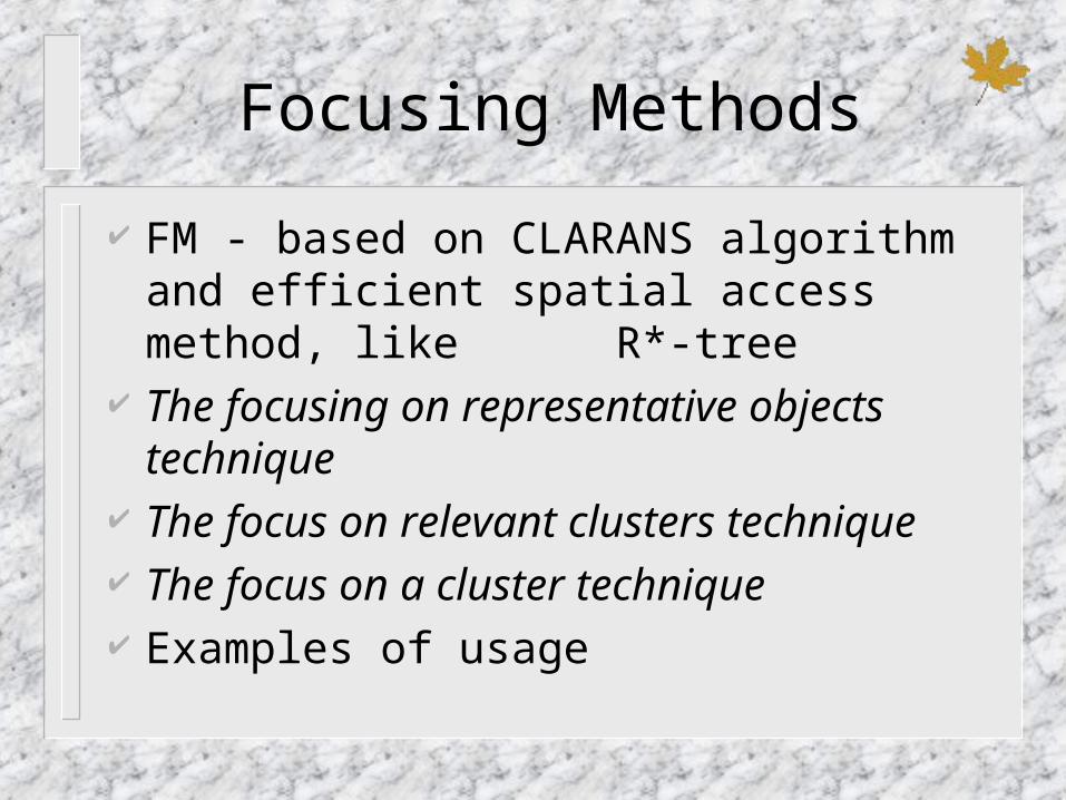
Focusing Methods

FM - based on CLARANS algorithm and efficient spatial access method, like R*-tree

The focusing on representative objects technique

The focus on relevant clusters technique The focus on a cluster technique Examples of usage

Pattern-Based Similarity Search

Searching for similar patterns in a temporal or spatial-temporal database

Two types of queries encountered in data mining operations:– object - relative similarity query– all -pair similarity query

Various approaches:– similarity measures chosen– type of comparison chosen– subsequence parameters chosen

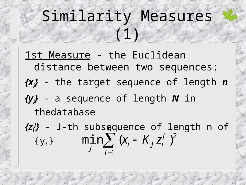
Similarity Measures (1)

1st Measure - the Euclidean distance between two sequences:

{xi} - the target sequence of length n

{yi} - a sequence of length N in thedatabase

{ziJ} - J-th subsequence of length n of {yi}

2

1

)(min

n

i

JiJi

JzKx

Similarity Measures (2)

3th Measure - the correlation

(Discrete Fourier Transforms)

between two sequences:

2nd Measure - the linear

correlation between two

sequences:

N

jj

n

jj

n

jjij

i

yx

yx

c

1

2

1

2

1

N

jj

n

jj

jji

YX

YXFc

1

2

1

2

*1 }{

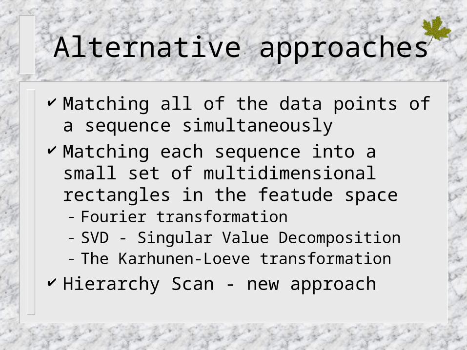
Alternative approaches

Matching all of the data points of a sequence simultaneously

Matching each sequence into a small set of multidimensional rectangles in the featude space – Fourier transformation– SVD - Singular Value Decomposition– The Karhunen-Loeve transformation

Hierarchy Scan - new approach

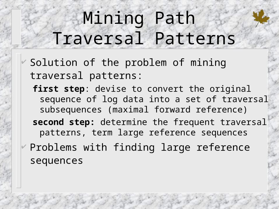
Mining Path Traversal Patterns

Solution of the problem of mining traversal patterns:first step: devise to convert the original sequence

of log data into a set of traversal subsequences (maximal forward reference)

second step: determine the frequent traversal patterns, term large reference sequences

Problems with finding large reference sequences

Mining Path Traversal Patterns - Example

Traversal path for a user:

{A,B,C,D,C,B,E,G,H,G,W,A,O,U,O,V}

V

C

B

GD

WH

O

E

A

U

2

34

5

7

6

98

15

11

1314

12

10

1

The set of maximal forward references for this user:{ ABCD, ABEGH, ABEGW, AOU, AOV }

Clustering Features and CF-trees

Clustering Features -

triplet summarizing

information about

subclusters of points:

N

ii

N

ii XSSXLS

SSLSNCF

1

2

1

,

),,(

CF-tree - a balanced

tree with 2 parameters: branching factor B -

max number of children threshold T - max

diameter of subclusters stored at the leaf nodes

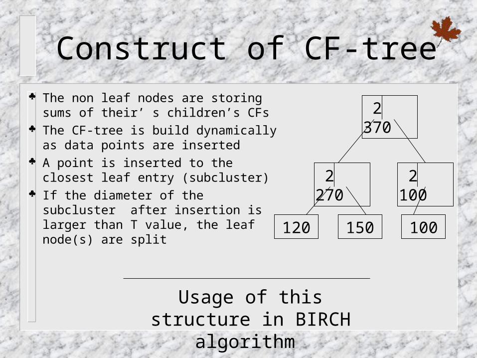
Construct of CF-tree

Usage of this structure in BIRCH algorithm

2 370

150120

2 270 2 100

100

The non leaf nodes are storing sums of their’ s children’s CFs

The CF-tree is build dynamically as data points are inserted

A point is inserted to the closest leaf entry (subcluster)

If the diameter of the subcluster after insertion is larger than T value, the leaf node(s) are split

BIRCH Algorithm

- Balanced

- Interactive

- Reducing and

- Clustering using

- Hierarchies

BIRCH Algorithm (1)

PHASE 1

Scan all data and built an initial in memory CF tree using the given amount of memory and recycling space on disk

Phase 1: Load into memory

Phase 2: Condense

Phase 3: Global Clustering

Phase 4: Cluster Refining

Data

BIRCH Algorithm (2)

PHASE 2 (optional)

Scan the leaf entries in the initial CF tree to rebuild a smaller CF tree, while removing more outliers and grouping crowded clusters into largest one



Data


Phase 2: Condense

BIRCH Algorithm (3)

PHASE 3

Adapt an existing clustering algorithm for a set of data points to work with a set of subclusters, each described by its CF vector.



Data


Phase 2: Condense

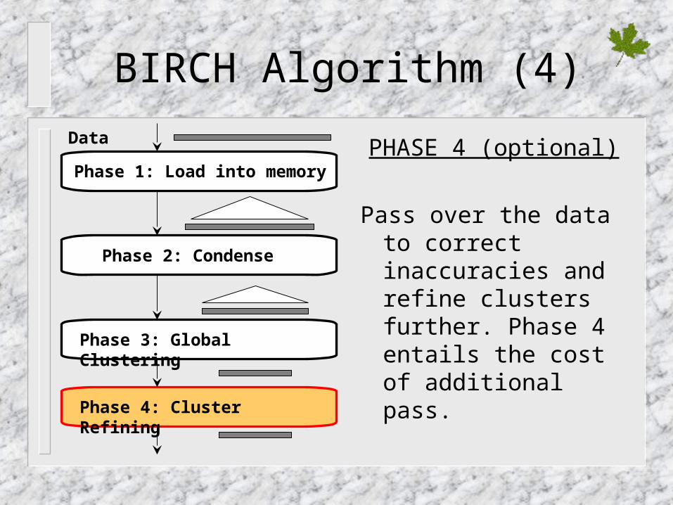
BIRCH Algorithm (4)

PHASE 4 (optional)

Pass over the data to correct inaccuracies and refine clusters further. Phase 4 entails the cost of additional pass.



Data


Phase 2: Condense

CURE Algorithm

- Clustering

- Using

- Representatives

CURE Algorithm (1)

Draw random sample Partition sample Partially cluster partitions

Label data in disk Cluster partial clusters Eliminate outliers

Data

CURE begins by drawing random sample from the database.

CURE Algorithm (2)



Data

In order to further speed up clustering, CURE first partition the random sample into p partitions, each of size n/p.

CURE Algorithm (3)



Data

Partially cluster each partition until the final number of clusters in each partition reduce to n/pq for some constant q > 1.

CURE Algorithm (4)



Data

Outliers do not belong to any of the clusters.

In CURE outliers are eliminated at multiply steps.

CURE Algorithm (5)



Data

Cluster in a final pass to generate the final k clusters.

CURE Algorithm (6)



Data

Each data point is assigned to the cluster containing the representative point closest to it.

CURE - cluster procedure

procedure cluster(S,k)begin T := build_kd_tree(S) Q := buid_heap(S) while size(Q) > k do { u := extract_min(Q) v := u.closet delete(Q,v) w := merge(u,v) delete_rep(T,u) delete_rep(T,u) insert_rep(T,w) w.closet := x /*x is an arbitrary cluster in Q */

for each xQ do { if dist(w,x) < dist(w,w.closet) w.closet := x if x.closet is either u or v { if dist(x,x.closet)< dist(x,w) a.closet := closet_cluster(T,x,dist(x,w)) else x.closet :=w relocate(Q,x) }else if dist(x,x.closet)>dist(x,w){ x.closet := w relocate(Q,x) } }insert (Q,w) }end

CURE - merge procedure

procedure merge(u,v)begin w := uUv w.mean := |u|u.mean+|v|v.mean/|u|+|v| tmpSet := for i := 1 to c do { maxDist := 0 foreach point p in cluster w do { if i = 1 maxDist := dist(p,w.mean) else

minDist := min{dist(p,q) : q tmpSetif (minDist maxDist) { maxDist := minDist maxPoint := p } }tmpSet := tmpSet U {maxPoint}}foreach point p in tmpSet do w.rep := w.rep U {p+*(w.mean-p)} return wend

The Intelligent Miner of IBM

Clustering - Demographic provides fast and natural clustering of very large databases. It automatically determines the number of clusters to be generated.

Similarities between records are determined by comparing their field values. The clusters are then defined so that Condorcet’s criterion is maximised:

(sum of all record similarities of pairs in the same cluster) - (sum of all record similarities of pairs in different clusters)

The Intelligent Miner - example

Suppose that you have a database of a supermarket that includes customer identification and information abut the date and time of the purchases. The clustering mining function clusters this data to enable the identification of different types of shoppers. For example, this might reveal that customers buy many articles on Friday and usually pay by credit card.

DATA MINING - CLUSTERING. Clustering 4 Clustering - unsupervised classification 4 Clustering - the...

Documents

Transcript of DATA MINING - CLUSTERING. Clustering 4 Clustering - unsupervised classification 4 Clustering - the...