Data-Driven Investment Management -...
75
Data-Driven Investment Management Victor DeMiguel London Business School Based on joint research with Lorenzo Garlappi Alberto Martin-Utrera Xiaoling Mei U. of British Columbia U. Carlos III de Madrid U. Carlos III de Madrid Francisco J. Nogales Yuliya Plyakha Raman Uppal U. Carlos III de Madrid Goethe University Frankfurt EDHEC Business School Grigory Vilkov Goethe University Frankfurt Keynote talk Eleventh International Conference on Computational Management Science Lisbon, May 2014
Transcript of Data-Driven Investment Management -...

Data-DrivenInvestment Management
Victor DeMiguelLondon Business School
Based on joint research with
Lorenzo Garlappi Alberto Martin-Utrera Xiaoling MeiU. of British Columbia U. Carlos III de Madrid U. Carlos III de Madrid
Francisco J. Nogales Yuliya Plyakha Raman UppalU. Carlos III de Madrid Goethe University Frankfurt EDHEC Business School
Grigory VilkovGoethe University Frankfurt
Keynote talkEleventh International Conference on Computational Management Science
Lisbon, May 2014

“The motivation behind my dissertation was to applymathematics to the stock market” Harry Markowitz
“This is not a dissertation in economics, and we cannotgive you a PhD in economics for this” Milton Friedman
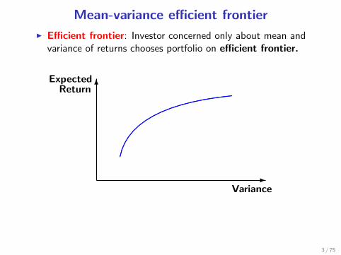
Mean-variance efficient frontier
I Efficient frontier: Investor concerned only about mean andvariance of returns chooses portfolio on efficient frontier.
-
6Expected
Return
Variance
..........................
........................
........................
........................
........................
.......................................................
.................................................................
...........................................................................
..................................................................................... ..............................................
3 / 75
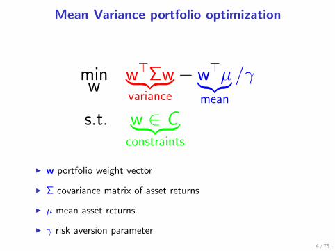
Mean Variance portfolio optimization
minw
w>Σw︸ ︷︷ ︸variance
− w>µ︸︷︷︸mean
/γ
s.t. w ∈ C︸ ︷︷ ︸constraints
I w portfolio weight vector
I Σ covariance matrix of asset returns
I µ mean asset returns
I γ risk aversion parameter
4 / 75
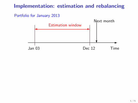
Implementation: estimation and rebalancing
-
-�Estimation window
?
Next month
Portfolio for January 2013
TimeJan 03 Dec 12
5 / 75
-
-�Estimation window
?
Next month
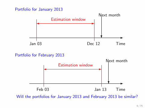
Portfolio for January 2013
TimeJan 03 Dec 12
-
-�Estimation window
?
Next month
TimeFeb 03 Jan 13
Portfolio for February 2013
Will the portfolios for January 2013 and February 2013 be similar?
6 / 75
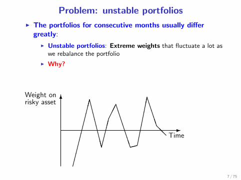
Problem: unstable portfolios
I The portfolios for consecutive months usually differgreatly:
I Unstable portfolios: Extreme weights that fluctuate a lot aswe rebalance the portfolio
I Why?
I Estimation error!!!
-
6Weight onrisky asset
Time
�����������CCCCCCCC��������BBBBBBB����������BBBBB@@
7 / 75
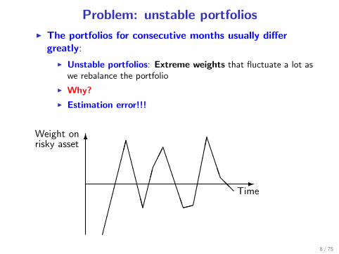
Problem: unstable portfolios
I The portfolios for consecutive months usually differgreatly:
I Unstable portfolios: Extreme weights that fluctuate a lot aswe rebalance the portfolio
I Why?
I Estimation error!!!
-
6Weight onrisky asset
Time
�����������CCCCCCCC��������BBBBBBB����������BBBBB@@
8 / 75
See also [Chopra and Ziemba, 1993] and [Broadie, 1993].

The 1/N paper
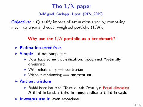
The 1/N paperDeMiguel, Garlappi, Uppal (RFS, 2009)
Objective: : Quantify impact of estimation error by comparingmean-variance and equal-weighted portfolio (1/N).
Why use the 1/N portfolio as a benchmark?
I Estimation-error free,I Simple but not simplistic:
I Does have some diversification, though not “optimally”diversified;
I With rebalancing =⇒ contrarian;I Without rebalancing =⇒ momentum.
I Ancient wisdom
I Rabbi Issac bar Aha (Talmud, 4th Century): Equal allocationA third in land, a third in merchandise, a third in cash.
I Investors use it, even nowadays.11 / 75
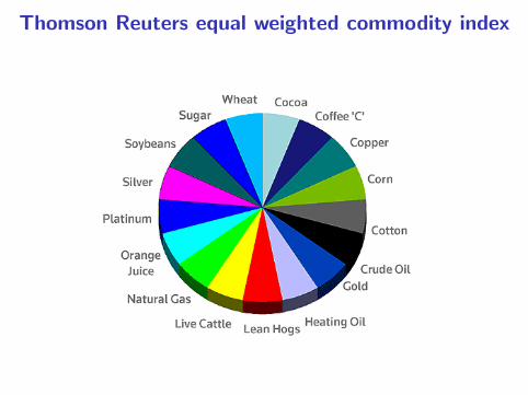
Thomson Reuters equal weighted commodity index
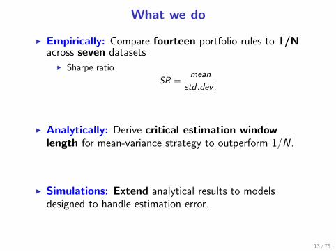
What we do
I Empirically: Compare fourteen portfolio rules to 1/Nacross seven datasets
I Sharpe ratio
SR =mean
std .dev .
I Analytically: Derive critical estimation windowlength for mean-variance strategy to outperform 1/N .
I Simulations: Extend analytical results to modelsdesigned to handle estimation error.
13 / 75
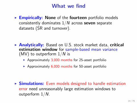
What we find
I Empirically: None of the fourteen portfolio modelsconsistently dominates 1/N across seven separatedatasets (SR and turnover).
I Analytically: Based on U.S. stock market data, criticalestimation window for sample-based mean variance(MV) to outperform 1/N is
I Approximately 3,000 months for 25-asset portfolio
I Approximately 6,000 months for 50-asset portfolio
I Simulations: Even models designed to handle estimationerror need unreasonably large estimation windows tooutperform 1/N .
14 / 75

Portfolios tested
I Bayesian portfolios
15 / 75
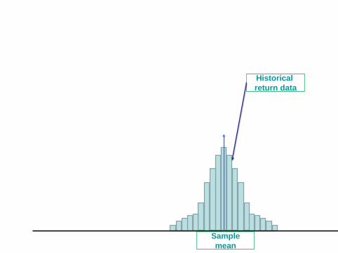
Historical return data
Sample mean
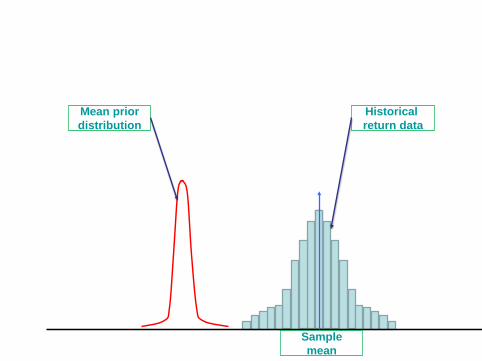
Historical return data
Sample mean
Mean prior distribution
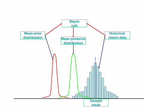
Historical return data
Sample mean
Mean prior distribution Mean posterior
distribution
Bayes rule
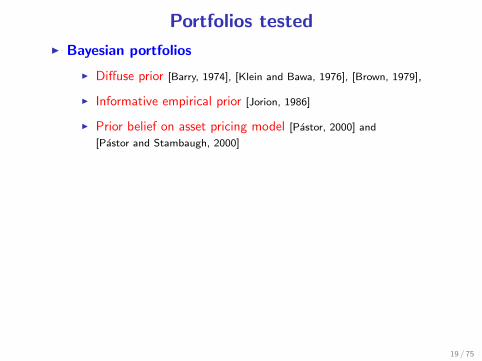
Portfolios tested
I Bayesian portfolios
I Diffuse prior [Barry, 1974], [Klein and Bawa, 1976], [Brown, 1979],
I Informative empirical prior [Jorion, 1986]
I Prior belief on asset pricing model [Pastor, 2000] and
[Pastor and Stambaugh, 2000]
I Portfolios with moment restrictions
I Portfolios subject to shortsale constraints
I Optimal combinations of portfolios
19 / 75
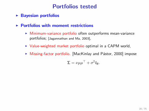
Portfolios tested
I Bayesian portfolios
I Portfolios with moment restrictions
I Minimum-variance portfolio often outperforms mean-varianceportfolios; [Jagannathan and Ma, 2003],
I Value-weighted market portfolio optimal in a CAPM world,
I Missing-factor portfolio. [MacKinlay and Pastor, 2000] impose
Σ = νµµ> + σ2IN .
I Portfolios subject to shortsale constraints
I Optimal combinations of portfolios
20 / 75
Portfolios tested
I Bayesian portfolios
I Portfolios with moment restrictions
I Portfolios subject to shortsale constraints[Jagannathan and Ma, 2003] show they perform well inpractice.
I Optimal combinations of portfolios
21 / 75
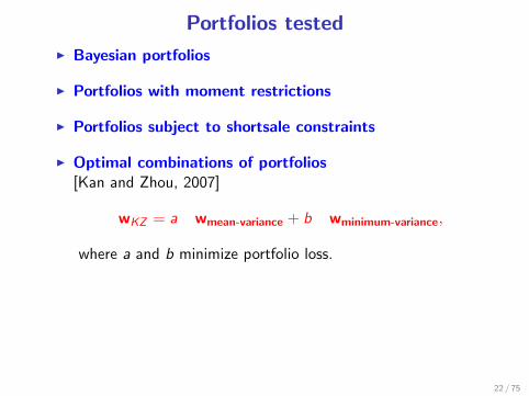
Portfolios tested
I Bayesian portfolios
I Portfolios with moment restrictions
I Portfolios subject to shortsale constraints
I Optimal combinations of portfolios[Kan and Zhou, 2007]
wKZ = a wmean-variance + b wminimum-variance,
where a and b minimize portfolio loss.
22 / 75
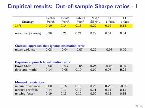
Empirical results: Out-of-sample Sharpe ratios - I
Sector Indust. Inter’l Mkt/ FF FFStrategy Portf. Portf. Portf. SB/HL 1-fact. 4-fact.
1/N 0.19 0.14 0.13 0.22 0.16 0.18
mean var (in sample) 0.38 0.21 0.21 0.29 0.51 0.54
Classical approach that ignores estimation errormean variance 0.08 -0.04 -0.07 0.22 -0.07 0.00
Bayesian approach to estimation errorBayes Stein 0.08 -0.03 -0.05 0.25 -0.06 0.00data and model 0.14 -0.05 0.10 0.02 0.07 0.24
Moment restrictionsminimun variance 0.08 0.16 0.15 0.25 0.28 -0.02market portfolio 0.14 0.11 0.12 0.11 0.11 0.11missing factor 0.19 0.13 0.12 0.06 0.15 0.15
23 / 75
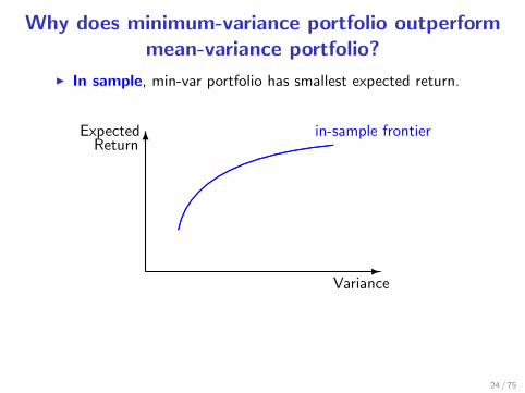
Why does minimum-variance portfolio outperformmean-variance portfolio?
I In sample, min-var portfolio has smallest expected return.
-
6Expected
Return
Variance
.........................
........................
.......................
.......................
........................
........................................................
..................................................................
.............................................................................
.......................................... .............................................in-sample frontier
24 / 75
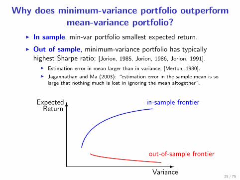
Why does minimum-variance portfolio outperformmean-variance portfolio?
I In sample, min-var portfolio smallest expected return.
I Out of sample, minimum-variance portfolio has typicallyhighest Sharpe ratio; [Jorion, 1985, Jorion, 1986, Jorion, 1991].
I Estimation error in mean larger than in variance; [Merton, 1980].
I Jagannathan and Ma (2003): “estimation error in the sample mean is solarge that nothing much is lost in ignoring the mean altogether”.
-
6Expected
Return
Variance
.........................
........................
.......................
.......................
........................
........................................................
..................................................................
.............................................................................
.......................................... .............................................
........ .......... .............. ................. .................... ....................... .......................... ............................. ................................ ................................... ...................................... ......................................... ............................................
in-sample frontier
out-of-sample frontier
25 / 75
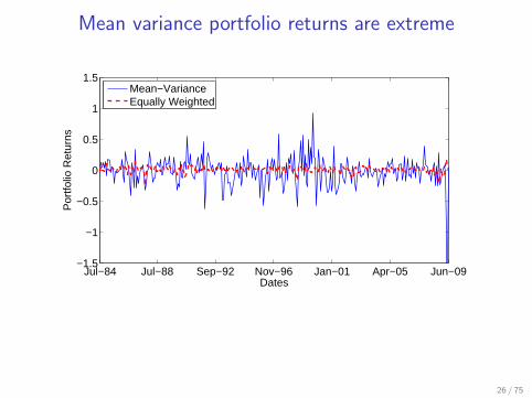
Mean variance portfolio returns are extreme
Jul−84 Jul−88 Sep−92 Nov−96 Jan−01 Apr−05 Jun−09−1.5
−1
−0.5
0
0.5
1
1.5
Dates
Por
tfolio
Ret
urns
Mean−VarianceEqually Weighted
26 / 75
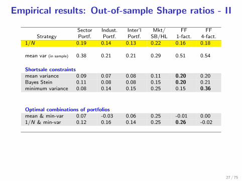
Empirical results: Out-of-sample Sharpe ratios - II
Sector Indust. Inter’l Mkt/ FF FFStrategy Portf. Portf. Portf. SB/HL 1-fact. 4-fact.
1/N 0.19 0.14 0.13 0.22 0.16 0.18
mean var (in sample) 0.38 0.21 0.21 0.29 0.51 0.54
Shortsale constraintsmean variance 0.09 0.07 0.08 0.11 0.20 0.20Bayes Stein 0.11 0.08 0.08 0.15 0.20 0.21minimum variance 0.08 0.14 0.15 0.25 0.15 0.36
Optimal combinations of portfoliosmean & min-var 0.07 -0.03 0.06 0.25 -0.01 0.001/N & min-var 0.12 0.16 0.14 0.25 0.26 -0.02
27 / 75
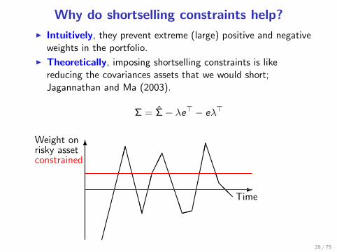
Why do shortselling constraints help?
I Intuitively, they prevent extreme (large) positive and negativeweights in the portfolio.
I Theoretically, imposing shortselling constraints is likereducing the covariances assets that we would short;Jagannathan and Ma (2003).
Σ = Σ− λe> − eλ>
-
6Weight onrisky assetconstrained
Time
�����������CCCCCCCC��������BBBBBBB����������BBBBB@@
28 / 75
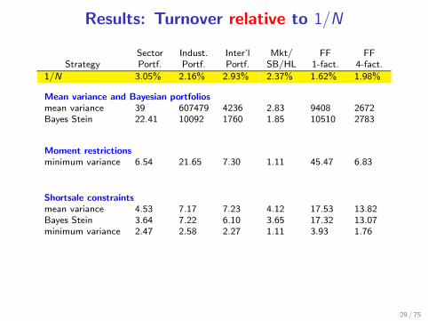
Results: Turnover relative to 1/N
Sector Indust. Inter’l Mkt/ FF FFStrategy Portf. Portf. Portf. SB/HL 1-fact. 4-fact.
1/N 3.05% 2.16% 2.93% 2.37% 1.62% 1.98%
Mean variance and Bayesian portfoliosmean variance 39 607479 4236 2.83 9408 2672Bayes Stein 22.41 10092 1760 1.85 10510 2783
Moment restrictionsminimum variance 6.54 21.65 7.30 1.11 45.47 6.83
Shortsale constraintsmean variance 4.53 7.17 7.23 4.12 17.53 13.82Bayes Stein 3.64 7.22 6.10 3.65 17.32 13.07minimum variance 2.47 2.58 2.27 1.11 3.93 1.76
29 / 75
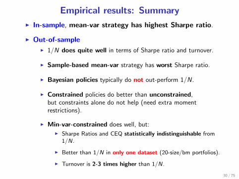
Empirical results: Summary
I In-sample, mean-var strategy has highest Sharpe ratio.
I Out-of-sample
I 1/N does quite well in terms of Sharpe ratio and turnover.
I Sample-based mean-var strategy has worst Sharpe ratio.
I Bayesian policies typically do not out-perform 1/N.
I Constrained policies do better than unconstrained,but constraints alone do not help (need extra momentrestrictions).
I Min-var-constrained does well, but:I Sharpe Ratios and CEQ statistically indistinguishable from
1/N.
I Better than 1/N in only one dataset (20-size/bm portfolios).
I Turnover is 2-3 times higher than 1/N.
30 / 75


Beating 1/N
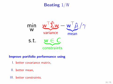
Beating 1/N
minw
w>Σw︸ ︷︷ ︸variance
− w>µ︸︷︷︸mean
/γ
s.t. w ∈ C︸ ︷︷ ︸constraints
Improve portfolio performance using
I. better covariance matrix,
II. better mean,
III. better constraints.
33 / 75
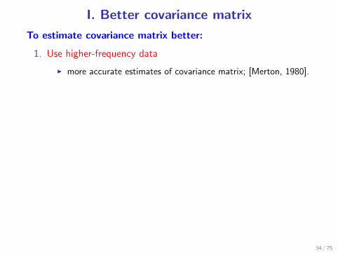
I. Better covariance matrix
To estimate covariance matrix better:
1. Use higher-frequency data
I more accurate estimates of covariance matrix; [Merton, 1980].
2. Use factor models
3. Use shrinkage estimators
34 / 75
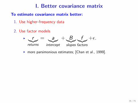
I. Better covariance matrix
To estimate covariance matrix better:
1. Use higher-frequency data
2. Use factor models
I r︸︷︷︸returns
= a︸︷︷︸intercept
+ B︸︷︷︸slopes
f︸︷︷︸factors
+ε.
I more parsimonious estimates; [Chan et al., 1999].
3. Use shrinkage estimators
35 / 75
I. Better covariance matrix
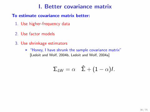
To estimate covariance matrix better:
1. Use higher-frequency data
2. Use factor models
3. Use shrinkage estimators
I “Honey, I have shrunk the sample covariance matrix”[Ledoit and Wolf, 2004b, Ledoit and Wolf, 2004a]
ΣLW = α Σ + (1− α)I .
36 / 75
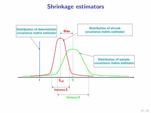
Shrinkage estimators
ΣI
Distribution of sample covariance matrix estimator
Distribution of shrunkcovariance matrix estimator
Distribution of deterministiccovariance matrix estimator Bias
Variance Σ
Variance Σ
ΣLW
37 / 75
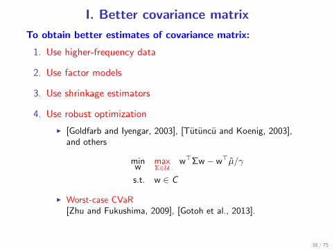
I. Better covariance matrix
To obtain better estimates of covariance matrix:
1. Use higher-frequency data
2. Use factor models
3. Use shrinkage estimators
4. Use robust optimization
I [Goldfarb and Iyengar, 2003], [Tutuncu and Koenig, 2003],and others
minw
maxΣ∈U
w>Σw− w>µ/γ
s.t. w ∈ C
I Worst-case CVaR[Zhu and Fukushima, 2009], [Gotoh et al., 2013].
5. Use robust estimation
38 / 75
I. Better covariance matrix
To obtain better estimates of covariance matrix:
1. Use higher-frequency data
2. Use factor models
3. Use shrinkage estimators
4. Use robust optimization
5. Use robust estimation
39 / 75
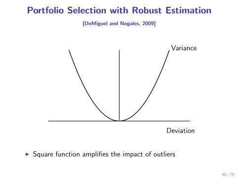
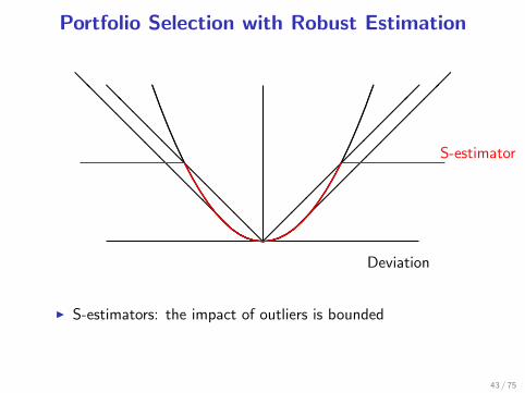
Portfolio Selection with Robust Estimation[DeMiguel and Nogales, 2009]
Deviation
.
..................................................
...............................................
...........................................
........................................
.....................................
..................................
..............................
...........................
........................
.....................
.................... ................... .................. ................. ................. ..............................................................................
........................
...........................
..............................
..................................
.....................................
........................................
...........................................
...............................................
..................................................
Variance
I Square function amplifies the impact of outliers
40 / 75
Portfolio Selection with Robust Estimation
Deviation
.
..................................................
...............................................
...........................................
........................................
.....................................
..................................
..............................
...........................
........................
.....................
.................... ................... .................. ................. ................. ..............................................................................
........................
...........................
..............................
..................................
.....................................
........................................
...........................................
...............................................
..................................................
�����������
@@
@@
@@@
@@
@@
Mad
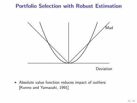
I Absolute value function reduces impact of outliers:[Konno and Yamazaki, 1991]
41 / 75
Portfolio Selection with Robust Estimation
Deviation
.
..................................................
...............................................
...........................................
........................................
.....................................
..................................
..............................
...........................
........................
.....................
....................
...................
.................. ................. ................. .....................................
....................
.....................
........................
...........................
..............................
..................................
.....................................
........................................
...........................................
...............................................
..................................................
�����������
@@
@@
@@@
@@
@@
...............
......
...................
.................. ................. ................. .....................................
....................@@
@@@
@@@
@@@
�����������
M-estimator
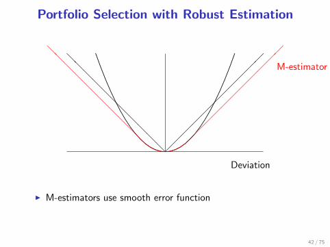
I M-estimators use smooth error function
42 / 75
Portfolio Selection with Robust Estimation
Deviation
.
..................................................
...............................................
...........................................
........................................
.....................................
..................................
..............................
...........................
........................
.....................
.................... ................... .................. ................. ................. ..............................................................................
........................
...........................
..............................
..................................
.....................................
........................................
...........................................
...............................................
..................................................
�����������
@@
@@
@@@
@@
@@
. .................... ................... .................. ................. ................. .........................................................
@@@
@@@
@@
@@@
�����������
.
....................................
.................................
..............................
...........................
.......................
.....................
.................... ................... .................. ................. ................. ..............................................................................
.......................
...........................
..............................
.................................
....................................
S-estimator
I S-estimators: the impact of outliers is bounded
43 / 75
II. Better mean
To obtain better estimates of mean:
1. Ignore means
2. Use Bayesian estimates
3. Use robust optimization
4. Use option-implied information
44 / 75
II. Better mean
To obtain better estimates of mean:
1. Ignore means
2. Use Bayesian estimates
3. Use robust optimization
4. Use option-implied information
45 / 75
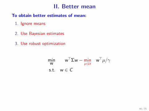
II. Better mean
To obtain better estimates of mean:
1. Ignore means
2. Use Bayesian estimates
3. Use robust optimization
minw
w>Σw−minµ∈U
w>µ/γ
s.t. w ∈ C
4. Use option-implied information
46 / 75
II. Better mean
To obtain better estimates of mean:
1. Ignore means
2. Use Bayesian estimates
3. Use robust optimization
4. Use option-implied information
47 / 75
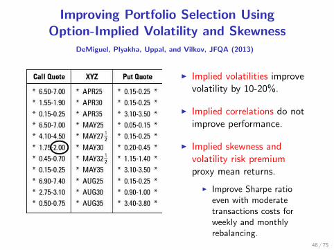
Improving Portfolio Selection UsingOption-Implied Volatility and Skewness
DeMiguel, Plyakha, Uppal, and Vilkov, JFQA (2013)
I Implied volatilities improvevolatility by 10-20%.
I Implied correlations do notimprove performance.
I Implied skewness andvolatility risk premiumproxy mean returns.
I Improve Sharpe ratioeven with moderatetransactions costs forweekly and monthlyrebalancing.
48 / 75
II. Better mean
To obtain better estimates of mean:
1. Ignore means
2. Use Bayesian estimates
3. Use robust optimization
4. Use option-implied information
5. Use stock return serial dependence
49 / 75
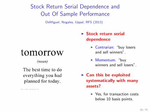
Stock Return Serial Dependence andOut Of Sample Performance
DeMiguel, Nogales, Uppal, RFS (2013)
I Stock return serialdependence
I Contrarian: “buy losersand sell winners”.
I Momentum: “buywinners and sell losers”.
I Can this be exploitedsystematically with manyassets?
I Yes, for transaction costsbelow 10 basis points.
50 / 75
II. Better mean
To obtain better estimates of mean:
1. Ignore historical means
2. Use Bayesian estimates
3. Use robust optimization
4. Use option-implied information
5. Use stock return serial dependence
6. Exploit anomalies
51 / 75
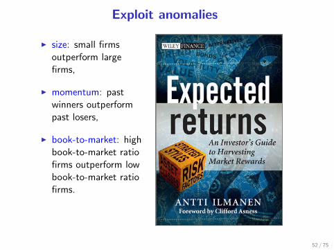
Exploit anomalies
I size: small firmsoutperform largefirms,
I momentum: pastwinners outperformpast losers,
I book-to-market: highbook-to-market ratiofirms outperform lowbook-to-market ratiofirms.
52 / 75
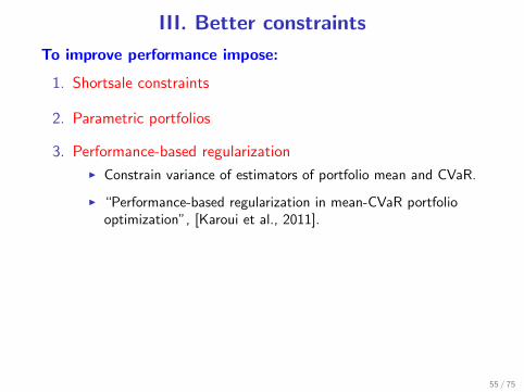
III. Better constraints
To improve performance impose:
1. Shortsale constraints
2. Parametric portfolios
3. Performance-based regularization
4. Norm constraints
53 / 75
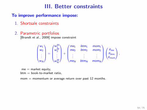
III. Better constraints
To improve performance impose:
1. Shortsale constraints
2. Parametric portfolios[Brandt et al., 2009] impose constraint
w1
w2
...wN
=
wM
1wM
2...
wMN
+
me1 btm1 mom1
me2 btm2 mom2
......
...meN btmN momN
θme
θbtmθmom
,
me = market equity,btm = book-to-market ratio,
mom = momentum or average return over past 12 months.
3. Performance-based regularization
4. Norm constraints
54 / 75
III. Better constraints
To improve performance impose:
1. Shortsale constraints
2. Parametric portfolios
3. Performance-based regularization
I Constrain variance of estimators of portfolio mean and CVaR.
I “Performance-based regularization in mean-CVaR portfoliooptimization”, [Karoui et al., 2011].
4. Norm constraints
55 / 75
III. Better constraints
To improve performance impose:
1. Shortsale constraints
2. Parametric portfolios
3. Performance-based regularization
4. Norm constraints
56 / 75
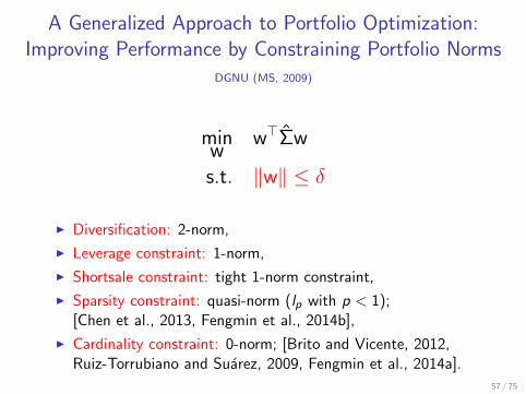
A Generalized Approach to Portfolio Optimization:Improving Performance by Constraining Portfolio Norms
DGNU (MS, 2009)
minw
w>Σw
s.t. ‖w‖ ≤ δ
I Diversification: 2-norm,
I Leverage constraint: 1-norm,
I Shortsale constraint: tight 1-norm constraint,
I Sparsity constraint: quasi-norm (lp with p < 1);[Chen et al., 2013, Fengmin et al., 2014b],
I Cardinality constraint: 0-norm; [Brito and Vicente, 2012,Ruiz-Torrubiano and Suarez, 2009, Fengmin et al., 2014a].
57 / 75


Help wanted
I Optimization can make a difference in portfolio selection.
I Research opportunities
I Integer variables
I Multistage optimization
I Calibration, calibration, calibration:
59 / 75
Help wanted
I Optimization can make a difference in portfolio selection.
I Research opportunities
I Integer variables
I VaR:
[Gaivoronski and Pflug, 2005], [Benati and Rizzi, 2007],Vera and Zuluaga (2013),
I fixed costs and cardinality constraints.
I Multistage optimization
I Calibration, calibration, calibration:
60 / 75
Help wanted
I Optimization can make a difference in portfolio selection.
I Research opportunities
I Integer variables
I Multistage optimization
I return predictability,
I transaction costs,
I Mei, D., Nogales, (2013), “Multiperiod Portfolio Optimizationwith General Transaction Costs”.
I Calibration, calibration, calibration:
61 / 75
Help wanted
I Optimization can make a difference in portfolio selection.
I Research opportunities
I Integer variables
I Multistage optimization
I Calibration, calibration, calibration:
62 / 75
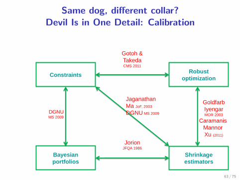
Same dog, different collar?Devil Is in One Detail: Calibration
Constraints Robust
optimization
Bayesian
portfolios
Shrinkage
estimators
Gotoh &
Takeda CMS 2011
DGNU MS 2009
Goldfarb
Iyengar MOR 2003
Caramanis
Mannor
Xu (2011)
Jorion JFQA 1986
Jaganathan
Ma JoF, 2003
DGNU MS 2009
63 / 75
Help wanted
I Optimization can make a difference in portfolio selection.
I Research opportunities
I Integer variablesI Multistage optimizationI Calibration, calibration, calibration
I “Size Matters: Optimal Calibration of Shrinkage Estimatorsfor Portfolio Selection”, [Martin-Utrera, D., Nogales, 2013],
I choose criterion carefully, get nonparametric.I Martin-Utrera, D., Nogales, JFQA (2014), “Parameter
Uncertainty in Multiperiod Portfolio Optimization withTransaction Costs”.
I Statistics/big data/real-time estimation and optimization:I stock return prediction: [Welch and Goyal, 2008] show that 15
predictors from the literature fail out of sample, and[Rapach et al., 2010] show that combining forecasts helps.
I hedge fund replication: [Roncalli and Weisang, 2011] showthat l1 regularization helps when replicating hedge fundreturns using 12 factors.
I high-frequency trading.
64 / 75
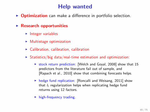
Help wanted
I Optimization can make a difference in portfolio selection.
I Research opportunities
I Integer variables
I Multistage optimization
I Calibration, calibration, calibration
I Statistics/big data/real-time estimation and optimization:
I stock return prediction: [Welch and Goyal, 2008] show that 15predictors from the literature fail out of sample, and[Rapach et al., 2010] show that combining forecasts helps.
I hedge fund replication: [Roncalli and Weisang, 2011] showthat l1 regularization helps when replicating hedge fundreturns using 12 factors.
I high-frequency trading.
65 / 75

High frequency trading
66 / 75
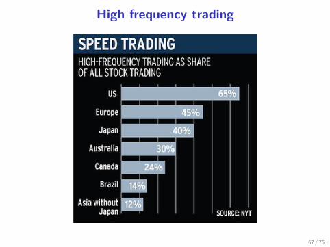
High frequency trading
67 / 75

High frequency trading
68 / 75

Thank you
Victor DeMiguelhttp://www.london.edu/avmiguel/
69 / 75
Barry, C. B. (1974).
Portfolio analysis under uncertain means, variances, and covariances.
Journal of Finance, 29(2):515–22.
Benati, S. and Rizzi, R. (2007).
A mixed integer linear programming formulation of the optimal mean/value-at-risk portfolio problem.
European Journal of Operational Research, 176(1):423–434.
Brandt, M. W., Santa-Clara, P., and Valkanov, R. (2009).
Parametric Portfolio Policies: Exploiting Characteristics in the Cross-Section of Equity Returns.
Review of Financial Studies, 22(9):3411–3447.
Brito, R. and Vicente, L. (2012).
Efficient cardinality/mean-variance portfolios.
Universidade de Coimbra working paper.
Broadie, M. (1993).
Computing efficient frontiers using estimated parameters.
Annals of Operations Research, 45:21–58.
Brown, S. (1979).
the effect of estimation risk on capital market equilibrium.
Journal of Financial and Quantitative Analysis, 14(2):215–220.
Chan, L. K. C., Karceski, J., and Lakonishok, J. (1999).
On portfolio optimization: Forecasting covariances and choosing the risk model.
Review of Financial Studies, 12(5):937–974.
Chen, C., Li, X., Tolman, C., Wang, S., and Ye, Y. (2013).
70 / 75
Sparse portfolio selection via quasi-norm regularization.
arXiv preprint arXiv:1312.6350.
Chopra, V. K. and Ziemba, W. T. (1993).
The effect of errors in means, variances, and covariances on optimal portfolio choice.
Journal of Portfolio Management, 19(2):6–11.
DeMiguel, V., Garlappi, L., Nogales, F., and Uppal, R. (2009a).
A Generalized Approach to Portfolio Optimization: Improving Performance By Constraining PortfolioNorms.
Management Science, 55(5):798–812.
DeMiguel, V., Garlappi, L., and Uppal, R. (2009b).
Optimal versus naive diversification: How inefficient is the 1/n portfolio strategy?
Review of Financial Studies, 22(5):1915–1953.
DeMiguel, V., Martın Utrera, A., and Nogales, F. J. (2013a).
Parameter uncertainty in multiperiod portfolio optimization with transaction costs.
Forthcoming in Journal of Financial and Quantitative Analysis.
DeMiguel, V., Martin-Utrera, A., and Nogales, F. J. (2013b).
Size matters: Optimal calibration of shrinkage estimators for portfolio selection.
Journal of Banking & Finance, 37(8):3018–3034.
DeMiguel, V., Mei, X., and Nogales, F. J. (2013c).
Multiperiod portfolio optimization with general transaction costs.
London Business School working paper.
DeMiguel, V., Nogales, F., and Uppal, R. (2014).
Stock return serial dependence and out-of-sample portfolio performance.
71 / 75
The Review of Financial Studies, 27(4):1031–1073.
DeMiguel, V. and Nogales, F. J. (2009).
Portfolio selection with robust estimation.
Operations Research, 57(3):560–577.
DeMiguel, V., Plyakha, Y., Uppal, R., and Vilkov, G. (2013d).
Improving portfolio selection using option-implied volatility and skewness.
Journal of Financial and Quantitative Analysis, 48(6):1813–1845.
Fengmin, X., Lu, Z., and Xu, Z. (2014a).
An efficient optimization approach for cardinality constrained index tracking problems.
Fengmin, X., Xu, Z., and Xue, H. (2014b).
Sparse index tracking: An l1/2 regularization based model and solution.
Gaivoronski, A. A. and Pflug, G. (2005).
Value-at-risk in portfolio optimization: properties and computational approach.
Journal of Risk, 7(2):1–31.
Goldfarb, D. and Iyengar, G. (2003).
Robust portfolio selection problems.
Mathematics of Operations Research, 28(1):1–38.
Gotoh, J.-Y., Shinozaki, K., and Takeda, A. (2013).
Robust portfolio techniques for mitigating the fragility of cvar minimization and generalization to coherentrisk measures.
Quantitative Finance, (ahead-of-print):1–15.
Ilmanen, A. (2011).
72 / 75
Expected Returns: An Investor’s Guide to Harvesting Market Rewards.
Wiley.
Jagannathan, R. and Ma, T. (2003).
Risk reduction in large portfolios: Why imposing the wrong constraints helps.
Journal of Finance, 58(4):1651–1684.
Jorion, P. (1985).
International portfolio diversification with estimation risk.
Journal of Business, 58:259–278.
Jorion, P. (1986).
Bayes-stein estimation for portfolio analysis.
Journal of Financial and Quantitative Analysis, 21(3):279–292.
Jorion, P. (1991).
Bayesian and capm estimators of the means: Implications for portfolio selection.
Journal of Banking and Finance, 15(3):717–727.
Kan, R. and Zhou, G. (2007).
Optimal portfolio choice with parameter uncertainty.
Journal of Financial and Quantitative Analysis, 42(3):621–656.
Karoui, N. E., Lim, A. E., and Vahn, G.-Y. (2011).
Performance-based regularization in mean-cvar portfolio optimization.
London Business School working paper.
Klein, R. W. and Bawa, V. S. (1976).
The effect of estimation risk on optimal portfolio choice.
73 / 75
Journal of Financial Economics, 3(3):215–31.
Konno, H. and Yamazaki, H. (1991).
Mean-absolute deviation portfolio optimization model and its applications to tokyo stock market.
Management science, 37(5):519–531.
Ledoit, O. and Wolf, M. (2004a).
Honey, i shrunk the sample covariance matrix.
Journal of Portfolio Management, 30(4):110–119.
Ledoit, O. and Wolf, M. (2004b).
A well-conditioned estimator for large-dimensional covariance matrices.
Journal of Multivariate Analysis, 88:365–411.
MacKinlay, A. C. and Pastor, L. (2000).
Asset pricing models: Implications for expected returns and portfolio selection.
Review of Financial Studies, 13(4):883–916.
Merton, R. C. (1980).
On estimating the expected return on the market: An exploratory investigation.
Journal of Financial Economics, 8:323–361.
Pastor, L. (2000).
Portfolio selection and asset pricing models.
Journal of Finance, 55(1):179–223.
Pastor, L. and Stambaugh, R. F. (2000).
Comparing asset pricing models: An investment perspective.
Journal of Financial Economics, 56(3):335–81.
74 / 75
Rapach, D. E., Strauss, J. K., and Zhou, G. (2010).
Out-of-sample equity premium prediction: Combination forecasts and links to the real economy.
Review of Financial Studies, 23(2):821–862.
Roncalli, T. and Weisang, G. (2011).
Tracking problems, hedge fund replication, and alternative beta.
Journal of Financial Transformation, 31:19–29.
Ruiz-Torrubiano, R. and Suarez, A. (2009).
A hybrid optimization approach to index tracking.
Annals of Operations Research, 166(1):57–71.
Tutuncu, R. and Koenig, M. (2003).
Robust asset allocation.
Working Paper, Carnegie Mellon University.
Welch, I. and Goyal, A. (2008).
A comprehensive look at the empirical performance of equity premium prediction.
Review of Financial Studies, 21(4):1455–1508.
Zhu, S. and Fukushima, M. (2009).
Worst-case conditional value-at-risk with application to robust portfolio management.
Operations Research, 57(5):1155–1168.
75 / 75