Adam C. Kellerman1, Y. Y. Shprits1,3, T. Podladchikova4,A. Drozdov1, H. Zhu5, D. Kondrashov2

1. Department of Earth, Planetary, and Space Sciences, UCLA2. Department of Atmospheric and Ocean Sciences, UCLA3. GFZ German Research Centre for Geosciences, University of Potsdam, Germany4. Skolkovo Institute of Technology, Skolkovo, Russia5. University of Texas, Dallas

Data Assimilation, and Forecasting the near-Earth Radiation Environment

1. VERB2. GOES/Van Allen Probe data3. Data Assimilation4. Data Assimilative Forecasting with VERB5. A long-term reanalysis dataset

Presentation Outline

Versatile Electron Radiation Belt code

The VERB code models the global state and evolution of the Earth’s radiation belt electrons

What’s special about this code?

1. We operate in an invariant coordinate system, where radiation particles ‘live’2. The code is fast, and can be run on a personal computer due to its advanced, and

accurate, numerical architecture

Observations (data)

GOES 13 and 15:MagED and EPEAD: 10’s of keV to ~2 MeV

Van Allen Probe A & B:MagEIS: 10’s of keV to MeV

Coverage at GEO and through GTO

Solar Wind/Geomagnetic IndicesSWPC: 3-day forecast Kp index: SWPC: Ace data:

Data Assimilation

Individually, data and models may not accurately specify the environment

Model Data

Global estimate withsome error and bias

Sparse observation withsome error and bias

If we combine the model and data, we may obtain an estimate closer to the truth

Model Data

Global coverage with a smaller overall error and bias

Data Assimilation

Real time ACE solar wind (SWPC)

Real-time Van Allen Probe data

Real time GOES 13 and 15 data

Real time and forecast Kp (SWPC)

Adiabatic Coordinates/electron PSD VERB

Forecast radiation belt state

Data Assimilation

Nowcast radiation belt state

DataModelProcessProduct

Radiation Belt Forecast Framework

Global Radiation Belt Forecast

Data assimilation allows to account for hysteresis (bias) effects

Data are sparse, often missing, or have processing errors. There are many gaps

Reanalysis allows for reconstruction of the radiation belt fluxes, even when data are missing

Here we highlight the importance of GOES data for our forecast framework

Forecast solar wind data are limited

In order to test and validate model performance, a study of forecast performance using final data is required

http://rbm.epss.ucla.edu/realtime-forecast/

Robust During Data Outage

We have a 4-year dataset of radiation belt-electron reanalysiscurrently 2012-2016Will be extended back to 1995

Such a dataset can be useful for specifying the environment around a given spacecraft

Averaging over time, energy, and space can be accomplished for 100 keV to multi-MeV electrons

A Long-Term Global Dataset

1. Implemented a robust and fast data-assimilation method for VERB 2.0

2. Real-time radiation belt nowcasts and forecasts using data assimilation -running every 2 hours, begun in 2015 – SWPC & APL

3. A long-term dataset of globally reconstructed fluxes is available from 2012-2016. This will be extended back to 1995, and forward as more data are available

4. Forecast validation has been complete – a more accurate and advanced model will be released in the near future

Summary

Radiation is hazardous to satellite electronics & humans in space

Over 3,000 satellites; Supporting $25B/yr industry; Replacement cost: over $75B; GPS industry ~ $1 trillion

Electric-orbit raising ~6 month transition through the belts

Space radiation impacts polar flights (~7,000) (cost ~$0.1 M per flight) examples: NY -Tokyo; LA - Moscow; disruption of power grids, produces blackouts (up to $100M in losses)

A Carrington type storm (1859) may cause $0.6-2.6 trillion in damage

Space Weather Effects

Particle Motion

Bounce period for a particle on anequipotential field line. The integrablesingularity at the mirror points poses aproblem.

We use MPI-FORTRAN routines to trace particles at high precision in a realistic time-dependent magnetic field model, and compute I, t, and the dI/dr

We can use a change of variables

In this way, we can compute thebounce time using standard numericalapproaches at all points along thebounce orbit

Orlova and Shprits, [2011]

Particle Motion

Related to the second invariant J = 2pIHow do we compute thebounce-averaged gradient andcurvature drift velocity?

We compute I numerically in a realisticmagnetic field model, in order to match ourpredetermined grid in K.

We obtain I for the reference field line, aswell as Bm, alpha, and the gradient of I.

The location of the mirror point allows usto compute a time-dependent and MLT-dependent loss cone.

Last, we also compute the E x B drift usinga Volland-Stern E-field.

The Radiation BeltsAdiabatic invariants are conserved forelectron energies of 100’s of keV toseveral MeV, which form the electronradiation belts.

Electron radiation belts typically consistof an inner and an outer belt

‘Slot’ region caused by scattering ofparticles, principally plasmaspheric hiss[Lyons and Thorne, 1973; Abel andThorne, 1998]

The inner region is very stable andparticles have a very long lifetime ~years

The outer region is much more dynamicand is a topic of ongoing study

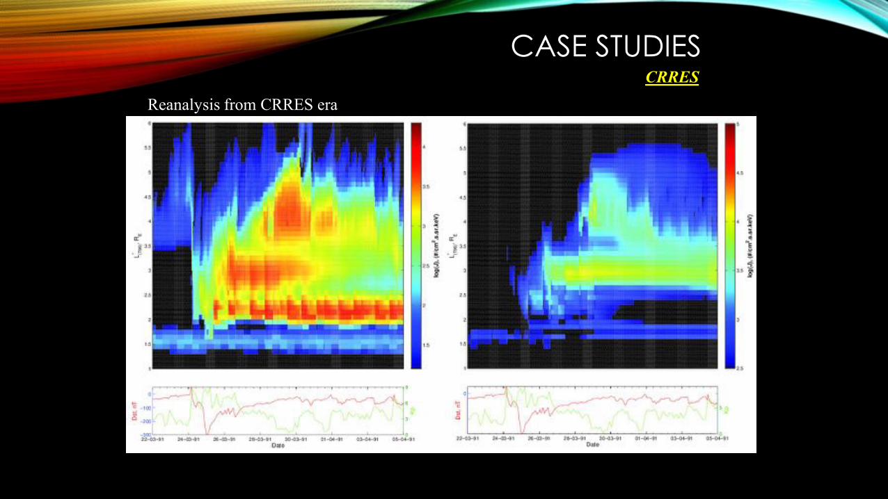
CASE STUDIESCRRES

Reanalysis from CRRES era

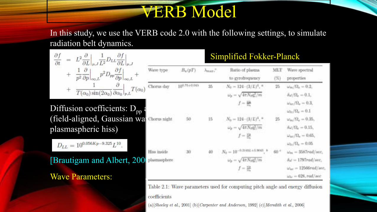
In this study, we use the VERB code 2.0 with the following settings, to simulate radiation belt dynamics.

Simplified Fokker-Planck equation. (L,m,J) & (L,p,a)

Diffusion coefficients: Dpp and Daa [Shprits et al., 2006b; Summers, 2005] (field-aligned, Gaussian wave-power spectrum for night and day chorus, and plasmaspheric hiss)

Wave Parameters:

[Brautigam and Albert, 2000]

VERB Model

Boundary conditions are as indicated to right, except for outer boundary. We useL = 6 and update outer boundary PSD from reanalysis from previous time step.

Wave Parameters:

[Subbotin and Shprits, 2009]

We use a simplified single grid. (L, m, a), which is correct within wave parameterization error ~30%, provided the grid is large enough, time step is small enough, and we use a logarithmic energy grid.

VERB Model

Real time ACE solar wind

Real-time Van Allen Probes

Real time GOES 13 and 15

Radiation Belt Forecast Framework

Real time and forecast Kp

L* and PSD (T89)

Nowcast PSD VERB

Forecast radiation belt stateKalman Filter

Nowcast radiation belt state

DataModelProcessProduct

http://rbm.epss.ucla.edu/realtime-forecast/

Recent example of radiation belt forecast fluxes at 1 MeV

The forecast runs every 2 hours automatically, and the most recent forecast figure is shown at the following web address

http://rbm.epss.ucla.edu/realtime-forecast/

Reanalysis and Forecasting

Forecast Performance

Kellerman et al., [2016], Space Weather – in preparation

Forecast PerformanceThe B-field model is important!

March, 20131 21

Diffusion Coefficients

Hui Zhu - Friday 4pm – GEM, QARBM

Diffusion Coefficients

DA BACKUP

X: State vector, PSD (c/(cm.MeV))3

M: Model matrix (VERB code)P: State error covariance matrixQ: Model covariance matrix.y: PSD measurementsK: Kalman GainR: Measurement error

|1 ttf XMX

tTtttf QMPMP 1

)( fttfa XyKXX 1)( tfft RPPK

fta PKIP )(

Forecast Step: Update Step

Forecast Update

Kalman Filter

We set out to minimize:

PSD at fixed L*, m, and K.

PSD1 is the reference or gold standardcf is a calibration coefficient

Find cf that minimizes the mean DPSD for each fixed invariant pair

Use the weighted mean of cf for all L* and K conjunctions to correct each energy channel, and estimate the bias. The width of the distribution gives an estimate of the error between the two spacecraft.

)/()(2 121221 PSDPSDcPSDPSDcPSD ff D

ERL 1.0* D min5Dt

Observational error and bias

Observational error and bias

Vampola,and Korth [1992] In this study, we focus on two enhancements in electron flux observed during the same storm

Background March 1991

We include 5 Spacecraft:

CRRES - HAEO

Akebono - LEO

GPSns18 - MEO

GEO1989 - GEO

GEO1990 - GEO

Observations

CRRES was located pre-midnight at 23.5 MLT and near L* = 4 during this period

a) Flux increases across all energies early on March 26

b) Adiabatic above ~0.4 MeV, and non-adiabatic below.

c) Evidence of dipolarization in Bz

Evidence of a particle injection.

The Third Radiation Belt

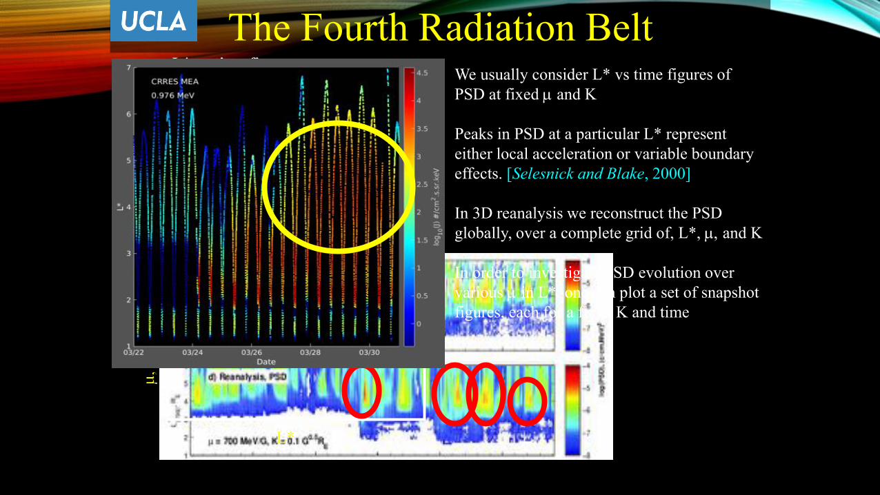
We usually consider L* vs time figures of PSD at fixed m and K

Peaks in PSD at a particular L* represent either local acceleration or variable boundary effects. [Selesnick and Blake, 2000]

In 3D reanalysis we reconstruct the PSD globally, over a complete grid of, L*, m, and K

In order to investigate PSD evolution over various m in L*, one can plot a set of snapshot figures, each for a fixed K and time

Fixed Invariant m and KColor coding is PSD

Time, days

Fixed time and K

L*

Snapshot analysis

L* vs time figures

The Fourth Radiation Belt

Each panel represents a snapshot, indicated by the blue dashed lines in panel (k)

1) Rapid loss during the main phase

2) The appearance of a third radiation belt

3) Growing peaks in PSD to form a fourth belt

The growing peaks in PSD indicate that the fourth belt was created by local acceleration.

Kellerman et al., [2014], JGR

PSD Analysis

There are 4 mechanisms that resulted in the observed four-zone structure

1. Prompt injection2. Secondary injection3. Losses/outward radial diffusion4. Local acceleration

13 MeV

1 2 34

B1

B4

B3

B2

1 MeV

4-Zone Structure

Van Allen Probe and GOES data, now including losses to the magnetopause based on the last-closed-drift shell (LCDS)

Invariant coordinates are based on T89, T04s and TS07D-1A

The LCDS is currently based on T04s

The dataset spans Oct 2012 – Oct 2016

Reanalysis dataset including LCDS

LCDS work with Steve Morley and Jay Albert (LANL/AFRL)

TS07D model work with Grant Stephens and Misha Sitnov (APL)

Integration into IRBEM with Paul O’Brien (Aerospace) and Sebastian Bourdarie(ONERA)

LRadial Diffusion Model

34567

-1

-0.5

0

0.5

L

Hourly averaged CRRES observations

m=700 MeV G-1 K=0.11 G0.5 RE34567

-1

-0.5

0

0.5

0 10 20 30 40 5002468

Time, days

Kp

[Shprits et al., 2007]

1D Data AssimilationFirst application to our 1D-radial diffusion model -f/t

L

Radial Diffusion Model with t = 1/Kp

4567

-1-0.500.5

L

Sparce data, Radial Diffusion Model with t = 1/Kp

m=700 MeV G-1 K=0.11 G0.5 RE4567

-1-0.500.5

L

Radial Diffusion Model with t = 5/Kp

4567

-1-0.500.5

L

Radial Diffusion Model with t = 5/Kp, data t = 1/Kp

4567

-1-0.500.5

0 10 20 30 40 500

5

Time, days

Kp

204060

1D Data AssimilationFirst application to our 1D-radial diffusion model -f/t

[Shprits et al., 2007]

Persistent peaks in PSD and positive innovation indicate that in addition to the radial diffusion there is another acceleration mechanism present in the inner magnetosphere.

Negative innovation at the outer L-shells may indicate an additional loss mechanism.

1D Data Assimilation

)( fttfa XyKXX

ftt

ft XMX 11 f

tEttf

t XMMX 111 a

2D Data Assimilation