Data acquisition for an electric mining shovel

pose estimator

Sebastiaan van der Tas

DCT 2008.025

Jan 2008

i

Contents

1 Introduction 11.1 Electric mining shovels . . . . . . . . . . . . . . . . . . . . . . . . . . . . . . . . . 11.2 Pose estimator . . . . . . . . . . . . . . . . . . . . . . . . . . . . . . . . . . . . . 21.3 Report overview . . . . . . . . . . . . . . . . . . . . . . . . . . . . . . . . . . . . 3

2 The Global Positioning System 42.1 GPS . . . . . . . . . . . . . . . . . . . . . . . . . . . . . . . . . . . . . . . . . . . 4

2.1.1 Segmentation of the GPS . . . . . . . . . . . . . . . . . . . . . . . . . . . 42.1.2 Calculation of position . . . . . . . . . . . . . . . . . . . . . . . . . . . . . 42.1.3 Carrier Phase GPS . . . . . . . . . . . . . . . . . . . . . . . . . . . . . . . 62.1.4 Differential GPS . . . . . . . . . . . . . . . . . . . . . . . . . . . . . . . . 6

2.2 Setting up an RTK differential GPS system . . . . . . . . . . . . . . . . . . . . . 72.2.1 Setting up an RTK base station using RTCM RTK messages (Z-Max) . . 82.2.2 Setting up an RTK remote station (rover) using RTCM RTK messages

(Z-Extreme) . . . . . . . . . . . . . . . . . . . . . . . . . . . . . . . . . . . 112.3 Transformations to the position data . . . . . . . . . . . . . . . . . . . . . . . . . 11

2.3.1 Transformation from geodetic coordinates to ECEF rectangular coordinates 122.3.2 Transformation from ECEF to tangent plane . . . . . . . . . . . . . . . . 13

2.4 Results . . . . . . . . . . . . . . . . . . . . . . . . . . . . . . . . . . . . . . . . . . 14

3 IMU 173.1 Specifications and position . . . . . . . . . . . . . . . . . . . . . . . . . . . . . . . 173.2 Results . . . . . . . . . . . . . . . . . . . . . . . . . . . . . . . . . . . . . . . . . . 18

3.2.1 Gyros . . . . . . . . . . . . . . . . . . . . . . . . . . . . . . . . . . . . . . 183.2.2 Accelerometers . . . . . . . . . . . . . . . . . . . . . . . . . . . . . . . . . 183.2.3 Noise from crowd drive . . . . . . . . . . . . . . . . . . . . . . . . . . . . 213.2.4 Noise from hoist drive . . . . . . . . . . . . . . . . . . . . . . . . . . . . . 24

4 Inclinometer 274.1 Specifications and position . . . . . . . . . . . . . . . . . . . . . . . . . . . . . . . 274.2 Results . . . . . . . . . . . . . . . . . . . . . . . . . . . . . . . . . . . . . . . . . . 27

5 Tachometers 315.1 Installation of Tachometers . . . . . . . . . . . . . . . . . . . . . . . . . . . . . . 315.2 Measurements of tachometers . . . . . . . . . . . . . . . . . . . . . . . . . . . . . 32

5.2.1 Swing motor . . . . . . . . . . . . . . . . . . . . . . . . . . . . . . . . . . 325.2.2 Crowd motor . . . . . . . . . . . . . . . . . . . . . . . . . . . . . . . . . . 335.2.3 Hoist motor . . . . . . . . . . . . . . . . . . . . . . . . . . . . . . . . . . . 34

ii

6 Conclusion 35

A List of abbreviations 36A.1 List of Abbreviations . . . . . . . . . . . . . . . . . . . . . . . . . . . . . . . . . . 36

B RTCM messages 37

C NMEA messages 39

iii

List of Tables

3.1 Mean output and standard deviation of the gyros. . . . . . . . . . . . . . . . . . 183.2 Mean output and standard deviation of the accelerometers. . . . . . . . . . . . . 183.3 Mean output and standard deviation of the gyros and accelerometers with and

without activation of the hoist drive. . . . . . . . . . . . . . . . . . . . . . . . . . 24

B.1 Message type 3 and first part of message types 18, 19, 20 and 21 . . . . . . . . . 37B.2 Remaining for message type 18 and 20. . . . . . . . . . . . . . . . . . . . . . . . . 38B.3 Remaining for message type 19 and 21. . . . . . . . . . . . . . . . . . . . . . . . . 38

C.1 Contents of NMEA position response messages (POS) from the rover. . . . . . . 39C.2 Contents of NMEA position response messages (GGA) from the rover. . . . . . . 40

iv

v

Chapter 1

Introduction

1.1 Electric mining shovels

Electric mining shovels (EMS) are electro-mechanical excavators which are used in open-cutmining sites for loading large haul trucks. They are mostly used for coal, copper, iron ore, oilsands and other minerals. A P&H 2100 BLE shovel is used by CRC Mining at Bracalba Quarryto develop shovel automation technologies in partnership with P&H.Figure (1.1) shows a P&H class electric mining shovel which consists of a base (crawler tracks)which stands on the ground and on that base is the machinery house which can rotate with respectto the base. The machinery house contains the main electrical components, the operator’s caband it supports the boom. The lower end of the boom is pin jointed to the machinery houseand the upper end is supported by the gantry ropes. Attached to the boom is the saddle whichsupports the handle but allows the handle to pivot and translate in the plane of the boom. Thedipper is mounted rigidly at the end of the handle. The hoist ropes are attached to the dippervia the bail which can pivot around the bail pin. At the bottom of the dipper is the dipper doorwhich can be opened in order to dump the material into the haul truck.

While digging the EMS works in an operating cycle that consists of three phases. In thefirst phase (dig phase) the dipper gets filled with a digging pass through the bench. A benchis the vertical face of the material that has to be excavated. When the dipper is full, a loadedswing to the dump position will follow and the material will be dumped when the dipper dooris opened. This is called the swing-to-dump phase. After dumping the material into the haultruck the return phase starts wherein the empty dipper is returned from the dump position tothe position at which the next dig can begin.

After loading a number of trucks from one position, the EMS will use its crawler tracks topropel. This is done to the position to efficiently load subsequent trucks.During the dig phase the shovel makes use of three actuators: swing drive, hoist drive and crowd

drive. The swing drive rotates the machine house with respect to the crawler tracks. It consistsof a DC motor and a transmission. On the 2100 BLE, it is located in the front of the machinehouse. Larger shovels can have up to three swing drive units.The hoist drive hoists or lowers the dipper (and handle). In the machine house a DC motordrives a drum on which the hoist ropes are wound. From the drum the hoist ropes go aroundthe boom point sheaves and are attached to the bail.The crowd drive moves the handle forwards or backwards and is driven by a DC motor attachedto the boom just below the pinion. This motor drives a belt which drives a rack and pinionarrangement. The belt slips at a certain torque so the handle will have a maximum force

1

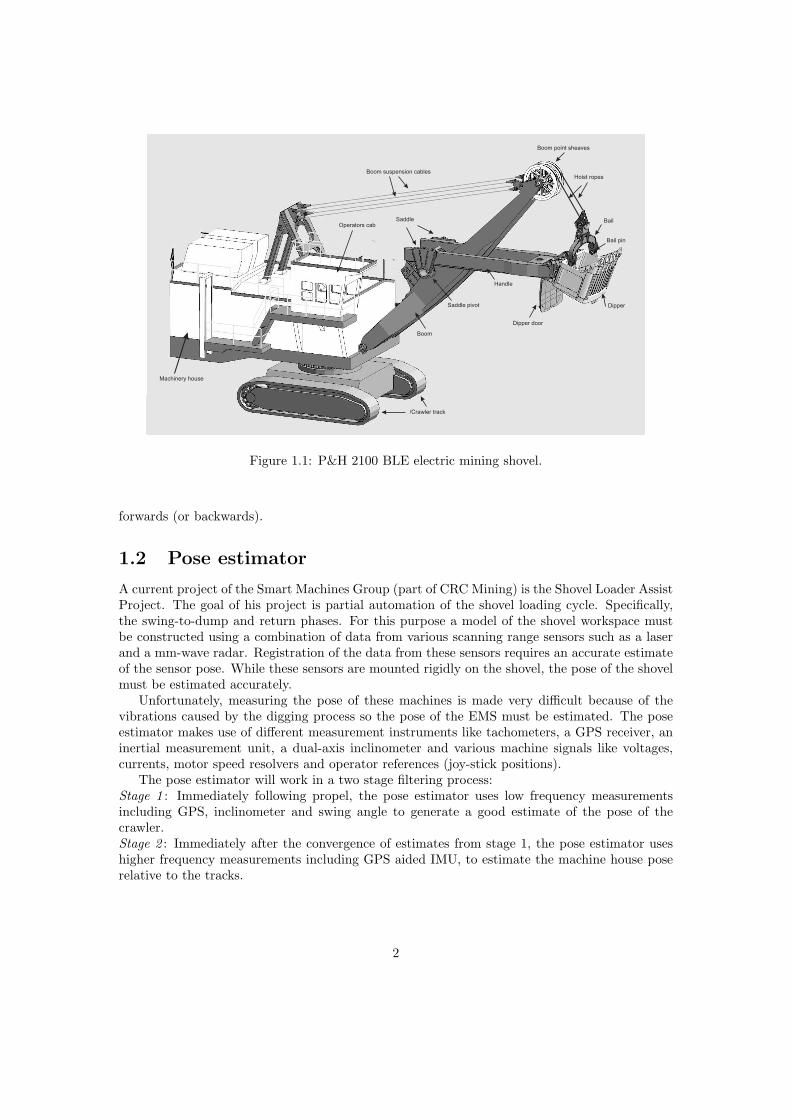
Figure 1.1: P&H 2100 BLE electric mining shovel.

forwards (or backwards).

1.2 Pose estimator

A current project of the Smart Machines Group (part of CRC Mining) is the Shovel Loader AssistProject. The goal of his project is partial automation of the shovel loading cycle. Specifically,the swing-to-dump and return phases. For this purpose a model of the shovel workspace mustbe constructed using a combination of data from various scanning range sensors such as a laserand a mm-wave radar. Registration of the data from these sensors requires an accurate estimateof the sensor pose. While these sensors are mounted rigidly on the shovel, the pose of the shovelmust be estimated accurately.

Unfortunately, measuring the pose of these machines is made very difficult because of thevibrations caused by the digging process so the pose of the EMS must be estimated. The poseestimator makes use of different measurement instruments like tachometers, a GPS receiver, aninertial measurement unit, a dual-axis inclinometer and various machine signals like voltages,currents, motor speed resolvers and operator references (joy-stick positions).

The pose estimator will work in a two stage filtering process:Stage 1 : Immediately following propel, the pose estimator uses low frequency measurementsincluding GPS, inclinometer and swing angle to generate a good estimate of the pose of thecrawler.Stage 2 : Immediately after the convergence of estimates from stage 1, the pose estimator useshigher frequency measurements including GPS aided IMU, to estimate the machine house poserelative to the tracks.

2

1.3 Report overview

• Installation and commissioning of sensor suite for pose estimator, including:

– Installation, manual and results of an RTK GPS base station & rover are explainedin Chapter 2.

– Chapter 3 deals with the installation and results of a 6 axis IMU, mounted in themachine house.

– In Chapter 4 the results of a dual axis inclinometer are explained.

– Chapter 5 gives the results of the installed tachometers.

• In all chapters the data collection and sanity check in preparation for application to EMSpose estimation will be discussed.

3

Chapter 2

The Global Positioning System

2.1 GPS

2.1.1 Segmentation of the GPS

The Global Positioning System is a satellite-based radio-navigation system which works in allweather conditions and at all locations in the world. It consists of three major segments: space,control and user [1].

The space segment originally consists of 24 Satellite Vehicles (SVs) which orbit the earth insix orbital planes. Four SVs are in each plane and orbit the earth in 11 hours and 58 minutes.The six planes are equally spaced around the equator which results in a 60◦ angle separation andhave a 55◦ inclination relative to the equator. The radius of the orbit is approximately 26600km. Figure 2.1 shows the constellation of the 24 GPS satellites (black triangles) orbiting theearth. The red dotted curves show the orbits of the satellites, one of the curves is a continuousline making it easier to observe the orbit. This constellation ensures that at least four satellitesare in sight at each location on the earth. Nowadays the constellation consists of 31 satellites toimprove reliability and availability of the system when multiple satellites fail.

Every SV emits a coded radio signal which will be sent to the receiver of the user. Thereceiver consists of an antenna and a receiver-processor which decodes the signal and computesthe position, velocity and precise timing information. The communications are in one direction,from the satellites to the receiver which operates passively. This makes it possible to provideservice to an unlimited number of receivers.

The information sent by the SVs contains time and position information. This informationmust be very accurate to obtain precise positions on the globe. Therefore this information mustbe checked and updated quiet often. The control segment is responsible for this part of the GPS.The master control station checks the positions, health and time offset of the SVs and makescorrections for it. These corrections will be sent to the SVs by antenna stations around theworld.

2.1.2 Calculation of position

From the information sent by the SVs the GPS receiver can calculate its position. This infor-mation consists of the identity number of the SV, the exact time the information was sent andinformation of its position, or ephemeris, on that very moment. Ephemeris means the position ofthe satellite in space and can be calculated with a number of equations and the parameters sent

4

−2

worldPrimary meridianEquatororbit of satellitessatellites

Figure 2.1: Constellation of GPS satellites orbiting the earth. It consists of six planes with 4satellites each. The planes are equally spaced around the equator which results in a 60◦ angleseparation and have a 55◦ inclination relative to the equator.

by the satellites. The receiver needs to calculate at least three distances to satellites to calculateits position on earth using trilateration (using three satellites two positions are possible, but onlyone of them is on the earth). These distances (pseudoranges) are calculated with [1]

ρ = tt · c (2.1)

Where ρ is the pseudorange, c is the speed of light (2.99792458 · 108 m/s) and tt is the travelingtime of the signal defined by

tt = tm − tSV (2.2)

To calculate the traveling time, the receiver generates a signal which is (almost) similar to theSV signal at a certain time with respect to the receiver clock. Then the receiver shifts this signalin time until it correlates with the received SV signal. The time shift is the traveling time ofthe signal from the SV to the receiver. Because of Eqs. (2.1 & 2.2) the receiver needs to knowthe exact time to calculate the difference between sending and receiving the signal. The signaltravels with the speed of light, so a difference of 1 ms will cause an offset of almost 300 km. Thismeans that the clock of the receiver must be very precise and synchronous with the (atomic)clock of the SV. Unfortunately this can only be achieved with expensive atomic clocks and thatwould be very unpractical in the field. A solution for this problem is that the locations are notcalculated in three-dimensional space, but in four-dimensional spacetime where the position ofthe receiver (xu, yu, zu) and the offset of the receiver clock (tu) will be calculated. In this casea fourth satellite is needed to give information about the exact time and the following set ofequations must be solved:

ρ1 =√

(x1 − xu)2 + (y1 − yu)2 + (z1 − zu)2 + ctu (2.3)

ρ2 =√

(x2 − xu)2 + (y2 − yu)2 + (z2 − zu)2 + ctu (2.4)

5

ρ3 =√

(x3 − xu)2 + (y3 − yu)2 + (z3 − zu)2 + ctu (2.5)

ρ4 =√

(x4 − xu)2 + (y4 − yu)2 + (z4 − zu)2 + ctu (2.6)

where xj , yj and zj denote the jth satellite’s position in three dimensions.For example: when a receiver has a clock offset of one millisecond and receives data from

three SVs, the calculated pseudoranges between the receiver and the SVs are 300 kilometerslonger than the exact ranges, i.e. the receiver might be almost 300 kilometers below the surfaceof the earth. In this case the position of a fourth SV cannot match with its distance to thereceiver. So the receiver has to change its time to find a new position which matches with thedistance to all four SVs.

2.1.3 Carrier Phase GPS

In the former subsection the traveling time of the signal from the SV to the receiver is calculatedby shifting the receiver’s generated signal until it correlates with the SV’s signal. This methodis called Code Phase GPS. Unfortunately the code has a cycle width of almost a microsecond(a bit rate of about 1 MHz) and while the codes match the time offset can still vary (withinone microsecond) causing an error of about 300 meters. Modern receivers are able to match thesignals within one percent of the cycle resulting in a 3 meter error.

A more accurate way to measure the traveling time of the signal is matching the carrier

phase. The carrier frequency is 1.57 GHz and its wavelength at the speed of light is about 19cm. When the receiver matches the signals within two percent of perfect phase the error will bebetween 3-4 mm. The problem with this method is that the carrier frequency is hard to countbecause it looks uniform. The solution for this problem is to apply Code Phase GPS first andget a code measurement within meters. Within a couple meters it is easier to find a matchingcarrier phase.

2.1.4 Differential GPS

Because of military concerns the precision of the Coarse Acquisition (C/A) signal, broadcastedon L1 (1575.42 MHz), for civilian users was degraded by adding a random time offset to thesatellite clocks. This time offset occurred an error of about 100 meters which made the signaluseless for most purposes. However, the offset of the C/A signal was almost the same in a widearea which made it possible to broadcast a signal with the corrections. This can be done witha receiver on a fixed known place and resulted in an accuracy of about 5 meters. Nowadaysthe deliberately applied offset of the satellite clocks is not present anymore. This action didnot make the technology to improve the C/A signal useless, moreover, it was able improve thePrecise (P(Y)) signal, broadcasted on L1 & L2 (1227.60 MHz), to obtain very precise data upto accuracies of centimeters. This technology is known as differential GPS.

Differential GPS is used for the corrections of the errors in the signal due to changes in theatmosphere, clock errors, ephemeris errors and numerical effects. Ionospheric changes cause thebiggest errors, up to 5 meters. Receivers that can receive both L1 and L2 signals, can correctthese errors because their magnitudes are a function of the frequency of the signals.The errors mentioned above will barely change over a small distance between GPS receivers.This makes it possible to use one GPS receiver as a base station and use a second receiver (ormore receivers) as a remote receiver, called a ’rover’ (see Figure 2.2). For the base station theexact coordinates are known and the exact distances to the SVs will be slightly different from thecalculated distances calculated with the signals received from the SVs. When the rover is nearbythe base station these differences will be nearly the same. Hence, subtracting these differences

6

from the calculated distances between the rover and the SVs results in a more precise positionof the rover up to accuracies of centimeters.

Figure 2.2: RTK differential GPS consists of a base station at the (site hut) which sends RTCMmessages to a rover mounted at the EMS. The base station and the rover must see the same SVs.

The corrections can be calculated either by the base station or the rover and this determinesthe type of messages broadcasted by the base station via radio or a local wireless network. Ifthe base station computes the corrections, the messages contain correction data which can beapplied directly to the measurement data of the rover. In the other case, the base station willbroadcast the raw data and the rover must calculate the corrections before applying these to themeasurement data. These corrections are for the carrier phase and pseudorange measurementsand are unique for every satellite. This requires that the base station has to send corrections forevery satellite the rover uses for its navigation.This type of GPS will be used to locate the position and to calculate the propel speed of theshovel. In the next section the used GPS system will be explained and includes a manual forsetting up this system.

2.2 Setting up an RTK differential GPS system

RTK (Real-time kinematic) positioning is a special form of differential positioning which consistsof a base station and a remote station (rover) which will be updated continuously. The basestation is used to find the error between its real position and its calculated position from thedata sent by SV’s. This RTK data is then sent to the remote receiver which can correct its ownposition in order to get a more accurate position. The data sent by the base station consistof so called RTCM messages. For optimal accuracy, these messages are sent every second andcontain raw data from the base station (18 & 19) or correction data (20 & 21). Lower RTCMmessage rates will increase the latency for DGPS and will cause lower accuracies. The rover willbe set on Fast RTK mode and provides position messages at a rate of 10 Hz and the accuracywill degrade by approximately 1 cm for each second of latency. Hence, the last position message

7

after an RTCM update will have a degrading accuracy of about 1 cm. Synchronized RTK alsoexist and will not have a degrading accuracy, however the position will only be calculated whena new RTCM message arrives (1 Hz maximum).

In this case the base station will be a Thales Ashtech Z-Max GPS receiver mounted at theroof of a site hut at the mine site. On the shovel an Ashtech Z-Extreme GPS receiver will beused as the rover.

2.2.1 Setting up an RTK base station using RTCM RTK messages(Z-Max)

The first thing to do is setting up the Thales Ashtech Z-Max as a base station. Therefore thefollowing commands must be sent to the receiver [2]:

• Turn the receiver on and reset it.$PASHS,RST

• Set the receiver on point positioning mode. After at least 4 hours the position can beobtained with $PASHQ,POS.$PASHS,PPO,Y

• Set the position of the base station. The setting below is the position after 23 hours ofaveraging the position.$PASHS,POS,2659.789474,S,15249.422716,E,143.895

• Turn on RTCM corrections on port B. (don’t send those over port A, because that willprevent further messages over that port)$PASHS,RTC,BAS,B

• Set the RTK Base mask angle to nine degrees.$PASHS,ELM,9

• Turn the Baud rate of port B to another value (n): 5=9600, 6=19200, 7=38400, 8=56800,9=115200.$PASHS,SPD,B,n

• Turn off RTCM message type 1.$PASHS,RTC,TYP,1,0

• Turn on RTCM message types, 3, 18 & 19 or 20 & 21 and 22$PASHS,RTC,TYP,3,1$PASHS,RTC,TYP,20,1 (type 18 for message types 18 & 19)$PASHS,RTC,TYP,22,1

• Set internal bit-rate for corrections to burst mode.$PASHS,RTC,SPD,9

• Turn on echo’s of the RTCM messages over port A for checking the communication.$PASHS,NME,MSG,A,ON

• Save settings$PASHS,SAV,Y

8

Point positioning mode

This base station must know its own position before it can send significant correction messagesto the rover. The raw position can be used but will not be very accurate (this does not affectthe relative position). A more accurate position can be obtained by averaging the calculatedpositions over a period of time (more than 4 hours). The Thales Ashtech Z-Max already has thisoption built in and can be set on with the $PASHS,PPO,Y command. With the $PASHQ,POScommand the position can be obtained. This position can be set manually as the base stationposition in the next step.

Position of base station

The position of the base station consists of the latitude, longitude and ellipsoidal height. Thesepositions can be acquired by the receiver with the command $PASHQ,GGA and can be set man-ually with the command $PASHS,POS,ddmm.mmm,d,dddmm.mmm,d,saaaaa.aa (latitude,N/S,longitude, E/W, ellipsoidal height).The accuracy of the position of the base station can be improved with the command $PASHS,PPO,which averages the measurements. This will take effect after 4 hours and will be more preciseafter more than 10 hours. The position of the base station, obtained after 23 hours is:

• latitude: 26◦59.789474′ South

• longitude: 152◦49.422716′ East

• ellipsoidal height: 143.895 m

The ellipsoidal height is the height measured by the GPS receiver which is above or under anellipsoidal model of the world. In normal life the height is given with respect to sea level ororthometric height which is not the same as the ellipsoidal height. Globally, the ellipsoidalmodel can range from 100 meters above to 75 meters below sea level [4].

Mask angle

The mask angle defines the area where the receiver can look for satellites. By setting the maskangle at zero degrees the receiver will search for all satellites above the horizon. Higher angleswill decrease the number of satellites which can be seen by the receiver. Be aware that the basestation must see every satellite the remote receiver uses. This requires that the mask angle onthe base receiver must be set one degree lower than the remote receiver. The default settingsfor the remote receiver is ten degrees, with these settings the base station must be set on ninedegrees. If the bandwidth limits the number of satellites for which it can transmit base stationdata, then the mask angle may be raised.

Choosing ports

Four different ports (A, B, C, D) can be used at the Z-max receiver. For interactive communica-tion with the receiver, one should use port A. For sending the RTCM messages another port hasto be used, e.g. port B. It is not advisable to send RTCM messages from port A because thatwill prevent further communication with the receiver. The receiver cannot receive commands onthe port which is used for sending RTCM messages.

9

RTCM messages

The rover needs RTCM messages for correcting its position. Therefore it must know the exactposition of the base station. This information can either be sent with messages 3 and 22 or canbe entered directly into the remote unit, using the commands:$PASHS,CPD,POS$PASHS,UBOne may choose between message types 18 & 19 and 20 & 21. The main difference between thesetwo message combinations is as follows: messages 18 & 19 contain uncorrected (raw) carrier phaseand pseudorange measurements. Messages 20 & 21 contain corrections for the carrier phase andpseudorange measurements. With messages 18 & 19 the rover must calculate the differencebetween the base station and rover measurements, while the corrections (messages 20 & 21) canbe applied to the measurements of the rover directly [3]. The advantages of messages 20 & 21are:

1. Fewer bits are required for a correction than a raw measurement.

2. Corrections are less time sensitive than raw measurements.

3. This method can be more throughput efficient, or can at least offload some computationalload from the rover receiver to the base station.

4. The transmitted base station position co-ordinates are not used to compute the rover’soutput position in a correction-based algorithm.

The RTCM messages sent over port B are binary, but an echo of these messages in ASCII canbe sent over port A with the following command: $PASHS,NME,MSG,A,ON . An explanationof the content of these messages can be found in Appendix B.

10

2.2.2 Setting up an RTK remote station (rover) using RTCM RTKmessages (Z-Extreme)

An RTK remote station (rover) is mounted on the shovel. This rover will receive its own inaccu-rate position with use of the GPS satellites and corrects this position with the received RTCMmessages. First the port and its speed (baud rate) must be chosen for the incoming RTCMmessages. Then the rover must be set as an RTK remote receiver. Finally the type of outputmust be stated so the receiver will give the required position message format. One must enterthe following commands for using the receiver (Ashtech Z-Extreme) as a rover:

• Turn the receiver on and reset it.$PASHS,RST

• Set the receiver as a rover and set serial port B for receiving RTCM messages.$PASHS,RTC,REM,B

• Set the baud rate of serial port B to the same as the connection providing the corrections.(5=9600, 6=19200, 7=38400, 8=56800, 9=115200)$PASHS,SPD,B,n

• Set the receiver as an RTK remote.$PASHS,CPD,MOD,ROV

• Set the receiver to Fast RTK mode.$PASHS,CPD,FST,ON

• Enable NMEA position response message on port A. (POS or GGA messages)$PASHS,NME,POS,A,ON

• Set send interval of the NMEA response messages to 0.1 second (10 Hz).$PASHS,NME,PER,0.1

• Save settings$PASHS,SAV,Y

The receiver must be set as a remote station first before setting it as an RTK remote, otherwisethe station will disable the RTK (CPD) mode.

NMEA position response messages

NMEA position response messages contain information about the position, time, satellites etc.The Ashtech Z-Extreme can produce a couple of different messages containing this data. Theform of these messages and the content is explained in Appendix C. The structure of the POSmessage is stated in Table C.1 and the structure of the GGA message is stated in Table C.2.

2.3 Transformations to the position data

The position data that comes out of the rover consists of latitude, longitude and the ellipsoidalheight. This data is may be used for normal navigation and maps. However, a rectangularcoordinate system is more convenient for on site navigation and further calculations. This chapterdeals with the transformations needed to transform the geodetic coordinates (λ, φ, h) as shownat the left in Fig. 2.3 to the ECEF rectangular coordinate system shown at the right in Fig. 2.3.

11

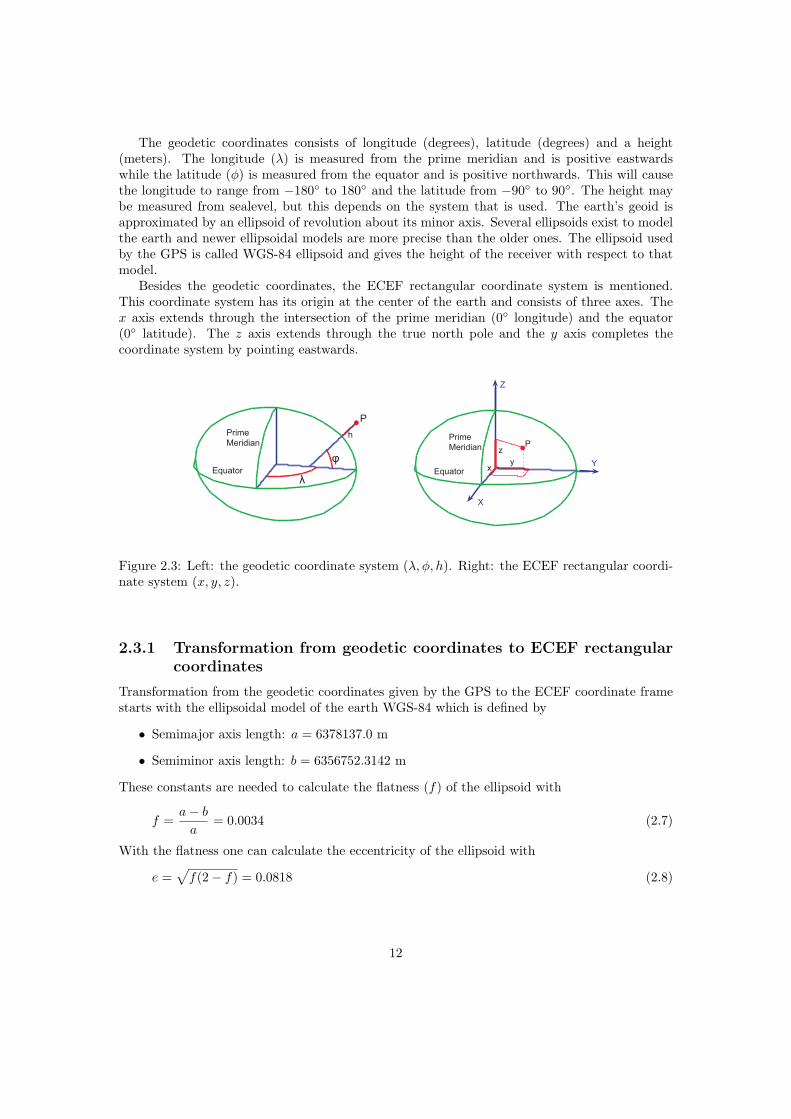
The geodetic coordinates consists of longitude (degrees), latitude (degrees) and a height(meters). The longitude (λ) is measured from the prime meridian and is positive eastwardswhile the latitude (φ) is measured from the equator and is positive northwards. This will causethe longitude to range from −180◦ to 180◦ and the latitude from −90◦ to 90◦. The height maybe measured from sealevel, but this depends on the system that is used. The earth’s geoid isapproximated by an ellipsoid of revolution about its minor axis. Several ellipsoids exist to modelthe earth and newer ellipsoidal models are more precise than the older ones. The ellipsoid usedby the GPS is called WGS-84 ellipsoid and gives the height of the receiver with respect to thatmodel.

Besides the geodetic coordinates, the ECEF rectangular coordinate system is mentioned.This coordinate system has its origin at the center of the earth and consists of three axes. Thex axis extends through the intersection of the prime meridian (0◦ longitude) and the equator(0◦ latitude). The z axis extends through the true north pole and the y axis completes thecoordinate system by pointing eastwards.

Figure 2.3: Left: the geodetic coordinate system (λ, φ, h). Right: the ECEF rectangular coordi-nate system (x, y, z).

2.3.1 Transformation from geodetic coordinates to ECEF rectangularcoordinates

Transformation from the geodetic coordinates given by the GPS to the ECEF coordinate framestarts with the ellipsoidal model of the earth WGS-84 which is defined by

• Semimajor axis length: a = 6378137.0 m

• Semiminor axis length: b = 6356752.3142 m

These constants are needed to calculate the flatness (f) of the ellipsoid with

f =a − b

a= 0.0034 (2.7)

With the flatness one can calculate the eccentricity of the ellipsoid with

e =√

f(2 − f) = 0.0818 (2.8)

12

The length of the normal to the ellipsoid, from the surface of the ellipsoid to its intersection withthe ECEF z axis, is

N(λ) =a

√

1 − e2 sin(λ)2(2.9)

Now the rectangular coordinates can be calculated as

x = (N + h) cos(λ) cos(φ) (2.10)

y = (N + h) cos(λ) sin(φ) (2.11)

z = (N(1 − e2) + h) sin(λ) (2.12)

2.3.2 Transformation from ECEF to tangent plane

In the previous section the transformation from the geodetic coordinates to ECEF rectangularcoordinates of an arbitrary point is given. These rectangular coordinates are still not very usefulat the mining site. Therefore these ECEF rectangular coordinates will be transformed to a localtangent reference frame. This transformation consists of a translation and two plane rotations.The first rotation is about the ECEF z axis to align the rotated y axis with tangent plane east:

R1 =

cos(φ) sin(φ) 0− sin(φ) cos(φ) 0

0 0 1

(2.13)

where φ is the longitude of the arbitrary point.A second rotation will be around the new y axis (y′) to align the new z axis with tangent

plane vertical down. This rotation is defined by

R2 =

− sin(λ) 0 cos(λ)0 1 0

− cos(λ) 0 − sin(λ)

(2.14)

Combining Eq. (2.13) and Eq. (2.14) results in an overall transformation defined by

Re2t = R2R1 =

− sin(λ) cos(φ) − sin(λ) sin(φ) cos(λ)− sin(φ) cos(φ) 0

− cos(λ) cos(φ) − cos(λ) sin(φ) − sin(λ)

(2.15)

After these rotations the coordinates must be translated to a more useful position at thesite. In this case the coordinates of the antenna of the base station (X0Y0Z0)’ will be used asthe origin of the local coordinate frame. So the local coordinates of the rover (X Y Z)′ can beobtained by subtracting the rotated position vector of the base station (X ′′

0 Y ′′

0 Z ′′

0 )′ from therotated position vector of the rover:

(X Y Z)′ = (x′′ y′′ z′′)′ − (X ′′

0 Y ′′

0 Z ′′

0 )′ (2.16)

ExampleThe antenna of the base station is located at geodetic coordinates

(λ, φ, h) = (−26.99649597◦, 152.82371005◦, 141.583 m)

13

of which the angles are in decimal degrees. Transformation from degrees into radians gives

(λ, φ, h) = (−0.4711777411 rad, 2.6672769155 rad, 141.583 m)

Calculation of the length of the normal to the ellipsoid from the surface of the ellipsoid to itsintersection with the ECEF z axis with Eq. (2.9) gives

N(λ) = 6.3825406528 · 106 m

With N(λ) the rectangular coordinates in the ECEF frame can be calculated with Eqs. (2.10)to (2.12) and result in

x0 = −5.0593609070 · 106 m

y0 = 2.5975122401 · 106 m

z0 = −2.8779378018 · 106 m

This point will be used as the origin of the local reference frame. The corresponding rotationmatrix has the following values:

RSH(e2t) =

−0.4038239476 0.2073261161 0.8910342872−0.4567298310 −0.8896054527 00.7926689604 −0.4069619394 0.4539360077

The coordinates of the rover will be rotated with the upper rotation matrix and afterwardstranslated with the rotated position vector of the base station.

2.4 Results

The first results from the GPS in autonomous mode are compared with the results of the GPS inRTK differential mode as shown in Figure (2.4). The coordinates are rotated and translated toa local reference frame with the base station at the origin. The left figure shows the uncorrectedGPS positions in time when the machine house swings. In this GPS mode the observations drifta couple meters resulting in a spiral in swing motion.In the right figure, the observations of the RTK corrected GPS are shown. In this GPS modethe observations do not drift resulting in a circle when the machine house swings.

One of the difficulties of differential GPS is finding the exact location of the base station.This has to be done with only one receiver which doesn’t give accurate results as mentionedearlier. Fortunately the base station is a stationary point and this makes it possible to averagethe observations over time (with the $PASHS,PPO,Y command). The effect of this command isshown in Figure (2.5). Without averaging the positions (plotted in black) drift meters resulting ina coarse path, while the averaged positions (plotted in grey) form a smooth path. The averagedpositions still drift meters within the first couple of hours, but after 23 hours the positions willdrift only within 10 cm (indicated with an arrow). When the receiver chooses another satellitefor its position calculation, the raw measurements may ’jump’ a couple meters. This is why theaveraged measurements (in grey) are almost two meters away from the raw measurements. Thiseffect can also be seen in the raw measurements (straight lines).

The position of the antenna at the site hut obtained by averaging the raw measurements ofthe GPS receiver over 23 hours is used as the base station position. However, this position maynot be the most accurate absolute position on the world but this will not affect the measuredposition of the rover relative to the base station. This is tested with the following experiment:the set position of the base station is changed to a position 1 meter north of its previous position

14

Figure 2.4: Left: uncorrected GPS observations during swing motion. Right: RTK correctedGPS observations during swing motion.

Figure 2.5: The effect of averaging the raw measurements of an autonomous GPS receiver.

to prove that the relative position of the rover is still correct. This means that the antenna ofthe base station is actually south and the observations of the rover should be moved one metersouthwards also.The results are shown in Figure (2.6). The grey circle represents the observations of the rover

15

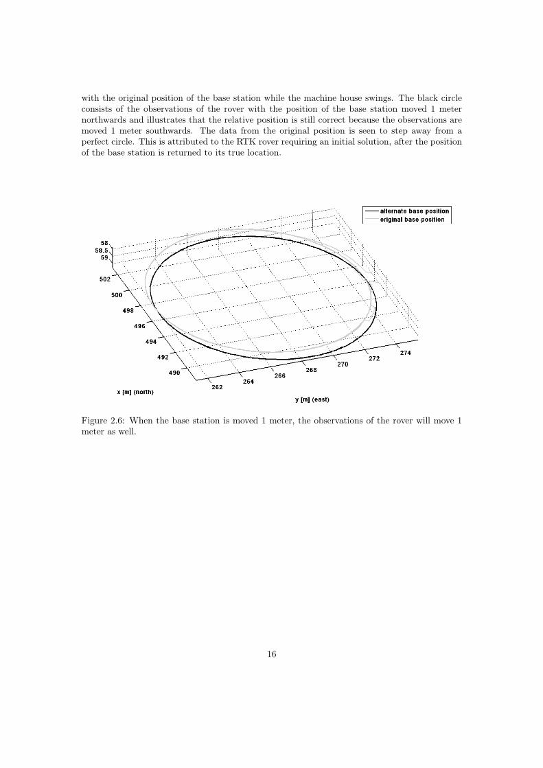
with the original position of the base station while the machine house swings. The black circleconsists of the observations of the rover with the position of the base station moved 1 meternorthwards and illustrates that the relative position is still correct because the observations aremoved 1 meter southwards. The data from the original position is seen to step away from aperfect circle. This is attributed to the RTK rover requiring an initial solution, after the positionof the base station is returned to its true location.

Figure 2.6: When the base station is moved 1 meter, the observations of the rover will move 1meter as well.

16

Chapter 3

IMU

3.1 Specifications and position

During stage two of the operating cycle of the shovel the pose estimator needs measurementsof the 3D pitch, roll, yaw and linear acceleration of the machine house at high frequencies. Inthis case a Crossbow DMU-VGX inertial measurement unit is used with a sample frequency upto 400 Hz. This IMU is able to measure three linear accelerations (x, y, z) and three angularvelocities with its gyros (θ1, θ2, θ3). The x axis of the IMU is in the same direction as the xaxis of the machine house. However, the z axis of the IMU extends downwards and results ina positive gravity measurement. Logically the y axis extends to the right side of the machinehouse completing the righthanded coordinate frame.

The IMU is placed inside the machine house of the EMS close to the swing axis in order toreduce centrifugal accelerations during swing motion (see Figure (3.1)). The position is 270 mmin negative x direction and 812 mm in negative y direction.

Figure 3.1: Crossbow DMU-VGX installed inside the machine house of the EMS.

17

3.2 Results

3.2.1 Gyros

The results of the IMU during the motions of the EMS are visualized in Figures (3.2) & (3.3).Figure (3.2) shows the measurements of the angular velocities around the x, y and z axes ofthe machine house during a step response test of the swing motion. The first step response isclockwise, the second response is anticlockwise. Both the tests use maximum torque and speedof the swing motor. The mean output and the standard deviation of the gyros during standstilland maximum swing speed are given in Table 3.1.

Table 3.1: Mean output and standard deviation of the gyros.

motion axis Mean [deg/s] Std. Dev. [deg/s]

Standstill θ1 1.602 0.035

θ2 -2.393 0.029

θ3 -0.723 0.033

max. clockwise θ1 1.619 0.035

θ2 -2.221 0.082

θ3 14.888 0.134

max. anticlockw. θ1 1.617 0.037

θ2 -2.411 0.053

θ3 -16.304 0.145

3.2.2 Accelerometers

Figure (3.3) illustrates the linear accelerations of the IMU in x, y and z directions. The acceler-ations in all three directions are due to gravity. The position of the shovel is not on flat groundbut on a slope. This will cause small accelerations in the x and y directions which change duringswing motion. The major part of the gravity is still in the z direction. More details about thiswill be given in Chapter 4. Besides the results of the gravity is the offset of the IMU itself andthe centrifugal accelerations. The mean output and the standard deviation of the accelerometersduring standstill are given in Table 3.2.

Table 3.2: Mean output and standard deviation of the accelerometers.

motion axis Mean [m/s2] Std. Dev. [m/s2]Standstill x -0.408 0.046

y 0.252 0.037z 9.818 0.028

18

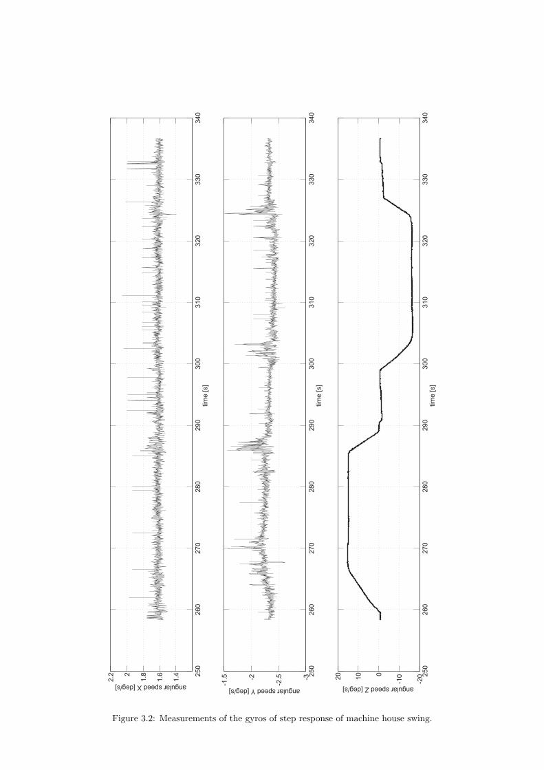
Figure 3.2: Measurements of the gyros of step response of machine house swing.

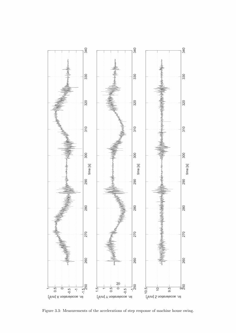
Figure 3.3: Measurements of the accelerations of step response of machine house swing.

20

3.2.3 Noise from crowd drive

In an EMS the motors for hoist, crowd and swing use a large amount of energy, therefore thearmature current of these motors reach high values up to hundreds of amperes. Because of thesehigh currents, the magnetic fields could cause noise on other instruments, especially measurementinstruments and associated power and data cabling, which therefore have to be shielded.In Figures (3.4) & (3.5) the measurements of the IMU are plotted against time while the crowddrive is commanded to execute step motions in alternate directions. The upper figure in bothFigures show the crowd motor speed. The three figures below show the measurements of thegyros and the accelerometers respectively. Especially the accelerations in x and z directions showsome activity while crowding. These are most likely the measured dynamics of the machine housebecause the crowd drive moves in the x–z plane and the vibration is not present in the othermeasurements of the IMU.

21

Figure 3.4: Noise from crowd drive on gyros.

Figure 3.5: Noise from crowd drive on accelerometers.

23

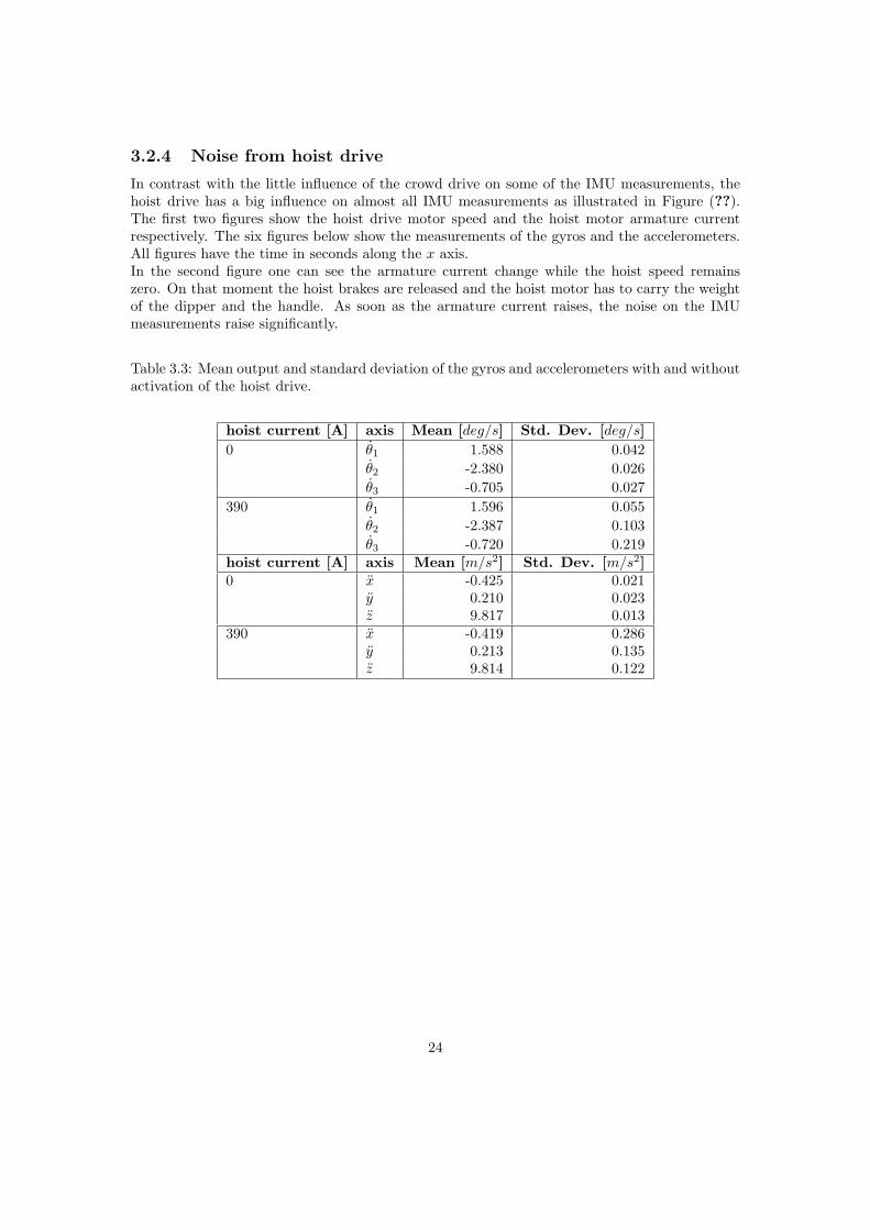
3.2.4 Noise from hoist drive

In contrast with the little influence of the crowd drive on some of the IMU measurements, thehoist drive has a big influence on almost all IMU measurements as illustrated in Figure (??).The first two figures show the hoist drive motor speed and the hoist motor armature currentrespectively. The six figures below show the measurements of the gyros and the accelerometers.All figures have the time in seconds along the x axis.In the second figure one can see the armature current change while the hoist speed remainszero. On that moment the hoist brakes are released and the hoist motor has to carry the weightof the dipper and the handle. As soon as the armature current raises, the noise on the IMUmeasurements raise significantly.

Table 3.3: Mean output and standard deviation of the gyros and accelerometers with and withoutactivation of the hoist drive.

hoist current [A] axis Mean [deg/s] Std. Dev. [deg/s]

0 θ1 1.588 0.042

θ2 -2.380 0.026

θ3 -0.705 0.027

390 θ1 1.596 0.055

θ2 -2.387 0.103

θ3 -0.720 0.219hoist current [A] axis Mean [m/s2] Std. Dev. [m/s2]0 x -0.425 0.021

y 0.210 0.023z 9.817 0.013

390 x -0.419 0.286y 0.213 0.135z 9.814 0.122

24

Figure 3.6: Noise from hoist drive on gyros.

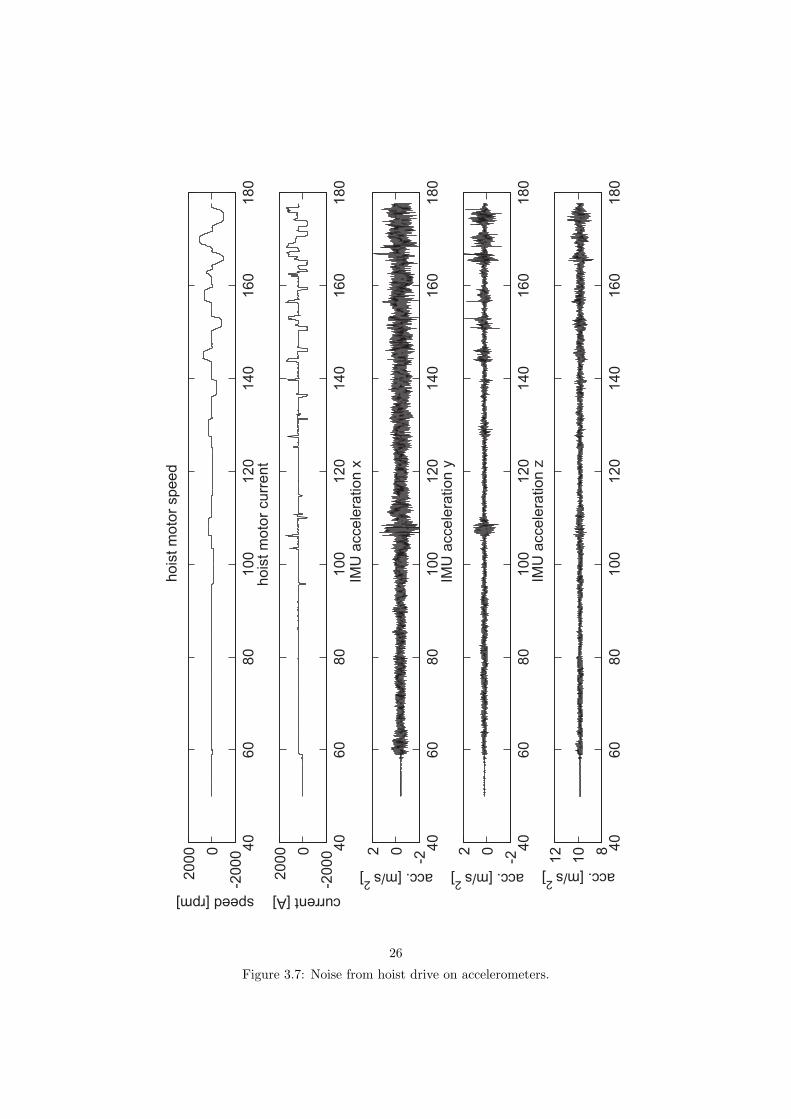
Figure 3.7: Noise from hoist drive on accelerometers.

26

Chapter 4

Inclinometer

4.1 Specifications and position

With the IMU and GPS installed in the EMS the location in a local reference frame and themotions can be measured and calculated. However, absolute pitch and roll of the EMS is onlyknown via integration of IMU rate gyro measurements. The results of the accelerometers inthe IMU showed that gravity caused accelerations in x and y directions as the shovel swings.This means that the shovel is on an angle. The IMU may be used to calculate the angle, butwith smaller angles this is not a precise instrument. One may use the observations of the GPSduring swing motion in order to calculate this angle but this will take a lot of time. Thereforean inclinometer is installed next to the IMU to provide an absolute inclination reference, close tothe swing axis of the machine house. This position will have less influence of centrifugal effects.

In Figure (4.1) one can see the position of the inclinometer (cylinder indicated with thearrow) on the platform next to the IMU. It is a Jewell Instruments LCF 196 which is a dual axisinclinometer. The input range is ±14.5◦ in x & y and the output range is ±5.0 Volts.

4.2 Results

Figure (4.2) shows the output of the x & y axes of the inclinometer during a continuous an-ticlockwise swing motion. Also in this test the shovel is positioned on an angle causing theoutput to be sinusoids. The mean of the sinusoids should be zero and the maxima representthe angle of the shovel on the ground. However, the horizontal lines, which are the means over9 periods for the x & y axes, have values of 0.22 and 0.15 Volts for x & y respectively. Theyrepresent the offset of the two axes of the inclinometer from the house frame. The offset ofthe inclinometer itself is 0.0018 V and 0.0107 V so the instrument is mounted on an angle of(0.22 − 0.0018)(14.5/5.0) = 0.633◦ in x and (0.15 − 0.0107)(14.5/5.0) = 0.404◦ in y.

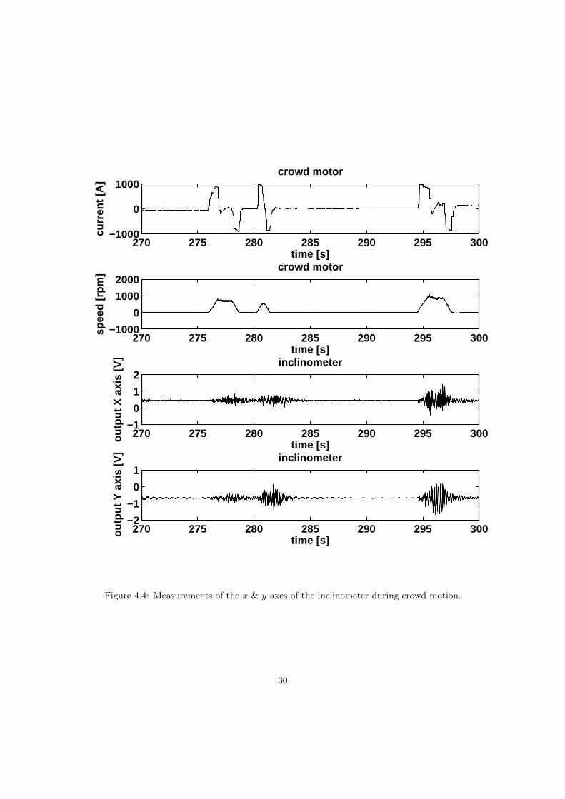
Unfortunately the conditions on an EMS are not always very good for measurements. Duringall motions (hoisting, crowding, swinging and propelling) the whole machine house is shakingand high currents of the motors may cause noise on the signals.

One of the sources of noise is the hoist drive. While the EMS is at standstill, the hoist driveis turned on resulting in the noise on the inclinometer output indicated in Figure (4.3). Thisnoise looks most on the dynamics of the inclinometer because the noise has its highest valueswhen the hoist drive is actually working. Also the crowd drive influences the results illustratedin Figure (4.4).

27

Figure 4.1: Drawing (left) and photo (right) of the platform on which the inclinometer and theIMU are mounted

100 150 200 250 300 350−1

−0.5

0

0.5

1

1.5

time [s]

outp

ut x

axi

s [V

]

100 150 200 250 300 350−1

−0.5

0

0.5

1

1.5

time [s]

outp

ut y

axi

s [V

]

Figure 4.2: Measurements of the x & y axes of the inclinometer during swing motion.

28

40 45 50 55 60 65 70 75 80−1000

0

1000

2000hoist motor

time [s]

curr

ent [

A]

40 45 50 55 60 65 70 75 80−200

0

200

400

time [s]

spee

d [r

pm]

hoist motor

40 45 50 55 60 65 70 75 800

0.5

1

1.5

time [s]

outp

ut x

axi

s [V

]

inclinometer

40 45 50 55 60 65 70 75 80−1

−0.5

0

time [s]

outp

ut y

axi

s [V

]

inclinometer

Figure 4.3: Measurements of the x & y axes of the inclinometer during hoist motion.

29

270 275 280 285 290 295 300−1000

0

1000crowd motor

time [s]

curr

ent [

A]

270 275 280 285 290 295 300−1000

0

1000

2000

time [s]

spee

d [r

pm]

crowd motor

270 275 280 285 290 295 300−1

0

1

2

time [s]

outp

ut X

axi

s [V

] inclinometer

270 275 280 285 290 295 300−2

−1

0

1

time [s]

outp

ut Y

axi

s [V

] inclinometer

Figure 4.4: Measurements of the x & y axes of the inclinometer during crowd motion.

30

Chapter 5

Tachometers

5.1 Installation of Tachometers

In order to calculate the speed of the three motion axes, the motor speeds are measured. Fromthe machine signals one may use the voltages and currents to obtain the motor speeds, but thosesignals are heavily influenced by motor test parameters set manually during machine commis-sioning. Tachometers (tachogenerators) are installed on the hoist, crowd and swing motors toverify the motor speeds obtained from the Centurion supervisory controller. Figure (5.1) showsa tachometer installed on the hoist drive indicated with a black arrow. Part of the hoist drumcan be seen at the right of the figure. All tachometers are identical and give 7 Volts per 1000rpm.The test results of each tachometer are shown in the next figures and are compared with themotor speeds obtained obtained from Centurion.

Figure 5.1: Tachometer installed on the hoist motor.

31

5.2 Measurements of tachometers

5.2.1 Swing motor

The motor speed obtained with the machine signals (profibus) is 98% of the speed measuredwith the tachometer illustrated in Figure (5.2). Noise on other tachometers while swinging isshown in Figure (5.3).

Figure 5.2: Measurements of the swing tacho during a step response test.

Figure 5.3: Noise on other tachometers during swing step response test.

32

5.2.2 Crowd motor

The crowd motor speed obtained with the machine signals (profibus) is 125% of the speed mea-sured with the tachometer. This is a significant difference and suggests an erroneous parameterin the Centurion crowd motor speed parameters. Noise on other tachometers while swinging isshown in Figure (5.5).

Figure 5.4: Measurements of the crowd tacho during a step response test.

Figure 5.5: Noise on other tachometers during crowd step response test.

33

5.2.3 Hoist motor

The hoist motor speed obtained with the machine signals (profibus) is 104% of the speed mea-sured with the tachometer. Noise on other tachometers while swinging is shown in Figure (5.7).

Figure 5.6: Measurements of the hoist tacho during a step response test.

Figure 5.7: Noise on other tachometers during hoist step response test.

34

Chapter 6

Conclusion

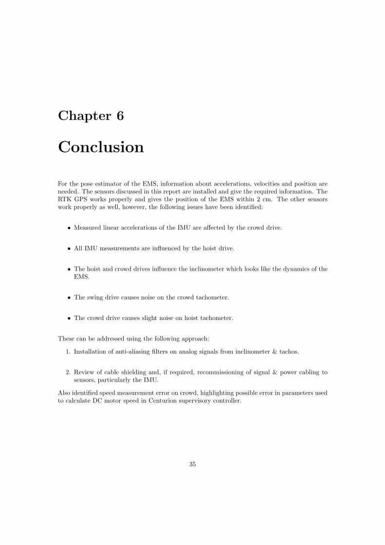
For the pose estimator of the EMS, information about accelerations, velocities and position areneeded. The sensors discussed in this report are installed and give the required information. TheRTK GPS works properly and gives the position of the EMS within 2 cm. The other sensorswork properly as well, however, the following issues have been identified:

• Measured linear accelerations of the IMU are affected by the crowd drive.

• All IMU measurements are influenced by the hoist drive.

• The hoist and crowd drives influence the inclinometer which looks like the dynamics of theEMS.

• The swing drive causes noise on the crowd tachometer.

• The crowd drive causes slight noise on hoist tachometer.

These can be addressed using the following approach:

1. Installation of anti-aliasing filters on analog signals from inclinometer & tachos.

2. Review of cable shielding and, if required, recommissioning of signal & power cabling tosensors, particularly the IMU.

Also identified speed measurement error on crowd, highlighting possible error in parameters usedto calculate DC motor speed in Centurion supervisory controller.

35

Appendix A

List of abbreviations

A.1 List of Abbreviations

C/A Coarse AcquisitionCBN Message containing the position.CPD Carrier Phase Differential (used as synonym of RTK)ECEF Earth Centered, Earth FixedEMS Electric Mining ShovelGPS Global Positioning SystemIMU Inertial Measurement UnitNMEA Output messages of position.P(Y) Y encrypted Precision code.RTCM Radio Technical Commission for Maritime ServicesRTK Real Time KinematicSA Selective AvailabilityUTC Coordinated Universal Time (current time at Greenwich)

36

Appendix B

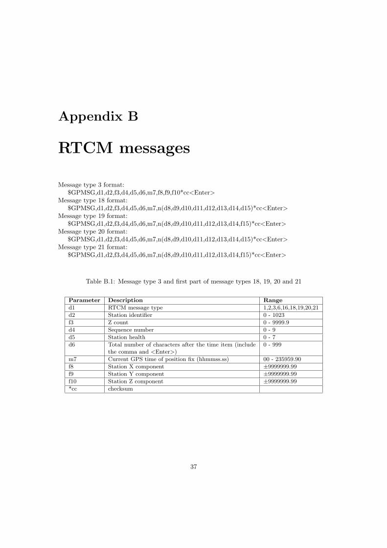
RTCM messages

Message type 3 format:$GPMSG,d1,d2,f3,d4,d5,d6,m7,f8,f9,f10*cc<Enter>

Message type 18 format:$GPMSG,d1,d2,f3,d4,d5,d6,m7,n(d8,d9,d10,d11,d12,d13,d14,d15)*cc<Enter>

Message type 19 format:$GPMSG,d1,d2,f3,d4,d5,d6,m7,n(d8,d9,d10,d11,d12,d13,d14,f15)*cc<Enter>

Message type 20 format:$GPMSG,d1,d2,f3,d4,d5,d6,m7,n(d8,d9,d10,d11,d12,d13,d14,d15)*cc<Enter>

Message type 21 format:$GPMSG,d1,d2,f3,d4,d5,d6,m7,n(d8,d9,d10,d11,d12,d13,d14,f15)*cc<Enter>

Table B.1: Message type 3 and first part of message types 18, 19, 20 and 21

Parameter Description Range

d1 RTCM message type 1,2,3,6,16,18,19,20,21

d2 Station identifier 0 - 1023

f3 Z count 0 - 9999.9

d4 Sequence number 0 - 9

d5 Station health 0 - 7

d6 Total number of characters after the time item (includethe comma and <Enter>)

0 - 999

m7 Current GPS time of position fix (hhmmss.ss) 00 - 235959.90

f8 Station X component ±9999999.99

f9 Station Y component ±9999999.99

f10 Station Z component ±9999999.99

*cc checksum

37

Table B.2: Remaining for message type 18 and 20.

Parameter Description Range

d8 L1 or L2 frequency 00...01

d9 GPS time of measurement 0..599999 [usec]

d10 half/full L2 wavelength indicator 0 - full, 1 - half

d11 CA code /P code indicator 0 - CA, 1 -P

d12 SV prn 1..32

d13 data quality 0..7

d14 cumulative loss of continuity indi-cator

0..31

d15 type 18 - carrier phase ±8388608 full cycles with resolution of1/256 full cycle±16777216 half cycles with resolution of1/128 half cycle

type 20 - carrier phase correction ±32768 full wavelengths with resolution1/256 full wavelength±65536 half wavelengths with resolution of1/128 half wavelength

Table B.3: Remaining for message type 19 and 21.

Parameter Description Range

d8 L1 or L2 frequency 00...01

d9 Smoothing interval 00 - 0..1 min01 - 1..5 min10 - 5..15 min11 - indefinite

d10 GPS time of measurement 0..599999 [usec]

d11 CA code /P code indicator 0 - CA, 1 -P

d12 SV prn 1..32

d13 data quality 0..7

d14 multipath error 0..15

f15 type 19 - pseudorange 0..85899345.90 meterstype 21 - pseudorange ±655.34[0.02 meter] when pseudorange

scale factor is 0±10485.44 [0.32 meter] when pseudorangescale factor is 1 (default)

38

Appendix C

NMEA messages

Format of NMEA POS message and GGA message:$PASHR,POS,d1,d2,m3,m4,c5,m6,c7,f8,f9,f10,f11,f12,f13,f14,f15,f16,s17*cc<Enter>$GPGGA,m1,m2,c3,m4,c5,d6,d7,f8,f9,M,f10,M,f11,d12*cc<Enter>

Table C.1: Contents of NMEA position response messages (POS) from the rover.

Parameter Description Range

d1 Raw/differential position 0 - 30:Raw; position is not differentially corrected1:Position is differentially corrected with RTCM code2:Position is differentially corrected with CPD float solu-tion3:Position is CPD fixed solution

d2 Number of SVs used in position fix 3 - 12

m3 Current UTC time of position fix (hhmmss.ss) 00 - 235959.90

m4 Latitude component of position in degrees and decimalminutes (ddmm.mmmmmm)

0 - 90

c5 Latitude sector, N = North, S = South N/S

m6 Longitude component of position in degrees and decimalminutes (dddmm.mmmmmm)

0 - 180

c7 Longitude sector E = East, W = West W/E

f8 Altitude above whatever datum has been selected in me-ters. For 2-D position computation this item containsthe altitude held fixed.

-1000.000 - 18000.000

f9 reserved

f10 True track/course over ground in degrees 0 - 359.9

f11 Speed over ground in knots 0 - 999.9

f12 Vertical velocity in decimeters per second ±999.9

f13 PDOP - position dilution of precision 0 - 99.9

f14 HDOP - horizontal dilution of precision 0 - 99.9

f15 VDOP - vertical dilution of precision 0 - 99.9

f16 TDOP - time dilution of precision 0 - 99.9

s17 Firmware version ID 4 char string

*cc checksum

39

Table C.2: Contents of NMEA position response messages (GGA) from the rover.

Parameter Description Range

m1 Current UTC time of position fix (hhmmss.ss) 00 - 235959.90

m2 Latitude component of position in degrees and decimalminutes (ddmm.mmmmmm)

0 - 90

c3 Latitude sector, N = North, S = South N/S

m4 Longitude component of position in degrees and decimalminutes (dddmm.mmmmmm)

0 - 180

c5 Longitude sector E = East, W = West W/E

d6 Raw/differential position 0 - 30:Raw; position is not differentially corrected1:Position is differentially corrected with RTCM code2:Position is differentially corrected with CPD float solu-tion3:Position is CPD fixed solution

d7 Number of SVs used in position fix 3 - 12

f8 HDOP - horizontal dilution of precision 0 - 99.9

f9 Geoidal Height (Altitude above mean sea level). -1000.000 - 18000.000

M Altitude units M = meters ’M’

f10 Geoidal separation in meters ± 999.999

M Geoidal separation units M = meters ’M’

f11 Age of differential corrections (seconds) 0-999 (RTCM mode) 0-99 (CPD)

d12 Base station ID (RTCM only) 0 - 1023

*cc checksum

40

Bibliography

[1] Jay A. Farrell & Matthew Barth: The Global Positioning System & Inertial Navigation,McGraw-Hill, California, 1999

[2] Z-Extreme Technical Reference Manual - Ashtech Precision Products, Magellan Corpora-tion.

[3] Janet Brown Neumann, Keith J. VanDierendock, Allan Manz, and Thomas J. Ford: Real-Time Carrier Phase Positioning Using the RTCM Standard Message Types 20/21 and 18/19.- NovAtel Inc.

[4] Dennis G. Milbert, Ph.D. and Dru A. Smith, Ph,D.: Converting GPS Height into NAVD88Elevation with the GEOID96 Geoid Height Model - National Geodatic Survey, NOAA.

41