Darmstadt Discussion Papers

in Economics

Investors Facing Risk II:

Loss Aversion and Wealth Allocation When

Utility Is Derived From Consumption and

Narrowly Framed Financial Investments

Erick W. Rengifo, Emanuela Trifan

Nr. 181

Arbeitspapiere

des Instituts fur Volkswirtschaftslehre

Technischen Universitat Darmstadt

Investors Facing Risk II

Loss Aversion and Wealth Allocation When Utility Is

Derived From Consumption and Narrowly Framed

Financial Investments∗

Erick W. Rengifo† Emanuela Trifan‡

February 2007

Abstract

This paper studies the attitude of non-professional investors towards financiallosses and their decisions concerning wealth allocation among consumption, risky,and risk-free financial assets. We employ a two-dimensional utility setting in whichboth consumption and financial wealth fluctuations generate utility. The perceptionof financial wealth is modelled in an extended prospect-theory framework that ac-counts for both the distinction between gains and losses with respect to a subjectivereference point and the impact of past performance on the current perception ofthe risky portfolio value. The decision problem is addressed in two distinct equilib-rium settings in the aggregate market with a representative investor, namely withexpected and non-expected utility. Empirical estimations performed on the basis ofreal market data and for various parameter configurations show that both settingssimilarly describe the attitude towards financial losses. Yet, the recommendationsregarding wealth allocation are different. Maximizing expected utility results onaverage in low total-wealth percentages dedicated to consumption, but supportsmyopic loss aversion. Non-expected utility yields more reasonable assignments toconsumption but also a high preference for risky assets. In this latter setting, my-opic loss aversion holds solely when financial wealth fluctuations are viewed as themain utility source and in very soft form.

Keywords : prospect theory, Value-at-Risk, loss aversion, expected utility, non-expected

utility

JEL Classification: C32, C35, G10

∗The authors would like to thank Horst Entorf for helpful suggestions. The usual disclaimers apply.†Fordham University, New York, Department of Economics. 441 East Fordham Road, Dealy Hall,

Office E513, Bronx, NY 10458, USA, phone: +1(718) 817 4061, fax: +1(718) 817 3518, e-mail: rengi-fomina@fordham.edu

‡Darmstadt University of Technology, Institute of Economics, Department of Applied Economics andEconometrics, 15 Marktplatz, 64283 Darmstadt, Germany, phone: +49(0) 6151 162636, fax: +49 (0)6151165652, e-mail: trifan@vwl.tu-darmstadt.de

2

1 Introduction

Optimal allocation of resources among different activities that generate utility represents

a main decision problem in everyday life. For each individuum, the first and most im-

portant source of individual utility is consumption. Additionally, people who are active

in financial markets derive utility from their investments. This paper addresses the atti-

tude towards financial losses of individual (non-professional) investors who narrowly frame

risky investments and change current perceptions subject to the past performance of these

investments. Equally, we analyze how (non-professional) investors split their money be-

tween consumption and (risky and risk-free) financial projects as a consequence of their

loss attitude.

Our work is based on the theoretical framework introduced in Barberis, Huang, and

Santos (2001) and developed in Barberis, Huang, et al. (2003, 2004). Several ideas

developed in these papers have already been incorporated by Rengifo and Trifan (2006)

into the portfolio optimization setting developed in Campbell, Huisman, and Koedijk

(2001). In particular, Rengifo and Trifan (2006) describe how individual perceptions of

risky financial investments impact on the optimal composition of a risky portfolio and the

money to be invested in risk-free assets. Their focus lies thus on capital allocation decisions

of non-professional investors, where finding the optimal mix of risky assets is assumed

to represent the task of professional portfolio managers. Meanwhile, non-professional

investors are left with the choice between the risky portfolio as a whole and a risk-free

asset. In this context, individual utility is considered to exclusively originate in financial

wealth fluctuations. Thus, the designed utility setting in Rengifo and Trifan (2006) can

be regarded as one-sided.

The present paper aims at enlarging this perspective to what we denote as two-

dimensional utility. Specifically, our setting accounts for consumption as additional source

of utility besides the utility derived from financial investments. Our non-professional in-

vestors have now to decide upon the optimal wealth allocation between consumption and

financial investments in general, where the latter category offers a further choice between

the risky portfolio and a risk-free asset. We adopt the formal views in Rengifo and Tri-

fan (2006) regarding the subjectively perceived value of risky investments (denoted as the

prospective value) and how it enters the decision problem of non-professional investors. In

addition, we rely on two theoretical approaches proposed in Barberis and Huang (2004a,b),

according to which investors decisions rely on the maximization of either expected utility

or of recursive non-expected utility with first-order risk aversion. In both cases, the utility

function is shaped in order to account for the narrow framing of financial investments and

for the influence of past portfolio performance on current perceptions of risky investments.

Moreover, for a better description of the individual attitude towards financial losses, two

3

further measures used in Rengifo and Trifan (2006) are adopted, namely the loss aversion

index (LAi) and the global first-order risk aversion (gRA).

In order to analyze the loss attitude and the wealth allocation in this context, we

proceed in line with Barberis and Huang (2004a,b). Thus, we first derive necessary and

sufficient equilibrium conditions on the aggregate market with a representative investor.

Second, fixing general market parameters (such as the dynamics of consumption and

of expected returns), these conditions serve to derive the equilibrium expressions of the

variables of interest. These variables are either common to both considered approaches

with expected and non-expected utility (such as the prospective value, the loss aver-

sion coefficient, and further measures of the attitude towards losses) or specific (such as

the time-discounting factor of the utility function in the expected-utility setting, or the

percentages of total wealth dedicated to consumption and of post-consumption wealth

invested in risky assets in the non-expected utility setting).

In the sequel, the theoretical part developed so far is empirically implemented and

amended. To this end, we rely on the same data set as in Rengifo and Trifan (2006),

consisting of the SP500 and the 10-year bond nominal returns, as proxies for a well

diversified risky portfolio and the risk-free investment, respectively. In addition, we employ

aggregate per-capita consumption data that allow us to analyze the investor loss attitude

and the decisions concerning the wealth allocation for two different evaluation frequencies

of the risky-portfolio performance (of one year and three months). We simulate how non-

professional investors who follow the logic of our model make decisions in an environment

where consumption and financial markets are characterized by general parameters derived

from the sets of real data at hand. In so doing, we consider various configurations of

the individual (behavioral) parameters (such as the consumption-based risk aversion, the

narrow-framing degree, the penalties imposed on past financial losses, and the initial

coefficient of loss aversion). Moreover, we attempt to avoid the impossibility of covering

current consumption needs from financial revenues over the entire investing interval, by

considering that investors periodically dispose of exogenous additional incomes. In order

to investigate the sensitivity of our model to this assumption, we further consider different

levels of the additional income that are further shaped to render comparable the two

approaches with expected and non-expected utility.

In both considered utility settings, we estimate the prospective values ascribed to

risky investments and derive the corresponding loss aversion coefficients in equilibrium.

These estimates also serve to compute the equilibrium values of the extended measures

of individual attitude to financial risk, namely the loss aversion index and the global

first-order risk aversion. In addition, the discounting factor of the utility function is

additionally estimated from the equilibrium conditions in the expected-utility setting.

4

Here, the wealth percentages dedicated to consumption, risky, and riskless assets can

be assessed on average only. By contrast, the non-expected utility approach delivers

direct estimates of the proportions of total wealth allocated to consumption and of post-

consumption wealth invested in risky assets.

The empirical findings can be summarized as follows. On the one hand, maximizing

expected or non-expected utility derived from consumption and narrowly framed finan-

cial investments, generates similar attitudes towards financial losses. In particular, the

loss aversion coefficient in equilibrium lies close to the “neutral” value of 1, which shows

that investors who derive utility from twofold source are more relaxed towards financial

losses than suggested by the original prospect theory (that proposes the value of 2.25 for

the same coefficient). Moreover, the same coefficient increases for either higher degrees

of narrow framing, or when no penalties are imposed on past losses, other things being

equal. Mostly, it also decreases c.p. as the risky performance is more frequently evaluated,

but the direction of this variation is more sensitive with respect to the magnitude of the

additional income in the non-expected utility setting. In addition, the loss aversion index

in equilibrium follows closely in value and the evolution pattern of the simple loss aversion

coefficient. The global first-order risk aversion exhibits similar development and appears

to more consistently describe the actual investor attitude towards financial losses. More-

over, both approaches entail negative estimates of the prospective value in equilibrium,

suggesting that financial investments decrease the overall utility. A final common finding

refers to the fact that both an excessive consumption-related risk aversion and the lack of

narrow framing of financial investments entail implausible equilibrium-estimates.

On the other hand, the two approaches provide different recommendations regarding

the wealth allocation between consumption and (risky and riskless) financial assets. Note

that in both settings, this allocation substantially varies with the magnitude of the ad-

ditional income. Investors who maximize expected utility appear to be on average very

open to financial investments, as they consume only small fractions of their total wealth

(less than one-fifth). The myopic loss aversion holds in this setting, as the total-wealth

percentages invested in risky assets diminish to almost one-third when the risky perfor-

mance is evaluated every three-months instead of once a year. By contrast, reaching the

aggregate equilibrium with non-expected utility requires more reasonable wealth percent-

ages dedicated to consumption (namely over one-third). In exchange, investors are now

very open to risky investments and even borrow money to increase the value of their

risky portfolios. The resulting parts of total wealth that flow into risky investments are

substantially higher but also more variable subject to the magnitude of the additional

income, relative to the expected-utility setting. Finally, myopic loss aversion holds under

the maximization of non-expected utility only when investors regard narrowly framed fi-

5

nancial investments as a more important source of utility relative to consumption. Even

in such situations the sums allocated to risky assets are only minimally reduced as their

performance is revised more often.

The remainder of the paper is organized as follows. The theoretical framework is

presented in Section 2. In this context, Section 2.1 provides a brief review of the general

purpose of the model in Rengifo and Trifan (2006) and refreshes the definitions of variables

of interest for the present paper. The extension of this model to the two-dimensional utility

setting is undertaken in Section 2.2, which details the approaches with expected and non-

expected utility. Section 3 presents the empirical implementation of our theoretical model

for the expected-utility framework in Section 3.2, and the non-expected utility setting in

Section 3.3. The main findings under these two theoretical approaches are confronted in

the subsequent Section 3.4. Finally, Section 4 summarizes our findings. Further numerical

results are included in the Appendix.

2 Theoretical model

This section presents the theoretical framework describing how non-professional investors

perceive financial risks and accordingly allocate their wealth between consumption and

financial investments in order to maximize perceived utility. In line with Barberis and

Huang (2004a,b), we adopt two distinct formulations of the maximization problem, first

around expected utility and, second, around recursive non-expected utility with first-order

risk aversion. Both settings account for narrow framing of financial projects and for the

influence of past performance on the perceived prospective value of risky investments.

2.1 A one-dimensional utility framework

One of the most important decisions in everyday life is how to allocate money among

different type of activities. These activities may be either necessary and/or can generate

further revenues. In the latter category, investing in financial assets has nowadays become

one of the most popular alternatives. This widespread trend of ordinary people turning

into “investors” is due at least in part to the formidable accessibility of information con-

cerning financial markets, at almost no cost and in almost no time. Under the pressure of

the huge amount and intensity of such information, even non-professional investors may

have no choice but to become overly concerned with their financial investments. This

phenomenon of putting excessive emphasis on financial investments is denoted in tech-

nical terms as “narrow framing”. Under narrow framing, allocating the “right” amount

of money first to financial investments in general, then across different financial assets,

turns into a central decision. Also, financial investments are perceived as distinct and

6

overly important generators of individual utility. This dissociates the decisions upon

wealth allocation from the naturally larger context with multiple utility generators (such

as consumption or other factors that do not exclusively apply to financial markets).

Drawing on this idea, Rengifo and Trifan (2006) model the attitude towards financial

risks and the decision making of non-professional investors regarding the optimal wealth

allocation among different financial assets. In so doing, they assume that investors derive

utility merely from financial investments. Their theoretical analysis develops in the port-

folio optimization framework suggested in Campbell, Huisman, and Koedijk (2001), where

market risk is measured by the Value-at-Risk (VaR) and enters the optimization problem

in form of a specific constraint. In particular, individual non-professional investors fix in

a first step their desired VaR-levels (denoted VaR*) according to their subjective prefer-

ences and perceptions. The choice of VaR* takes place outside of the risky portfolio so

to speak, in the sense that it precedes and hence it is not influenced by its composition.

The individually chosen VaR* is then communicated to professional portfolio managers.

They are in charge of the optimal money allocation among risky assets, in other words

of decisions inside of the risky portfolio. In a second step, considering the given VaR*,

portfolio managers determine the optimal composition of the risky portfolio and implicitly

the sum to be invested in risk-free assets. In so doing, professional managers help their

non-professional clients to solve the problem of optimally allocating money between risky

and risk-free assets.

The present work builds on the model in Rengifo and Trifan (2006) and extends it

for the case when investors derive utility not only from financial investments, but also

from consumption. Before entering into the details of this extended framework, we briefly

review the main model structure and the notions defined and applied in Rengifo and

Trifan (2006).

In order to quantify the formation of the desired VaR*-level in investor minds, Rengifo

and Trifan (2006) adopt the extended prospect theory framework developed in Bar-

beris, Huang, and Santos (2001). This framework models individual perceptions of risky

projects. Accordingly, the subjective perception of one unit of risky investment is cap-

tured by an extended value function vt+1. As in the original prospect theory of Kahneman

and Tversky (1979, 1992), this value function accounts for the distinct perception of gains

and losses with respect to a subjective reference point and the higher reluctance to losses.

In addition, it is designed to capture the possible influence of past performance on the

current risk perception. We apply the definitions of the value function proposed in Section

7

2.2 of Rengifo and Trifan (2006), namely:

vt+1 =

St(Rt+1 − Rft) , for Rt+1 ≥ Rft

λSt(Rt+1 − Rft) + (λ − 1)(St − Zt)Rft , for Rt+1 < Rft

, for zt ≤ 1 (1)

and

vt+1 =

St(Rt+1 − Rft) , for Rt+1 ≥ Rft

λSt(Rt+1 − Rft) + k(Zt − St)(Rt+1 − Rft) , for Rt+1 < Rft

, for zt > 1, (2)

where k > 0 represents the sensitivity to past losses and λ > 0 the individual loss aversion

coefficient (with λ ≥ 1 indicating loss aversion in strict sense). Moreover, Rt+1 stands

for the next-period portfolio returns and Rft for the risk-free returns. Finally, St denotes

the current value of the risky investment, while Zt is a benchmark level for past portfolio

performance, so that St−Zt accounts for the so-called cushion of past gains and/or losses

generated by the risky portfolio.

Denoting the equity premium by xt+1 = Rt+1−Rft and the probability of experiencing

past gains by πt = P (Zt ≤ St), Equations (1) and (2) can be pooled to a single expression

that accounts for both cases with prior gains (zt ≤ 1) and prior losses (zt > 1), namely:

vt+1 =

Stxt+1 , for xt+1 ≥ 0

[λSt − (1 − πt)k(St − Zt)]xt+1 + πt(λ − 1)Rft(St − Zt) , for xt+1 < 0,

On the basis of the perception of financial investments captured in the value functions

from Equations (1) and (2), Rengifo and Trifan (2006) define the maximum risk level

desired (accepted) by individual (non-professional) investors VaR* as:

VaR∗

t+1 = λStEt[xt+1]

+ [(πt − ϕ√

πt(1 − πt))(λ − 1)Rft − (1 − πt + ϕ√

πt(1 − πt))kEt[xt+1]](St − Zt),

(3)

where Et[xt+1] = Et[Rt+1] − Rft represents the expected equity premium.

As mentioned above, once this VaR* has formed in investor minds it is communicated

to the portfolio manager in the form of a fixed (so to speak “portfolio-exogenous”) risk

level. It hence flows into the problem of optimization inside the risky portfolio as risk

constraint. According to Campbell, Huisman, and Koedijk (2001), finding the optimal

capital allocation implies the derivation of the optimal investment in risk-free assets. This

8

is referred as the optimal amount of money to be borrowed or lent and yields:

Bt =VaR∗ + VaR

Rft − qt(w∗

t , α), (4)

where Bt > 0 (Bt < 0) stands for borrowing (lending), VaR=Wt[qt(w∗

t , α) − 1] represents

the so-called portfolio Value-at-Risk, w∗

t the optimal portfolio weights, and qt(wt, α) the

quantile of the distribution of portfolio returns at a given confidence level α.

Central to the analysis conducted in Rengifo and Trifan (2006), on which the present

work is based, is the derivation of the so-called prospective value Vt+1. This variable

captures the subjectively perceived utility of the risky portfolio, which non-professional

investors aim at maximizing.1 According to Equation (2.23) in Rengifo and Trifan (2006),

the prospective value can be formally defined as:

Vt+1 = [ωt +(1−ωt)λ]StEt[xt+1]+ (1−ωt)[πt(λ−1)Rft − (1−πt)kEt[xt+1]](St −Zt), (5)

where ωt = P (Et[Rt+1] ≥ Rft) is the probability of having a positive expected equity

premium Et[xt+1] ≥ 0. Moreover, Rengifo and Trifan (2006) distinguish in Equation

(5) between the PT-effect and the cushion effect. The former refers to the first term

on the right-hand side and stems from the value function formulation in the original

prospect theory. The latter effect denotes the second term on the right-hand side of

Equation (5) and has as its source the prior gains and losses accumulated from trading

the risky portfolio. The present work aims at determining the prospective value ascribed

by the representative investor who derives utility from both consumption and financial

investments in the market equilibrium.

From the prospective value in equilibrium, we subsequently determine the equivalent

coefficient of loss aversion λt+1. Formally, this yields:

λt+1 =Vt+1 − ωtStEt[xt+1] + (1 − ωt){πtRft + (1 − πt)kEt[xt+1]}(St − Zt)

(1 − ωt){StEt[xt+1] + πtRft(St − Zt)}. (6)

This coefficient plays a central role in our model, as it represents a measure of the attitude

towards financial losses and previous research suggests concrete values for it (such as 2.25

in the prospect theory).

As Rengifo and Trifan (2006) note, the joint impact of the loss aversion coefficient λ

and of past negative performance k changes the actual investor aversion to financial losses.

1Note that the term “maximization” shall be understood here in a general, lax sense (rather as“optimization”). In essence, the non-professional investors in Rengifo and Trifan (2006) are consideredrather unsophisticated, and hence do not have to tackle any maximization problem in strict mathematicalsense. Yet, these investors (as every person) attempt to perform most useful actions, given real constraints(such as their individual loss aversion, the past performance of their risky portfolios, etc.). Recall alsothat utility is assumed to exclusively emanate from investment decisions.

9

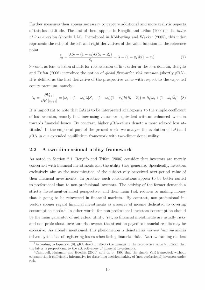
Further measures then appear necessary to capture additional and more realistic aspects

of this loss attitude. The first of them applied in Rengifo and Trifan (2006) is the index

of loss aversion (shortly LAi). Introduced in Kobberling and Wakker (2005), this index

represents the ratio of the left and right derivatives of the value function at the reference

point:

λt =λSt − (1 − πt)k(St − Zt)

St

= λ − (1 − πt)k(1 − zt). (7)

Second, as loss aversion stands for risk aversion of first order in the loss domain, Rengifo

and Trifan (2006) introduce the notion of global first-order risk aversion (shortly gRA).

It is defined as the first derivative of the prospective value with respect to the expected

equity premium, namely:

Λt =∂Vt+1

∂Et[xt+1]= [ωt +(1−ωt)λ]St − (1−ωt)(1−πt)k(St −Zt) = St[ωt +(1−ωt)λt]. (8)

It is important to note that LAi is to be interpreted analogously to the simple coefficient

of loss aversion, namely that increasing values are equivalent with an enhanced aversion

towards financial losses. By contrast, higher gRA-values denote a more relaxed loss at-

titude.2 In the empirical part of the present work, we analyze the evolution of LAi and

gRA in our extended equilibrium framework with two-dimensional utility.

2.2 A two-dimensional utility framework

As noted in Section 2.1, Rengifo and Trifan (2006) consider that investors are merely

concerned with financial investments and the utility they generate. Specifically, investors

exclusively aim at the maximization of the subjectively perceived next-period value of

their financial investments. In practice, such considerations appear to be better suited

to professional than to non-professional investors. The activity of the former demands a

strictly investment-oriented perspective, and their main task reduces to making money

that is going to be reinvested in financial markets. By contrast, non-professional in-

vestors sooner regard financial investments as a source of income dedicated to covering

consumption needs.3 In other words, for non-professional investors consumption should

be the main generator of individual utility. Yet, as financial investments are usually risky

and non-professional investors risk averse, the attention payed to financial results may be

excessive. As already mentioned, this phenomenon is denoted as narrow framing and is

driven by the fear of registering losses when facing financial risks. Narrow framing renders

2According to Equation (8), gRA directly reflects the changes in the prospective value V . Recall thatthe latter is proportional to the attractiveness of financial investments.

3Campbell, Huisman, and Koedijk (2001) note on p. 1800 that the simple VaR-framework withoutconsumption is sufficiently informative for describing decision making of (non-professional) investors underrisk.

10

the importance of financial investments as source of utility comparable to the relevance

of consumption.

Based on these considerations, our work extends the setting in Rengifo and Trifan

(2006) by allowing for two sources of individual utility, namely financial wealth fluctuations

and consumption. The present section details the theoretical background of this original

contribution.

In effect, the wealth allocation problem of non-professional investors tackled in the

one-dimensional utility framework of Rengifo and Trifan (2006) is now augmented with

an extra step. This consists of splitting money between consumption and financial invest-

ments. Strictly speaking, this step should be placed on a time axis before the decision

about how much money to invest in different types of financial assets. The reason is that

nobody can decide upon partitioning a certain sum among risky and riskless assets, with-

out having already determined how much money has to be assigned to financial projects

in total (i.e. after consumption). However, given that the performance of risky invest-

ments is measured in general (and in our approach in particular) with respect to risk-free

assets,4 we can formally merge these steps into a single decision issue. The common goal

is then the maximization of total utility derived from consumption and risky (relative to

risk-free) financial investments.

Following Barberis and Huang (2004b), we consider an aggregate market which lacks

perfect substitution, hence we can focus on absolute pricing and avoid possible arbitrage

opportunities generated by narrow framing. In this setting, the total utility is formulated

in order to account for the above-mentioned twofold origin. Thus, we denote the utility

derived from consumption by U(C) and the one from financial wealth changes by Vt+1.5

Accordingly, the total utility represents a sum of discounted utilities of consumption and

of perceived values of financial investments:6

U = U(C) + V =∞∑

t=0

[ρtU(Ct) + ρt+1btVt+1], (9)

where ρ < 1 stands for the discounting factor.

According to the above Equation (9), the current consumption is discounted with ρt,

while the prospective value needs to be discounted with ρt+1 as it encompasses subjective

perception of the the next-period performance.7 In line with Barberis, Huang, and Santos

4Recall that the reference point of the perceived value of the risky prospect in Definitions (1) and (2)is Rft.

5Strictly speaking, Vt+1 corresponds to the prospective value Vt+1 as defined in Equation (5), before

taking expectations, as in our framework the prospective value is generated by the value function weightedby pure probabilities hence reduces to an expected value.

6In the empirical part, we consider a finite investment duration T that is however sufficiently long inorder to allow for reaching an equilibrium.

7Recall that the prospective value encompasses the future return Rt+1.

11

(2001), bt represents an exogenous scaling factor designed to map the perceived value

of gains and losses into consumption units. In our model, it follows the rule stated in

their Equation (11): bt = b0C−γt , where Ct represents the exogenous8 aggregate per-capita

consumption at time t and b0 measures the degree of narrow framing. Finally, γ is the

consumption-related coefficient of risk aversion.

In line with Barberis and Huang (2004a), it is now possible to develop an equilibrium

framework in the aggregate market with a representative investor.9 We derive the equi-

librium conditions in two different settings, first when this investor maximizes expected

utility, and second when a recursive non-expected utility function with first-order risk

aversion is optimized. Throughout, we formally incorporate the assumptions of narrow

framing and dependence of current decisions on past portfolio performance.

2.2.1 The expected-utility approach

First, we consider the approach adopted in Barberis, Huang, and Santos (2001), where

the representative investor aims at maximizing total expected utility generated by both

consumption and financial wealth changes.10 We refer to the utility of consumption in

traditional CRRA-terms, namely U(Ct) =C1−γ

t

1 − γ. The utility of financial investments is

measured by the prospective value in Equation (5). Thus, the maximization problem in

the above Equation (9) yields:

Et[U ] = Et

[

∞∑

i=0

(

ρi C1−γi

1 − γ+ b0ρ

i+1C−γi v(Gi+1)

)

]

−→Ct,θt

max., (10)

where v is the value function from Equations (1) and (2) and

Gt+1 = θt(Wt − Ct)(Rt+1 − Rft) (11)

represents the change in value of the risky investment. Moreover, Wt stands here for

the total wealth and θt for the fraction of post-consumption wealth allocated to the risky

portfolio.

The following equations provide for the formal compatibility of the one-dimensional

utility framework in Rengifo and Trifan (2006) and the current two-dimensional utility

framework. Specifically, the post-consumption wealth proportion put in risky assets θt,

8The exogeneity refers here to the subjective viewpoint of the individual investor. It points out thefact that bt is independent of every individual feature related to risk or loss aversion.

9Henceforth, we use the denominations of “representative investor” and “investors” interchangeably,where the latter represent a group with homogenous preferences. In essence, the actions of all investorsin equilibrium can be summarized by the corresponding choices of the representative investor.

10As demonstrated in Barberis, Huang, and Santos (2001), this framework can explain the emergenceof equity premiums of the magnitude observed in practice.

12

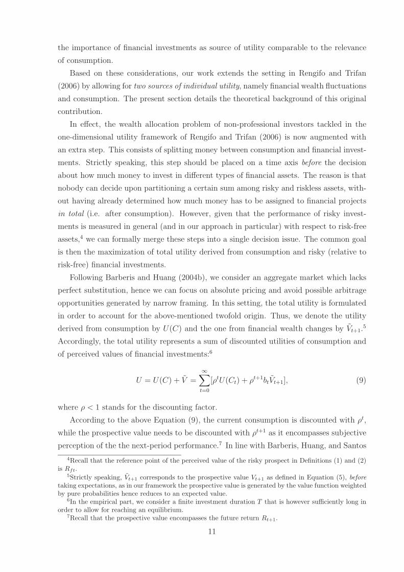
the current value of the risky investment St, as well as the amount of money borrowed

(Bt > 0) or lent (Bt < 0) are reformulated in order to correspond to the total wealth Wt,

that now also comprises consumption and yield:

θt =Wt − Ct + Bt

Wt − Ct

(12a)

St = θt(Wt − Ct) (12b)

Bt = (Wt − Ct)VaR∗ + VaR

(Wt − Ct)Rft − VaR. (12c)

Note that the post-consumption wealth fraction allocated to risk-free assets becomes

1 − θt = −Bt/(Wt − Ct). Also, the next period total results from the current financial

investment and can be expressed as:11

Wt+1 = (Wt − Ct)[θtRt+1 + (1 − θt)Rft]. (13)

Noting that the maximization in Equation (10) is carried out for both consumption Ct

and the wealth fraction invested in risky assets θt (hence the value of the risky investment

St), the corresponding Euler equations for optimality at equilibrium yield:12

ρRfE

[

(

Ct+1

Ct

)

−γ]

= 1 (14a)

ρE

[

Rt+1

(

Ct+1

Ct

)

−γ]

+ b0ρC−γt E[v(Gt+1)] = 1. (14b)

Moreover, E[v(Gt+1)] is identical to the prospective value at equilibrium that we denote

by V . Our goal is to then provide an empirical value for V according to Equation (6) for

the loss aversion parameter λ of the representative investor in equilibrium.

In order to perform the estimation of V , additional assumptions concerning the con-

sumption and return dynamics are needed. In line with Barberis and Huang (2004a),

Equations (68)-(70), we take:13

11A part Ct+1/Wt+1 is subsequently allocated to consumption, but consumption generates merelyutility and not wealth.

12See Equation (27), (28) from Barberis, Huang, and Santos (2001).13Note that Barberis, Huang, and Santos (2001) assume that returns develop following the dividends

payed by the risky asset Rt+1 = (Pt+1 + Dt+1)/Pt. If this can be considered as a sound assumptionon an annual basis, an annoying problem emerges in terms of higher portfolio evaluation frequencies.While prices vary daily, dividends are released only once every three months or even at longer timeintervals. (For instance, according to data from finance.yahoo.com, the mean frequency of dividendsreleases amounts to approximatively 4.5 months.) This generates a non-smooth dividend evolution thataccounts on one hand for the dates of dividend release (when dividends truly change in value) and, onthe other hand, for the in-between periods (when no dividends are distributed to investors, meaning they

13

log

(

Ct+1

Ct

)

= c + σcǫt+1 (15a)

log(Rt+1) = r + σrηt+1 (15b)(

ǫt+1

ηt+1

)

∼ N

((

0

0

)

,

(

1 σcr

σcr 1

))

, i.i.d. over time. (15c)

Thus, for a constant risk-free rate Rf the equilibrium Equations (14) entail:14

exp

(

−γc +γ2σ2

c

2

)

=1

ρRf

(16a)

exp

(

−γc + r +γ2σ2

c + σ2r

2− γσcr

)

+ b0C−γt V =

1

ρ. (16b)

2.2.2 The non-expected utility approach

Although the expected-utility maximization represents the most widespread theoretical

approach so far, Barberis, Huang, and Thaler (2003) claim there is another specifica-

tion that best captures the utility of decisions under risk. In particular, this is a non-

expected recursive utility with first-order risk aversion (R-FORA). Yet, simple R-FORA

specifications account merely for loss aversion and hence need to be extended in order

to accommodate with both narrow framing and loss aversion. These phenomena appear

to be crucial for explaining several stock market puzzles and constitute the core of our

approach. Henceforth we refer to the R-FORA setting with narrow framing as the non-

expected utility approach.

We rely on the approach proposed in Barberis and Huang (2004a) according to which

investors maximize a recursive utility-function Ut, that is defined as:

Ut = ⋄〈Ct, µ(Ut+1 + b0Et[v(Gt+1)]|It)〉, (17)

can be considered as constant from one trade to the other). Formally, between two successive dividendreleasing times (u, u + 1], we have:

Dt+1 =

{

Du, for t ∈ (u, u + 1)

Du+1, for t = u + 1,hence

Dt+1

Dt

=

1, for t ∈ (u, u + 1)Du+1

Du

, for t = u + 1.

14Here we used the fact that, for x ∼ N(µ, σ2), E[exp(x)] = exp(µ + σ2/2). Also, for xi ∼ N(µi, σ2i ),

where i = 1, 2 i.i.d. over time and with covariance σ12, E[exp(x1+x2)] = exp(µ1+µ2+(σ21 +σ2

2)/2+σ12).

14

where

⋄ 〈C, x〉 = [(1 − β)C1−γ + βx1−γ ]1

1−γ , for 0 < β < 1, 0 < γ 6= 1 (18a)

µ(x) = (E[x1−γ ])1

1−γ , for 0 < γ 6= 1 (18b)

Gt+1 = θt(Wt − Ct)(Rt+1 − Rft) (18c)

v(x) =

x, for x ≥ 0

λx, for x < 0, for λ > 1. (18d)

Here, ⋄(., .) is an aggregator function and µ the homogenous certainty equivalent of the

distribution of future utility conditional on the information It at time t, the next-period

value of the risky investment Gt+1, and the individual value function v.

We restrict our analysis to the general equilibrium for aggregate markets (with a

representative investor), in line with Equations (60)-(62) and the subsequent Example

6.1 for the stock market in Barberis and Huang (2004b). Our focus remains on non-

professional investors’ decisions concerning the wealth allocation among consumption,

the risky portfolio returning Rt, and the risk-free asset with the gross return Rft. When

a fraction θt of post-consumption wealth is invested in the risky portfolio and another

fraction, now of the total wealth, αt = Ct/Wt is consumed, the following (Euler) equations

yield necessary and sufficient conditions at equilibrium:

βRftEt

[

(

Ct+1

Ct

)

−γ]{

βEt

[

(

Ct+1

Ct

)

−γ

Rtot

t+1

]}γ

1−γ

= 1 (19a)

Et

[

(

Ct+1

Ct

)

−γ

(Rt+1 − Rft)

]

Et

[

(

Ct+1

Ct

)

−γ] + b0Rft

(

β

1 − β

)γ

1−γ(

1 − αt

αt

)

−γ

1−γ

Et[v(Rt+1 − Rft)] = 0

(19b)

Et

[

(

Ct+1

Ct

)

−γ

(Rtott+1 − Rft)

]

Et

[

(

Ct+1

Ct

)

−γ] + b0Rft

(

β

1 − β

)γ

1−γ(

1 − αt

αt

)

−γ

1−γ

θtEt[v(Rt+1 − Rft)] = 0,

(19c)

where Rtott+1 = θtRt+1 + (1 − θt)Rft is the total gross return of the combination between

risky and risk-free assets. Equation (19c) is derived from (19b) by multiplication with θt.

The next period financial wealth formulated in Equation (13) can be now rewritten as

15

Wt+1 = (Wt − Ct)Rtott+1. Thus,

Rtot

t+1 =αt

αt+1(1 − αt)

Ct+1

Ct

. (20)

Assuming time constancy for the portfolio wealth fraction θ, the consumption ratio α,

and the risk-free return Rf , the total gross return results in:

Rtot

t+1 =1

1 − α

Ct+1

Ct

⇒ log(Rtot

t+1) = − log(1 − α) + c + σcǫt+1. (21)

Thus, the equilibrium Equations (19) yield:

β1

1−γ (1 − α)−γ

1−γ RfE

[

(

Ct+1

Ct

)

−γ]{

E

[

(

Ct+1

Ct

)1−γ]}

γ

1−γ

= 1 (22a)

E

[

(

Ct+1

Ct

)

−γ

(Rt+1 − Rf )

]

E

[

(

Ct+1

Ct

)

−γ] + b0Rf

(

β

1 − β

)γ

1−γ(

1 − α

α

)

−γ

1−γ

E[v(Rt+1 − Rf )] = 0

(22b)

E

[

(

Ct+1

Ct

)

−γ

(Rtott+1 − Rf )

]

E

[

(

Ct+1

Ct

)

−γ] + b0Rf

(

β

1 − β

)γ

1−γ(

1 − α

α

)

−γ

1−γ

θE[v(Rt+1 − Rf )] = 0.

(22c)

We proceed similar to Section 2.2.1 by assuming the parameter dynamics of con-

sumption and returns in Equations (15). Also, we consider that the value functions

(1) and (2) are equivalent in expectation to the prospective value in Equation (5), i.e.

16

V = E[v(Rt+1 − Rf )]. Thus, the equilibrium Equations (22) can be further restated as:

β1

1−γ (1 − α)−γ

1−γ Rf exp

(

γσ2c

2

)

= 1 (23a)

− exp

(

−γc + r +γ2σ2

c + σ2r

2− γσcr

)

+ Rf exp

(

−γc +γ2σ2

c

2

)

= b0Rf

(

β

1 − β

)γ

1−γ(

1 − α

α

)

−γ

1−γ

exp

(

−γc +γ2σ2

c

2

)

V (23b)

−1

1 − αexp

(

(1 − γ)c +(1 − γ)2σ2

c

2

)

+ Rf exp

(

−γc +γ2σ2

c

2

)

= b0Rf

(

β

1 − β

)γ

1−γ(

1 − α

α

)

−γ

1−γ

exp

(

−γc +γ2σ2

c

2

)

θV . (23c)

3 Empirical results

This section presents empirical findings based on the theoretical framework presented in

the above Section 2.2. We start off by describing the general assumptions made in order

to facilitate the estimation procedure and to render the two settings with expected and

non-expected utility comparable. Subsequently, the estimation results are illustrated and

commented on for each of these settings, where the exposition focuses on two main aspects.

First, we address the evolution of the attitude towards financial losses as described by the

loss aversion coefficient and the extended measures LAi and gRA. Second, we examine

the optimal wealth allocation among consumption, risky, and riskless assets, as well as

the occurrence of myopic loss aversion.

3.1 General assumptions

Our estimations are based on the same data set as in Rengifo and Trifan (2006), that

includes the SP500 and the 10-year bond nominal returns (as proxies for the risky and

the risk-free investment, respectively) from 01/02/1962 to 03/09/2006 (11,005 daily ob-

servations). This data is divided into two parts, from which only the second one (from

03/01/1982 to 03/09/2006, specifically 6,010 observations) is considered to be the active

set (and used for performing simulations). The observations before the “date zero” of

the trade (03/01/1982) serve to estimate the empirical mean and the standard deviation

of the portfolio returns at date zero. Additionally, aggregate per-capita consumption

data between 01/02/1962 and 12/31/200515 provide a basis for the calculation of the

15This data was provided by the Department of Commerce, Bureau of Economic Analysis and Bureauof the Census.

17

log-consumption mean and variance.16 Note that this data set allows us to assess con-

sumption values corresponding to portfolio evaluations frequencies of merely one year and

three months. Thus, we cannot replicate the more detailed analysis in Rengifo and Trifan

(2006) regarding the impact of the evaluation frequency on investor decisions.

After smoothing out the outlier corresponding to the October 1987 market crash,17

quarterly and yearly returns are constructed from the active data set and used to derive

the optimal risky investment. In so doing, we assume that investors start by spreading

their wealth equally between consumption and financial assets, where the latter fraction

is further allocated equally to the risky portfolio and the bond. In addition, investors are

considered to be long-lived beyond the VaR-horizon and are not allowed to quit the market

during the trading period. Moreover, cushions are assumed to be cumulatively amassed

from past trades (starting at date zero) Zt =t∑

i=0

Si, portfolio gross returns to be normally

distributed, and future portfolio returns to be estimated as the unconditional mean of

past returns. In addition, we assess Rf = mean[Rft], c = mean[log(Ct+1) − log(Ct)] in

Equation (15a), and r = mean[log(Rt)] in Equation (15b), where the means are computed

throughout the active period (from 03/01/1982 to 03/09/2006).

A delicate issue that might emerge from our consideration that investors are long-

lived investors and have financial investments as sole source of wealth,18 forces us to make

a final and more specific assumption. It is possible that financial investments do not

generate sufficient revenues in order to cover investors’ consumption needs over the entire

investment interval. We attempt to circumvent this potential problem19, by considering

that at each time t investors dispose of additional incomes It. Such incomes represent, for

instance, the wages earned by non-professional investors from their main employment.20

These incomes are considered as exogenous, that is, they stem from outside of those

investments that constitute the decision making object at hand. Under this assumption,

the total wealth Wt in Equation (13) results from both financial investments and the

16Descriptive statistics can be found in Table 7 in Appendix 5.1.17This outlier is replaced with the mean of the ten before and after data points18Recall that both consumption and financial investments generate utility, yet only the latter is “pro-

ductive” and can effectively augment wealth.19Note that Barberis and Huang (2004a,b) avoid this problem by fixing the percentage of post-

consumption wealth invested in risky assets θ. We do not consider this as appropriate in our frameworkfor two reasons. First, Barberis and Huang (2004a,b) exclusively work with non-expected utility, whileour aim is to render comparable two approaches, namely those with expected and non-expected utility.Second, our model rests on the idea that θ depends on the subjective VaR* (see Equations (12)). Hence,imposing constancy on this parameter would eliminate the whole analyzed mechanism of how individualperceptions of financial investments reflect in the wealth allocation.

20As their name indicates, non-professional investors mainly earn their living from other activities(developed for example as employees of a company) than from financial investments. The latter merelyrepresent a secondary source of revenues.

18

additional income It and yields:

Wt+1 − It+1 = (Wt − Ct)[θtRt+1 + (1 − θt)Rft]. (24)

We assume that the additional income covers a part of the consumption needs of the

current period and set:21

It =Ct

αδ, (25)

where α represents the percentages of total wealth dedicated to consumption in the equi-

librium of the non-expected utility setting and δ > 0 is an arbitrary constant. Apparently,

for δ ≤ 1/α (δ > 1/α) the extra income exceeds (does not entirely meet) the consumption

needs of the period It ≥ Ct (It < Ct). We distinguish two particular cases with no prac-

tical meaning in the present framework. First for δ = 1, the current extra income yields

a fraction of the consumption needs It = Ct/α and investors should assign no money to

financial assets in total Rtott+1 = 0.22 Second, for δ = 1/α the extra income that covers

exactly the current consumption It = Ct. As the total financial investment then becomes

independent of α, Rtott+1 = Ct+1/Ct, there is no further connection between investment de-

cisions and the subjective perception of financial investments in the non-expected utility

equilibrium.23 Consequently, we henceforth set δ ∈ R+ \ {0, 1, 1/α}.24

We close this section by detailing the values of the behavioral parameters that underlie

our simulations. First, we chose different values of the initial coefficient of loss aversion λ,

namely in the set {0.5; 1; 2.25; 3}. The value of 2.25 recommended by the prospect theory

is considered as the standard case and is mainly referred to in the text. Second, we consider

different values of the additional income It. As α depends on β according to Equations

(22), the choice of β and further of δ dictate the evolution of the additional income. Thus,

we take β ∈ {0.2; 0.5; 0.8} and δ ∈ {0.6; 0.7; 0.8; 0.9}.25 Our subsequent comments usually

21This assumption permits an easy formal manipulation and ensures the comparability of the twoapproaches. At the same time, it allows for sufficient flexibility with respect to the choice of the incomemagnitude.

22Moreover, in this case the percentage of post-consumption wealth assigned to risky assets in equilib-rium from Equation (29b) yields: θ = Rf/[Rf − exp(r + σ2

r/2 − γσcr)] ≥ 1. This induces investors tothrow caution to the wind, borrowing ever more money , which is then channelled into the risky portfolio.

23Recall first that V relies on subjective perceptions and is derived on the basis of behavioral parametersaccording to Equation (5). Then this connection is ensured by the interdependency of α and V fromEquations (29). It is central to our work, as we assume that all decisions rely on individual perceptionsand attempt to analyze how they change subject to different perception parameters. For δ = 1/α,the percentage of post-consumption wealth allocated to risky assets in equilibrium from Equation (29b)becomes independent of α, specifically θ = [Rf − exp(c + (1 − 2γ)σ2

c/2)/[Rf − exp(r + σ2r/2 − γσcr)].

24Note that for the purpose of comparability, we consider identical additional incomes in both settingswith expected and non-expected utility.

25We actually run simulations for all β ∈ {0.2; 0.5; 0.8; 0.98} and δ ∈{0.2; 0.5; 0.6; 0.7; 0.8; 0.9; 2; 10; 100}. The final choice of the value-ranges mentioned in the text ismotivated by several facts and findings. First, δ > 1 entails negative values for the wealth percentages tobe consumed in the expected-utility setting. Second, the value β = 0.98, which is in line with Barberisand Huang (2004b), yields implausible (that is negative) estimates of the same percentages in the

19

account for all considered (β, δ)-combinations. Yet the results illustrated in the tables of

Sections 3.2 and 3.3 focus on the case with δ = 0.9 and consider two different values of

β = 0.2 and β = 0.8. This allows us to compare the reactions of investors who perceive one

of the two utility sources (namely the consumption for β = 0.2 and the financial wealth

fluctuations for β = 0.8) as dominant. All unreported numerical results are available upon

request.

3.2 The expected-utility approach

In order to estimate the variables of interest in our model, we start by considering the

expected-utility setting. Following Barberis, Huang, and Santos (2001) and Barberis and

Huang (2004a), we chose three values of the parameter γ that express different degrees of

the risk aversion of the consumption utility, namely γ ∈ {0.5; 1; 1.5}. In line with the same

papers, we also account for no and moderate influence of past losses on the perception

of risky investments and set k ∈ {0; 3}. In addition, we consider different degrees of

narrow framing, specifically b0 ∈ {0.001; 100; 1, 000} for γ ≥ 1, and b0 ∈ {0.001; 5; 10} for

γ < 1.26 Finally, recall that in order to make the expected-utility setting comparable to

the non-expected utility one in Section 3.3, we consider that investors dispose of periodical

additional incomes. The magnitude of these incomes is dictated by a free-choice parameter

δ and by a behavioral parameter β that is specific to the non-expected utility setting. As

β stems from the non-expected utility framework, it has no intuitive meaning in the

present setting with expected utility. Thus, we subsequently interpret the variation of our

equilibrium estimates with respect to the changes in the additional income It (instead of

the changes in β). This is possible, as It increases (decreases) subject to higher β (δ)-

values.27 In essence, higher additional incomes are equivalent to more relaxed requirements

for financial investments.

Equation (16a) delivers an estimate of the discounting factor ρ in the aggregate equi-

librium.28 Plugging this estimate ρ into Equation (16b), we obtain an empirical equivalent

for the prospective value in equilibrium V . We can further assess the corresponding loss

non-expected equilibrium.26First, in light of Equation (26), b0 6= 0. Second, recall that the weighting coefficient of the utility

derived from risky investments in Equation (10) is obtained by multiplying the narrow framing parameterb0 with the aggregate consumption C−γ

t . Consequently, as mean[Ct] ≈ 46, 000 in our sample, yet thehighest b0 = 1, 000 entails for γ = 1 a still small (non-discounted) contribution of this source of utilityto the total utility, specifically of less than 2.2%. Similarly, b0 = 10 and γ = 0.5 result in a share of lessthan 4.7%.

27Due to our assumption that It = Ct/(αδ) and according to α = 1− β1

γ R1−γ

γ

f exp(1−γ)σ2

c

2 in Equation(29a).

28Of course, we could also fix ρ and estimate γ. However, this procedure proves to be more delicate,given that Equation (16a) is a second-order equation in γ, such that the existence and number of realroots depends on the sign of its determinant c2 − 2σ2

c log(ρRf ). In the case with either none or twodistinct real solutions, we cannot provide an economic interpretation of the equilibrium.

20

aversion coefficient λ according to Equation (6). In particular, the explicit expressions of

the desired variables are based on the following reformulation of the equilibrium Equations

(16):

ρ =1

Rf

exp

(

γc −γ2σ2

c

2

)

(26a)

V =Cγ

t

b0

[

1

ρ− exp

(

−γc + r +γ2σ2

c + σ2r

2− γσcr

)]

. (26b)

Unreported results show that in the absence of narrow framing (as approximated by

the case with the lowest b0 = 0.001), the estimates of the loss aversion coefficient λ are

highly negative (positive) for yearly (quarterly) portfolio revisions, and thus implausible.

In effect, the individual attitude to losses stemming from financial investments has no

practical meaning (and is difficult to interpret in terms of our model) when investors pay

no attention to the utility derived from these investments compared to the consumption

utility. Similarly, an excessive consumption-based risk aversion γ = 1.5 results in im-

plausible estimates of both ρ (that are slightly supra-unitary) and in part of λ (that are

negative or too highly positive, with the exception of the case with b0 = 1000), as intu-

itively expected according to Equations (26). In sum, plausible parameter combinations

for reaching the aggregate market equilibrium in the expected-utility setting turn out to

be (γ = 0.5, b0 ∈ {5; 10}) and (γ = 1, b0 ∈ {100; 1000}) and they are addressed below.

Table 1 (Table 8 in Appendix 5.2) presents the estimation results for these parameter

combinations, yearly (quarterly) portfolio evaluations in our usual cases with λ = 2.25,

δ = 0.9, and β ∈ {0.2; 0.8}. Recall that the switch from β = 0.2 to β = 0.8 for a fixed

δ = 0.9 is equivalent with (hence interpreted as) an increase in additional incomes.

21

β = 0.8 β = 0.2γ = 0.5 γ = 1 γ = 0.5 γ = 1

k = 0 k = 3 k = 0 k = 3 k = 0 k = 3 k = 0 k = 3b0 = 5

ρ 0.95685 0.95685 0.98208 0.98208 0.95685 0.95685 0.98208 0.98208

V -92.17895 -92.17895 -23,107.54900 -23,107.54900 -92.17895 -92.17895 -23,107.54900 -23,107.54900

λ 1.0853 1.0836 0.71912 0.70696 0.79627 0.99587 -2.56203 3.17835b0 = 10

ρ 0.95685 0.95685 0.98208 0.98208 0.95685 0.95685 0.98208 0.98208

V -46.08948 -46.08948 -11,553.77500 -11,553.77500 -46.08948 -46.08948 -11,553.77500 -11,553.77500

λ 1.0867 1.0851 0.90059 0.89201 0.79024 0.99968 -0.65440 1.96148b0 = 100

ρ 0.95685 0.95685 0.98208 0.98208 0.95685 0.95685 0.98208 0.98208

V -4.60895 -4.60895 -1,155.37750 -1,155.37750 -4.60895 -4.60895 -1,155.37750 -1,155.37750

λ 1.08792 1.08635 1.0639 1.0585 0.78480 1.00311 1.0625 0.86629b0 = 1, 000

ρ 0.95685 0.95685 0.98208 0.98208 0.95685 0.95685 0.98208 0.98208

V -0.46089 -0.46089 -115.53775 -115.53775 -0.46089 -0.46089 -115.53775 -115.53775

λ 1.08804 1.08648 1.0802 1.0752 0.78426 1.00345 1.2341 0.75677

Table 1: The main estimated parameters in the expected-utility setting for yearly data, λ = 2.25 and δ = 0.9.

22

We first address the investors’ attitude towards financial losses. One variable that

captures this attitude is the loss aversion coefficient, the equilibrium estimates of which

are denoted by λ. From Tables 1 and 8 we observe that for higher additional incomes

(formally corresponding to β = 0.8), λ takes values slightly above 1 for both yearly and

quarterly portfolio evaluations. As 1 can be considered to be the “neutral” loss-aversion

value, our representative investor appears to be rather indifferent between financial gains

and losses.

Surprisingly, lower extra-money dedicated to consumption (β = 0.2) entails a decrease

in the loss aversion coefficient in equilibrium. This variation is confirmed for further

δ-values. At first glance, this conclusion appears to be counterintuitive. Accordingly,

investors who are less sure of being able to cover current consumption needs (as their

additional incomes are lower) become more relaxed towards financial losses (although such

losses would reduce their revenues even more). One possible explanation is that agents

tend toward taking the chance of investing in financial assets, as this chance (in other words

gambling) hides not only the danger of losses, but also the promise of gains. However,

note that the loss aversion coefficient is not a one-to-one measure of investor actions

concerning wealth allocation. They represent the result of more complex phenomena.

Thus, variations of the loss aversion coefficient due to changes in the additional income

do not need to be proportionally reflected in the magnitude of the actual investment in

financial assets. For instance, Tables 3 and 10 show that the lower additional incomes

corresponding to β = 0.2 entail smaller fractions of the total wealth allocated to risky

assets (1− C/W )θ. More detailed investigations referring to this issue are undertaken at

the end of this section. Finally, note also that the loss aversion coefficient might be an

imperfect measure of the attitude towards financial losses. Yet, the other two measures

LAi and gRA do not appear to evolve differently (see the findings in this respect presented

later in this section).

In general, λ does not reach the value of 2.25 suggested in the original prospect theory

for any of the considered parameter configurations.29 This is not very surprising, as the

latter has been mostly obtained in experiments where subjects are faced only with financial

decisions. Our results underline the fact that, when accounting for both consumption

and financial investments as generators of individual utility, investor reluctance towards

financial losses measured by the equilibrium-equivalent loss aversion coefficient λ is lower.

On average, λ is somewhat smaller when portfolios are evaluated more often. At first

glance, this appears to be at odds with the idea of myopic loss aversion. However, two

remarks can be made in this regard. First, note that the myopic loss aversion originates

in, but is not measured by, the loss aversion coefficient. A more appropriate measure is

29One of the highest values, λ = 1.782, is obtained for β = 0.2, δ = 0.7, k = 0, and yearly evaluations.

23

the wealth fraction allocated to risky assets, the evolution of which will be subsequently

detailed.30 Second, the observed changes in λ are rather small, especially for incomes

corresponding to β ≥ 0.5. This points to a relative stability of the loss attitude in

equilibrium with respect to the portfolio evaluation frequency for a higher certitude of

covering current consumption needs (namely for middle-range to high additional incomes).

Moreover, for a fixed degree of narrow framing b0, the variable λ resulting for the

higher additional income corresponding to β = 0.8, appears to decrease when switching

from k = 0 to k = 3. Note also that the respective changes in value are very small

for quarterly portfolio evaluations although the inverse holds for λ = 2.25, β = 0.2

and γ = 0.5. This tendency is confirmed for most of the other considered parameter

combinations, where the differences become substantial for low values of both β and δ.31

However, we can conclude that when the additional income to be consumed is sufficiently

high (β ≥ 0.5), the reluctance towards past losses does not have a significant impact on

the attitude towards current losses. It is still difficult to formulate clear-cut conclusions

with respect to the variation of λ subject to the narrow framing coefficient b0 when k is

fixed. For the highest additional income values (β = 0.8), we notice a slight tendency to

increase (decrease) when portfolios are evaluated once a year (every three months), the

changes being yet very small.

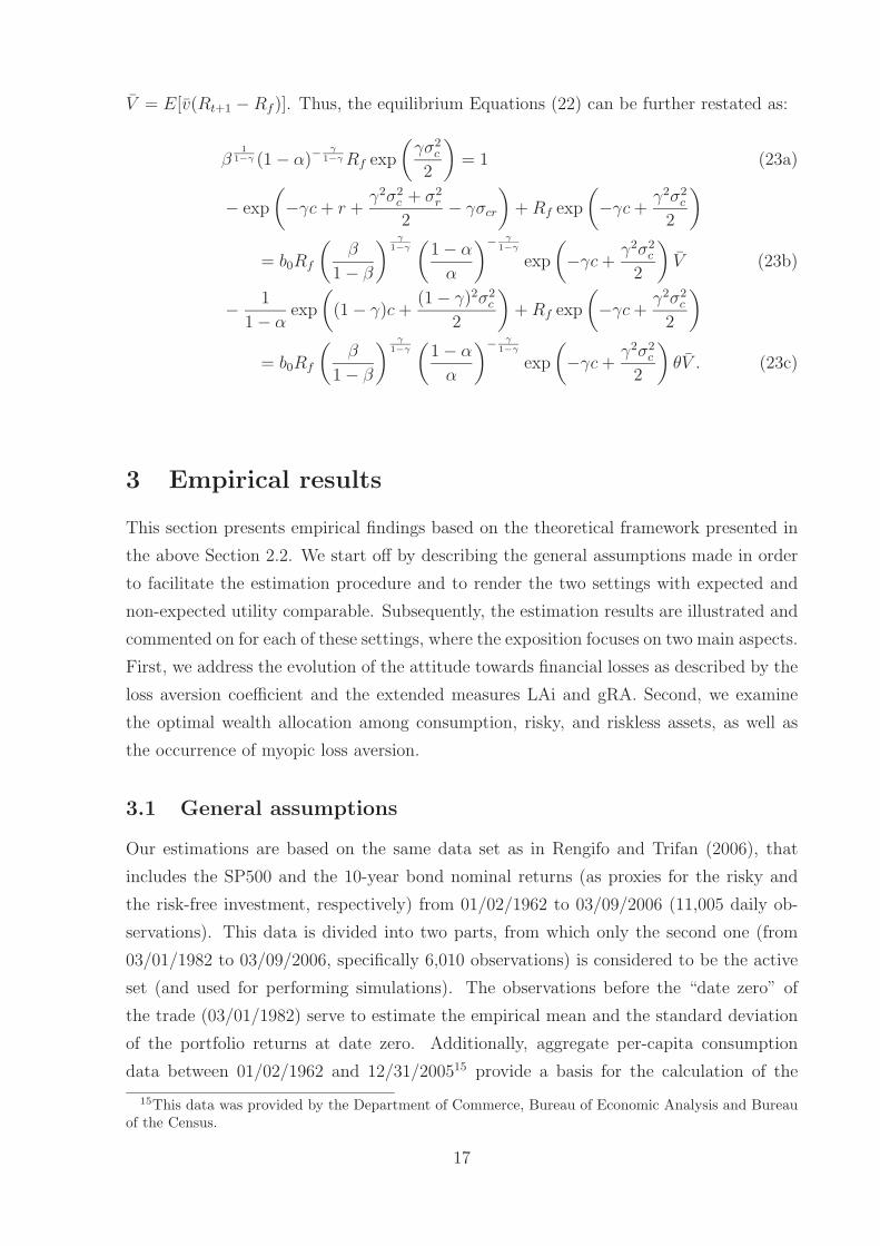
In the same context of the investor attitude towards financial losses, it is interesting

to follow the evolution of the two other measures introduced in the theoretical section,

namely LAi in Equation (7) and gRA in Equation (8). Table 2 (Table 9 in Appendix 5.2)

presents the corresponding estimates for yearly (quarterly) portfolio evaluations and the

cases already analyzed in Table 1 (Table 8) above.

30This remark is in the same spirit as the above comments on the variation of λ subject to β.31Specifically, one of the biggest differences is obtained for β = 0.2 and δ = 0.7, where λ decreases for

k = 3 to almost one half of the value for k = 0.

24

β = 0.8 β = 0.2γ = 0.5 γ = 1 γ = 0.5 γ = 1

k = 0 k = 3 k = 0 k = 3 k = 0 k = 3 k = 0 k = 3b0 = 5LAi 1.0853 1.0408 0.7191 0.6641 0.79627 0.95421 -2.562 3.1365gRA 2,375,552.2 2,086,117.3 4,047,794.6 3,553,753.8 288,130 249,340 371,530 428,830

b0 = 10LAi 1.0867 1.0423 0.9006 0.8491 0.79024 0.95801 -0.6544 1.9196gRA 2,375,720.2 2,086,278.7 4,089,066.7 3,591,723.6 288,100 249,450 433,480 422,590

b0 = 100LAi 1.0879 1.0436 1.0639 1.0157 0.7848 0.96144 1.0625 0.82444gRA 2,375,871.4 2,086,423.9 4,126,211.6 3,625,896.5 288,080 249,540 489,230 416,970

b0 = 1, 000LAi 1.0880 1.0437 1.0802 1.0323 0.78426 0.96178 1.2341 0.71492gRA 2,375,886.5 2,086,438.4 4,129,926.1 3,629,313.8 288,070 249,550 494,810 416,410

Table 2: The estimated index of loss aversion (LAi) and global first-order risk aversion (gRA) in the expected-utility setting for yearlydata, λ = 2.25 and δ = 0.9.

25

For the most part, the evolutions of LAi and gRA confirm the conclusions reached

so far for λ. That is, both measures of the attitude towards financial losses increase

for enhanced narrow framing, decrease when past losses are penalized, and also diminish

when portfolio performance is checked more often (where the changes in gRA are very

high), other things being equal.

Moreover, LAi closely follows the values of the simple loss aversion coefficient in the

market equilibrium, being somewhat (but almost always insignificantly) lower. We cannot

yet detect a clear pattern of its variation with the additional income. In this regard, gRA

behaves more consistently, as it clearly increases for higher additional incomes (specifically,

for either higher β or lower δ-values).32 Also, gRA better describes how the reluctance to

losses extends across time, as it clearly drops when k increases from zero to three. In sum,

gRA appears to better capture the changing attitude to losses in equilibrium subject to

the variation of different model parameters.

Before approaching the problem of optimal wealth allocation, we investigate the other

two variables for which estimates can be obtained in the expected-utility equilibrium.

Tables 1 and 8 contain the respective values for the usual cases with δ = 0.9 and β ∈

{0.2; 0.8}. As apparent from Equation (26a), the discounting factor ρ does not depend

on the choice of either β, or δ, or b0. Table 1 shows that for yearly portfolio evaluations

and γ = 1, ρ ≈ 0.98, which complies with the assumptions of Barberis, Huang, and

Santos (2001) and Barberis and Huang (2004a). As expected, lower consumption-based

risk aversion γ = 0.5 entails lower preference for immediacy and our estimate ρ < 0.96.

The corresponding estimates from Table 8 for quarterly portfolio revisions are somewhat

higher and less sensitive to changes in γ.

Finally, note that the estimated prospective value in equilibrium remains negative

V < 0 across all considered parameter configurations. Thus, financial investments appear

to lower the overall utility of our representative investor. The evolution of V for different

parameter combinations confirms the tendencies pointed out for λ. In particular, inde-

pendently of the penalty on past losses k, V increases subject to higher narrow framing

b0, as well as for more frequent portfolio evaluations, other things being equal.

In the sequel, we turn to the question of whether or not myopic loss aversion becomes

manifest in our equilibrium setting with two-dimensional expected utility. The answer

goes hand in hand with the wealth allocation in equilibrium. The subsequent comments

refer to the findings for all considered additional income configurations (or all (β, δ)-

combinations), while direct references to the values in Tables 3 and 10 are explicitly

indicated.

In this context, we compute the mean of the proportions of total wealth dedicated to

32Recall that higher gRA-values point to lower aversion to financial losses.

26

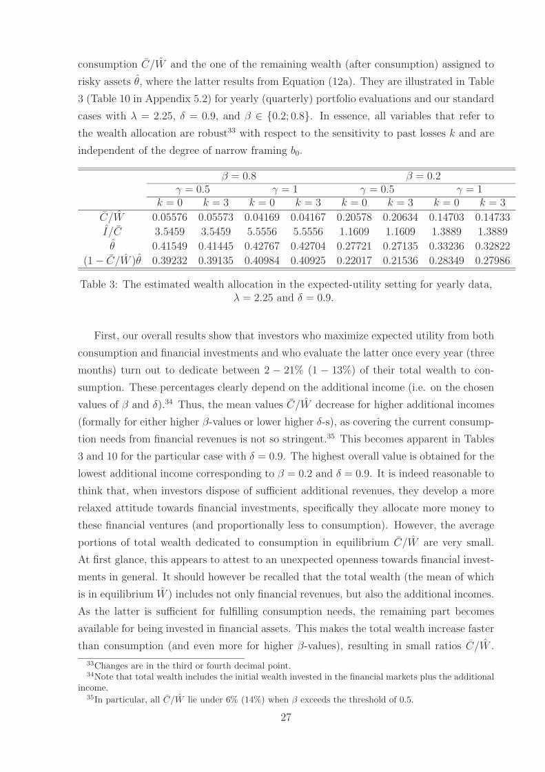
consumption C/W and the one of the remaining wealth (after consumption) assigned to

risky assets θ, where the latter results from Equation (12a). They are illustrated in Table

3 (Table 10 in Appendix 5.2) for yearly (quarterly) portfolio evaluations and our standard

cases with λ = 2.25, δ = 0.9, and β ∈ {0.2; 0.8}. In essence, all variables that refer to

the wealth allocation are robust33 with respect to the sensitivity to past losses k and are

independent of the degree of narrow framing b0.

β = 0.8 β = 0.2γ = 0.5 γ = 1 γ = 0.5 γ = 1

k = 0 k = 3 k = 0 k = 3 k = 0 k = 3 k = 0 k = 3

C/W 0.05576 0.05573 0.04169 0.04167 0.20578 0.20634 0.14703 0.14733

I/C 3.5459 3.5459 5.5556 5.5556 1.1609 1.1609 1.3889 1.3889

θ 0.41549 0.41445 0.42767 0.42704 0.27721 0.27135 0.33236 0.32822

(1 − C/W )θ 0.39232 0.39135 0.40984 0.40925 0.22017 0.21536 0.28349 0.27986

Table 3: The estimated wealth allocation in the expected-utility setting for yearly data,λ = 2.25 and δ = 0.9.

First, our overall results show that investors who maximize expected utility from both

consumption and financial investments and who evaluate the latter once every year (three

months) turn out to dedicate between 2 − 21% (1 − 13%) of their total wealth to con-

sumption. These percentages clearly depend on the additional income (i.e. on the chosen

values of β and δ).34 Thus, the mean values C/W decrease for higher additional incomes

(formally for either higher β-values or lower higher δ-s), as covering the current consump-

tion needs from financial revenues is not so stringent.35 This becomes apparent in Tables

3 and 10 for the particular case with δ = 0.9. The highest overall value is obtained for the

lowest additional income corresponding to β = 0.2 and δ = 0.9. It is indeed reasonable to

think that, when investors dispose of sufficient additional revenues, they develop a more

relaxed attitude towards financial investments, specifically they allocate more money to

these financial ventures (and proportionally less to consumption). However, the average

portions of total wealth dedicated to consumption in equilibrium C/W are very small.

At first glance, this appears to attest to an unexpected openness towards financial invest-

ments in general. It should however be recalled that the total wealth (the mean of which

is in equilibrium W ) includes not only financial revenues, but also the additional incomes.

As the latter is sufficient for fulfilling consumption needs, the remaining part becomes

available for being invested in financial assets. This makes the total wealth increase faster

than consumption (and even more for higher β-values), resulting in small ratios C/W .

33Changes are in the third or fourth decimal point.34Note that total wealth includes the initial wealth invested in the financial markets plus the additional

income.35In particular, all C/W lie under 6% (14%) when β exceeds the threshold of 0.5.

27

The coverage rate of consumption from additional incomes is on average reflected by the

ratio I/C, the evolution of which can be observed in the same Tables 3 and 10 for δ = 0.9.

In this case, the additional income covers on average more than the consumption needs,

as I/C > 1.36

Second, between 27 − 45% (2 − 17%) of the remaining wealth after consumption is

allocated to risky assets when yearly (quarterly) portfolio checks are performed. These

percentages correspond to the estimates θ derived across all considered parameter con-

figurations. The values of θ grow with the magnitude of the additional income (namely

subject to higher β or to lower δ-values).37 As stressed above, when investors have more

money at their disposal, they may also allocate higher sums to risky assets. Note that

the estimated percentages of post-consumption wealth invested in the risky portfolio are

lower than the respective values found in the one-dimensional utility setting in Rengifo

and Trifan (2006)38, where the estimates θ obtained for high β coupled with low δ-values

come closest. Again, the mean θ is not significantly different when investor penalize or

not past losses.

Finally, recall that while in the one-dimensional setting the total wealth is exclu-

sively assigned to financial investments, in the present two-dimensional setting θ stands

for percentages of post-consumption wealth invested in risky assets. The corresponding

percentages of total wealth assigned to risky investments can be obtained by multiplying

(1 − C/W ) by θ. Across all considered additional income values, θ amounts to between

approximately 22 − 43% (2 − 17%) for yearly (quarterly) portfolio evaluations. They are

higher for a more pronounced consumption-based risk aversion γ, for higher extra incomes

(which is equivalent to higher β and/or lower δ-values), and for more frequent portfolio

evaluations. These conclusions are illustrated for the case with δ = 0.9 in the same Ta-

bles 3 and 10. We can hence conclude that myopic loss aversion continues to manifest

when consumption is incorporated as an additional source of utility besides financial in-

vestments and when expected utility is maximized. In particular, investors remain highly

averse towards financial risks and their reluctance increases for more frequent evaluations

of the risky portfolio. In addition, the reluctance towards risky assets is more pronounced

than in the one-sided utility framework in Rengifo and Trifan (2006), and as expected,

grows as the additional income covers less of the current consumption needs.

We close this section with several remarks concerning the result replication for further

36For all considered δ < 1-values, I/C lies in the interval 1.16 − 8.33 for both frequencies of the risky-performance evaluations. The respective values increase for (higher β, lower δ)-combinations, as well asfor γ = 1.

37In particular, all values lie above 34% (14%) when β crosses over the neutral value of 0.5.38According to Table 1 in Rengifo and Trifan (2006), for cumulative cushions and normally distributed

expected returns they find that 49% (18.5%) of wealth is invested in risky assets when portfolios areevaluated yearly (quarterly).

28

values of the initial loss-aversion coefficient λ. Recall that this coefficient is employed in

order to derive VaR* from Equation (3) and the prospective value from Equation (5),

and the main analysis conducted so far relies on λ = 2.25. We run further sensitivity

tests for λ ∈ {0.5; 1; 3}, the results of which show that all evolution patterns found

above remain valid. While neither the estimated discounting factor ρ nor the derived

prospective value V depend on the initial loss-aversion coefficient, the equivalent λ varies

as expected, proportionally to λ. Moreover, the equilibrium-equivalent estimates of LAi

and gRA increase in λ, where the variations of LAi are rather minor but those of gRA

more pronounced. Naturally, the initial attitude towards losses should be proportionally

reflected in the attitude of the representative investor, required in order to reach the

aggregate equilibrium. Furthermore, the mean percentages of total wealth dedicated to

consumption in equilibrium C/W are rather robust with respect to the initial coefficient

of loss aversion. The percentages of post-consumption wealth invested in risky assets θ

slightly increase in λ, but the changes are already minor for λ ≥ 1. The same holds for

the resulting percentages of total wealth dedicated to risky investments (1−C/W )θ. This

suggests that investors who are initially more averse to financial losses and maximize two-

dimensional expected utility may exhibit slightly enhanced reluctance towards financial

investments in general, and towards risky investments in particular.

3.3 The non-expected utility approach

In order to derive parameter estimates in the equilibrium setting with non-expected utility,

we proceed analogously to Section 3.2. We again follow Barberis, Huang, and Santos

(2001) and Barberis and Huang (2004a), as well as our model restrictions in Equations

(18a) and (18b), and choose the risk aversion parameter of the consumption utility γ ∈

{0.5; 1.5}39 and the sensitivity to prior losses k ∈ {0; 3}. Given the particular form of

Equation (18a), the contribution of the risky prospect to the total utility decreases in the

narrow-framing coefficient b0 for γ > 1, such that we now take b0 ∈ {0.001; 0.01; 0.1; 0.5; 1}.

Under the assumption of periodical additional incomes of It = Ct/(αδ), the total gross

return from financial investments in Equation (21) results in:

Rtot

t+1 =1

1 − α

Ct+1 − αIt+1

Ct

=1

1 − α

δ − 1

δ

Ct+1

Ct

⇒ log(Rtot

t+1) = log(δ − 1) − log(δ) − log(1 − α) + c + σcǫt+1.

(27)

39Recall that according to Equation (18a), γ 6= 1.

29

Consequently, the equilibrium Equation (23c) changes to:

−δ − 1

δ(1 − α)exp

(

(1 − γ)c +(1 − γ)2σ2

c

2

)

+ Rf exp

(

−γc +γ2σ2

c

2

)

= b0Rf

(

β

1 − β

)γ

1−γ(

1 − α

α

)

−γ

1−γ

exp

(

−γc +γ2σ2

c

2

)

θV .

(28)

Thus, for a fixed subjective weight β in the aggregator function in Equation (18a),

Equations (23a), (23b), and (28) deliver estimators for the percentages of total wealth

dedicated to consumption α, the portion of post-consumption wealth invested in risky

assets θ and the prospective value V in equilibrium.40 Specifically, dividing Equations

(23b) and (28) and plugging the result into Equation (23a), we derive α and θ. Finally,

we restate Equation (23b) in order to obtain an expression for V . This yields the following

expressions of the parameters that can be estimated in the equilibrium of the non-expected

utility setting:

α = 1 − β1

γ R1−γ

γ

f exp

(

(1 − γ)σ2c

2

)

(29a)

θ =

Rf −δ − 1

δ(1 − α)exp

(

c +(1 − 2γ)σ2

c

2

)

Rf − exp

(

r +σ2

r

2− γσcr

)

=

δβ1

γ R1

γ

f − (δ − 1) exp

(

c −γσ2

c

2

)

δβ1

γ R1−γ

γ

f

[

Rf − exp

(

r +σ2

r

2− γσcr

)] (29b)

V =1

b0Rf

[

αβ

(1 − α)(1 − β)

]

−γ

1−γ[

Rf − exp

(

r +σ2

r

2− γσcr

)]

=1

b0

β(1 − β)γ

1−γ exp

(

γσ2c

2

) Rf − exp

(

r +σ2

r

2− γσcr

)

[

1 − β1

γ R1−γ

γ

f exp

(

(1 − γ)σ2c

2

)]

γ

1−γ

. (29c)

Note that in Equation (29b), the percentage of post-consumption wealth invested in risky

assets in equilibrium θ is inversely proportional on each additional income parameter δ and

the total-wealth percentage dedicated to consumption in equilibrium α. Then, according

to Equation (29a) and to our assumption It = Ct/(αδ), θ increases c.p. for higher weights

β, as well as for higher δ-values. Henceforth, we refer high β-values as the case where

40Again, it is possible to proceed in the opposite way: by fixing α and θ, an estimator for γ can bederived from Equation (23a). However, the double or possible non-real roots of quadratic equations aredifficult to interpret from an economical point of view. Equation (23a) has real roots if and only ifβRf ≥ exp(−(2 log(1 − α) + 2rf − σ2

c )2/(8σ2c )).

30

investors consider the utility derived from narrowly framed financial investments more

important than the consumption utility, according to the aggregator function in Equation

(18a).41

Unreported results show that an extreme consumption-based risk aversion γ = 1.5

again yields implausible values of the equilibrium estimates V and λ. Consequently, our

subsequent comments focus on the case with γ = 0.5. Table 4 (Table 11 in Appendix

5.3) presents the estimates from Equations (29) for yearly (quarterly) evaluations and our

standard cases with λ = 2.25, δ = 0.9, and β ∈ {0.2; 0.8}.

β = 0.8 β = 0.2k = 0 k = 3 k = 0 k = 3

b0 = 0.001α 0.31335 0.31335 0.95708 0.95708

θ -0.6726 -0.6726 -2.0563 -2.0563

V -943.98 -943.98 -309.06 -309.06

λ 1.0537 1.0502 0.83444 0.97344b0 = 0.01

α 0.31335 0.31335 0.95708 0.95708

θ -0.6726 -0.6726 -2.0563 -2.0563

V -94.398 -94.398 -30.906 -30.906

λ 1.0846 1.0829 0.78922 1.0005b0 = 0.1

α 0.31335 0.31335 0.95708 0.95708

θ -0.6726 -0.6726 -2.0563 -2.0563

V -9.4398 -9.4398 -3.0906 -3.0906

λ 1.0877 1.0861 0.7847 1.0032b0 = 0.5

α 0.31335 0.31335 0.95708 0.95708

θ -0.6726 -0.6726 -2.0563 -2.0563

V -1.888 -1.888 -0.61811 -0.61811

λ 1.088 1.0864 0.7843 1.0034b0 = 1

α 0.31335 0.31335 0.95708 0.95708

θ -0.6726 -0.6726 -2.0563 -2.0563

V -0.94398 -0.94398 -0.30906 -0.30906

λ 1.088 1.0865 0.78425 1.0035

Table 4: The main estimated parameters in the non-expected utility setting for yearlydata, λ = 2.25, γ = 0.5 and δ = 0.9.

We first note that similarly to the expected-utility findings, the prospective value

41Recall however that the weights of financial wealth in the (final) utility function are also influencedby the narrow framing coefficient, as apparent from Equation (17). However, β gives a clearer and morereadily interpretable picture of how investors balance between consumption and financial utility.

31

estimates V < 0 (and this across all considered parameter configurations). This reinforces

the idea that maximizers of two-dimensional utility perceive financial investments as one

that deteriorates the overall utility in the market equilibrium. However, V substantially

increases subject to the intensity of narrow framing. Naturally, investors who narrow-

frame financial investments perceive risky investments as more favorable or, equivalently,

as less destructive for the total utility.

Regarding the attitude towards financial losses, we first note that the estimates λ of

the loss aversion coefficient in equilibrium lie very close to the respective estimates in the

expected-utility setting.42 It is also interesting to observe that switching between (almost)

no narrow framing b0 = 0.001 to narrow framing b0 > 0.001 entails substantial variations

in λ. By contrast, in the presence of narrow framing b0 > 0.001 the loss aversion coefficient

does not significantly vary subject to the degree of narrow framing. This supports the

findings under expected-utility maximization that the absence of narrow framing with

respect to financial projects cannot impact the aversion towards financial losses.

Interestingly, the estimates λ slightly diminish for more frequent portfolio evaluations

and in the presence of narrow framing b0 > 0.001, but only as long as financial investments

are perceived as the main utility source β = 0.8. When, on the contrary, consumption

receives the highest weight in the utility aggregation as β = 0.2, this tendency is reverted.

Thus, more frequent checks of the risky-portfolio performance appear either to compensate

for or to enhance the loss aversion in equilibrium, depending on the importance that is

subjectively ascribed to financial utility relative to consumption utility.

Again, all obtained estimates λ lie below the originally proposed value of the loss

aversion coefficient 2.25. For yearly evaluations they are slightly higher (lower) than

the “neutral” value of 1, as β = 0.8 (β = 0.2). The highest value of λ is obtained for

β = 0.5, δ = 0.9, and k = 3.43 Accordingly, investors behave loss aversely in the somewhat

ambiguous situation where consumption and narrowly framed financial investments are

aggregated with equal weights as utility sources. In the rest of the cases, the aggregate

equilibrium with two-dimensional utility mostly requires that investors perceive financial

losses in a more relaxed way.

Moreover, the loss aversion coefficient in equilibrium appears to be rather stable with

respect to the penalty imposed on past losses k, especially when either risky performance

is evaluated more often or the weights β are higher. The sole substantial changes (namely

an increase) can be observed in Table 4 for β = 0.2, where the reluctance towards past

losses appears to extend to current losses as well, as k = 3 entails higher values of λ

compared to k = 0.

Finally, the loss aversion coefficient in equilibrium λ varies as expected proportionally

42Recall that we can compare the two settings for γ = 0.5 and b0 > 0.001. See Tables 1 and 8.43Specifically, this value is λ = 2.1797.

32

to the initial attitude to losses given by λ. This conclusion is based on the findings for the

entire range of λ ∈ {0.5; 1; 2.25; 3}). On average, the variations of the λ subject to λ are

small. Moreover, for quarterly portfolio evaluations the evolution of λ subject to β and δ

exhibits identical patterns to the original case with λ = 2.25. However, yearly portfolio

revisions entail different changes in λ, which grows for higher β and drops for higher δ as

λ = 0.5, diminishes c.p. for both higher β and δ as λ = 1 and varies unsystematically

for λ = 3. Accordingly, in the non-expected utility framework the evaluation frequency

affects the way in which the initial attitude towards losses extends in equilibrium.

In the sequel, we proceed analogously to Section 3.2 by deriving equilibrium values of

our two further measures of the actual investors’ attitude to financial losses from Equations

(7) and (8). The corresponding estimates for yearly (quarterly) data, and the usual cases

with γ = 0.5, λ = 2.25, δ = 0.9, and β ∈ {0.2; 0.8} are included in Table 5 (Table 12 in

Appendix 5.3).

β = 0.8 β = 0.2k = 0 k = 3 k = 0 k = 3

b0 = 0.001LAi 1.0537 1.0074 0.83444 0.93177gRA 2,372,400 2,083,000 288,530 248,880

b0 = 0.01LAi 1.0846 1.0401 0.78922 0.95881gRA 2,375,500 2,086,100 288,120 249,490

b0 = 0.1LAi 1.0877 1.0433 0.7847 0.96152gRA 2,375,900 2,086,400 288,080 249,550

b0 = 0.5LAi 1.088 1.0436 0.7843 0.96176gRA 2,375,900 2,086,400 288,070 249,550

b0 = 1LAi 1.088 1.0437 0.78425 0.96179gRA 2,375,900 2,086,400 288,070 249,550

Table 5: The estimated index of loss aversion (LAi) and global first-order risk aversion(gRA) in the expected-utility setting for yearly data, λ = 2.25, γ = 0.5 and δ = 0.9.

First, note that the changes entailed by the different parameter combinations con-

sidered here go in similar directions for both measures of the actual attitude to financial

losses LAi and gRA. Again, substantial changes in both LAi and gRA become apparent by

switching between the cases without (b0 = 0.001) and with narrow framing (b0 > 0.001).

In general and similarly to the expected-utility setting, the equilibrium estimates of

LAi closely follow the evolution of the simple coefficient of loss aversion λ, where the

former is somewhat smaller than the latter. LAi appears to be rather stable to the c.p.

33

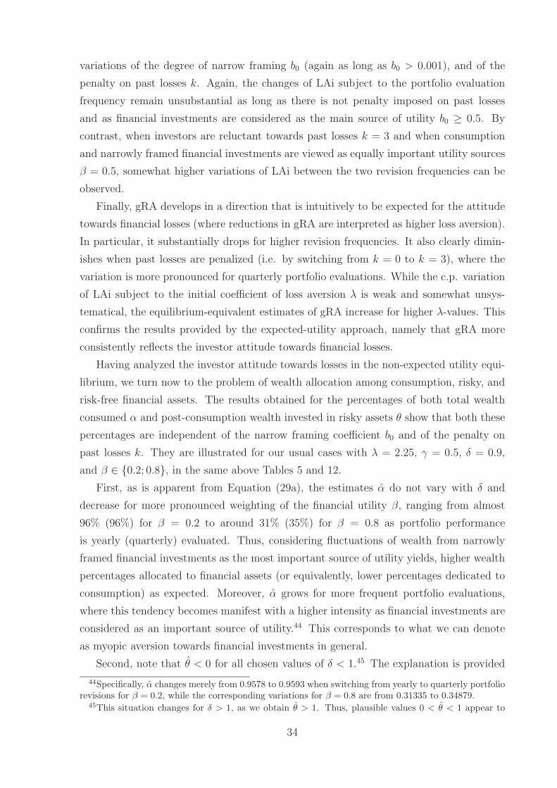
variations of the degree of narrow framing b0 (again as long as b0 > 0.001), and of the

penalty on past losses k. Again, the changes of LAi subject to the portfolio evaluation

frequency remain unsubstantial as long as there is not penalty imposed on past losses

and as financial investments are considered as the main source of utility b0 ≥ 0.5. By

contrast, when investors are reluctant towards past losses k = 3 and when consumption

and narrowly framed financial investments are viewed as equally important utility sources

β = 0.5, somewhat higher variations of LAi between the two revision frequencies can be

observed.

Finally, gRA develops in a direction that is intuitively to be expected for the attitude

towards financial losses (where reductions in gRA are interpreted as higher loss aversion).

In particular, it substantially drops for higher revision frequencies. It also clearly dimin-

ishes when past losses are penalized (i.e. by switching from k = 0 to k = 3), where the

variation is more pronounced for quarterly portfolio evaluations. While the c.p. variation

of LAi subject to the initial coefficient of loss aversion λ is weak and somewhat unsys-

tematical, the equilibrium-equivalent estimates of gRA increase for higher λ-values. This

confirms the results provided by the expected-utility approach, namely that gRA more

consistently reflects the investor attitude towards financial losses.

Having analyzed the investor attitude towards losses in the non-expected utility equi-

librium, we turn now to the problem of wealth allocation among consumption, risky, and

risk-free financial assets. The results obtained for the percentages of both total wealth

consumed α and post-consumption wealth invested in risky assets θ show that both these

percentages are independent of the narrow framing coefficient b0 and of the penalty on

past losses k. They are illustrated for our usual cases with λ = 2.25, γ = 0.5, δ = 0.9,

and β ∈ {0.2; 0.8}, in the same above Tables 5 and 12.

First, as is apparent from Equation (29a), the estimates α do not vary with δ and

decrease for more pronounced weighting of the financial utility β, ranging from almost

96% (96%) for β = 0.2 to around 31% (35%) for β = 0.8 as portfolio performance

is yearly (quarterly) evaluated. Thus, considering fluctuations of wealth from narrowly

framed financial investments as the most important source of utility yields, higher wealth

percentages allocated to financial assets (or equivalently, lower percentages dedicated to

consumption) as expected. Moreover, α grows for more frequent portfolio evaluations,

where this tendency becomes manifest with a higher intensity as financial investments are

considered as an important source of utility.44 This corresponds to what we can denote

as myopic aversion towards financial investments in general.

Second, note that θ < 0 for all chosen values of δ < 1.45 The explanation is provided

44Specifically, α changes merely from 0.9578 to 0.9593 when switching from yearly to quarterly portfoliorevisions for β = 0.2, while the corresponding variations for β = 0.8 are from 0.31335 to 0.34879.

45This situation changes for δ > 1, as we obtain θ > 1. Thus, plausible values 0 < θ < 1 appear to

34

by Equation (29b), where this denominator of the first-line expression is always negative.

In essence, this denominator expresses the trade-off between the revenues from risk-free

vs. risky investments46 and decreases as risky investments become more profitable. In

other words, the denominator of this equilibrium expression of θ reflects the profitability

of risky with respect to risk-free assets taken with contrary sign. Recall now that θ stands

for the percentages of post-consumption wealth put in risky assets, hence it is expected

to grow as risky assets become more profitable. Therefore, only the absolute values of θ

can be meaningfully interpreted, and the subsequent comments refer to |θ|.

As noted below Equations (29), higher β-values entail higher θ, hence lower |θ|. This

tendency is slightly counterbalanced but never dominated by an increase in δ. Also recall

that |θ| > 1 shows that investors borrow extra-money at the risk-free rate and invest it

in the risky portfolio, which is the case for β ≤ 0.5. Apparently, for lower coverage of

consumption from additional incomes (i.e. low β-values, see for example Tables 6 and 13),

agents make surprisingly large investments in risky assets, as they probably welcome the

higher chances of gaining more money offered by risky investments. Across all considered

(β, δ)-combinations, |θ| varies between 67 − 944% (68 − 1008%) for yearly (quarterly)

portfolio evaluations. Moreover, the estimates of θ taken in absolute value are generally

lower for more frequent portfolio evaluations. Note also that |θ| is higher compared to the

mean percentages of post-consumption wealth invested in risky assets in the expected-

utility setting.

β = 0.8 β = 0.2k = 0 k = 3 k = 0 k = 3

I/C 3.5459 3.5459 1.1609 1.1609

(1 − α)|θ| 0.46184 0.46184 0.08826 0.08826

Table 6: The estimated wealth allocation in the non-expected utility setting for yearlydata, λ = 2.25, γ = 0.5 and δ = 0.9.

Finally, as θ does not reflect how total wealth is split between risky and riskless assets,

it cannot tell us anything about the aversion to financial risks in a strict sense. Across all

considered parameter-configurations, multiplying 1− α by |θ| amounts to around 9−78%

(9 − 77%) for yearly (quarterly) portfolio evaluations. As expected, the highest values

are obtained for maximal additional incomes (i.e. due to the fact that narrowly framed

financial investments are considered the most important utility source β = 0.8 and/or

be possible only for 1 < δ < 2. However, δ > 1 yields implausible values for other model parameters inequilibrium. In addition, the corresponding estimates in the expected-utility setting are also implausible.For this reason, we do not further analyze cases with δ > 1.

46The denominator is close to the the expected equity premium taken with a negative sign, namely−(Et(Rt+1) − Rf ) ≃ Rf − exp(r + σ2

r/2). Specifically, the risky returns are amended according to theircorrelation to consumption.

35

that δ is minimal). For β = 0.8, over 46% (44%) of the total wealth is dedicated to risky

assets in equilibrium when portfolios are evaluated once a year (every three months). For

β = 0.2, the respective percentages are very similar for both revision frequencies and lie

below 9%. These results are captured in Tables 6 and 13 for δ = 0.9. Thus, we can

observe merely small changes in the percentages of total wealth invested in risky assets,

as investors evaluate their portfolios more frequently. These changes are more evident

for higher values of β. Based on this, we conclude that myopic loss aversion continues

to hold in the two-dimensional utility setting with non-expected utility, but only as long

as investors consider the utility derived form financial wealth fluctuations sufficiently

important relative to the consumption utility. Even in this case, the myopic loss aversion

holds in a softer form, as investors who evaluate their risky portfolios more often invest

only slightly lower proportions of their total wealth in risky assets. Thus, maximizing non-

expected utility appears to require in equilibrium a more relaxed attitude towards risky

investments compared to the situation when expected utility is maximized. Moreover,

relative to the findings in Rengifo and Trifan (2006) where financial investments are the

sole source of utility, investors who maximize two-dimensional utility are more (less) open

to risky investments, depending on whether narrowly framed financial investments are

perceived as the most (least) important utility source.47

As a final remark, we note that both equilibrium percentages of total wealth dedicated

to consumption α and of post-consumption wealth invested in risky assets θ are insensitive

to the choice of the initial λ. Consequently, the same holds for the percentages of total

wealth dedicated to risky assets (1 − α)|θ|.

3.4 A summary comparison of the two approaches: expected

and non-expected utility

We note that comparing the two considered settings with expected and non-expected

utility is not an easy task. In spite of the “preventive measures” adopted in order to

ensure the possibility of performing such comparisons (namely concerning the additional

income and the values of the behavioral parameters), they employ distinct estimation

procedures and hence deliver different parameter estimates. The former setting offers the

additional advantage of being less complex and more intuitive, while the latter one allows

us to directly estimate more variables of interest, especially those regarding the optimal

wealth allocation. In spite of the claim in Barberis, Huang, and Thaler (2003) that

non-expected utility better describes decision making under risk, it is difficult to reach

47In essence, the percentages of total wealth invested in risky assets in the one- and two-dimensionalutility settings lie closest to each other for the somewhat ambiguous situation with β = 0.5 and middle-range δ-s, in sum for middle-range additional incomes.

36

a clear-cut conclusion about the adequacy of one or another of the settings developed in

the present work, as they provide both common and specific results.

We start by noting the most important results that are similar under both approaches.

First, excessively high values of the consumption-related risk aversion coefficient γ are in-

compatible with the idea of aggregate equilibrium under both approaches. Also, the lack

of narrow framing of financial investments does not corroborate with the manifestation

of an attitude towards financial investments (in particular towards losses) and effectively

entails less plausible parameter estimates. Second, the aggregate markets where the repre-

sentative investor maximizes expected and non-expected utility require similar attitudes

towards financial losses. In particular, the loss aversion coefficient in equilibrium λ as

well as the other two measures of this attitude LAi and gRA reach values that are very

close to each other and exhibit similar evolutions subject to the variation of behavioral

model parameters in both settings. The sole difference refers to the variation of λ subject

to the revision frequency that appears to be dictated in the non-expected utility setting

by the importance ascribed to financial relative to consumption utility. Also, under both

approaches LAi closely follows λ and gRA appears to offer a more intuitive support of

how the attitude towards losses changes.

On the other hand, maximizing expected and non-expected utility entail different re-

sults with respect to the wealth allocation among consumption, risky, and risk-free finan-

cial assets. This can in part be due to the above mentioned discrepancies in methodology.

Specifically, in the expected-utility setting this wealth allocation can only be assessed on

average, on the basis of the equilibrium estimates of other variables. By contrast, the non-

expected utility approach prescribes exact values of the allocation variables in the market

equilibrium. In particular, our empirical results show that investors who maximize non-

expected utility appear to be substantially more reluctant towards financial investments

in general, but more open towards investing in risky assets. The respective fractions of

total wealth to be consumed in the aggregate equilibrium attain more plausible (namely

higher) values than under the expected-utility approach. The variation of the total-wealth

percentages invested in risky assets is more pronounced and their overall values higher.

Moreover, myopic loss aversion clearly holds under expected-utility maximization. Yet, it

becomes manifest in the non-expected utility framework only when investors consider the

financial utility sufficiently important relative to the consumption utility. Even in this

case, the wealth percentages dedicated to risky assets decrease only slightly for higher

evaluation frequencies. Finally, investors with an additional source of utility appear to

behave differently when maximizing expected utility or non-expected utility, with respect

to their peers who derive utility exclusively from financial investments. Thus, while max-

imizing expected two-dimensional utility renders them more circumspect towards risky

37

investments, maximizing non-expected two-dimensional utility yields the same only when

consumption utility is considered more important than financial one. Otherwise, investors

put substantially more money in risky assets relative to the one-sided utility approach.

4 Summary and conclusions

This paper extends the model in Rengifo and Trifan (2006) by analyzing loss attitude

and wealth allocation in a two-dimensional utility framework. Specifically, one question

we attempt to answer is how non-professional investors who derive utility from both con-

sumption and (narrowly framed) financial investments behave when faced with financial

risk. A related problem we tackle refers to how these investors consequently split their

money between consumption, and risky vs. risk-free financial assets.

Following Barberis, Huang, and Thaler (2003) and Barberis and Huang (2004a,b), we

consider two different ways of estimating prospective utility, namely either as expected or

as non-expected utility. In both situations, we explicitly account for the narrow framing of

financial investments, as well as for the impact of past performance on current perceptions.

In this broader setting, we derive the necessary conditions for equilibrium in the aggregate

market with a representative investor. Fixing general market parameters (such as the

dynamics of consumption and of the expected returns), and several behavioral parameters

specific to our model (such as the degree of narrow framing and the risk aversion to

consumption), these conditions provide a basis for the derivation of the prospective value

ascribed to risky investments in equilibrium. An equivalent loss aversion coefficient can

then be estimated from the definition of this prospective value. In addition, the expected-

utility setting allows for the estimation of the coefficient by which utility is discounted in

time. The byproducts of the estimation procedure in the non-expected utility setting are

the percentages of total wealth allocated to consumption and of post-consumption wealth

invested in risky assets.

The theoretical results are subsequently tested and extended in an empirical context.

We assess the equilibrium values and investigate the sensitivity of the variables of inter-

est for various configurations of the behavioral parameters and for two distinct portfolio

evaluation horizons (one year and three months). In order to avoid the impossibility of

covering current consumption needs from financial revenues throughout the entire invest-

ing period, we also consider that investors periodically dispose of exogenous additional

incomes. These incomes are shaped in order to ensure the equivalency of the two settings

with expected and non-expected utility. We also analyze the variation of the equilibrium

estimates with respect to changes in the magnitude of additional incomes.

The common and specific empirical findings under the two approaches with expected

38

and non-expected utility can be summarized as follows. First, in both settings we can

isolate equilibrium-incompatible parameter constellations. One the one hand, they are

characterized by too high values of the consumption-related risk aversion coefficient. On

the other hand, the lack of narrow framing entails implausible estimates in the expected-

utility setting and unusual ones (relative to the values obtained for the remaining cases) in

the non-expected utility framework. These cases are then discarded from the subsequent

analysis.

Second, the loss aversion coefficients are very close to each other and also close to the

“loss-neutral” value of 1 in both expected- and non-expected utility settings. Specifically,

they lie slightly above (below) 1 for yearly (quarterly) portfolio evaluations. Thus, the

coefficient of loss aversion required in order to attain the market equilibrium is clearly lower

than 2.25, the value suggested by the original prospect theory. This indicates that the

aversion towards financial losses is less pronounced when consumption is considered as an

additional source of utility besides financial wealth fluctuations. Other things being equal,

the loss aversion coefficients required to attain the aggregate equilibrium in both settings

grow subject to higher degrees of narrow framing and drop when investors penalize past

losses. Yet, in the expected-utility setting the same coefficient of loss aversion diminishes

for more frequent risky performance checks. By contrast, under non-expected utility the

corresponding variation is dictated by the importance ascribed to financial utility relative

to consumption utility (specifically, for a higher importance we can observe the same

reduction in the loss aversion coefficient for more frequent evaluations).

Furthermore, the other two measures of the investor attitude towards financial losses

employed evolve in equilibrium similarly to the estimated loss aversion coefficients. The

loss aversion index follows closely the simple loss aversion coefficient, being slightly lower.

The global first-order risk aversion appears to describe more consistently and more intu-

itively the actual attitude towards financial losses and its variations subject to changes in

the behavioral model parameters.

Third, the prospective value in equilibrium is always negative, suggesting that the

overall utility diminishes with financial investments. This decrease in utility substantially

shrinks as investors pay more attention to financial investments (i.e. by more intense

narrow framing), as this attention is coupled with a positive image of the opportunities

they might offer.

Fourth, the allocation of wealth between consumption and (risky and riskless) financial

assets can be explicitly determined in the non-expected utility setting, where the equi-

librium equations deliver the necessary estimates. Under the maximization of expected

utility, this optimal allocation can only be assessed on average.

In the expected-utility framework, investors appear to allocate modest percentages

39

of their total wealth to consumption, which also vary in high extent with the additional

income meant to cover current consumption needs. The respective values amount to be-

tween 2 − 21% (1 − 13%) for yearly (quarterly) portfolio evaluations, where the highest

ones are obtained for minimal additional incomes. These small values should be under-

stood in terms of our assumption that the total wealth includes the additional incomes,

which implies that it increases faster than the consumption subject to higher additional

incomes. By contrast, attaining the aggregate equilibrium when investors maximize non-

expected utility requires substantial allocations for consumption purposes. The respective

percentages yield 31−96% (35−96%) for yearly (quarterly) performance checks and vary

much less subject to the portfolio evaluation frequency. In neither of the two settings

does the fractions of total wealth dedicated to consumption vary either with the degree

of narrow framing or with the penalties imposed on past losses.

Moreover, in the expected-utility setting the percentages of post-consumption wealth

invested in risky assets increase as the additional income covers more than current con-

sumption needs (specifically, as it provides extra money to be invested in financial assets

after accounting for consumption). The respective overall values lie around 27 − 45%

(2 − 17%) for yearly (quarterly) portfolio evaluations. The non-expected equilibrium de-

livers corresponding estimates that have to be interpreted in absolute value. For lower

additional incomes, investors become very interested in risky assets, as they even borrow

extra money for the purpose of increasing the risky investment. The minimal proportions

of post-consumption wealth in the non-expected utility equilibrium lie above 67% (68%)

for yearly (quarterly) portfolio evaluations and often exceed 100%. In both settings, the

fractions of post-consumption wealth invested in risky assets are invariable with respect

to the degree of narrow framing, but they slightly diminish when past losses are penalized

in the expected-utility framework.

Finally, the resulting percentages of total wealth put in risky assets yield 22 − 43%

(2−17%) when expected utility is maximized and portfolio performance is evaluated yearly

(quarterly). These values remain below the values obtained in the one-dimensional utility

framework of Rengifo and Trifan (2006). The respective percentages in the non-expected

equilibrium vary much more subject to the magnitude of the additional income, but appear

to be less influenced by the changes in the evaluation frequency. Specifically, between

9− 78% (9− 77%) of total wealth is invested in risky assets by investors maximizing non-

expected utility. These values are hence higher (lower) than the average percentages which

result when investors derive utility merely from financial investments, as the additional

utility source, i.e. the consumption, becomes less (more) important.

In sum, these numbers support the idea that investors who check the performance

of their portfolios more frequently invest less money in risky assets. Thus, myopic loss

40

aversion continues to manifest when utility has twofold sources, albeit in a much softer

form and merely for sufficiently high additional incomes when non-expected utility is

maximized.

Fifth, our estimates appear to vary slightly and, as anticipated, proportionally with

the initial loss aversion coefficient. The sole exception is obtained under the non-expected

utility approach, where the loss aversion coefficient in equilibrium differently fluctuates

subject to the initial loss aversion, depending on the magnitude of the the additional

income. However, the corresponding variations remain low on average.

Concerning the expected-utility setting, the estimated discounting factor is found to

lie close to the values proposed in the literature. Furthermore, it does not vary with the

degree of narrow framing or the additional income, and is higher and less sensitive to

changes in the consumption-based risk-aversion when portfolios are evaluated more often.

In sum, maximizing expected and non-expected utility when financial investments are

narrowly framed reaches similar equilibrium results concerning the attitude to financial

losses. By contrast, the two settings offer different pictures concerning the wealth allo-

cation between consumption and risky and riskless assets in equilibrium. In particular,

investors maximizing expected-utility appear to dedicate on average surprisingly small

amounts of money to consumption and to behave on average myopically loss averse with

respect to risky investments. The non-expected approach sets clear-cut target values for

the wealth percentages to be consumed and invested in risky assets in order to reach

the aggregate equilibrium. Specifically, both these percentages are substantially higher,

but also less variable in the evaluation frequency than in the expected-utility setting.

Consequently, under the non-expected utility approach, the aversion towards financial

investments in general is more pronounced, but the attitude towards risky investments in

particular is more relaxed, and myopic loss aversion holds merely in soft form and only

when the financial wealth fluctuations are viewed as the major utility source.

41

5 Appendix

5.1 Descriptive statistics

SP500 10-year bond Consumption

Evaluation frequency

Quarterly Yearly Quarterly Yearly Quarterly YearlyMean 0.017 0.066 0.017 0.073 0.016 0.052

Median 0.018 0.071 0.017 0.070 0.001 0.049Std.Dev. 0.079 0.136 0.006 0.026 0.008 0.022Kurtosis 2.661 -0.9659 0.623 0.974 0.673 -1.084Skewness -0.671 -0.205 0.951 1.042 -0.018 0.165

Max. 0.290 0.345 0.036 0.142 0.042 0.090Min. -0.302 -0.207 0.009 0.037 -0.010 0.011Obs. 175 43 175 43 175 43

Table 7: Log-differences of the SP500 index and of the ten-year bond returns forquarterly and yearly portfolio evaluations.

5.2 The expected-utility approach

42

β = 0.8 β = 0.2γ = 0.5 γ = 1 γ = 0.5 γ = 1

k = 0 k = 3 k = 0 k = 3 k = 0 k = 3 k = 0 k = 3b0 = 5

ρ 0.99059 0.99059 0.99842 0.99842 0.99059 0.99059 0.99842 0.99842

V -45.961 -45.961 -6,162.7 -6,162.7 -45.96085 -45.96085 -6,162.69240 -6,162.69240

λ 1.0104 1.0085 2.3751 2.3772 0.99221 0.99021 1.54749 1.54707b0 = 10

ρ 0.99059 0.99059 0.99842 0.99842 0.99059 0.99059 0.99842 0.99842

V -22.98 -22.98 -3,081.3 -3,081.3 -22.98042 -22.98042 -3,081.34620 -3,081.34620

λ 1.0033 1.0014 1.6863 1.6863 0.99085 0.98883 1.26964 1.26840b0 = 100

ρ 0.99059 0.99059 0.99842 0.99842 0.99059 0.99059 0.99842 0.99842

V -2.298 -2.298 -308.13 -308.13 -2.29804 -2.29804 -308.13462 -308.13462

λ 0.99698 0.99505 1.0663 1.0646 0.98962 0.98758 1.0196 1.0176b0 = 1, 000

ρ 0.99059 0.99059 0.99842 0.99842 0.99059 0.99059 0.99842 0.99842

V -0.2298 -0.2298 -30.813 -30.813 -0.22980 -0.22980 -30.81346 -30.81346

λ 0.99634 0.99441 1.0043 1.0024 0.98950 0.98746 0.99458 0.99252

Table 8: The main estimated parameters in the expected-utility setting for quarterly data, λ = 2.25 and δ = 0.9.

43

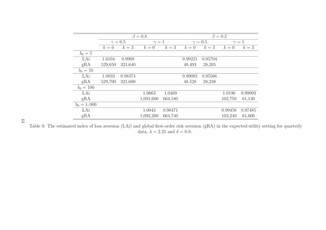
β = 0.8 β = 0.2γ = 0.5 γ = 1 γ = 0.5 γ = 1

k = 0 k = 3 k = 0 k = 3 k = 0 k = 3 k = 0 k = 3b0 = 5LAi 1.0104 0.9908 2.3751 2.3595 0.99221 0.95704 1.5475 1.5294gRA 529,650 321,640 1,079,100 652,240 48,493 28,205 92,229 51,205

b0 = 10LAi 1.0033 0.98374 1.6863 1.6687 0.99085 0.95566 1.2696 1.2507gRA 529,700 321,690 1,085,700 658,520 48,528 28,238 97,764 56,429

b0 = 100LAi 0.99698 0.97738 1.0663 1.0469 0.98962 0.95441 1.0196 0.99993gRA 529,740 321,730 1,091,600 664,180 48,560 28,268 102,750 61,130

b0 = 1, 000LAi 0.99634 0.97674 1.0043 0.98471 0.9895 0.95429 0.99458 0.97485gRA 529,740 321,740 1,092,200 664,740 48,563 28,272 103,240 61,600

Table 9: The estimated index of loss aversion (LAi) and global first-order risk aversion (gRA) in the expected-utility setting for quarterlydata, λ = 2.25 and δ = 0.9.

44

β = 0.8 β = 0.2γ = 0.5 γ = 1 γ = 0.5 γ = 1

k = 0 k = 3 k = 0 k = 3 k = 0 k = 3 k = 0 k = 3

C/W 0.01866 0.01866 0.00975 0.00975 0.12545 0.12537 0.07108 0.07105

I/C 3.1856 3.1856 5.5556 5.5556 1.1583 1.1583 1.3889 1.3889

θ 0.15451 0.14439 0.1633 0.15316 0.03233 0.02182 0.09719 0.08692

(1 − C/W )θ 0.15163 0.14170 0.16171 0.15167 0.02827 0.01908 0.09028 0.08074

Table 10: The estimated wealth allocation in the expected-utility setting for yearly data,λ = 2.25 and δ = 0.9.

5.3 The non-expected utility approach

45

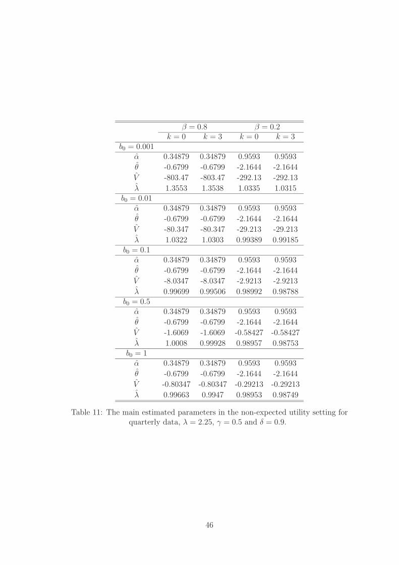
β = 0.8 β = 0.2k = 0 k = 3 k = 0 k = 3

b0 = 0.001α 0.34879 0.34879 0.9593 0.9593

θ -0.6799 -0.6799 -2.1644 -2.1644

V -803.47 -803.47 -292.13 -292.13

λ 1.3553 1.3538 1.0335 1.0315b0 = 0.01

α 0.34879 0.34879 0.9593 0.9593

θ -0.6799 -0.6799 -2.1644 -2.1644

V -80.347 -80.347 -29.213 -29.213

λ 1.0322 1.0303 0.99389 0.99185b0 = 0.1

α 0.34879 0.34879 0.9593 0.9593

θ -0.6799 -0.6799 -2.1644 -2.1644

V -8.0347 -8.0347 -2.9213 -2.9213

λ 0.99699 0.99506 0.98992 0.98788b0 = 0.5

α 0.34879 0.34879 0.9593 0.9593

θ -0.6799 -0.6799 -2.1644 -2.1644

V -1.6069 -1.6069 -0.58427 -0.58427

λ 1.0008 0.99928 0.98957 0.98753b0 = 1

α 0.34879 0.34879 0.9593 0.9593

θ -0.6799 -0.6799 -2.1644 -2.1644

V -0.80347 -0.80347 -0.29213 -0.29213

λ 0.99663 0.9947 0.98953 0.98749

Table 11: The main estimated parameters in the non-expected utility setting forquarterly data, λ = 2.25, γ = 0.5 and δ = 0.9.

46

β = 0.8 β = 0.2k = 0 k = 3 k = 0 k = 3

b0 = 0.001LAi 1.3553 1.3361 1.0335 0.9983gRA 528,060 320,079 48,151 27,871

b0 = 0.01LAi 1.0322 1.0126 0.99389 0.95868gRA 529,580 321,570 48,522 28,232

b0 = 0.1LAi 0.99986 0.98027 0.98992 0.95472gRA 529,730 321,720 48,559 28,268

b0 = 0.5LAi 0.99699 0.97739 0.98957 0.95436gRA 529,740 321,730 48,562 28,271

b0 = 1LAi 0.99663 0.97703 0.98953 0.95432gRA 529,740 321,730 48,563 28,271

Table 12: The estimated index of loss aversion (LAi) and global first-order risk aversion(gRA) in the expected-utility setting for quarterly data, λ = 2.25, γ = 0.5 and δ = 0.9.

β = 0.8 β = 0.2k = 0 k = 3 k = 0 k = 3

I/C 3.1856 3.1856 1.1583 1.1583

(1 − α)|θ| 0.44276 0.44276 0.08809 0.08809

Table 13: The estimated wealth allocation in the non-expected utility setting for yearlydata, λ = 2.25, γ = 0.5 and δ = 0.9.

47

References

Barberis, N., and M. Huang (2004a): “The Loss Aversion/Narrow Framing Approach

to Stock Market Pricing and Participation Puzzles,” Working paper, University of

Chicago, Stanford University.

(2004b): “Preferences with Frames: A New Utility Specification that Allows for

the Framing of Risks,” Working paper, University of Chicago, Stanford University.

Barberis, N., M. Huang, and T. Santos (2001): “Prospect Theory and Asset

Prices,” Quarterly Journal of Economics, 116, 1–53.

Barberis, N., M. Huang, and R. Thaler (2003): “Individual Preferences, Monetary

Gambles and the Equity Premium,” Working paper, University of Chicago, Stanford

University.

Campbell, R., R. Huisman, and K. Koedijk (2001): “Optimal Portfolio Selection

in a Value-at-Risk Framework,” Journal of Banking and Finance, 25, 1789–1804.

Kobberling, V., and P. Wakker (2005): “An Index of Loss Aversion,” Journal of

Economic Theory, 122, 119–131.

Rengifo, E., and E. Trifan (2006): “Investors Facing Risk: Loss Aversion and Wealth

Allocation Between Risky and Risk-Free Assets,” Working paper, Darmstadt Uni-

versity of Technology.

48