Danish Meteorological Institute - DMI · Danish Meteorological Institute Scientiﬁc Report 12-03...

Danish Meteorological InstituteMinistry for Climate and Energy

Copenhagen 2012www.dmi.dk/dmi/sr12-03.pdf page 1 of 21

Scientific Report 12-03

Mixing in HBM

Per Berg

Danish Meteorological InstituteScientific Report 12-03

ColophoneSerial title:Scientific Report 12-03

Title:Mixing in HBM

Subtitle:

Authors:Per Berg

Other Contributers:

Responsible Institution:Danish Meteorological Institute

Language:English

Keywords:mixing, structure functions, k-ω turbulence model, third order moments, convection, buoyancyproduction, vertical diffusivity, surface roughness length scale, critical gradient Richardson number,Neumann boundary conditions, HBM model

Url:www.dmi.dk/dmi/sr12-03.pdf

ISSN:

ISBN:978-87-7478-610-8

Version:1.0

Website:www.dmi.dk

Copyright:Danish Meteorological Institute

www.dmi.dk/dmi/sr12-03.pdf page 2 of 21


ContentsColophone . . . . . . . . . . . . . . . . . . . . . . . . . . . . . . . . . . . . . . . . . 2

Preface 4Front Page 4

1 Introduction 52 Summary 53 Structure Functions And Vertical Diffusivities 64 The k-ω Model Equations 85 Determine Coefficients In Two-Equation Turbulence Models 96 Parameterization of Breaking Internal Waves 127 Parameterization of Breaking Surface Waves 128 Boundary Conditions 139 Extended Buoyancy Production During Convection 1410 Thermal Diffusivity 1511 Penetrating Insolation 1512 Discretization And Solution Method 1613 Concluding Remarks 16

References 17Previous reports 18Appendix 1: Constants In The Structure Functions 18Appendix 2: Critical Value Of The Gradient Richardson Number 18Appendix 3: Computation Of The Structure Functions 20



PrefaceThe mixing scheme as described here is implemented into the HIROMB-BOOS ocean circulationmodel, HBM (Berg and Poulsen, 2012), and has proved its worth for some years in operationalapplications such as the DMI storm surge forecast model and in the MyOcean Baltic model.

The present document is the proper choice if you need a reference to the mixing scheme in HBM. Itis appreciated if you quote the present document as well as the general implementation document forthe HBM model by Berg and Poulsen (2012).

Front PageThe figures on the front page shows modelled profiles of salinity and temperature at four stationsduring 2007:From top to bottom BMP13 in Botnian Bay, Læsø Øst in Kattegat, BMPK2 in Bornholm Basin andBMPI2 in Gotland Deep; salinity to the left and temperature to the right; vertical axis is depth andhorizontal axis is time.

These results are obtained by the MyOcean Baltic V2 set-up using the latest release of the HBMcode. Plotting of the results was made by Priidik Lagemaar and Germo Väli (Marine SystemsInstitute, Tallinn University of Technology) for the "Scientific Calibration Report (ScCR) for V2,WP 6 - Baltic MFC" of the MyOcean project, reference: MYO-WP6-ScCR-V2.



1. IntroductionA good turbulence model has extensive universality, and is not too complex to develop or use. Uni-versality implies that a single set of empirical constants or functions, inserted into the equations,provides close simulation of a large variety of types of flow. Complexity is measured by the number ofdifferential equations which the model contains, and the number of empirical constants and functionswhich are required to complete them; increase in the first complicates the task of using the model,increase in the second that of developing it.

LAUNDER AND SPALDING, 1973.

In ocean circulation models of the type considered here one solves equations for the mean variables.Mixing, which enters through non-resolved, higher-order moments of the fluctuating components ofthe variables, can be expressed in terms of vertical diffusivities and vertical gradients of the resolvedmean variables. The reliability of a mixing scheme - which is the model of providing the verticaldiffusivities - is predicated upon the physical content of its ingredients, and it is these ingredientswhich we have attempted to improve from previous models.

Our new mixing scheme consists of a two-equation turbulence closure model and algebraic structurefunctions. The two-equation turbulence closure model consists of transport equations for theturbulent kinetic energy, k, and for the inverse turbulent time scale or turbulent frequency, ω. Thestructure functions are algebraic functions not only of the gradient Richardson number as is mostoften the case, but also of the gradients of temperature and salinity and of the turbulent time scale.These choices are motivated by the need for properties such as accuracy, robustness, physicalsoundness, general applicability, and flexibility to add new features, still maintaining an acceptablelevel of the computational costs. Thus, from our own experience and testing as well as fromliterature, e.g. (Umlauf et al., 2003), the k-ω turbulence model has convincingly proved superior toother two-equation models, i.e. better than or at least as good at the same computational cost, and thestructure functions of (Canuto et al., 2002) follow a formalism sufficiently general to describe theneeded range of processes and to allow for extensions (plug-in features), yet not being toocumbersome to maintain.

Using well-known procedures, it then becomes a matter of algebra, rather than physics or empiricalreasoning, to derive expressions for the vertical diffusivities in terms of the prognostic variables ofthe two-equation turbulence model and gradients of the resolved mean variables of the circulationmodel.

2. SummaryOur scheme is based on the - in aerodynamics - classical k-ω turbulence model (Wilcox, 1988)extended for buoyancy affected geophysical flows by Umlauf et al. (2003) but we apply a new set ofcoefficients developed by the present author to obtain consistency during transition between thedifferent regimes of turbulence being predicted by the model. Through parameterizations we takeboth breaking surface waves (Craig and Banner, 1994) and internal waves (Axell, 2002) into accountin the turbulence model. The atmospheric forcing (i.e. wind stress and cooling surface heat flux) ofthe turbulence model is provided through a new set of surface flux boundary conditions for k and forω . We have introduced a new way of parameterizing extended buoyancy production during



convection into the turbulence model, by inclusion of third order moments using concepts from(Abdella and McFarlane, 1997; D’Alessio et al., 1998).

Different algebraic structure functions are applied for the vertical diffusivities of momentum, heatand salt. We have reconstructed the structure functions of (Canuto et al., 2002) into new,computationally sound expressions in turbulent time scale, temperature gradient, salinity gradient,resolved velocity shear and unresolved but parameterized shear from breaking internal waves.

To account for penetration of short wave radiation into the subsurface model layers aparameterization of the insolation properly suited for the Baltic Sea area was implemented (Meier,2001).

Also, during storm cases, to avoid the surface flow from increasing to unrealistically high currentspeeds, our implementation of the wind stress uses the effective wind velocity relative to the currentvelocity. A realistic description of the surface roughness length scale as seen from the ocean, z0, isone of the major unsolved problems is oceanography, and our choice of implementing z0 as beingproportional to the turbulent surface velocity scale comes from considerable numericalexperimentation in attempt to obtain good predictions in storm cases, both with respect to high waterand to low water situations. During calm situations a constant z0 of 10 cm is sufficient. It is, however,of vital importance that there is consistency between the z0 applied in the turbulence model and thez0 applied in the momentum equations, otherwise it may lead to spurious results in the forecasts.

An overview of our complete mixing scheme with some details is given in the following sections.First, in section 3, we describe the structure functions and the vertical diffusivities. Obtaining thevertical diffusivities is what is needed for obtaining closure to the system; the remaining sections ofthis document thus deal with determining the terms from which we can construct the verticaldiffusivities. In section 4, we state the k-ω model equations. Then, in section 5, we describe theprocedure for determining the coefficients of two-equation turbulence models consistently with thechosen stability functions and the physics being predicted. Parameterization of breaking internalwaves and surface waves is described in section 6 and 7, respectively. Our new formulation of the setof surface boundary conditions for the k-ω turbulence model is given in section 8. Section 9describes how we parameterize convection from third order moments. Thermal diffusivity andinsolation is briefly described in section 10 and 11, respectively, before we end with a shortdescription of how we have implemented the mixing scheme.

Most of the sometimes rather lengthy derivations and equations are left out of this document,though. It must be emphasised that our new mixing scheme has not yet been published and thepresent report documents original work by the author. More detailed documentation and validationexists as internal and personal notes at DMI, extracts of which constitute the present document.

3. Structure Functions And Vertical DiffusivitiesTo bring closure to the system of equations in our ocean circulation model we need to determine thethree vertical diffusivities, namely KM for momentum, KH for heat, and KS for salinity. These canbe expressed as

Ki = 2k2

εSi with i = M,H or S

where k is the turbulent kinetic energy and ε is the dissipation rate of turbulent kinetic energy. Thedimensionless functions Si are called structure (or sometimes, stability) functions. For constructingsuitable structure functions there is a variety of approaches described in the literature as well as



implemented in ocean circulation models worldwide, ranging from simple constants to moreinvolved expressions, including a variety of different features. A comparative analysis of somecandidate formulations is given in (Burchard and Bolding, 2001). We have, however, chosen themore recent structure functions of Canuto et al. (2002) which, despite relatively high complexity,after some algebra with pen and paper turned out to become usable for operational oceanographicapplications. In brief, these structure functions are expressed in terms of gradients of the prognosticvariables of the ocean circulation model and of the turbulent time scale. We have also introduced’shear’ of unresolved scales (i.e. from parameterized internal wave breaking) into the formulae.

Below we give a brief description of the structure functions, but before that we need to define somebasic quantities. The gradients of the mean salinity and temperature enter through RS and RH whichare given by

RS = gβS∂S

∂z

RH = gαH∂θ

∂z

in which S is salinity, θ is temperaure, z is the vertical coordinate with positive direction upwards, gis gravity, βS is the local haline contraction coefficient and αH is the local thermal expansioncoefficient. The density gradient enters through the buoyancy frequency squared

N2 = −gρ

∂ρ

∂z= RH −RS

The total shearΣ2T = Σ2 + σ2

is contributed by the resolved, large scale shear of the mean flow

Σ2 =

(∂u

∂z

)2

+

(∂v

∂z

)2

where (u, v) is the mean current, and by unresolved small scales which we for convenience haveadded up in the term σ. Such unresolved processes include e.g. internal wave breaking as discussedin section 6. The gradient Richardson number is defined as

Ri =N2

Σ2T

The first thing to do is then defining a critical value of the gradient Richardson number Ri,crit abovewhich turbulent mixing ceases to exist. In the regime Ri > Ri,crit we set Ki to a small backgroundvalue. A method to obtain Ri,crit as a function of the above-mentioned gradients was presented byCanuto et al. (2002). We have adapted their idea and from that we have constructed acomputationally sound procedure. Instead of going into algebraic details which involves treatingremovable singularities when RS and/or RH approaches zero, we jump directly to showing ourFortran 90 source code implementation in Appendix 2.

With Ri,crit in place, we can derive expressions for the structure functions Si which are valid in theregime Ri < Ri,crit. Again we lean towards the work of Canuto et al. (2002) and write eachstructure function as a fraction with a common denominator

Si =Ni

D



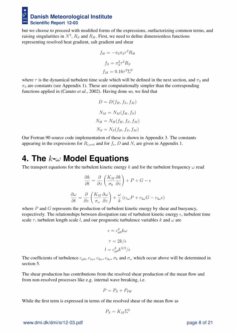
but we choose to proceed with modified forms of the expressions, outfactorizing common terms, andraising singularities in N2, RS and RH . First, we need to define dimensionless functionsrepresenting resolved heat gradient, salt gradient and shear

fH = −π2π3τ2RH

fS = π23τ

2RS

fM = 0.16τ 2Σ2

where τ is the dynamical turbulent time scale which will be defined in the next section, and π2 andπ3 are constants (see Appendix 1). These are computationally simpler than the correspondingfunctions applied in (Canuto et al., 2002). Having done so, we find that

D = D(fH , fS, fM)

NM = NM(fH , fS)

NH = NH(fH , fS, fM)

NS = NS(fH , fS, fM)

Our Fortran 90 source code implementation of these is shown in Appendix 3. The constantsappearing in the expressions for Ri,crit and for fi, D and Ni are given in Appendix 1.

4. The k-ω Model EquationsThe transport equations for the turbulent kinetic energy k and for the turbulent frequency ω read

∂k

∂t=

∂

∂z

(KM

σk

∂k

∂z

)+ P +G− ε

∂ω

∂t=

∂

∂z

(KM

σω

∂ω

∂z

)+ω

k(c1ωP + c2ωG− c3ωε)

where P and G represents the production of turbulent kinetic energy by shear and buoyancy,respectively. The relationships between dissipation rate of turbulent kinetic energy ε, turbulent timescale τ , turbulent length scale l, and our prognostic turbulence variables k and ω are

ε = c4µ0kω

τ = 2k/ε

l = c3µ0k3/2/ε

The coefficients of turbulence cµ0, c1ω, c2ω, c3ω, σk and σω which occur above will be determined insection 5.

The shear production has contributions from the resolved shear production of the mean flow andfrom non-resolved processes like e.g. internal wave breaking, i.e.

P = PS + PIW

While the first term is expressed in terms of the resolved shear of the mean flow as

PS = KMΣ2



the PIW term must be parameterized, see section 6. One might also consider adding aparameterization of shear production due to Langmuir circulation as done e.g. by Axell (2002); thishas also been implemented into the HBM code but it has not been used for any real production runyet.

The buoyancy production has contributions from gradients of the mean salinity and temperaturefields, and from higher order moments

G = KSRS −KHRH +GTOM

The last term GTOM is short-hand notation for our new way of parameterizing extended buoyancyproduction during convection by inclusion of third order moments (TOM) as will be described laterin section 9.

5. Determine Coefficients In Two-EquationTurbulence ModelsWe will determine the constants used in the mixing scheme to be consistent with the chosen structurefunctions and the physics being predicted. The procedure is new and might prove generallyapplicable to two-equation turbulence closure models, but it is here demonstrated only for the k-ωturbulence model. In the seven steps outlined below we will bring forward our argumentation for thechoice of closure coefficients.

Step 1: Having chosen an appropriate set of structure functions we need to determine the structureconstant cµ0. This is done by considering the structure function for momentum duringquasi-equilibrium when production equals dissipation, in the absence of buoyancy. After somealgebraic manipulations we find to four decimals precision that

cµ0 = 0.5234

Our value differs slightly from values found in the literature, where most studies depart from theclassical value cµ0 = 0.091/4 ≈ 0.5477, see e.g. (Launder and Spalding, 1974; Rodi, 1987; Wilcox,1988). An example is in (Umlauf et al., 2003) where cµ0 = 0.55, the rounded classical value, is used.The value cµ0 = 0.5562 is used by Burchard and Petersen (1999), by Axell and Liungman (2001) andby Axell (2002) without further argumentation. Other authors derive - like we do - a value of cµ0

consistently from the applied structure functions, e.g. cµ0 = 0.0771/4 ≈ 0.5268 was derived byBurchard and Bolding (2001) and is in very close agreement with our value due to the closerelationship between the applied structure functions (Canuto et al., 2001).

Step 2: While much literature on turbulence modelling, including (Burchard and Bolding, 2001;Meier, 2001; Axell, 2002), uses the value 0.4 for von Karman’s constant, κ, experiments and theorysuggest a range of values gathered around a slightly greater value, see e.g. (Long et al., 1993; Orszagand Patera, 1981). We here choose the representative value

κ = 0.41

Step 3: From grid-stirring experiments it is known that turbulence decays with distance according toa power law, see e.g. a summary in (Umlauf et al., 2003). That is, the geometric length scale, l,which is the turbulent length scale in the limit of neutral shear flow, has a linear variation

l = L(z0 − z) with 0.06 < L < 0.33 < κ



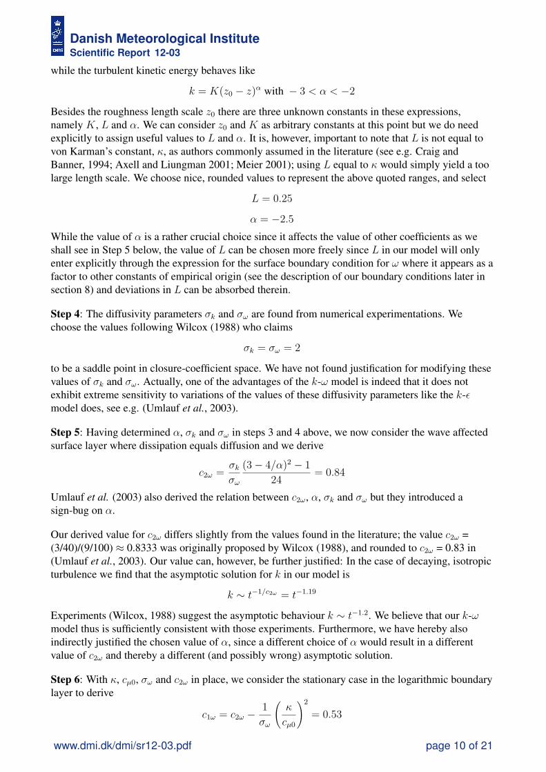
while the turbulent kinetic energy behaves like

k = K(z0 − z)α with − 3 < α < −2

Besides the roughness length scale z0 there are three unknown constants in these expressions,namely K, L and α. We can consider z0 and K as arbitrary constants at this point but we do needexplicitly to assign useful values to L and α. It is, however, important to note that L is not equal tovon Karman’s constant, κ, as authors commonly assumed in the literature (see e.g. Craig andBanner, 1994; Axell and Liungman 2001; Meier 2001); using L equal to κ would simply yield a toolarge length scale. We choose nice, rounded values to represent the above quoted ranges, and select

L = 0.25

α = −2.5

While the value of α is a rather crucial choice since it affects the value of other coefficients as weshall see in Step 5 below, the value of L can be chosen more freely since L in our model will onlyenter explicitly through the expression for the surface boundary condition for ω where it appears as afactor to other constants of empirical origin (see the description of our boundary conditions later insection 8) and deviations in L can be absorbed therein.

Step 4: The diffusivity parameters σk and σω are found from numerical experimentations. Wechoose the values following Wilcox (1988) who claims

σk = σω = 2

to be a saddle point in closure-coefficient space. We have not found justification for modifying thesevalues of σk and σω. Actually, one of the advantages of the k-ω model is indeed that it does notexhibit extreme sensitivity to variations of the values of these diffusivity parameters like the k-εmodel does, see e.g. (Umlauf et al., 2003).

Step 5: Having determined α, σk and σω in steps 3 and 4 above, we now consider the wave affectedsurface layer where dissipation equals diffusion and we derive

c2ω =σkσω

(3− 4/α)2 − 1

24= 0.84

Umlauf et al. (2003) also derived the relation between c2ω, α, σk and σω but they introduced asign-bug on α.

Our derived value for c2ω differs slightly from the values found in the literature; the value c2ω =(3/40)/(9/100) ≈ 0.8333 was originally proposed by Wilcox (1988), and rounded to c2ω = 0.83 in(Umlauf et al., 2003). Our value can, however, be further justified: In the case of decaying, isotropicturbulence we find that the asymptotic solution for k in our model is

k ∼ t−1/c2ω = t−1.19

Experiments (Wilcox, 1988) suggest the asymptotic behaviour k ∼ t−1.2. We believe that our k-ωmodel thus is sufficiently consistent with those experiments. Furthermore, we have hereby alsoindirectly justified the chosen value of α, since a different choice of α would result in a differentvalue of c2ω and thereby a different (and possibly wrong) asymptotic solution.

Step 6: With κ, cµ0, σω and c2ω in place, we consider the stationary case in the logarithmic boundarylayer to derive

c1ω = c2ω −1

σω

(κ

cµ0

)2

= 0.53



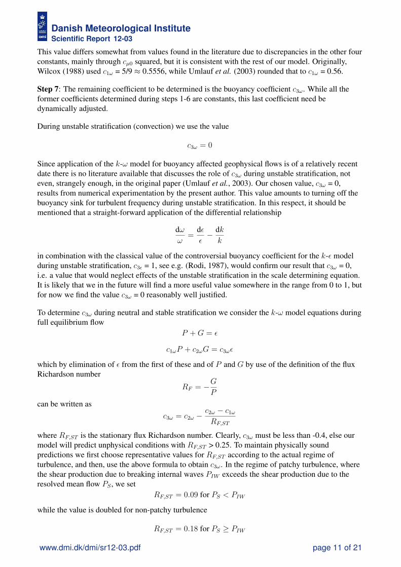
This value differs somewhat from values found in the literature due to discrepancies in the other fourconstants, mainly through cµ0 squared, but it is consistent with the rest of our model. Originally,Wilcox (1988) used c1ω = 5/9 ≈ 0.5556, while Umlauf et al. (2003) rounded that to c1ω = 0.56.

Step 7: The remaining coefficient to be determined is the buoyancy coefficient c3ω. While all theformer coefficients determined during steps 1-6 are constants, this last coefficient need bedynamically adjusted.

During unstable stratification (convection) we use the value

c3ω = 0

Since application of the k-ω model for buoyancy affected geophysical flows is of a relatively recentdate there is no literature available that discusses the role of c3ω during unstable stratification, noteven, strangely enough, in the original paper (Umlauf et al., 2003). Our chosen value, c3ω = 0,results from numerical experimentation by the present author. This value amounts to turning off thebuoyancy sink for turbulent frequency during unstable stratification. In this respect, it should bementioned that a straight-forward application of the differential relationship

dωω

=dεε− dk

k

in combination with the classical value of the controversial buoyancy coefficient for the k-ε modelduring unstable stratification, c3ε = 1, see e.g. (Rodi, 1987), would confirm our result that c3ω = 0,i.e. a value that would neglect effects of the unstable stratification in the scale determining equation.It is likely that we in the future will find a more useful value somewhere in the range from 0 to 1, butfor now we find the value c3ω = 0 reasonably well justified.

To determine c3ω during neutral and stable stratification we consider the k-ω model equations duringfull equilibrium flow

P +G = ε

c1ωP + c2ωG = c3ωε

which by elimination of ε from the first of these and of P and G by use of the definition of the fluxRichardson number

RF = −GP

can be written asc3ω = c2ω −

c2ω − c1ωRF,ST

where RF,ST is the stationary flux Richardson number. Clearly, c3ω must be less than -0.4, else ourmodel will predict unphysical conditions with RF,ST > 0.25. To maintain physically soundpredictions we first choose representative values for RF,ST according to the actual regime ofturbulence, and then, use the above formula to obtain c3ω. In the regime of patchy turbulence, wherethe shear production due to breaking internal waves PIW exceeds the shear production due to theresolved mean flow PS , we set

RF,ST = 0.09 for PS < PIW

while the value is doubled for non-patchy turbulence

RF,ST = 0.18 for PS ≥ PIW



These values for RF,ST are in close agreement with those used by Axell (2002). We are now able todetermine c3ω during neutral and stable stratification as

c3ω = −2.60 for PS < PIW

c3ω = −0.88 for PS ≥ PIW

This is a new approach to obtaining useful values for c3ω.

It should be noted, that Umlauf et al. (2003) occasionally obtain c3ω values which imply theunphysical condition RF,ST > 0.25, in their investigations of two-equation turbulence models andstructure functions.

6. Parameterization of Breaking Internal WavesDifferent approaches have been suggested for mixing below the mixed-layer in ocean circulationmodels, ranging from using simple constant background diffusivities to more complexparameterizations of internal waves, see e.g. (Canuto et al., 2002) for a summary. Here, we apply thework of Axell (2002) and let the shear production due to breaking internal waves during stablestratification have the following vertical distribution

PIW (z) =F0N(z)

ρ0Nave

with F0 = 0.9 mW/m2

where Nave is the depth averaged buoyancy frequency. The justification of this can be found fromthe numerical experiments performed by Axell (2002) who applies this production term to simulatedeep water mixing in the Baltic Sea.

7. Parameterization of Breaking Surface WavesThe wind drag is described in the usual way through

uF =√|τw| /ρ

τw = CDρair |W − u| (W − u)

where uF is the surface friction velocity and bold face letters indicate vector quantities, windvelocityW , current velocity u, and surface wind stress τw. The wind-strength dependent dragcoefficient CD will not be described further here.

There is little known about the surface roughness length scale z0 as seen from the ocean. Somemodels/authors apply a constant value of typically 10 cm or an approach à la Charnock

z0 ∝ HS = bSu2F

g

relating z0 to the significant wave height HS , i.e. relating the surface roughness length scale as seenfrom the atmosphere to the friction velocity squared through a free parameter bS . However, we findthe quadratic dependency too strong for high wind speeds and too mild for low wind speeds(remember, we must use the same z0 in the momentum equations). Numerical experimentationssuggest a linear relation to uF in absence of surface cooling and we are thus lead to choose

z0 =1

2

√ρ(q3)1/3



q3 = u3F + 0.54w3

H

The combined velocity scale q is thus expressed in terms of uF which is generated mechanically bythe wind, and of wH which is thermally produced by surface cooling. The convective velocity scalewH can physically be thought of as a sinking velocity of a parcel of fluid undergoing unstablesurface forcing through a negative surface buoyancy flux B, i.e.

wH = (−BH)1/3

where H is the mixed-layer depth, see later in section 9. The weight factor 0.54 is from (Fischer etal., 1979). In the absence of surface buoyancy (i.e. when B = 0) we see that z0 varies approximatelylinearly with the wind speed in our approach, which is different from what we see in most othermodels where z0 is chosen simply as a constant, or sometimes has the quadratic Charnock-likevariation.

8. Boundary ConditionsSome authors have suggested

KM

σk

∂k

∂z= mFu

3F −Bκz0 at z = 0

where the first term on the right hand side models the injection of turbulent kinetic energy due tosurface wave breaking, and mF=100 is an empirical constant suggested by Craig and Banner (1994)and later commonly used by modellers, see e.g. (Burchard, 2001; Meier, 2001; Umlauf et al., 2003).In the last term on the right hand side B is the negative surface buoyancy flux and κz0 is taken as ameasure of the surface roughness (Meier, 2001; Axell and Liungman, 2001).

Indeed, we agree with above mentioned authors that Neumann boundary conditions are superior toDirichlet boundary conditions for this purpose. However, we do not find it justified that κ shouldplay any role here since we are not likely dealing with a logarithmic boundary layer, see also thediscussion in (Umlauf et al., 2003). We find it much more plausible to apply the combined velocityscale q which was defined in the previous section. Thus, our new surface boundary condition for ksimply reads

KM

σk

∂k

∂z= mF q

3 at z = 0

We then derive the surface boundary conditions for ω analytically. From the power law of decay of kfrom the surface and the linear increase in length scale l, as we also used in step 3 of section 5, wedifferentiate with respect to z and apply the above-shown boundary condition for k at z=0. Aftersome algebra our new surface boundary condition for ω then becomes

KM

σω

∂ω

∂z=

1− 12α

σωLz0

(σk

−αLcµ0

mF q3

)2/3

at z = 0

The boundary conditions at the bottom are obtained by assuming, between the sea bottom and thelower-most grid point, a logarithmic boundary layer and a local balance between production anddissipation of turbulent kinetic energy, in the absence of buoyancy, and are commonly expressed interms of k and ε as

k =

(uFbcµ0

)2

ε =u3Fb

κz0b



where z0b is the bottom roughness length scale which we assign the typical value of 10 cm, and uFbis the friction velocity obtained from the bottom-most velocity components as

uF =√r (u2 + v2)

In the above, r is a model setup specific bottom roughness parameter with a typical value of around0.002. This formulation is unfortunately sensitive to the vertical grid resolution and there is noconsistency between the applied turbulence model and the bottom friction implemented in themomentum equations, which in some situations lead to some spurious model effects. A moreconsistent formualtion, in line with the above-shown approach for the surface boundary conditions,is under considerations/development.

9. Extended Buoyancy Production DuringConvectionThe only term we still need to find is GTOM which enters the buoyancy production, see section 4.We apply the usual notation with a prime denoting fluctuations, and angled brackets mean averagingover the grid cell and the time step of the circulation model. The buoyancy production may then beexpressed as a buoyancy flux which again is described in terms of a heat flux and a salinity flux

G = 〈b′w′〉 = g (αH〈θ′w′〉 − βS〈S ′w′〉)

The two flux terms are treated separately. After some manipulations of expressions derived in(D’Alessio et al., 1998), we arrive at

〈θ′w′〉 = −KH∂θ

∂z+ γ〈θ′w′〉0H

τ[0.4wH +

αHg

2

c2c3θHτ

]for the heat flux. We see that on the right hand side, besides the first term which is the usualdown-gradient term resulting from treating second order moments, we obtain non-local terms as aresult of including third order moments. In these new terms, H is the mixed-layer depth and

wH = (〈b′w′〉0H)1/3

is the convective velocity scale established during surface cooling with surface buoyancy flux givenby

〈b′w′〉0 = gαH〈θ′w′〉0 = −gαHQ

ρCp= −B

where Q represents the net non-solar heat flux (that is, the sum of net long wave radiation, sensible,and latent heat fluxes) received at the sea surface and is negative for cooling. In the above, thekinematic surface heat flux is given by

〈θ′w′〉0 = − Q

ρCp

The convective temperature scale θH is expressed in terms of the kinematic surface heat flux and theconvective velocity scale wH

θH =〈θ′w′〉0wH

Entrainment parameter, temperature variance dissipation constant and time scale constant are givenas:

γ = 1.2 , c2 = 7.8 , c3 = 1.56



Now we have everything we need to implement the increased buoyancy production due toconvection, except that we must know the mixed-layer depth H . This is the penalty we have to payfor the non-local terms, and it can be argued that this is a severe drawback of the model, sinceestimating H is not always that straight-forward and different authors prefer different methods. Herewe determine H as the depth were the buoyancy frequency becomes zero (for B<0 of course). Thischoice has been justified sufficiently well through numerical experiments.

Possibly, at a later stage we may extend our model with yet another feature by introducing non-localterms to the salinity flux in a similar way by including a net precipitation surface flux. Theexpressions are ready:

〈S ′w′〉 = −KS∂S

∂z+ 0.4γwS

〈S ′w′〉0H

τ

where again the first term is the usual local down-gradient term, and in the last term

wS = (〈b′w′〉0H)1/3

〈b′w′〉0 = −gβS〈S ′w′〉0 = gβSS0(E − P )

〈S ′w′〉0 = −S0(E − P )

It is left as an exercise for the future when/if applications should require such non-local terms;presently they do not, but if we should find it beneficial the description is developed, ready to plugin. Including the salinity flux may also be useful in cases of brine rejection under freezing sea water;the model will then be as described above with E − P replaced by the brine rejection rate.

10. Thermal DiffusivityTo complete our mixing scheme we will include heat conduction through the water column as adiffusion process. The thermal diffusivity can be easily calculated from the specific heat capacityand thermal conductivity of sea water. Values for thermal conductivity of sea water is in the rangefrom 0.561 W/m/K at 272 K to 0.673 W/m/K at 353 K, so without much argumentation we add thethermal diffusivity coefficient

Dtherm =0.58W/m/K

ρCp

to the vertical diffusivity for temperature KH . Here Cp is specific heat of sea water. Please note, thethermal diffusivity is very small in magnitude (∼10-7 m2/s) and thus just amounts to a smallbackground diffusion so that the precise value is not important for our applications.

11. Penetrating InsolationThe model equation for conservation of temperature is

∂θ

∂t+ A(θ) = D(θ) +

1

ρCp

∂I

∂z

where A is the advection operator, D is the diffusion operator, and I is the intensity of the insolationdown through the water column. The last term on the right hand side of this equation represents thenon-turbulent source flux due to solar radiation. Recall, the turbulent heat flux has been taken intoaccount through the boundary conditions for k and for ω as well as through the TOMparameterization. We parameterize I following (Meier, 2001) as

I(z) = QSW

[RSW ez/ζ1 + (1−RSW )ez/ζ2

]www.dmi.dk/dmi/sr12-03.pdf page 15 of 21


where QSW is the short wave energy flux at the sea surface. The above formulation is suitable for theBaltic Sea with RSW=0.64 and extinction lengths ζ1=1.78 m and ζ2=3.26 m.

It has been indicated through testing that the above-mentioned parameterization of I might actuallynot be very well suited for the North Sea - Baltic Sea region, so another formulation is beingconsidered but until then we stick to Meier’s (2001) formulation.

12. Discretization And Solution MethodMost of the model equations presented here are algebraic expressions and it is a more or less trivialtask to implement these into the model code. We do, however, need to solve the transport equationsfor the turbulent kinetic energy and for the turbulent frequency. The equations and related quantitiesare discretized on the staggered grid with e.g. k and ω located at the grid points and with thediffusivities KM , KH , and KS located at the top faces of the grid cells.

We use a semi-implicit scheme, where the diffusion, negative production and dissipation terms aretreated fully implicitly while positive production terms are treated explicitly. The resulting system ofequations can be solved with a standard tri-diagonal solver.

13. Concluding RemarksThe mixing scheme described here is implemented in the HBM ocean circulation model. The latesttagged release of HBM code runs operationally, using different setups, at DMI as the storm surgemodel and at the four MyOcean1 Baltic Model Forecasting Centre production units BSH, DMI,SMHI, and FMI (Finnish Meteorological Institute) as the MyOcean Baltic Sea Version 2. Improvingthe storm surge forecasts as well as other operational model activities and project hindcasts (e.g.climate modelling) is a continuous mission of the HBM development.

As indicated in respective chapters it is reasonable to expect improvements and to include morephenomena. It is rather straight-forward to plug in extensions and improvement into the presentedframework. One of the on-going tasks is to improve the bottom friction description, another is to testother formulations of the insolation. In a more long term perspctive it will be interesting to includewave effects from a wave model coupled to the circulation model.

1MyOcean is the main European project dedicated to the implementation of the GMES Marine Service for oceanmonitoring and forecasting, http://www.myocean.eu/



ReferencesAbdella, K. and N. McFarlane, 1997: A new second-order turbulence closure scheme for theplanetary boundary layer. J. Atmos. Sci. 54, 1850-1867.

Axell, L. B., 2002: Wind-driven internal waves and Langmuir circulations in a numerical model ofthe southern Baltic Sea. J. Geophys. Res. 107, C11, 3204.

Axell, L. B. and O. Liungman, 2001: A one-equation turbulence model for geophysical applications:Comparison with data and the k-ε model. Enviromental Fluid Mechanics 1, 71-106.

Berg, P. and J. W. Poulsen, 2012: Implementation details for HBM. DMI Technical Report No.12-11, ISSN: 1399-1388, Copenhagen.

Burchard, H., 2001: Simulating the wave-enhanced layer under breaking surface waves withtwo-equation turbulence models. J. Phys. Ocean. 31, 3133-3145.

Burchard, H. and K. Bolding, 2001: Comparative analysis of four second-moment turbulenceclosure models for the oceanic mixed layer. J. Phys. Ocean. 31, 1943-1968.

Burchard, H. and O. Petersen, 1999: Models of turbulence in the marine environment - acomparative study of two-equation turbulence models. J. Mar. Syst. 21, 29-53.

Canuto, V.M., A. Howard, Y. Cheng, and M. S. Dubovikov, 2001: Ocean Turbulence. Part I:One-point closure model – momentum and heat vertical diffusivities J. Phys. Ocean. 31, 1413-1426.

Canuto, V.M., A. Howard, Y. Cheng, and M. S. Dubovikov, 2002: Ocean Turbulence. Part II:Vertical Diffusivities of Momentum, Heat, Salt, Mass, and Passive Scalars. J. Phys. Ocean. 32,240-264.

Craig, P. D. and M. L. Banner, 1994: Modelling Wave-Enhanced Turbulence in the Ocean SurfaceLayer. J. Phys. Ocean. 24, 2546-2559.

D’Alessio, S. J. D., Abdella, K. and N. McFarlane, 1998: A new second-order turbulence closurescheme for modelling the ocean mixed layer. J. Phys. Ocean. 28, 1624-1641.

Fischer, H. B., E. S. List, C.Y. Koh and J. Imberger, 1979: Mixing in Inland and Coastal Waters,Academic Press, Section 6.3.2, pp. 177-180.

Launder, B. E. and D. B. Spalding, 1974: The numerical computation of turbulent flows. ComputerMethods in Applied Mechanics and Engineering 3, 269-289.

Long, C. E., P. L. Wiberg, and A. R. M. Nowell, 1993: Evaluation of von Karman’s constant fromintegral flow parameters. J. Hydraulic Engineering 119, 1182-1190.

Meier, H. E. M., 2001: On the parameterization of mixing in three-dimensional Baltic Sea models. J.Geophys. Res. 106, C12, 30997-31016.

Orszag, S. A. and A. T. Patera, 1981: Calculation of von Karman’s constant for turbulent flow. Phys.Rew. Lett. 47, 832-835.



Rodi, W., 1987: Examples of calculation methods for flow and mixing in stratified fluids. J.Geophys. Res. 92, C5, 5305-5328.

Umlauf, L., H. Burchard, and K. Hutter, 2003: Extending the k-ω turbulence model towards oceanicapplications. Ocean Modelling 5, 195-218.

Wilcox, D. C., 1988: Reassessment of the scale-determining equation for advanced turbulencemodels. AIAA Journal 26, 1299-1310.

Previous reportsPrevious reports from the Danish Meteorological Institute can be found on:http://www.dmi.dk/dmi/dmi-publikationer.htm

Appendix 1: Constants In The StructureFunctions

! Constants for Part II structure functions (Canuto et al, 2002):real(8), parameter :: pi1 = 0.08372_8, pi4 = pi1, &

pi2 = 1.0_8/3.0_8, pi3 = 0.72_8, &pi5 = pi3, &p1 = 0.832_8, p2 = 0.545_8, &p3 = 0.2093_8, p4 = 0.0323_8, &p5 = 0.0538_8, p6 = 0.0698_8, &p7 = 1.6666_8, p8 = p1, &p9 = 0.2511_8, p10 = p5, &p11 = 0.1163_8, &a1 = 0.3022_8, a2 = 0.2986_8, &a3 = 0.064780_8, a4 =-3.99459_8, &a5 =-1.8493_8, &b1 =-0.0625_8, b2 =-0.1163_8, &b3 = 0.5702_8, b4 =-0.9689_8, &b5 =-2.0930_8, b6 =-0.0538_8, &b7 =-0.13488_8, &d1 = 0.03201_8, d2 = 0.0318_8, &d3 = 0.00686_8, d4 =-0.0289_8, &d5 =-0.04272_8, d6 =-0.019780_8, &d7 =-0.0028750_8, d8 =-0.41319_8, &d9 =-0.1912_8, d10 = 1.1773_8, &d11 = 1.1612_8, d12 = 0.2523_8, &d13 = 1.1857_8, d14 =-10.7721_8, &d15 =-4.9871_8

Appendix 2: Critical Value Of The GradientRichardson Number

subroutine CheckRgCrit( rT, rS, Rg, CRg )!---------------------------------------------------------------------------! check if critical Rg is exceeded.!---------------------------------------------------------------------------



!- directives --------------------------------------------------------------implicit none

!- arguments ---------------------------------------------------------------real(8), intent(in) :: rT, rS, Rglogical, intent(out) :: CRg

!- local vars --------------------------------------------------------------real(8) :: f, f1, f2, rT2, rTS, rS2real(8), parameter :: rsmall = 0.00000001_8 ! rather small valuereal(8), parameter :: A0 = -6.25_8*pi2*pi3, B0 = 6.25_8*pi3*pi3real(8), parameter :: AB = A0*B0

!- check for obvious Rg value ----------------------------------------------if (Rg < one) then

CRg = .false.

else

!- treat small rT:if (abs(rT) < rsmall) then

f1 = two*a3*B0 + five*pi1*b3*b6 - six*d3*B0f2 = (six*d7*B0 - five*pi1*b4*b6)*B0

!- treat larger rT:elseif (abs(rS) < rsmall) then

f1 = two*a1*A0 - five*pi4*b3*b2 - six*d1*A0f2 = (six*d4*A0 + five*pi4*b2*b5)*A0

!- super-critical density ratio:elseif (rS/rT > Rrho_crit) then

f1 = ten ! dummy values to make f larger than Rgf2 = one

!- general case:else

rT2 = rT**2rTS = rT*rSrS2 = rS**2f1 = (two*a1*A0-five*pi4*b3*b2-six*d1*A0)*A0*rT2 &

+ (two*a2*AB-five*pi4*b3*b1*B0+five*pi1*b3*b7*A0-six*d2*AB)*rTS &+ (two*a3*B0+five*pi1*b3*b6-six*d3*B0)*B0*rS2

f2 = (six*d4*A0+five*pi4*b2*b5)*A0*A0*rT2*rT &+ (six*d5*AB+five*pi4*(b1*b5+b2*b4)*B0-five*pi1*b5*b7*A0)*A0*rTS*rT &+ (six*d6*AB-five*pi1*(b6*b5+b7*b4)*A0+five*pi4*b1*b4*B0)*B0*rTS*rS &+ (six*d7*B0-five*pi1*b4*b6)*B0*B0*rS2*rS

endif

!- compare Rg to f:if (f2 >= zero .and. f2 < tinyv) then

f2 = tinyvelseif (f2 < zero .and. f2 > -tinyv) then

f2 = -tinyvendiff = ccrit*f1/f2if (f > one) then

CRg = (Rg >= f)else



CRg = .false.endif

endif

end subroutine CheckRgCrit

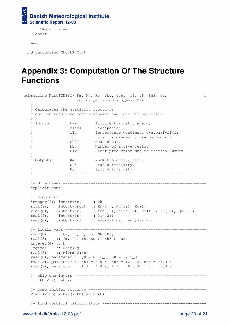
Appendix 3: Computation Of The StructureFunctions

subroutine PartIIDiff( Km, Kh, Ks, tke, diss, rT, rS, Sh2, kb, &eddydif_max, eddyvis_max, Piw)

!---------------------------------------------------------------------------! Calculates the stability functions! and the resulting eddy viscosity and eddy diffusivities.!! Inputs: tke: Turbulent kinetic energy.! diss: Dissipation.! rT: Temperature gradient, g*alphaT*dT/dz! rS: Salinity gradient, g*alphaS*dS/dz! Sh2: Mean shear.! kb: Number of active cells.! Piw: Shear production due to internal waves.!! Outputs: Km: Momentum diffusivity.! Kh: Heat diffusivity.! Ks: Salt diffusivity.!---------------------------------------------------------------------------

!- directives --------------------------------------------------------------implicit none

!- arguments ---------------------------------------------------------------integer(4), intent(in) :: kbreal(8), intent(inout) :: Km(1:), Kh(1:), Ks(1:)real(8), intent(in) :: tke(1:), diss(1:), rT(1:), rS(1:), Sh2(1:)real(8), intent(in) :: Piw(2:)real(8), intent(in) :: eddydif_max, eddyvis_max

!- locals vars -------------------------------------------------------------real(8) :: t2, ss, D, Nm, Nh, Ns, fcreal(8) :: fm, fs, fh, Rg_t, Sh2_t, N2integer(4) :: klogical :: CheckRgreal(8) :: PiwKm(2:kb)real(8), parameter :: y0 = 0.16_8, D0 = 24.0_8real(8), parameter :: nn1 = 8.0_8, nn2 = 12.0_8, nn3 = 75.0_8real(8), parameter :: ff1 = 4.0_8, ff2 = 60.0_8, ff3 = 15.0_8

!- skip one-layers ---------------------------------------------------------if (kb < 2) return

!- some initial settings ---------------------------------------------------PiwKm(2:kb) = Piw(2:kb)/Km(2:kb)

!- find vertical diffusivities ---------------------------------------------



! k = 1 (dummy values, not used anywhere) .................................

! Do the rest of the water column k=2,kb ..................................do k=2,kb

!- dynamical turbulent time scale squared, t2t2 = (tke(k-1)/diss(k-1) + tke(k)/diss(k))**2

!- total shear and Rg:N2 = rT(k) - rS(k)Sh2_t = Sh2(k) + PiwKm(k)Rg_t = min( N2/max(Sh2_t,tinyv), Rg_max )

!- no mixing if critical Rg is exceeded:call CheckRgCrit(rT(k), rS(k), Rg_t, CheckRg)if (CheckRg) then

Km(k) = laminarvisKh(k) = eddydif_minKs(k) = eddydif_min

!- mixing if critical Rg is not exceeded:else

fh = -pi2*pi3*t2*rT(k)fs = pi3*pi3*t2*rS(k)fm = y0*t2*Sh2_t

D = D0 &+ ((d1*fh + d2*fs + d8)*fh + (d3*fs + d9)*fs + d13)*fm &+ ((d4*fh + d5*fs + d10)*fh + (d6*fs + d11)*fs + d14)*fh &+ ((d7*fs + d12)*fs + d15)*fs

if (D >= zero .and. D < tinyv) thenD = tinyv

elseif (D < zero .and. D > -tinyv) thenD = -tinyv

endif

!- momentum:Nm = nn1*(nn2 + (a1*fh + a2*fs + a4)*fh + (a3*fs + a5)*fs)/nn3

!- heat:fc = ff1*(ff2 + b3*fm + b4*fs +b5*fh)/ff3Nh = pi4*(one + b1*fs + b2*fh)*fc

!- salinity:Ns = pi1*(one + b6*fs + b7*fh)*fc

!- eddy diffusivity normalised w/ structure function=1, ss:ss = tke(k-1)**2/diss(k-1) + tke(k)**2/diss(k)

!- vertical diffusivities:Km(k) = min( max(ss*Nm/D, laminarvis), eddyvis_max )Kh(k) = min( max(ss*Nh/D, eddydif_min), eddydif_max )Ks(k) = min( max(ss*Ns/D, eddydif_min), eddydif_max )

endif

enddo

end subroutine PartIIDiff


Danish Meteorological Institute - DMI · Danish Meteorological Institute Scientiﬁc Report 12-03...

Documents

Transcript of Danish Meteorological Institute - DMI · Danish Meteorological Institute Scientiﬁc Report 12-03...