DANISH METEOROLOGICAL INSTITUTE

————— TECHNICAL REPORT ———

02-10

A research version of the STRACO cloud scheme

Bent Hansen Sass

COPENHAGEN 2002

ISSN: 0906-897X (printed version) 1399-1388 (online version)

A research version of the STRACO cloud scheme

Bent H. Sass

Danish Meteorological Institute

1

1. IntroductionThe goal of physical parameterization in numerical models of the atmosphere is to ad-equately describe the physical processes in the atmosphere. These processes occur toa large extent on a sub-grid scale which the model cannot otherwise compute due to alack of model resolution.

The present report is concerned with an important and complex part of physical param-eterization, namely the description of subgrid scale condensation of water vapor with as-sociated phase changes, and the formulation of precipitation plus evaporation processes,hereafter referred to as CCPE processes = (Convection -Condensation - Precipitation -Evaporation). A specific scheme for describing these processes will be documented indetail. This scheme is being developed in collaboration with the HIRLAM community(Lynch et al., 2000), and a version of the scheme is used operationally at the DanishMeteorological Institute (DMI). The scheme has novel features related to cloud param-eterization and the treatment of precipitation release.

When decribing cloud physics in atmospheric models an important point is that thecondensation and precipitation processes are strongly dependent on both resolved scalemotions described by the model dynamics and subgrid scale motions on all scales fromthe convective cloud motions over the full depth of the troposphere down to the smallestturbulent scales. In the present context this means that the computations related tothe CCPE processes are dependent on the formulation of the model dynamics and tur-bulence of the HIRLAM forecasting system (Sass et al., 2002; Unden et al., 2002) Thevertical transport processes are by far the most important to parameterize due to thepresence of the earth’s surface as a boundary for vertical fluxes and the large verticalgradients of most meteorological parameters. However, when approaching the scale ofabout 1 km , the socalled cloud resolving scale, the importance of the lateral subgridscale transports increases.

When developing a parameterization of CCPE processes several problems or questionsemerge:It is a question how the whole range of subgrid scale transports can be adequatelydescribed. Practically all schemes developed for atmospheric models in the past dis-tinguish between ‘turbulence parametrization’ and ‘convection parameterization’. Theformer describes the small scale transports up to a dimension of a few hundred metreswhile the latter describes vertical transports extending up to the full depth of the tropo-sphere. It is often questioned whether the turbulence scheme and the convection schemeeach describe separate scales of the subgrid transports leading to worries about possible‘double counting’ the heat and moisture transports.

It is normally assumed that parameterization can be made from model parameters de-fined for a given grid square or an air column vertically above a surface grid square.However, this assumption becomes increasingly problematic as the grid size becomessmall. This problem shows up when treating deep convection since a convective cloudsometimes move horizontally by more than one grid distance during its evolution cycle.A similar problem occurs in relation to precipitation release from high elevations wherethe precipitation particles may travel several grid distances ‘downstream’ before reach-ing the ground. Also the assumption in many large scale models that an ensemble of

2

convective clouds exist in balance with the large scale forcing breaks down as the gridsize is reduced towards the cloud scale. Hence it appears that the parameterization ofthe CCPE processes in connection with convection are particularly difficult.

The condensation processes in a statically stable atmosphere inside a grid box desribedby a ‘stratiform’ condensation scheme is also influenced by subgrid scale motions giv-ing rise to subgrid scale condensation (partial cloud cover). As the grid size becomessmaller, however, the amplitude of the subgrid moisture variations becomes smaller andmust decrease towards zero as the grid size goes towards zero. One may claim that thesubgrid parameterization should automatically include assumptions about the scale de-pendency of the process description even if it is difficult to prove the validity of a specificscale dependency. It is often difficult to validate which formulations should be preferredby means of solid observational evidence. The results of very high resolution large-eddysimulations might be a tool to validate proposed scale dependent formulations. Thealternative is to make specific model tuning of various parameters when changing themodel resolulion. In recent years international comparisons have been useful as a guid-ance, e.g., the GEWEX (Global Energy and Water Cycle Experiment) cloud systemstudy (GCSS).

There have been many approaches during the past decades to describe the processesconnected to clouds and condensation. This is partly because of the large amountof subjects involved in the CCPE process description. In the HIRLAM community arevview has been written on the use of convection schemes in mesoscale models (Bister,1998). One trend has been to apply mass flux concepts to parameterize convection. Itmay be argued that a mass flux approach is more physically based than are formulationsrelying on alternative approaches. However, the details of the processes governing theevolution of mass fluxes are not well known.

For the socalled stratiform condensation process in a statically stable atmosphere the as-sumtions on the character of the subgrid scale condensation influences the microphysicsincluding precipitation release.

Section 2 to section 4 contain a documentation of a research version of the operationalcloud- and condensation scheme used at DMI. The scheme is named STRACO whichstands for ‘Soft TRAnsition COndensation’ (gradual transitions between convective andstratiform regimes).The prognostic model variables used by the scheme comprise specific humdidity q, cloudcondensate qc, temperature T , the horizontal wind components u and v and the surfacepressure ps. In addition, a vertical velocity is used.Section 2 is devoted to a description of the convection scheme. Section 3 is concernedwith the subgrid scale cloud parameterization and the ‘stratiform’ condensation process.Section 4 contains a desciption of the microphysics involved, including parameterizationof phase changes and physics related to precipitation release. A brief discussion andconcluding remarks are finally provided in section 5.

3

2. Parameterization of convectionCurrently the operational convection scheme is based on a moisture budget closure. Thisimplies that the moisture source from the model’s dynamics and turbulence scheme dur-ing a physics time step may be redistributed in a convective air column leading to heatingand moistening. For the basic redistribution to become active it is assumed that thetotal vertically integrated supply of humidity should be positive. In this respect thescheme may be viewed as a further development of ideas expressed by Kuo (1974). Thereasoning behind this type of closure is that a substantial convective activity needs amoisture source (moisture ‘convergence’) to be sustained. In the present scheme thetreatment of the moisture convergence includes the effect of surface evaporation flux.The vertical transports include a formulation of the vertical redistribution of cloud con-densate since ‘prognostic cloud water’ is a feature of the scheme.Convection can start from any level in the atmosphere provided that the onset of con-vection is supported by the model’s cloud ascent formulation. Some convection schemestreat only deep convection originating from the lowest model layer.Also fluxes of moisture and heat across the interface to the stable atmosphere abovethe convective entity are taken into account. Moreover, the precipitation release formu-lation differs radically from the parameterization in schemes which do not have ‘cloudcondensate’ as a prognostic variable.

Before describing the equations connected to the convective closure the method to assessthe moist convective part(s) of the atmosphere will be described.

2.1. Determination of convective entities

The convective part of the STRACO scheme defines vertical sections of the atmospherewhich form convective ‘entities’. The vertical extent of a convective entity is determinedby adiabatic cloud ‘parcel’ lifting including latent heat release. The cloud parcel starts atthe bottom of a new part of the atmosphere to be investigated for convective instability,using a trigger perturbation temperature and specific humidity, respectively. A weakresolution dependence of the perturbations is suggested. The perturbations are definedin (1) and (2). It is seen that the perturbations goes to zero as the grid size goes towardszero which is the governing constraint.

∆Tper =1

a1 + a2 ·√

DTD

(1)

∆qper = a3 · qk ·√

D

DT(2)

a1 = 0.6K−1 and a2 = 0.5K−1, a3 = 0.02 DT = 1.0 · 104m. D is the model grid size(m). qk is the specific humidity at the bottom of the convective entity considered.

The convective parcel ascent is carried out by assuming that the convective air parcelremains saturated at the saturation specific humidity of the convective air parcel tem-perature which evolves by the adiabatic lifting process and a ‘dilution’ process. Thisis a volumetric mixing fraction per unit length of vertical ascent. This environmental

4

mixing process normally tends to cool the convective air parcel by evaporation of cloudparcel cloud condensate into dry environmental air. Such process is often quite powerfulto reduce the buoyancy of the convective cloud and may strongly reduce the verticalextent of convection which stops as the cloud buoyancy becomes negative.

A volume fractional entrainment εe per unit length of vertical parcel ascent is tentativelydescribed according to the equation below.

εe =(Kε0 +

Kε1

Ri∗

)·( z

(Kε3 + z)

)· D0

D(3)

In (3) Ri∗ is a Richardson number which enables that effects of wind shear is in-corporated. It is argued that increasing wind shear gives rise to more mixing of theconvective cloud with the environments.

Ri∗ =(θ

g|∂V

∂z|2

)−1 ·(Kε2 + |∂θ

∂z|)

In (3) Kε0 = 1.3 · 10−4m−1 , Kε1 = 7.5 · 10−4m−1.The second brackets of (3) expresses a height dependency of the entrainment processbeing dimensionless and increases from zero at the surface towards 1 at great heights.Kε2 = 1.0 · 10−4K · m−1 and Kε3 = 500m.

convective cloud

lateralmixing

topmixing

dmix

Dcld

lateralmixing

cloud scale

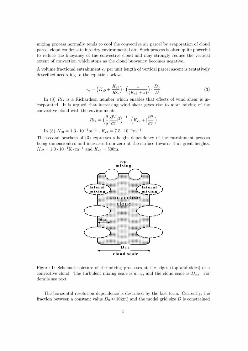
Figure 1: Schematic picture of the mixing processes at the edges (top and sides) of aconvective cloud. The turbulent mixing scale is dmix, and the cloud scale is Dcld. Fordetails see text

The horizontal resolution dependence is described by the last term. Currently, thefraction between a constant value D0 ≈ 10km) and the model grid size D is constrained

5

to be no less than 1.If it is maintained that the parameterized convection should describe effects of subgridscale features being 1-2 orders of magnitude smaller in areal extent than the grid square,it is reasonable to assume that the dimension of the parameterized convective clouds(parcels) decreases roughly proportional to the grid size. It seems reasonable to assumethat the ratio between the surface and the volume of a convective cloud increases asthe horizontal dimension of the cloud decreases. For a ball-shaped cloud the ratio goesto infinity and is inversely proportional to the size of the convective cloud. As a con-sequence one might expect that the dilution process is becoming more efficient at highmodel resolution since the ratio Dmix/Dcld between the characteristic turbulent scaleDmix and the size Dcld of the cloud increases (see figure 1). As a first approximationit is therefore assumed that the volumetric dilution becomes inversely proportional togrid size which is expressed by the last term of eq. (3). An important consequence ofthe resolution dependent dilution is that the vertical extent of parameterized convectionwill automatically be reduced as the model grid size is reduced. As a consequence theparameterized ‘deep convection’ will automatically tend to be ‘switched off’.

Model experimentation confirms that there can be a pronounced and sometimes sub-tle interaction between a model’s turbulence scheme and convection scheme. For thepresent model it has been found that it is beneficial to impose a regulating criterionwhich controls the depth of a convective entity for a rather weak integrated moistureconvergence. A maximum depth Dcv in Pa of a convective entity is determined by

Dcv = C1 + C2 · Q∗ (4)

In (4) Q∗ is the moisture accession, if positive (kg · kg−1 · s−1 Pa), otherwise it iszero. More precisely , it is the average specific humidity rate of change over the convec-tive entity times the pressure thickness of the convective entity in Pa. C1 = 1.25 · 104PaC2 = 4.0 · 107s · kg · kg−1 The significance of the above formula is for cases where thevertically integrated moisture accession is small.

The level of non-buoyancy determines a transition to the stable atmosphere above. Theeffect of overshooting eddies penetrating into the stable layer above the moist unstableatmosphere is parameterized and a depth of this ‘extension zone’ is estimated (Sass,2001). It is at least one model layer and is limited to be at most 25 hPa thick. Theconvective transports of heat and moisture, including cloud condensate, across the in-terface between the moist unstable and the stable atmosphere, is often termed ‘shallowconvection’. This effect is also parameterized when a deep moist convective atmosphereis involved (see below).

6

2.2. Convective equations

The relevant equations describing the processes in connection with convection are de-scribed below:(

∂q

∂t

)ADC

=(

∂q

∂t

)AD

(1 − δ∗) + QaβFq

Fq

δ∗ + Kcqc(qs − qe) + Sq + Epc (5)

(∂qc

∂t

)ADC

=(

∂qc

∂t

)AD

+ Qa(1 − β)Fc

Fc

δ∗ − Kcqc(qs − qe) + Sc − Gpc (6)

(∂T

∂t

)ADC

=(

∂T

∂t

)AD

+L′

cp

(Qa(1 − β)

Fh

Fh

δ∗ − Kcqc(qs − qe)

)+ ST − L′

cpEpc (7)

The left hand sides of these equations express the combined effect of both dynamicaladvection, turbulence and convection. ∂

∂t()AD signifies a tendency excluding convection.Qa is the total moisture accession per unit mass and time in the convective cloud. L′ andcp represent the specific latent heat of fusion or sublimation, depending on the micro-physical conditions, and the specific heat capacity at constant pressure, respectively (seesection 4).

Fh is a function describing the vertical variation of convective heating.

Fh = Tvc − Tve + εT (8)

Fq is a function describing the vertical variation of convective moistening.

Fq = qsc − qe + εq (9)

Fc is a function describing the vertical variation of convective condensate supply.

Fc = qcc + εc (10)

In the above equations for Fh, Fq and Fc index v stands for ‘virtual’. Index e means‘environmental’ (outside clouds). F stands for a vertical average value for the convectivecloud. Finally, c-index means a value applicable to cloud and s signifies a saturationvalue. The constants εT , εq, εc are currently set to zero.

The parameter β is a moistening parameter (Kuo, 1974). It represents moisteningdue to convective transports, without condensation. In the present scheme, contraryto models without prognostic cloud condensate, moistening can take place also fromevaporation of cloud condensate. As a consequence, this β-term is considered of reducedimportance in the present scheme.

β =

1 −∑jtop

j=jbotqqs

∆p

pjbot − pjtop

n1

(11)

In (11) p represents ‘pressure’, and jbot and jtop are the model level numbers for thebottom and top of convection, respectively. Currently n1 is set to a value of 2.The parameter δ∗ is an important one, because it determines a link between convectivemoisture transports on one hand and turbulence plus dynamics effects on the other.

δ∗ =(

∆pc

p00

)n2

(12)

7

In (12) ∆pc is the total depth of the convective entity considered, and p00 is a constantcloud depth used for scaling. Currently p00 = 2 · 104 Pa, n2 = 1. δ∗ is constrained tobe no larger than 1. The effect of this formulation is that δ∗ goes to zero for extremelyshallow phenomena. A very small δ∗ means that the convection scheme is decoupled asis reasonable in the limit of very shallow phenomena and high resolution where dynamicsand turbulence should suffice.

The third term in the main equations involving (qs − qe) is an evaporation /sublimationterm of cloud condensate. (Kc is a constant). A similar formulation, involving cloudcover as the leading term in place of qc, has been used by others, e.g., (Tiedtke, 1993)in the ECMWF cloud scheme. The parameterization of this term is difficult, partlybecause of the problem to describe the surface area of clouds and the degree of mixingat the edges of the clouds which are in a subsaturated environment.

The fourth term in the same equations, involving Sq, Sc and ST respectively, de-scribes the effect of fluxes of heat and moisture across the interface between a moistconvective atmosphere and the stable atmosphere above. For example, this parameteri-zation is needed at stratocumulus cloud tops unless the turbulence scheme is specificallydesigned for computing such fluxes. We let the convection scheme describe the effectof larger eddies in an environment where condensation takes place. The computationsmake use of the cloud parcel ascent computation of the convection scheme. Physicallywe may think of the heat- and moisture transports as accomplished by mainly the largereddies penetrating through the stable layer on the top of a cloud layer. The penetrationof these eddies into the stable layer can be estimated from the cloud parcel ascent. Theobservational and modelling evidence that stratocumulus are associated with a substan-tial entrainment of (dry) air from the stable layer into the cloud (Nicholls and Leighton,1986; Duynkerke et al., 1995) makes it reasonable to assume that this hypothesis of‘overshooting’ eddies as the mechanism for entrainment of dry air is a reasonable con-cept. We denote by wb a characteristic vertical velocity of convective motions in thecloud right below the cloud top and will estimate a distance De of penetration into thestable layer.

This depth is estimated as follows: From dimensional analysis it has been argued thatthe vertical velocity wr of an idealized thermal depends on its size r, the dimensionlessbuoyancy B of the ‘bubble’ and the acceleration of gravity g (m s−2) according thefollowing combination (Rogers and Yau, 1989).

wr = cb

√gBr (13)

In (13) B is the virtual temperature difference between the cloud parcel and envi-ronment, divided by the environmental temperature. cb =1.2. Choosing r = 50 m asrepresenting the dimension of convective eddies near cloud top we get

wb = w0 ·√

B

w0 =≈ 27 m s−1.B is computed in the cloud ascent of the convection scheme (see section 2.1).

We estimate the maximum penetration depth De from the deceleration in the stablelayer. Utilizing the start velocity of wb for the deceleration we get

8

De = w0

√B · T

g|γc − γ| (14)

In (14) De is in metres, T is temperature (K), γc in K m−1 is the lapse rate associatedwith moist adiabatic ascent (γc > 0) and γ in K m−1 is the ambient lapse rate in thestable layer. It is demanded that γ < γc. A numerical security computation has beenimplemented to avoid extreme behaviour if the two lapse rates become almost equal,and the penetration is not allowed to exceed a depth corresponding to 25 hPa.

A maximum fluctuation s′ of the variable s possible at the interface between cloud andthe stable layer is estimated to be approximately equal to the increase above the values− at the interface on the cloudy side up to the value se at depth De into the stablelayer. The value se is estimated from the mean gradient of the variable at cloud top.More specificly, it is assumed that the flux at the cloud top of the scalar s is a factor wtimes s′ where w is a velocity scale. It is reasonable to assume that the velocity scale wis closely linked to a typical convective cloud velocity at the top of convective clouds. Itis therefore argued that a reasonable estimate is

w = w1 ·√

B (15)

In (15) w1 = 0.15m · s−1 has been determined on the basis of numerical experimen-tation.

The sensible heat flux FH (J m−2 s−1) at the level of transition between cloud and thestable layer is computed according to

FH = ρcp · w · De · ∂θ

∂z(16)

In (16) cp is the specific heat capacity at constant pressure. ρ is air density, θ ispotential temperature.

Similarly we get for the moisture flux of total specific humidity qt (kg · m−2 s−1) atthe transition level

Fqt = ρ · w · De∂qt

∂z(17)

We assume that the fluxes of heat and moisture determined from the above formulasare distributed linearly with height in the convective cloud of depth D− and in a stablelayer D+. The latter should approximately be equal to De apart from the constraintsset by vertical resolution. If De is larger than the depth of one model layer above cloud asufficient number of levels are included to exceed De. Currently, the specific humidity qand cloud condensate qc are processed independently according to the method describedabove, but the flux of the moist conserved variable of ‘total specific humidity’ is thenalso linear, which preserves moisture structures in a well mixed cloud.

A semi-implicit treatment of the scheme has been introduced to reduce the risk of noiseor instability when computing updates of the prognostic variables. It involves partialderivatives of the fluxes described above, as well as the associated layer depths.

9

Finally, the terms involving Gpc and Epc concern generation and evaporation of convec-tive precipitation, respectively (see section 4).

The equations above are applied in the layers of the convective entities while the strat-iform condensation applies to the remaining parts of the atmosphere.

3. Cloud cover and subgrid scale condensationIn the previous section the equations governing the subgrid scale vertical convectivetransports of heat, humidity and cloud condensate have been described. While theseequations describe the evolution of temperature (T ), specific humidity (q) and cloudcondensate (qc) in a grid box for the convective part of the atmosphere the distributionof humidity within the grid box has not yet been treated. It is natural to describethe humidity variation by a statistical probability distribution function (PDF) whichwill define both saturated and unsaturated portions of the grid box. By definition, thefractional cloud cover is the saturated fraction of the grid box with cloud condensate insome concentration. Hence cloud cover will be defined by the PDF which needs to bedefined not only for the convective parts of the atmosphere, but also for the stratiformparts. There are substantial differences between the convectively unstable and the stablestratiform regimes as will be described below:

We first consider the problem of defining convective cloud cover. For clarity an ‘overline’symbol is used in this section for grid box average values, q for specific humidity, qc forspecific cloud condensate and qt = q + qc for total specific humidity. The prognosticmoisture variables q and qc have known values at a given time step of a model run. Fur-thermore, the relevant saturation specific humidity to describe supersaturation is qs(Tc),which is the saturation specific humidity valid for the convective cloud temperature Tc.This temperature is available from the convective cloud ascent model. One may arguethat a probability function describing the variation of total specific humidity around thegrid box average value defines the supersaturation in the grid box. In the convectivesituation the challenge is that the distribution of total specific humidity can vary a lotacross the grid box, and the moisture distribution may be quite asymmetric. This isbecause moisture is exchanged over large depths in the atmosphere. Also temperaturevaries to some extent. A true description of supersaturation taking into account bothtemperature and moisture variations is therefore very complex. The extreme situationwhere cloud cover becomes 100 % may then be a combination of saturated fractions ofthe grid box with different temperatures. In the present description we have alreadyintroduced the convective cloud temperature Tc which is generally higher than the gridbox mean value T . However, in order to simplify cloud cover computations near gridbox saturation, and in order to avoid a too high level of complexity, it is demandedthat the convective cloud temperature goes towards the grid box mean value T whenq goes towards qs(T ). This means that the preliminary convective cloud temperatureTc is corrected close to grid box saturation conditions. This is done when the relativehumidity exceeds 1 − Ast where Ast is defined later in this section in the context ofstratiform condensation.

T ′c = Tc +

( q

qs(T )+ Ast − 1

Ast

)2 · (T − Tc) (18)

10

In (18) T ′c is the corrected convective cloud temperature.

After this simplification we try to describe the probability function defining the variationof total specific humidity by means of a piecewise rectangular probability density func-tion. The most simple formulation involves 2 rectangular boxes which allows for a simpleasymmetric PDF. This type of formulation has been used in the past. The formulationbelow, however, represents an enhancement consisting of 3 boxes when qt < qs(Tc). Theapplication of 3 boxes in a rather dry atmosphere is consistent with a simple conceptualpicture of convective clouds with a large specific humidity embedded in an environmentwith a fairly homogeneous humidity. Under these conditions a double-peaked PDF maybe expected which fits with a 3-box structure (see figure 2).

The 3 boxes have amplitudes ψ1, ψ∗ and ψ2, respectively (figure 2). The amplitudes areyet unknown, but may be determined by solving the equations (21), (22) and (23) forthe situation that qt < qs(Tc). These equations have a solid basis. Eq.(21) defines thatthe total integral of the PDF equals 1 when integration is done over the entire humidityspectrum. Eq.(22) expresses that the average value of qt as determined from the PDFshould be equal to the grid box total specific humidity. Eq.(23) is a computation of thegrid box mean cloud condensate from the PDF. The integration limits qmin and qmax

have so far not been defined.

The strategy is to parameterize qmin which appears as a free parameter. Based onexperimentation qmin is currently defined as follows:

qmin =

{qmin1 if qt < qs · (1 − Ast)qmin1 · (1 − y) + qmin2 · y if qs · (1 − Ast) ≤ qt ≤ qs

y =( qt

qs(Tc)+ Ast − 1

Ast

)2

qmin1 = qt(1 − Cw1qc

qs(Tc)− Cw2) (19)

qmin2 = qs(Tc) − Cw1 · qc (20)

In (19) and (20) Cw1 = 4 and Cw2 = 0.02The interpolation formulas for qmin makes it possible to obtain a symmetric PDF at

qt = qs(Tc). The associated range of variability at this point is qt − qmin = 4qc. Thisresult may be shown by integration of the equation for cloud condensate (23) below.

Then the equations (21),(22) and (23) constitue a system of 3 equations with 4 unknownsnamely the amplitudes ψ1,ψ∗, ψ2 and the integration limit qmax. By formally solvingthe system of 3 equations it is possible to express qmax by means of ψ∗ and the otherknown parameters. This solution is specified in (25). At this stage it is possible tospecify the amplitude ψ∗ with some freedom as a tuning parameter under the restrictionthat qmax is larger than qs. This leads to a limit ψ∗l on ψ∗ according to eq.(26). It isnoted that the convective cloud cover fcv is obtained by integrating ψ2 which operatesover the saturated part of the grid box.

11

∫ qt

qmin

ψ1dqt +∫ qs

qt

ψ∗dqt +∫ qmax

qs

ψ2dqt = 1 (21)

∫ qt

qmin

ψ1 · qt · dqt +∫ qs

qt

ψ∗ · qt · dqt +∫ qmax

qs

ψ2 · qt · dqt = qt (22)

∫ qmax

qs

ψ2 · (qt − qs)dqt = qc (23)

fcv =2qc

qmax − qs(24)

qmax = (b1 + b2ψ∗)/(b3 + b4ψ∗) (25)

b1 = (qt − qmin) · (qs + 2qc) − 2qs · (qt + qc)

b2 = qs · (qs − qt) · (qs + qmin + 2qt)

b3 = qt + qmin − 2q

b4 = (qs − qt) · (qs − qmin)

The limit ψ∗l of ψ∗ is

ψ∗l = (b3qs − b1)/(b2 − b4qs) (26)

Hence the applicable values of ψ∗ may be written as

ψ∗ = δψ · ψ∗l

It may be determined whether δψ must be chosen larger than or smaller than 1 bydifferentiating with respect to ψ∗

∂(qmax − qt)∂ψ∗

in the point ψ∗l. In this way it may be concluded that δψ should be smaller than 1(first case) if

b2(b3 + b4ψ∗l) − b4(b1 + b2ψ∗l) < 0 (27)

On the other hand, δψ should be larger than 1 if the sign of the expression in(27) is positive (second case). Tentatively the values δψ = 0.07 (first case) and 1.07(second case) have been set which appear to give reasonable results. The selection ofoptimal values, which may be determined from a more involved computation, requiresexperimentation with a given model.

12

Hence it may be concluded that the above solution allows for some freedom regardingthe choice of qmin and ψ∗. Having made an appropriate choice the unknowns are thenψ1, ψ2 and qmax, and the cloud cover fcv may be computed from (24) and (25).

For humid conditions qt > qs(Tc) it is assumed that the PDF is symmetric and that thehumidity variation covers at least the range from qs(Tc) to qt. Integrating the equationfor cloud condensate (23) then gives for the range Ac defined from qmin = qt · (1 − Ac)

Ac =−b6 +

√b26 − 4b5b7

2b5(28)

In (28)

b5 =12q2t

b6 = qt · (qt − qs − 2qc)

b7 =12(qt − qs)2

The cloud cover fcv becomes

fcv = Min((qt − qs)

2Acqt

, 1)

(29)

In the stratiform regime we need to define both cloud cover and the stratiform condensa-tion process. The generally smaller vertical scales and larger horizontal scales associatedwith stratiform condensation makes it reasonable to assume a smaller spatial variationand a symmetric PDF of qt as an approximation to the true PDF. The PDF, which isrectangular, is shown schematically in figure 2 (to the right). qs is now equal to the gridbox saturation value qs(T ). Again the temperature variation in the grid box is neglected.The assumption is also made that clouds extend vertically from the bottom to the topof a model layer. These assumptions are quite common among modellers (Sundqvistet al., 1989; P.J.Rasch and J.E.Kristjansson, 1997). The amplitude ψ is evidently givenby (30)

ψ =1

2 · (qmax − qt)(30)

The maximum value qmax of total specific humidity in the stratiform case is formallywritten

qmax = qt · (1 + Ast) (31)

The dimensionless amplitude Ast is determined from a time dependent equation tobe described below (see equation 35).At first it is noted that, for a given value of Ast, the equilibrium cloud condensate valueqceq as determined from the PDF, may change from the current value qc as a result of

13

changing temperature and specific humidity during the run. The system of equations(32) and (33) defines the condensation process to establish an equilibrium among themodel variables by a first order adjustment. Higher accuracy can be obtained if (32)and (33) are applied several times in an iterative fashion. In practice, it has been chosento apply a relaxation towards the equilibrium using a small relaxation time period. Atleast half of the supersaturation is removed per time step. However, full adjustment ina time step is done in the case of grid box supersaturation.

∆qst =(qc − qceq)

1 + f · L′cp

(∂qs

∂T

) (32)

qceq = 0.5 · ψ · q2s + ψ · qmax · (0.5qmax − qs) (33)

In (32) ∆qst refers to the change of specific humidity during the adjustment process.f is the current value of the fractional cloud cover. L

′is the specific latent heat as a

function of temperature (to be defined in the next section). In (33) the˜symbol appliesto preliminary model variables to be adjusted during the condensation process.

In this case the cloud cover fst associated with the equilibrium density function is:

fst =1 + Ast − qs(T )

qt

2Ast(34)

In general, the dimensionless amplitude Ast describing the variation of total specifichumidity is not constant, but is a function of model resolution, space and time. Atentative time dependent formulation of Ast is expressed in (35) which is intended to

ψ

qmin

q q q t s max

q q qmin t max

ψ

qs

Figure 2: Two examples of piecewise rectangular probability density functions of totalspecific humidity. The dark dotted regions describe supersaturated cloudy parts. Theleft figure applies to convective conditions and the figure to the right to stratiform con-ditions. qmin is the minimum value of total specific humidity with non-zero probabilityand qmax is the maximum value. qt is the grid box value of total specific humidity andqs is the saturation value for cloud computations. See text for details

14

describe at least qualitatively the effect of model resolution, elevation above the surface,stationary forcing effects, unsteady flow effects and the effect of precipitation release.The reasoning behind each term of the equation is described below:

∂Ast

∂t= −K1 · (Ast−Acli)+

K2

qt· |∂qt|

∂t· (Amax−Ast)+

K3

qt·Min(

∂qc

∂t prc, 0.) · (Ast−Amin)

(35)In (35)

Amax =α1 + α2 · (1 − ( p

ps)3)

(α1 + α2) · (1 +√

α3D )

(36)

Currently α1 = 2 , α2 = 9, Amin = 0.005 α3 = 3.6 · 105m K1=4.63 · 10−5 · s−1 K2 =3, K3 = 9. The maximum allowed value Amax of Ast in (35) describes effects of elevationabove surface and of model grid size. In (36) p and ps are model level pressure and surfacepressure, respectively. The term involving p/ps describes a significant reduction of Ast

towards the surface. A similar effect have been included by others (Sundqvist et al.,1989). The term involving grid size D in the denominator of (36) implies that Ast goestowards zero for the grid size going to zero. Obviously this is reasonable in a continuousformulation. Results from the litterature (Redelsperger and Sommeria, 1986) emphasizethe virtues of having a subgrid scale parameterization of condensation even at horizontalresolutions of a few kilometres grid size. This is consistent with results from large eddysimulations in recent years, indicating that subgrid scale variability is well pronouncedat a grid size of few kilometres. The square root in the denominator is used in order toincorporate the effect that subgrid scale variations are significant already at a grid sizeof a few kilometres.

The second term of (35) is a crude parameterization of nonstationary flow effects. Theterm expresses that the change of Ast towards the maximum allowed value is proportional(dimensionless factor K2) to the relative rate of change of total specific humidity. Sucha formulation is reasonable to the extent that resolved scale advections are reflected alsoin a subgrid scale variation, that is, augmented and reduced advections compared togrid box mean value exist inside the grid box.

The first term describes a relaxation towards the value Acli which stands for a ‘climatic’type of stationary forcing. Currently the value of Acli is a fixed fraction of Amax (Acli =0.75 · Amax). A more refined treatment could take into account local stationary forcingeffects, e.g., due to varying topography. The relaxation factor corresponds to an e-folding time og 6 hours. The formulation inplies that, in the absence of non-stationarityand precipitation release the amplitude Ast approaches Acli exponentially with the givene-folding time.

Finally the last term which is qualitatively similar in appearance to the second term,expreses always a reduction of Ast towards a minimum value Amin. (∂qc/∂t)prc expressesthe reduction rate of cloud condensate due to precipitation release in the grid box.The reasoning behind this term is the following: Consider a saturated grid box withcloud condensate in spatially varying amount consistent with a given positive valueof Ast. It is then possible that the cloud condensate will fall out if the precipitation

15

release parameterization is active, e.g. through a collission and coallescence processassociated with precipitation particles entering the grid box from higher altitudes. This‘sweepout’ process increases with increasing precipitation flux. The third term describesthat it is possible to reduce cloud condensate substantially during precipitation release(‘cloud thinning’) without substantial compensating condensation. Physically the cloudthinning process due to precipitation ‘sweepout’ seems realistic.

Finally, the non-stationary conditions as regards q, qc and T will sometimes lead tothe onset of stratiform condensation after convective conditions or vice-versa. Afterconvection is no more supported, the convective cloud may exist in a subsaturatedenvironment which is sufficiently dry such that subgrid scale stratiform condensation isnot supported. In this situation the evaporation terms, that is, the 3rd terms of (5), (6)and (7) describe also the evaporation of cloud condensate after convection.To describe the actual transitions the cloud cover f is made time dependent by relaxingtowards the equilibrium cloud cover feq which may be either a stratiform (fst) or aconvective equilibrium (fcv).

∂f

∂t= −Kf (f − feq) (37)

Currently K−1f = 900 s.

4. MicrophysicsThe model’s micro-physics concerns a parameterization of processes related to the for-mation/decay and fallout of precipitation particles. The microphysics represent thesmallest scales down to molecular processes in the atmosphere. An overview of centraltopics in cloud physics can be found in the litterature, see for example Rogers and Yau(1989).

Some of the equations described so far, e.g., (5), (6) and (7) already contain the effects ofmicrophysics. The terms Gpc and Epc describing precipitation release and evaporation ofprecipitation in the convective case need to be specified for these equations. The similarterms should be formulated in stratiform conditions. Also the effect of melting/freezingof precipitation needs to be specified. These effects are described below. The treatmentfollows closely the formulations by Sundqvist (1989) and Sundqvist (1993) except forsome extensions and few exceptions.

The potential advantage of having cloud condensate as a prognostic variable is thatcondensation and latent heating may occur without automatically giving rise to pre-cipitation release. For the present scheme this statement applies also to convectivecondensation. As described in section 2 the present treatment of convection allows forseveral convective layers or entities in a vertical air column. Stratiform condensationmay also occur in parts of an air column, and the cloudiness can be partial. This makesthe precipitation release parameterization and an associated description of evaporationof precipitation very complicated.Technically, this scheme separates between convective precipitation and stratiform pre-cipitation. Both may be present at the same time in a vertical column. A possible mutualinteraction between stratiform and convective precipitation fluxes is strongly restricted

16

in the current formulation. This is a common feature of most precipitation schemes usedin atmospheric models. The precipitation release formulas described below are basicallythe same for stratiform and convective precipitation release. The differences involvemainly different constants in the formulas. The precipitation flux from individual layersof the atmosphere are added down to the surface to produce surface precipitation rate.However, evaporation of precipitation is accounted for in this process. Also a treatmentof the transitions between water and ice phases makes it possible to distinguish betweenrain and snow.

We first describe the stratiform precipitation release. The rate of precipitation releasekg · kg−1s−1 is given by (38)

Gp = Φ · qc ·(1 − exp(− qc

f · µ)2)

(38)

In (38) f is the fractional cloud cover and qc is specific cloud condensate as in pre-vious sections. Φ is a rather complex function with unit s−1 and describes an inversetime scale associated with the precipitation release formulation.

Φ = Φ1 · Φ2 · Φ3

The first term Φ1 represents an inverse time scale depending on the dynamical modelstate represented by the vertical velocity ω in the pressure system. Φ1 decreases inproportion to −ω. The values of Φ decreases for non-positive ω and is constant (φst) forsubsidence conditions. It is limited to be no less than φ00. The term simulates the effectof precipitation particles being carried with the updraft velocity in the precipitatingclouds while it is advected also horizontally. The model resolved vertical velocity adds(subtracts) to the fall velocity, and therefore a longer time scale is associated with theprecipitation fallout under conditions of a sufficiently high vertical velocity. The termis novel and simulates the same effect as a prognostic precipitation field which may beadvected with the air flow while falling towards the surface with a characteristic velocity.This effect will get increasingly important at a high model resolution since, on average,larger vertical velocities will then be simulated.

Φ1 = φst + Kφ1ω∗(φst − φ00) (39)

ω∗ =

{0 if ω > 0ω if ω ≤ 0

ω = dpdt is the vertical velocity in pressure coordinates. Kφ1 = 0.02Pa−1 · s, φ00 =

1.0 · 10−5s−1, φst = 1.0 · 10−4s−1.

Φ2 = 1 +

√Pco

KB1

+ KB2δBF (40)

In (40) KB1 = 1.0 · 10−4kg · m−2 · s−1, KB2 = 4. The term involving KB1 describesthe effect of the collection process (collision and coalescence) on the precipitation release(Rogers and Yau, 1989). Pco is the precipitation intensity (kg · m−2 · s−1) per grid square

17

divided by the maximum of the fractional cloud covers present above the vertical levelconsidered. Hence Pco is an estimation of the precipitation flux per unit area enteringthe cloud at the local level considered.The second term, proportional to KB2 , describes the Bergeron-Findeisen effect (Berg-eron, 1935; Findeisen, 1938). This process enhances the precipitation release as icecrystals become present in a water cloud. The coefficient function δBF has been param-eterized according to Sundqvist (1993) and is given by (41) and (42).

δBF = δice · (1 − δice)∆Ewi (41)

δice = δice + (1 − δice) · Pice

Ptot(42)

In (41) and (42) δice is a basic function for the probability of ice crystals in clouds(Sundqvist, 1993). This formulation describing an increasing probability of ice crystals inthe interval between 273 K and 232 K is based on extensive statistics on the occurrence ofice crystals in clouds (L.T.Matveev, 1984). The functional form is given in the appendix.This function is also used to describe specific latent L′(T ) as a function of temperature,appearing in previous equations.

L′(T ) = Lv + δice · Li (43)

In (43) Lv is the specific latent heat of evaporation and Li is the specific latent heatof frezing/melting.

The ∆Ewi function is the difference in satuation vapor pressure over water and ice,divided by its own maximum value. Hence this function is dimensionless and has itslargest values between -10◦ C and -20◦ C. In is seen that the Bergeron-Findeisen termdescribes an enhanced precipitation release only if the ice fraction is less than 100 %and if precipitation as snow (ice) entering the layer is positive.The equation (42) describes a modified ice fraction when computing precipitation re-lease. The fraction of precipitation release from the layer being snow or ice will thenbe modified from δice to δice. A latent heating due to freezing associated with the mod-ified ice fraction is taken into account in the temperature equation. It is noted thatthis modelling of ice fraction increase as a result of the total precipitation flux fromabove (stratiform +convective) represents a weak coupling between the two precipita-tion streams, stratiform and convective precipitation, respectively. In all other aspectsthe two precipitation streams are currently described independently.

Finally, the term Φ is modelled as a dimensionless function. It has been introduced inorder to make precipitation release sufficiently efficient at very low temperatures below238 K (Kallen, 1996).

Φ3 =

1 if T > 2381 + 238−T

2 if T ∈ [230, 238]5 if T < 230

(44)

Looking back on on the precipitation release formula (38) the function in the bracketsimplies that the precipitation release becomes efficient as the specific cloud condensate

18

inside cloud (qc/f) reaches a magnitude of µ which is the second important function inthe description of precipitation release. This function is specified in (45), (49) and (47):

µ =µ1 · µ2

Φ2(45)

µ1 = µst + Kµ1 · ω∗(µst − µcv) (46)

µ2 = (1 − δice)2 + δice · ξ(T ) (47)

In (46) Kµ1 = Kφ1 and the functional form is similar to Φ1 except for the constants,that is, µst is a threshold value of cloud condensate in the case of ω∗ = 0. The maximumvalue allowed (µcv) equals the value normally used for the convection scheme for the caseof ω∗=0 (see 49). Currently µst = 5.0 · 10−4, µcv = 3.0 · 10−3.

The functions µ2 and Φ2 have been adopted from a previous formulation (Sundqvistet al., 1989; Kallen, 1996). The function of temperature µ2 has been found necessaryto describe a realistical amount of cloud condensate at low temperatures. The functionξ(T ) is given in the appendix.

For convective precipitation release similar formulas are used, except for some differencedescribed in (48) and (49).

Φ1cv = φcv + Kφ1 · ω∗(φcv − φ00) (48)

µ1cv = µst + Kµ3 · (µcv − µst) (49)

Kµ3 = Min(−Kµ1ω∗ + Kµ2B, 1)

In these equtions index ‘cv’ indicates use for convective conditions. In (48) thecurrently used value of φcv is 2.5 · 10−4s−1. The value of Kµ3 is constrained to be nolarger than 1. Kµ2 =250. The term involving buoyancy B as defined in section 2 isincluded to provide a continuous formulation between a stratiform and a convectiveregime. In most situations µ1cv = µcv.

The formulations of melting and of evaporation of precipitation are rather uncertain.Several formulations have been used in numerical models. Since less energy is involvedwith melting compared with evaporation or sublimation a very simple formulation isused for the melting process. As precipitation falls through a layer with temperatureabove 273 K while the precipitation as snow (ice) is present, the rate of melting M isdescribed according to the following equation (50)

M = Kml · cp

Li(T − Tml) (50)

Kml = 4.0 · 10−4 · s−1 The formulation defined by (50) describes in most situations com-plete melting in a layer of a thickness no more than a few hundred metres.

19

Finally, evaporation of precipitation takes place in subsaturated model layers. Asnoted by Tiedtke (1993) parameterizations of this process in operational numerical mod-els may be considered rather uncertain at present. This is reflected in various approachesgiving different results. Most formulations apply a formulation Ep (kg · kg−1 · s−1) pro-portional to the square root of precipitation intensity, e.g. Sundqvist (1989). Further,the evaporation should in some way depend on the atmospheric subsaturation. Somemodels use subsaturation qs − q as a basic parameter (Tiedtke, 1993), others relativehumidity (Sundqvist et al., 1989). Precise computations, using the basic physics, requireintegrations over droplet spectra, utilizing fall velocities and detailed computations ofthe diffusion process at the surface of the droplets, taking into account features suchas ventilation effects (Rogers and Yau, 1989). Currently (51) is used which depends onthe subsaturation qs − q and obeys a square root dependency on precipitation intensityat moderate to high precipitation fluxes, but allows for some increase of evaporationrate at low precipitation intensities. Curently Ke1 = 1.0 · 10−3, Ke2 = 1.0 · 103 andKe3 = 6.0 · 109. Optimal values of these coefficients are not well known at present.

Ep = Ke1 ·(qs − q)

(1 + L′cp

∂qs

∂T )·(√

P +Ke2P

(1 + Ke3P2)

)(51)

20

5. Discussion and conclusionsIt is clear from the presentation so far that that parameterization of CCPE processes innumerical models used for weather forecasting is complicated, for the following reasons:

There are still some general uncertainties on how to construct atmosphetic models in anoptimal way for a given set of applications. Apart from the numerical challenge it is stillnot known how to describe most accurately the subgrid scale fluxes of heat, moistureand momentum. A key problem is to describe all scales in a realistic way for models of acoarser resolution than the cloud resolving models. The turbulence formulation remainsa problem even in the cloud resolving models.

The complexity of the CCPE processes and the need to apply parameterizations whichare sufficently efficient from a computational point of view sets rather strong limita-tions on the methods which can be used. As a consequence, this often leads to thedevelopment of efficient parameterizations with rather many tuning constants as is thecase for the present scheme. Optimal values of tuning constants will depend on othercomponents of the meteorological model including the model dynamics.

For the present forecast model tuning of some parameters is likely to give more optimalresults, in particular as regards the formulations of cloud cover and precipitation releasewhich include new features. In addition, the turbulence scheme does currently not di-agnose moist unstable conditions in cloudy regions. This implies that the turbulenceintensity inside clouds is underestimated and is compensated for by the shallow con-vection parameterization of the convection scheme. In case that the turbulence schemeis upgraded to an adequate scheme for cloudy conditions some associated tuning mustbe expected with regard to the shallow convection parameterization. At a very highresolution also the amplitude of the moisture fluctuations described by the subgrid scalecondensation scheme should be made consistent with the moisture variation describedby the turbulence scheme.

In view of the difficulties involving tuning it is important to decide on a strategy whichfacilitates real progress in terms of more accurate parameterizations. It seems natural tochoose a strategy which splits up the CCPE processes in parts which can be studied moretheoretically in order to check, tune and possibly modify existing parameterizations.As an example, the significant spread of the results with different parameterizationsfor evaporation of precipitation calls for comparisons with detailed theoretical compu-tations based on size distributions of precipitation particles. This treatment shouldinclude varying fall velocity of cloud particles and a theoretically advanced treatmentof the diffusion proceses at the surface of precipitation particles, including ventilationeffects.

Another challenging problem is the forecasting of cirrus clouds. A correct determina-tion of these clouds seems to require that the water phase and the ice phase are storedseparately in the model. This means that ‘prognostic cloud condensate’ should be splitup into ‘prognostic cloud water’ and ‘prognostic cloud ice’. Ideally, a knowledge of thepresence of freezing nuclei is also necessary. Progress in this area may require a refinedaerosole treatment. The present scheme does not have such features and can be expectedto overestimate the occurrence of cirrus in some situations.

21

It is also relevant to carry out experiments where the performance of a turbulence schemecombined with the description of the CCPE processes can be compared with detailedmeasurements, e.g. through the design of 1-dimensional column experiments with speci-fied forcing determined from large field experiments. Related results obtained with veryhigh resolution large eddy simulation models are often very important as a part of thisexperimental framework.

Experiments along these lines have already been undertaken with the present param-eterization package, e.g. using international data sets prepared from field experimentssuch as BOMEX, ASTEX and experiments designed in projects such as the EuropeanProject on Cloud Systems (EUROCS). In order to penetrate into all aspects of the pa-rameterizations many different studies should be carried out. Results obtained so far arepromising as regards the realism of the cloud parameterization described in section 3.However, these results are outside the scope of the present report and will be presentedelsewhere.

22

Appendix A. Functions in microphysicsThe probability δice is according to Matveev (1984):

δice∗ = 1 − Aice · (1 − exp(−χ2))

δice =

0 if T ≥273δice∗ T ∈ [232, 273[1 if T ≤232

Aice =1

1 − exp[−

((T1−Tci)

(T2−Tci)√

2

)2]T1 = 273K, T2 = 299K, Tci = 232K

χ =T − Tci

(T2 − Tci)√

2

The function ξ(T ) used to compute a reduced cloud condensate at subfreezing temper-atures follows from (Sundqvist et al., 1989; Kallen, 1996)

ξ(T ) =

43 · exp

(− [(T − 273) 2

30 ]2)

if T ≥250

0.075 ·(1.07 + y

1+y

)T ∈ [232, 250[

0.075 ·(1.07 − y

1+y

)if T <232

y = x + x2 +43x3

x =|T − 232|

18

23

ReferencesBergeron, T. (1935). On the physics of clouds and precipitation. Proc. 5th Assembly

UGGI, Lisbon, 2.

Bister, M. (1998). “Cumulus Parameterisation in Regional Forecast Models: A Review”.HIRLAM Tech. Report 35: 1–32.

Duynkerke, P., Zhang, H., and Jonker, P. J. (1995). “Microphysical and TurbulentStructure of Nocturnal Stratocumulus as Observed during ASTEX”. J. Atmos.Sci. 52: 2763–2777.

Findeisen, W. (1938). “Die kolloid meteorologischen Vorgange bei der Niederschlagsbil-dung”. Meteor. Z. 55: 121–131.

Kallen, E. (1996). “HIRLAM Documentation Manual. System 2.5”. SMHI, Norrkoping,Sweden.

Kuo, H. L. (1974). “Further Studies of the Parameterization of the Influence of CumulusConvection on Large-Scale Flow”. J. Atmos. Sci. 31: 1232–1240.

L.T.Matveev (1984). Cloud Dynamics. D. Reidel Publishing Company.

Lynch, P., Gustafsson, N., Sass, B., and Cats, G. (2000). “Final Report of the HIRLAM4 Project, 1997-1999”. HIRLAM 4 Project Report, 59 pp.

Nicholls, S. and Leighton, J. (1986). “An observational study of the structure of strati-form cloud sheets, Part I: Structure”. Q.J.R. Meteorol. Soc. 112: 431–460.

P.J.Rasch and J.E.Kristjansson (1997). “A comparison of the CCM3 model climate usingdiagnosed and predicted condensate parameterizations”. J. Climate 11: 1587–1614.

Redelsperger, J. L. and Sommeria, G. (1986). “Three-Dimensional Simulation of aConvective Storm: Sensitivity Studies on Subgrid Parameterization and SpatialResolution”. J. Atmos. Sci. 43: 2619–2635.

Rogers, R. and Yau, M. (1989). A short course in cloud physics, 3rd Edition. Butter-worth Heinemann, Reed Elsevier Group.

Sass, B. (2001). “Modelling of the time evolution of low tropospheric clouds capped bya stable layer”. HIRLAM Tech. Report 50: 1–43.

Sass, B. H., Nielsen, N. W., Jørgensen, J. U., Amstrup, B., Kmit, M., and Mogensen,K. S. (2002). “The operational DMI-HIRLAM system”. DMI Tech. Rep. no. 02-05,Danish Meteorological Institute.

Sundqvist, H. (1993). “Inclusion of Ice Phase of Hydrometeors in Cloud Parameteriza-tion for Mesoscale and Largescale Models”. Beitr. Phys. Atmosph./Contrib. Atmos.Phys. 66: 137–147.

Sundqvist, H., Berge, E., and Kristjansson, J. E. (1989). “Condensation and CloudParameterization Studies with a Mesoscale Numerical Weather Prediction Model”.Mon. Weather Rev. 117: 1641–1657.

24

Tiedtke, M. (1993). “Representation of Clouds in Large-Scale Models”. Mon. WeatherRev. 121: 3040–3061.

Unden, P., Rontu, L., Calvo, J., Cats, G., Cuxart, J., Eerola, K., Fortelius, C., Garcia-Moya, J. A., Gustafsson, N., Jones, C., Jarvenoja, S., Jarvinen, H., Lynch, P.,McDonald, A., MsGrath, R., Nvascues, B., Odegaard, V., Rodriguez, E., Rum-mukainen, M., Room, R., Sattler, K., Savijarvi, H., Sass, B. H., Schreur, B. W., The,H., and Tijm, S. (2002). “The HIRLAM-5 Scientific Documentation”. HIRLAM-5project, SMHI Norrkoping, Sweden.

25