Damping Analysis of Hydraulic Transients in Pump-Rising...

Case Study

Damping Analysis of Hydraulic Transientsin Pump-Rising Main Systems

Alexandre Kepler Soares1; Dídia I. C. Covas2; and Helena M. Ramos3

Abstract: This paper focuses on the analysis of unsteady pipe flows caused by a pump trip in a water pipeline system. Field experimentshave been carried out to collect transient pressure and steady-state flow rate data in the Prado–Instituto Politécnico da Guarda (IPG) pumpingsystem located in Guarda, Portugal. Observed transient pressures were compared with numerical results. Results obtained were excellent bothin terms of damping and phase shift of the transient pressure signal, provided that unsteady friction effects were taken into account and anappropriate downstream end boundary condition was considered. The downstream end boundary condition was described by small tanks withvariable level and with free discharge into the storage tank; the variation of water level in these small tanks results in the relief of extremetransient pressures (conversely to what is observed in the line-packing effect) and changes the shape of transient pressure waves. This analysishas shown that classical water hammer theory (neglecting unsteady friction) and the consideration of a constant-level reservoir at the down-stream end do not accurately describe the observed transient behavior of pressurized pipe systems. DOI: 10.1061/(ASCE)HY.1943-7900.0000663. © 2013 American Society of Civil Engineers.

CE Database subject headings: Transient flow; Water hammer; Water pipelines; Skin friction; Water distribution systems; Damping.

Author keywords: Transient flow; Water hammer; Water pipelines; Skin friction.

Introduction

Hydraulic transient analysis is important in the design of pressur-ized pipe systems to guarantee their security, reliability, and goodperformance for various normal operating conditions. Transientscan be caused by valve maneuvers, pump trips or start-up, orthe occurrence of sudden pipe ruptures. The prediction of maxi-mum transient pressures is used to verify whether pipe materials,pressure classes, and wall thicknesses are sufficient to withstandpredicted pressure loads to avoid pipe rupture or system damage.Verification of minimum allowable pressures is important toprevent air release, cavitation, and water column separation, and,consequently, to avoid pipe collapse or pathogenic intrusion intothe system. When severe transients cannot be avoided, either thepipe system layout or pipe characteristics are changed, or surge-protection devices are specified (e.g., air vessels), so as to reducethe extrexme pressures to within acceptable limits. Usually, thedecision is the most economical and reliable solution that yieldsan acceptable transient pressure response. Typically, classical waterhammer analysis is carried out.

Hydraulic transient analysis is equally important in the opera-tion stage of an existing system for the diagnosis of malfunctionproblems or the causes of pipe bursts. For this case, it is extremelyimportant to use accurate hydraulic transient solvers that incorpo-rate additional effects that are not typically available on commercialsoftware (e.g., unsteady skin friction, pipe nonelastic rheologicalbehavior). An example of this is inverse transient analysis carriedout for system calibration or for leak detection, the success ofwhich very much depends on the use of calibrated and accuratetransient solvers (Stephens et al. 2004, 2005, 2011; Vítkovskýet al. 2007; Savic et al. 2009; Covas and Ramos 2010).

Different approaches can be used for carrying out hydraulictransient analysis: simplified formulations for estimating extremepressures and pressure envelopes (e.g., the Joukowsky formula forrapid maneuvers and the Michaud formulation for slow maneu-vers), classical transient solvers that are based on a set of simpli-fications, and complete transient solvers that take into accountdifferent dynamic effects (e.g., nonelastic pipe-wall behavior,fluid-structure interaction, or cavitation). Results obtained by mostcommercial software are based on the classic water hammer theory;these are satisfactory to estimate extreme pressures and allow thedesign of surge-protection devices. However, such models arefrequently very imprecise for the analysis and diagnosis of existingsystems (Ramos et al. 2004; Covas et al. 2005).

In this study, transient pressurized pipe flows caused by thepump trip are analyzed. Field tests were carried out collectingtransient pressures and steady-state flow rate in the Prado–InstitutoPolitécnico da Guarda (IPG) water-pumping system located inGuarda, Portugal. Numerical results obtained were compared withtransient pressures measured. Results obtained were excellentprovided that unsteady friction effects were taken into accountand the downstream end boundary condition was defined bythree small tanks with variable levels and free discharge to theatmosphere (i.e., to the downstream end storage tank).

The objective of this paper is twofold. First, it aims at showingthe complexity of the hydraulic transient solver calibration when

1Assistant Professor, School of Civil Engineering, Federal Univ. ofGoiás, Goiânia, Brazil; formerly, Dept. of Civil Engineering, InstitutoSuperior Técnico, Technical Univ. of Lisbon (TULisbon), Ave. RoviscoPais, 1049-001 Lisbon, Portugal (corresponding author). E-mail:[email protected]

2Associate Professor, Dept. of Civil Engineering, Instituto SuperiorTécnico, Technical Univ. of Lisbon (TULisbon), Ave. Rovisco Pais,1049-001 Lisbon, Portugal. E-mail: [email protected]

3Associate Professor, Dept. of Civil Engineering, Instituto SuperiorTécnico, Technical Univ. of Lisbon (TULisbon), Ave. Rovisco Pais,1049-001 Lisbon, Portugal. E-mail: [email protected]

Note. This manuscript was submitted on March 3, 2009; approved onJuly 18, 2012; published online on July 21, 2012. Discussion period openuntil July 1, 2013; separate discussions must be submitted for individualpapers. This paper is part of the Journal of Hydraulic Engineering,Vol. 139, No. 2, February 1, 2013. © ASCE, ISSN 0733-9429/2013/2-233-243/$25.00.

JOURNAL OF HYDRAULIC ENGINEERING © ASCE / FEBRUARY 2013 / 233

J. Hydraul. Eng. 2013.139:233-243.

Dow

nloa

ded

from

asc

elib

rary

.org

by

UN

IVE

RSI

DA

DE

FE

DE

RA

L D

E G

OIA

S on

02/

07/1

3. C

opyr

ight

ASC

E. F

or p

erso

nal u

se o

nly;

all

righ

ts r

eser

ved.

http://dx.doi.org/10.1061/(ASCE)HY.1943-7900.0000663




dealing with real-life systems with different boundary conditionsand uncertainties associated with the system physical charac-teristics. Second, the paper aims to demonstrate that some simpli-fications considered in transient analysis, such as consideringsteady-state friction only and constant-level reservoir, are notreasonable and cannot describe the pipe system behavior, whichis very important for the diagnosis of existing problems and forinverse transient analysis.

Guarda Water Pipeline System

The case study consists of a pipe-rising main between two storagetanks: the Prado tank and the IPG tank. Prado pumping station iscomposed of three submergible pumps and two centrifugal pumps,installed in parallel. Immediately downstream of each pump, thereis an automatic control valve and a gate valve. The surge-protectiondevice installed is a pressure-relief valve with 200-mm diameter.Figs. 1 and 2 present the simplified schematic of the Guarda pipesystem and the pipe profile.

The main pipeline is made of cast iron with a nominaldiameter of 500 mm and a length of 2,225 m. The pipeline

has an air valve installed at an intermediate section (point Cin Fig. 2).

At the downstream end of the pipeline, an electromagnetic flow-meter is installed, followed by a reduction to a 400-mm PVC pipethat connects to three 200-mm PVC pipe branches. These threePVC pipes are vertical with free discharge to the IPG storage tank.The total length of the pipeline, from the Prado pumping station tothe IPG reservoir, is approximately 2,241 m.

The data-acquisition system was composed of two pressuretransducers (pressure range of 0–25 bar, 0.2% accuracy of totalrange), two data-acquisition boards with four channels each, anultrasonic portable flowmeter, and two notebooks. Fig. 1 showsthe location of pressure and flow rate measurement sections, inwhich both P1 and P2 refer to the pressure transducer locations(acquisition frequency of 50 Hz), and Q1 and Q2 are the locationof the ultrasonic flowmeter and the electromagnetic flowmeter,respectively.

Some features of the Guarda water pipeline system, such asdetails of pumps, the relief valve, and the pumping station, as wellas of the measurement sections at the IPG tank, are presentedin Fig. 3.

Hydraulic Transient Solver

Elastic Model

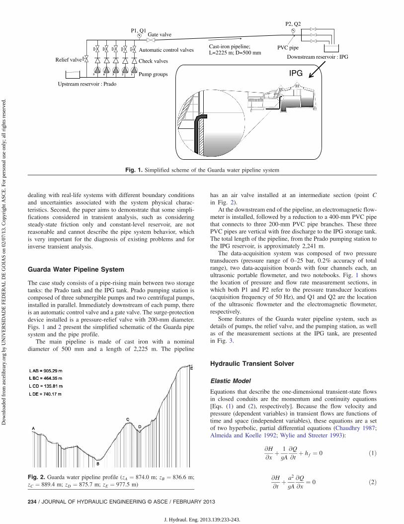
Equations that describe the one-dimensional transient-state flowsin closed conduits are the momentum and continuity equations[Eqs. (1) and (2), respectively]. Because the flow velocity andpressure (dependent variables) in transient flows are functions oftime and space (independent variables), these equations are a setof two hyperbolic, partial differential equations (Chaudhry 1987;Almeida and Koelle 1992; Wylie and Streeter 1993):

∂H∂x þ 1

gA∂Q∂t þ hf ¼ 0 ð1Þ

∂H∂t þ a2

gA∂Q∂x ¼ 0 ð2Þ

Upstream reservoir : Prado

Relief valve Check valves

Pump groups

Gate valve

Cast-iron pipeline;L=2225 m; D=500 mm

Downstream reservoir : IPG

5 4 3 2 1

P1, Q1P2, Q2

PVC pipeAutomatic control valves

IPG

Fig. 1. Simplified scheme of the Guarda water pipeline system

Fig. 2. Guarda water pipeline profile (zA ¼ 874.0 m; zB ¼ 836.6 m;zC ¼ 889.4 m; zD ¼ 875.7 m; zE ¼ 977.5 m)

234 / JOURNAL OF HYDRAULIC ENGINEERING © ASCE / FEBRUARY 2013

J. Hydraul. Eng. 2013.139:233-243.

Dow

nloa

ded

from

asc

elib

rary

.org

by

UN

IVE

RSI

DA

DE

FE

DE

RA

L D

E G

OIA

S on

02/

07/1

3. C

opyr

ight

ASC

E. F

or p

erso

nal u

se o

nly;

all

righ

ts r

eser

ved.

Fig. 3.Guarda water pipeline system: (a) Prado pumping station; (b) submergible pumps and relief valve; (c) centrifugal pumps; (d) pressure and flowrate measurement points in Prado pumping station; (e) ultrasonic flowmeter; (f) pressure transducer location in Prado pumping station; (g) electro-magnetic flowmeter and inlet PVC pipe in IPG reservoir; (h) crosspiece and PVC pipe branches in IPG reservoir; (i) pressure transducer in IPGreservoir; (j) free discharge outlet


J. Hydraul. Eng. 2013.139:233-243.

Dow

nloa

ded

from

asc

elib

rary

.org

by

UN

IVE

RSI

DA

DE

FE

DE

RA

L D

E G

OIA

S on

02/

07/1

3. C

opyr

ight

ASC

E. F

or p

erso

nal u

se o

nly;

all

righ

ts r

eser

ved.

where x = coordinate along the pipe axis; t = time; H = piezometrichead; Q = flow rate; A = pipe cross-sectional area; a = celerity (orelastic wave speed); g = gravity acceleration; and hf = head loss perunit length.

Considering an elastic behavior of the pipe wall, the wave speedfor monophasic fluids (i.e., liquids) can be estimated by (Wylie andStreeter 1993)

a ¼ffiffiffiffiffiffiffiffiffiffiffiffiffiffiffiffiffiffiffiffiffiffiffiffiffiffiffiffiffiffiffiffiffiffiffiffiffiffiffiffiffiffiffiffiffiffi

K2

ρ½1þ ψðD=eÞðK2=E0Þ�

sð3Þ

whereK2 = bulk modulus of elasticity of the fluid; ρ = mass densityof the fluid; E0 = Young’s modulus of elasticity of the pipe; D =pipe inner diameter; e = pipe-wall thickness; and ψ = dimensionlessparameter that depends on the elastic properties of the conduit(i.e., cross-section dimensions, pipe axial constraints, and Poisson’scoefficient). For gas-liquid mixtures, wave speed also dependson the gas initial concentration, pressure, and temperature(Chaudhry 1987).

The set of differential Eqs. (1) and (2) can be solved by themethod of characteristics, which allows the transformation of theseequations into a set of total differential equations valid along thecharacteristic lines, dx=dt ¼ �a

C�∶ dHdt

� agA

dQdt

� a · hf ¼ 0 ð4Þ

Using a rectangular computational grid (Fig. 4), these simplifiedequations can then be numerically solved by the following scheme:

C�∶ ðHi;t −Hi∓1;t−ΔtÞ �agA

ðQi;t −Qi∓1;t−ΔtÞ � aΔthf ¼ 0 ð5Þ

valid along Δx=Δt ¼ �a, respectively.To take into account unsteady friction effects, the friction losses,

hf , have been separated into two components

hf ¼ hfs þ hfu ¼fQjQj2gDA2

þ hfu ð6Þ

where hfs = head loss for steady-state conditions (expressed interms of square flow rate for turbulent flows); hfu = head lossfor unsteady-state conditions; and f = Darcy-Weisbach friction fac-tor calculated for turbulent and laminar flow by (Swamee 1993):

f ¼��

64

R

�8

þ 9.5

�ln

�ε

3.7Dþ 5.74

R0.9

�−�2; 500R

�6�−16�0.125

ð7Þ

where ε = pipe roughness; and R = Reynolds number.

With regard to the head loss for unsteady-state conditions,two one-dimensional models, developed by Vítkovský et al.(2000) and Vardy and Brown (2007), are considered. The unsteadyfriction model proposed by Brunone et al. (1991) and improvedby Vítkovský et al. (2000) is adequate for turbulent flows, isparameter-dependent, and is a function of both local and convec-tive accelerations. Two numerical schemes can be implemented.Brunone et al. (1991) proposed grid interpolations, whereas ageneral scheme was used by Vítkovský et al. (2000) without gridinterpolations. Brunone et al. (1991):

hfu ¼K3

gA

�∂Q∂t − a

∂Q∂x

�ð8Þ

Vítkovský et al. (2000):

hfu ¼k 0

gA

�∂Q∂t þ a · SGNðQÞ

�� ∂Q∂x��

ð9Þ

where K3 and k 0 = decay coefficient; and SGN = operator for thesign of the average flow rate.

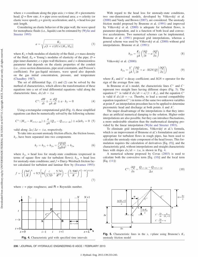
In Brunone et al.’s model, the characteristic lines Cþ and C−represent two straight lines having different slopes (Fig. 5). Theequation Cþ is valid if dx=dt ¼ a=ð1þ K3Þ, and the equation C–

is valid if dx=dt ¼ −a. Thereby, to lead a second compatibilityequation (equationCþ) in terms of the same two unknown variablesat point P, an interpolation procedure has to be applied to determinepiezometric head and discharge at both points A and A 0.

The major disadvantage of the interpolations is that they intro-duce an artificial numerical damping to the solution. Higher-orderinterpolations are also possible, but they can introduce fluctuations,a more undesirable situation than the mathematical damping pro-vided by the linear interpolation (Wylie and Streeter 1993).

To eliminate grid interpolations, Vítkovský et al.’s formula,which is an improvement of Brunone et al.’s formulation and moreappropriate for turbulent flows in rough pipes, has been used tocalculate the unsteady-state component of the head losses. This for-mulation requires the calculation of derivatives [Eq. (9)], and thecharacteristic grid, without interpolations and straight characteristiclines with slopes dx=dt ¼ �a, is shown in Fig. 4.

A numerical scheme proposed by Covas (2003) is used tocalculate both the convective term [Eq. (10)] and the local term[Eq. (11)]:

C�∶ ∂Q∂x ¼ Qi;t−Δt −Qi∓1;t−Δt

Δxð10Þ

1−i i 1+i

1 ...2 N... 1+N

A

P

B

+C −C

∆x = a·∆t

t

t ∆t−

t

x0=t

0= Lx x =

Fig. 4. Characteristic grid with specified time intervals

+C

−C

∆t

x∆

S

R A

A'

C B

P

( )a

K·x 13 +∆

a

K·x 3∆

a

xt

∆=∆ϕ

( )a

t

x:C

K

a

t

x:C

−=∆∆

+=

∆∆

−

+

13

Fig. 5. Characteristic lines in the x, t-plane using Brunone’s K3

unsteady friction model


J. Hydraul. Eng. 2013.139:233-243.

Dow

nloa

ded

from

asc

elib

rary

.org

by

UN

IVE

RSI

DA

DE

FE

DE

RA

L D

E G

OIA

S on

02/

07/1

3. C

opyr

ight

ASC

E. F

or p

erso

nal u

se o

nly;

all

righ

ts r

eser

ved.

C�∶ ∂Q∂t ¼ θQi;t −Qi;t−Δt

Δtþ ð1 − θÞQi∓1;t−Δt −Qi∓1;t−2Δt

Δtð11Þ

C�∶ SGNðQÞ ¼ SGNðQi∓1;t−ΔtÞ ð12Þwhere θ = relaxation coefficient. If θ ¼ 0, the flow time derivativebecomes explicit and unstable for certain conditions; if θ > 0,the numerical scheme is implicit and unconditionally stable. Tominimize computer storage and increase computational speed, theauthor have considered θ ¼ 1, and the same assumption has beenadopted in this study.

Zielke (1968) presented a formulation of the wall shear stress,which relates the unsteady friction component to the local accel-eration and a weighting function as follows:

hfuðtÞ ¼16νgD2

�∂V∂t �W

�ðtÞ ð13Þ

where ν = kinematic viscosity; V = average velocity; W = weight-ing function; and * denotes convolution, which indicates that theunsteady friction term is a convolution of past fluid accelerationswith a weighting function. Recently, Vardy and Brown (2007) for-mulated the weighting function as follows:

WðλÞ ¼X17i¼1

mie−niλ ð14Þ

where mi ¼ A�m�i ; ni ¼ B� þ n�i ; and λ ¼ 4νt=D2. The coeffi-

cientsm�i , n

�i , A

�, and B� are defined as in Vardy and Brown (2007).

Transients in Multipipe Systems: Generalized ElasticModel

The set of compatibility equations [Eq. (5)] can be solved numeri-cally by a general simplified linear form for the linear-elastic con-duit useful for complex multipipe systems

Cþ∶QPi ¼ CP − CaþHPi ð15Þ

C−∶QPi ¼ CN þ Ca−HPi ð16Þwhere i = pipe section; and CP, CN , Caþ, and Ca− = coefficientsthat depend on the numerical scheme used to describe steady-statefriction and the unsteady friction model adopted. These constants,in a generic form, can be defined as follows (Covas 2003; Soareset al. 2008):

CP ¼ Qi−1;t−Δt þ CaiHi−1;t−Δt þ C 0P1 þ C 00

P1

1þ C 0P2 þ C 00

P2ð17Þ

CN ¼ Qiþ1;t−Δt − CaiHiþ1;t−Δt þ C 0N1 þ C 00

N1

1þ C 0N2 þ C 00

N2

ð18Þ

Caþ ¼ Cai1þ C 0

P2 þ C 00P2

ð19Þ

Ca− ¼ Cai1þ C 0

N2 þ C 00N2

ð20Þ

where Cai ¼ gA=a. The coefficient superscripts ′ and ″ refer tothe steady-state friction and the unsteady friction components,respectively. The numerical description of each coefficient usedin this paper is presented in Table 1.

At any interior grid intersection point (point P at section i), thetwo compatibility equations [Eqs. (15) and (16)] are solved simul-taneously for the unknownsQPi andHPi. To complete the solution,appropriate boundary conditions have been introduced specifyingadditional equations at the ends of each pipe, which are presented inthe following sections.

Upstream Boundary Condition: Pump Trip Modeling

For the complete mathematical representation of a pump, the rela-tionships between discharge (Q), rotational speed (N), pumpinghead (H), and net torque (T) have to be specified, and they arecalled pump characteristics. Dimensionless parameters referringto the point of best efficiency (rated conditions) are used as a refer-ence and defined by the following variables, where the subscript Rdenotes rated conditions (Chaudhry 1987):

q ¼ QQR

; h ¼ HHR

; n ¼ NNR

; b ¼ TTR

ð21Þ

Considering additional boundary condition formulations,Chaudhry (1987) presents the basis for the calculations of the var-iables q, h, n, and b, in which an iterative procedure may be used.

By using the signs of these relationships, the pump operationmay be divided into eight operating zones and four quadrants,in terms of an angle ω ¼ tan−1ðn=qÞ, which includes normal pump-ing, reverse pumping, normal turbine, reverse turbine, and energydissipation (Chaudhry 1987; Ramos et al. 2005).

Pressure head and torque characteristic curves may be definedby the head and torque Suter parameters, Fh and Fb, respectively.

Table 1. Coefficients CP1, CP2, CN1, and CN2

Friction model Coefficients

Steady-state friction Frictionless C 0P1 ¼ C 0

P2 ¼ 0 C 0N1 ¼ C 0

N2 ¼ 0

First-order accuracy C 0P1 ¼ −RΔtjQi−1;t−ΔtjQi−1;t−Δt C 0

N1 ¼ −RΔtjQiþ1;t−ΔtjQiþ1;t−ΔtC 0P2 ¼ 0 C 0

N2 ¼ 0 R ¼ f=2DAUnsteady friction No unsteady friction C 00

P1 ¼ C 00P2 ¼ 0 C 00

N1 ¼ C 00N2 ¼ 0

Vítkovský et al. model C 00P1 ¼ k 0θQi;t−Δt − k 0ð1 − θÞðQi−1;t−Δt −Qi−1;t−2ΔtÞ− k 0SGNðQi−1;t−ΔtÞjQi;t−Δt −Qi−1;t−Δtj

C 00N1 ¼ k 0θQi;t−Δt − k 0ð1 − θÞðQiþ1;t−Δt −Qiþ1;t−2ΔtÞ− k 0SGNðQiþ1;t−ΔtÞjQi;t−Δt −Qiþ1;t−Δtj

C 00P2 ¼ C 00

N2 ¼ k 0θ

Vardy-Brown model C 00P1 ¼ C 00

N1 ¼ gAΔtð16ν=gD2ÞPkðe−nkð4υ=D2ÞΔtYk;j−1 − ðmk=AÞQi;j−1ÞC 00P2 ¼ C 00

N2 ¼ gAΔtð16ν=gD2ÞPkðmk=AÞ


J. Hydraul. Eng. 2013.139:233-243.

Dow

nloa

ded

from

asc

elib

rary

.org

by

UN

IVE

RSI

DA

DE

FE

DE

RA

L D

E G

OIA

S on

02/

07/1

3. C

opyr

ight

ASC

E. F

or p

erso

nal u

se o

nly;

all

righ

ts r

eser

ved.

These parameters may be plotted with ω for different values ofspecific speeds Ns (Fig. 6)

Fh ¼h

n2 þ q2; Fb ¼

bn2 þ q2

; Ns ¼NRQR

H3=4R

ð22Þ

In this study, the suction line of the pump is short compared withthe discharge line, and thus the water hammer waves in this line

may be neglected. Referring to Fig. 7, the following equationscan be written

HPi ¼ Hsuc þHP −ΔHPv ð23Þ

ΔHPv ¼ CvQPijQPij ð24Þ

QP ¼ QPi ¼ Cn þ CaiHPi ð25Þ

Cn ¼ QB − CaiHB − RΔtQBjQBj ð26Þwhere Hsuc = height of the liquid surface in the suction reservoirabove datum; HP = pumping head at the end of the time step;ΔHPv = head loss in the discharge valve; and Cv = head-losscoefficient in the valve.

Internal Condition: Check Valve

A check valve was installed downstream of the pump. Furtherexperimental analysis in the actual system is necessary to determinevalve coefficients related to the inertial effects of acceleratingand decelerating flow through the valve closing; however, this wasoutside of the scope of the current study. The check valve was de-scribed by an in-line valve with a steady-state orifice equation, andthe closure time was calibrated using observed data. A schematicrepresentation of the in-line valve is shown in Fig. 8. According toWylie and Streeter (1993), the following equations are defined for asingle check-valve modeling:

For positive flow → ðCA − CBÞ ≥ 0

QPi ¼ −CivðBA þ BBÞ þffiffiffiffiffiffiffiffiffiffiffiffiffiffiffiffiffiffiffiffiffiffiffiffiffiffiffiffiffiffiffiffiffiffiffiffiffiffiffiffiffiffiffiffiffiffiffiffiffiffiffiffiffiffiffiffiffiffiffiffiffiffiffiffiffiC2ivðBA þ BBÞ2 þ 2CivðCA − CBÞ

qð27Þ

For negative flow → ðCA − CBÞ < 0

QPi ¼ CivðBA þ BBÞ −ffiffiffiffiffiffiffiffiffiffiffiffiffiffiffiffiffiffiffiffiffiffiffiffiffiffiffiffiffiffiffiffiffiffiffiffiffiffiffiffiffiffiffiffiffiffiffiffiffiffiffiffiffiffiffiffiffiffiffiffiffiffiffiffiffiC2ivðBA þ BBÞ2 − 2CivðCA − CBÞ

qð28Þ

in which

CA ¼ HA þ BQA ð29Þ

CB ¼ HB − BQB ð30Þ

BA ¼ Bþ R 0jQAj ð31Þ

BB ¼ Bþ R 0jQBj ð32Þ

(a)

– 4

– 3

– 2

– 1

0

1

2

3

4

0 60 120 180 240 300 360

Ns = 0.46

Ns = 1.61

Ns = 2.78

Ns = 4.94

ω , in degreesPre

ssur

e (F

h)

(b) – 4

– 3

– 2

– 1

0

1

2

3

4

0 60 120 180 240 300 360

Ns = 0.46

Ns = 1.61

Ns = 2.78

Ns = 4.94

Tor

que

(Fb)

ω , in degrees

Fig. 6. Pump characteristic curves for different specific speeds:(a) pumping pressure head; (b) net torque

QP=QPii

C–

Datum

HPi

HP

Hsuc

∆HPv

Fig. 7. Pump with short suction line

B

C–C+

A

P P

Valve

ii – ∆ +ix ∆x

t – ∆ t

t

Fig. 8. Dynamic check valve modeled as an in-line valve


J. Hydraul. Eng. 2013.139:233-243.

Dow

nloa

ded

from

asc

elib

rary

.org

by

UN

IVE

RSI

DA

DE

FE

DE

RA

L D

E G

OIA

S on

02/

07/1

3. C

opyr

ight

ASC

E. F

or p

erso

nal u

se o

nly;

all

righ

ts r

eser

ved.

R 0 ¼ fΔx2gDA2

ð33Þ

B ¼ a=gA ð34Þ

Civ ¼ ðQ0τÞ2=ð2H0Þ ð35Þwhere τ = dimensionless valve-opening coefficient specified as afunction of time (τ ¼ 1 for fully opening; τ ¼ 0 for valve com-pletely closed); and H0 = steady-state drop in hydraulic grade lineacross the valve with a flow of Q0 when τ ¼ 1.

Downstream Boundary Condition: Variable-Level Tank

The last reach of the pipeline discharges to the atmosphere beforethe IPG storage tank. The final sections of the pipeline can bedescribed as variable-level tanks with free discharge to the atmos-phere and constant cross-sectional area. Similar consideration hasbeen presented in the literature by Di Santo et al. (2002) for risingmains with an air chamber. However, the authors have not takeninto account the unsteady friction losses. The following equationscan be written for the downstream boundary condition (Fig. 9):

QPi ¼ Cp − CaiHPi

Cp ¼ QA þ CaiHA − RΔtQAjQAjQd ¼ As

ffiffiffiffiffiffiffiffiffiffiffiffiffiffiffiffiffiffiffiffiffiffiffiffiffiffiffiffi2gðHPi −HTÞ

p9=; if HPi > HT ð36aÞ

QPi ¼ Cp − CaiHPi

Cp ¼ QA þ CaiHA − RΔtQAjQAjHPi ¼ Hs þ 0.5ðΔt=AsÞðQPi þQsÞQd ¼ 0

9>>=>>; if HPi ≤ HT ð36bÞ

where Qd = discharge into the downstream storage tank; As =cross-sectional area of the vertical tank; HT = elevation of thetank top; Hs = tank water level at the beginning of time step; andQs = flow rate at the beginning of time step.

Model Calibration

Pump-Motor Unit Inertia

The Prado pumping station is composed of five pumps installedin parallel. The field tests have been carried out by using onlypump 1, which is a submersible pump with the following nomi-nal parameters: pump discharge QR ¼ 300 m3=h, pumping headHR ¼ 105 m, power PR ¼ 110 kW, rotational speed NR ¼3;000 rpm, and efficiency ηR ¼ 0.78. Considering these nominal

values, the pump-motor inertia was calculated by the Thorleyand Faithfull (1992) formulation, in which I ¼ I1 þ I2, whereI1 = estimated inertia of the pump impeller and fluid; and I2 =inertia of the motor, given by

I1 ¼ 0.038

�PR

ðNR=1; 000Þ3�

0.96¼ 0.038

�110

33

�0.96

¼ 0.146 kg · m2 ð37Þ

I2 ¼ 0.0043

�PR

ðNR=1; 000Þ�

1.48¼ 0.0043

�110

3

�1.48

¼ 0.888 kg · m2 ð38ÞThe total inertia for the pump-motor unit was accordingly esti-

mated as I ¼ 1.034 kg · m2.

Check-Valve Closure

Because of the pump trip, the flow in the discharge line reducesrapidly to zero. To prevent reverse flow through the pump, thecheck valve installed downstream of the pump closes completely.This causes a stoppage of the flow with the corresponding pressurerise. In this study, the time of closure and the corresponding τversus t curve were calibrated. Fig. 10(a) depicts the calibratedcheck-valve closure, and Fig. 10(b) the respective flow rate atlocation Q1. After the pump trip, the check valve closes completelyin 1.77 s.

Wave-Speed Estimation

The second parameter to be determined and calibrated is the elasticwave speed, which can be estimated by theoretical formulas withthe modulus of elasticity provided by the manufacturer of the pipes

QPi i

C+

Datum

HPi HS

Water level at the end of time step

Water level at the beginning of time step

AS

Qd

HT

Fig. 9. Variable-level tank

0.0

0.2

0.4

0.6

0.8

1.0

0.0 0.5 1.0 1.5 2.0 2.5 3.0Time (s)

τ

(a)

-5

5

15

25

35

45

55

65

75

0 5 10 15 20

Flow

rat

e (L

/s)

Time (s)(b)

Fig. 10. (a) Calibrated check-valve closure; (b) the respective flow rateat location Q1


J. Hydraul. Eng. 2013.139:233-243.

Dow

nloa

ded

from

asc

elib

rary

.org

by

UN

IVE

RSI

DA

DE

FE

DE

RA

L D

E G

OIA

S on

02/

07/1

3. C

opyr

ight

ASC

E. F

or p

erso

nal u

se o

nly;

all

righ

ts r

eser

ved.

(Chaudhry 1987; Wylie and Streeter 1993). The celerity wasestimated as 1;130 m=s by using Eq. (3) and by considering thefollowing parameters for cast-iron pipes: pipe class K9 with elasticjoint, nominal diameter of 500 mm, external pipe diameter of532 mm; iron wall thickness e ¼ 9 mm, cement lining thicknessof 4.5 mm (i.e., total wall thickness of 13.5 mm), internal diameterof 505 mm; bulk modulus of elasticity of water K2 ¼ 2.19 GPa;mass density of water ρ ¼ 999 kg=m3; modulus of elasticity ofthe cast-iron pipe E0 ¼ 170 GPa; and Poisson’s coefficient of thecast-iron pipe equal to 0.25. Whereas the PVC section length isvery short when compared with the total length of the pipeline(16=2;241 ¼ 0.7%), its effect was taken into account. The wavespeed was estimated as 428 m=s considering the parameters forthe PVC pipes: nominal diameter of 200 mm, external pipe diam-eter of 222 mm; pipe-wall thickness e ¼ 8.9 mm, internal diameterof 204.2 mm; modulus of elasticity of the PVC pipe E0 ¼ 3.6 GPa;and Poisson’s coefficient equal to 0.46.

The wave speed of 1;130 m=s resulted in a computationalscheme with Δt ¼ 0.009823 s, Δx ¼ 11.1 m (202 pipe reachesbetween the pump and the downstream storage tank), and numberof Courant-Friedrichs-Lewy stability condition equal to 1, whichindicates that wave-speed adjustments/grid interpolations werenot used.

To analyze the pressure transients in the system, the followingtwo scenarios have been considered:1. Constant-level reservoir as the downstream boundary condi-

tion and calculating the head losses with and without theunsteady friction component—in this case, the IPG tank isdirectly linked to the pipeline.

2. Three variable-level tanks as the downstream boundary con-dition and considering unsteady friction effects—in this case,the three cells of the IPG storage tank are not linked to thepipeline, which discharges to the atmosphere (actual system).

All the field tests were carried out with the relief valve out ofservice (i.e., by closing the gate valve immediately at the down-stream end). In this way, such a protection device did not influencethe system behavior, which reduced the uncertainties related to the

different effects in pressure variations, such as the attenuation anddispersion attributable to unsteady friction and the pressure reliefattributable to the variable-level tanks.

Scenario 1: Constant-Level Reservoir as DownstreamBoundary Condition

In the first attempt to calibrate the transient solver, a constant-levelreservoir was assumed as the downstream end boundary condition.The transient event was simulated by using both the classic elasticmodel (with only a steady-state friction term) and the elastic modeltaking into account unsteady friction (UF) losses (Vítkovskýet al. 2000; Vardy and Brown 2007). The decay coefficient of theVítkovský model, k 0, was calibrated as 0.020. With regard tosteady-state friction losses, the actual pipe roughness, ε, was deter-mined on the basis of steady-state measurements of pressure headon both points P1 and P2. The head loss for steady-state condi-tions between points P1 and P2 was determined as 0.85 m,which is the difference between the piezometric heads in P1(874.00þ 104.35 ¼ 978.35 m) and P2 (977.50 m). The Darcy-Weisbach formulation has been used for head-loss calculations(L ¼ 2; 225 m; Q0 ¼ 72 L=s; D ¼ 0.505 m), in which the fric-tion factor was determined by the Swamee (1993) formulation[Eq. (7)]. The pipeline roughness, ε, was thus determined as2 mm. Comparisons between numerical results obtained by usingthe elastic transient solver with collected pressure data immediatelydownstream of the check valve (location P1) are presented inFig. 11. Transient pressures observed in the location P2 are pre-sented in Fig. 12, as well as the numerical results obtained bythe elastic model with a constant-level reservoir as the downstreamend boundary condition.

Initial minimum pressures are described accurately by the elas-tic models, but the attenuation of transient pressures cannot bedescribed by any of these models, even when unsteady frictionis incorporated in the transient solver. Compared with the classicelastic model (with quasi-steady friction), the elastic model withunsteady friction results in higher attenuation of pressure peaks

50

60

70

80

90

100

110

120

130

140

150

0 10 20 30 40 50 60

Pres

sure

hea

d (m

)

Time (s)

Classic elastic modelElastic model with UF (Vardy-Brown model)

Collected dataDetail Elastic model with UF (Vítkovský model)

Fig. 11. Observed pressure heads at location P1 versus numerical results of both classic elastic model and elastic model taking into account unsteadyfriction (constant-level reservoir as downstream end boundary condition) (Q0 ¼ 72 L=s; R ≈ 182;000)


J. Hydraul. Eng. 2013.139:233-243.

Dow

nloa

ded

from

asc

elib

rary

.org

by

UN

IVE

RSI

DA

DE

FE

DE

RA

L D

E G

OIA

S on

02/

07/1

3. C

opyr

ight

ASC

E. F

or p

erso

nal u

se o

nly;

all

righ

ts r

eser

ved.

and delays the transient pressure wave; however, the shape of thetransient pressure signal cannot be described (see the firstpressure peak, “Detail” in Fig. 11) and tends to get worse as thetransient propagates along the pipeline.

Possible phenomena, such as viscoelasticity and fluid-structureinteraction (pipe displacements), could occur in the PVC pipesbecause PVC is characterized by viscoelastic rheological behavior.Further discussion on the behavior of the transient pressure signal isneeded. First, the viscoelasticity effect smoothes down maximum/minimum transient pressures. This behavior is not verified in thetransient pressures observed, thus excluding the application of aviscoelastic transient solver. There is a delay in the pressure wave,which can be ascribed to the unsteady friction losses effect becausethe majority of the pipeline is composed of cast-iron pipes (2,225 mof cast-iron pipes and 16 m of PVC pipes). However, the unsteadyfriction models used in this paper are not able to reproduce thepressure relief observed in the first pressure peak (“Detail” inFig. 11), which propagates along time.

The key question is, thus, the physical justification for the pres-sure relief in observed maximum transient pressures (which isexactly the opposite behavior observed in the line-packing effect).When scrutinizing the transient pressures measured at location P2(Fig. 12), it is shown that a pressure relief occurs after the pressurewave has arrived at that location. In addition, the pressure headestablished in approximately 0.5 m after 150–160 s, which indi-cates that the water column in the PVC vertical pipe branches isapproximately 0.5 m—this is less than the vertical length of thefinal sections of the pipeline (three PVC pipe branches with a nomi-nal diameter of 200 mm and a vertical length of approximately3.0 m). It has been considered that, after the pump was switchedoff and while the pressure wave did not arrive at the downstreamend, water was still delivered to the downstream end storagetank. After the pressure wave has arrived at the downstream endof the pipeline, the discharge into the downstream storage tankapproaches zero, and the water column in the PVC pipe branchesoscillates. The pressure wave travels along the pipeline from thedownstream to upstream direction and passes by location P1 witha relief in the maximum pressure and behavior slightly distorted, asis shown in the observed pressure data (“Detail” in Fig. 11).

This is because there is a loss of water volume while the firstpressure wave does not reach the final section of the pipeline. Afterthe pressure wave reaches the downstream end, the water level in-side the three PVC pipes oscillates and then relieves the maximum/minimum pressures. The solution proposed in this study is thus to

model the water-level variation in the final section by variable-leveltanks with free discharge to the atmosphere. This solution does notrequire any characteristic grid modification during simulations be-cause the water column in the pipeline shrank and changing gridscan produce discontinuities in the numerical results.

Scenario 2: Variable-Level Tanks with Free Dischargeat the Downstream End

A second attempt to calibrate the hydraulic transient solver wascarried out by using three vertical tanks with variable levels andfree discharge into the IPG tank as the downstream end boundarycondition. The inner diameter of the three small vertical tanks wasequal to the inner diameter of the three PVC pipe branches in thefinal section of the pipeline: 204.2 mm. The elevation of the tanktop was assumed as the difference between the elevations of boththe IPG tank (977.50 m) and Prado pumping station (874.00 m)—that is, HT ¼ 103.5 m.

The head losses were calculated by using both the steady andunsteady components, in which Vítkovský et al.’s (2000) formu-lation has been used for the unsteady friction losses component.

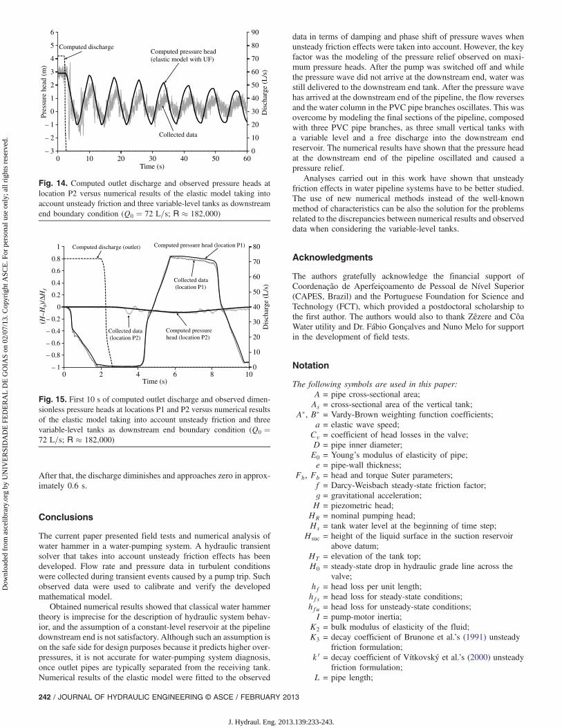
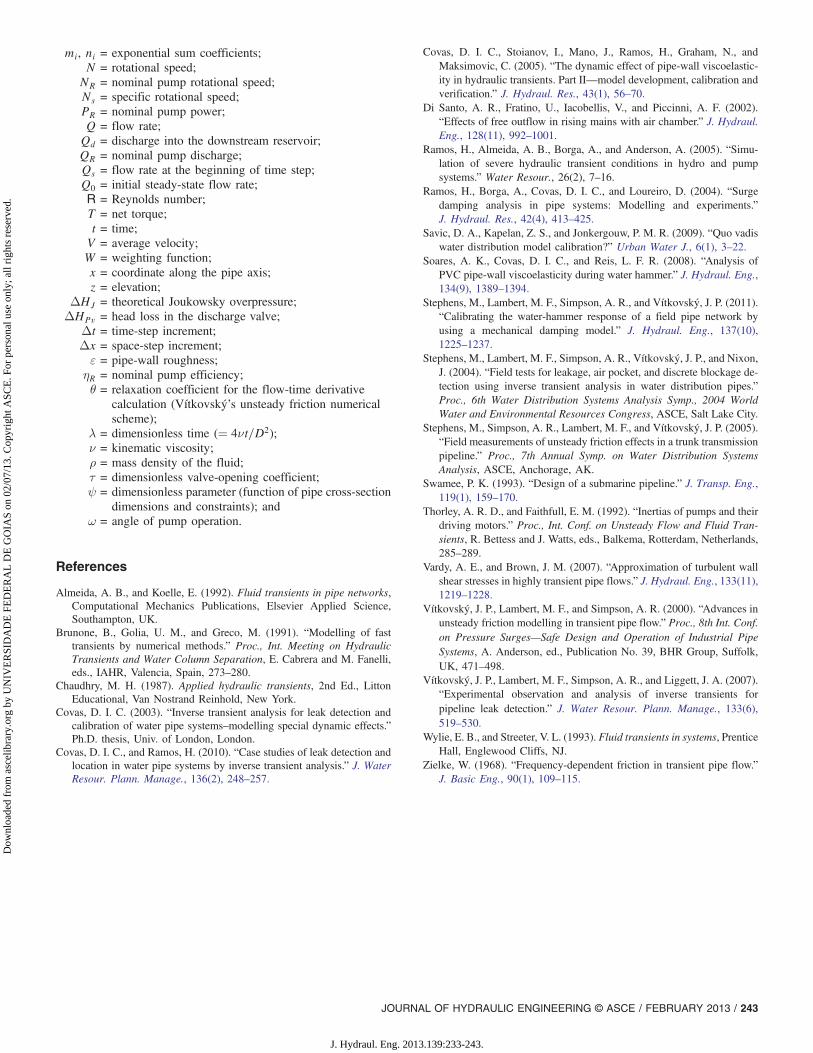
Fig. 13 shows the observed transient pressures for location P1and the numerical results obtained by using the elastic model withthe decay coefficient adjusted as k 0 ¼ 0.033. The numerical resultsfit extremely well with collected pressure data, and the modelcan describe transient pressure wave attenuation, dispersion, andshape. The pressure relief in the first maximum pressure peakcan be described by the model when the downstream end boundarycondition is defined as three variable-level tanks. However, somediscrepancy still remains, possibly attributable to the description ofthe boundary condition (rigid) neglecting the elasticity of bothwater and pipe wall. Transient pressures observed in location P2are presented in Fig. 14, as well as the numerical results obtainedby the elastic model considering UF and three variable-level tanksas the downstream end boundary condition. The adoption of var-iable-level tanks gives the pressure head variation observed at thedownstream end of the pipeline. Fig. 15 shows the dimensionlessobserved traces [ðH −H0Þ=ΔHJ where H0 = steady-state head;and ΔHJ = theoretical Joukowsky overpressure: ΔHJ ¼ aQ0=gA]at locations P1 and P2, as well as the computed pressure headsand discharge to the downstream end storage tank for the first10 s. Although the pressure head falls because of the pump trip,the discharge into the IPG tank remains at 72 L=s in the first 2 s.

-3

-2

-1

0

1

2

3

4

5

6

0 10 20 30 40 50 60

Pres

sure

hea

d (m

)

Time (s)

Elastic model with UF (Vítkovský model)

Collected data

Elastic model with UF (Vardy-Brown model)

Fig. 12. Observed pressure heads at location P2 versus numerical re-sults of both classic elastic model and elastic model taking into accountunsteady friction (constant-level reservoir as downstream end boundarycondition) (Q0 ¼ 72 L=s; R ≈ 182;000)

50

70

90

110

130

150

0 10 20 30 40 50 60

Pres

sure

hea

d (m

)

Time (s)

Numerical results

Collected data

Decay due to water level dropping in downstream tank

Decay due to unsteady friction

Fig. 13. Observed pressure heads at location P1 versus numericalresults of the elastic model taking into account unsteady friction andthree variable-level tanks as downstream end boundary condition(Q0 ¼ 72 L=s; R ≈ 182; 000)


J. Hydraul. Eng. 2013.139:233-243.

Dow

nloa

ded

from

asc

elib

rary

.org

by

UN

IVE

RSI

DA

DE

FE

DE

RA

L D

E G

OIA

S on

02/

07/1

3. C

opyr

ight

ASC

E. F

or p

erso

nal u

se o

nly;

all

righ

ts r

eser

ved.

After that, the discharge diminishes and approaches zero in approx-imately 0.6 s.

Conclusions

The current paper presented field tests and numerical analysis ofwater hammer in a water-pumping system. A hydraulic transientsolver that takes into account unsteady friction effects has beendeveloped. Flow rate and pressure data in turbulent conditionswere collected during transient events caused by a pump trip. Suchobserved data were used to calibrate and verify the developedmathematical model.

Obtained numerical results showed that classical water hammertheory is imprecise for the description of hydraulic system behav-ior, and the assumption of a constant-level reservoir at the pipelinedownstream end is not satisfactory. Although such an assumption ison the safe side for design purposes because it predicts higher over-pressures, it is not accurate for water-pumping system diagnosis,once outlet pipes are typically separated from the receiving tank.Numerical results of the elastic model were fitted to the observed

data in terms of damping and phase shift of pressure waves whenunsteady friction effects were taken into account. However, the keyfactor was the modeling of the pressure relief observed on maxi-mum pressure heads. After the pump was switched off and whilethe pressure wave did not arrive at the downstream end, water wasstill delivered to the downstream end tank. After the pressure wavehas arrived at the downstream end of the pipeline, the flow reversesand the water column in the PVC pipe branches oscillates. This wasovercome by modeling the final sections of the pipeline, composedwith three PVC pipe branches, as three small vertical tanks witha variable level and a free discharge into the downstream endreservoir. The numerical results have shown that the pressure headat the downstream end of the pipeline oscillated and caused apressure relief.

Analyses carried out in this work have shown that unsteadyfriction effects in water pipeline systems have to be better studied.The use of new numerical methods instead of the well-knownmethod of characteristics can be also the solution for the problemsrelated to the discrepancies between numerical results and observeddata when considering the variable-level tanks.

Acknowledgments

The authors gratefully acknowledge the financial support ofCoordenação de Aperfeiçoamento de Pessoal de Nível Superior(CAPES, Brazil) and the Portuguese Foundation for Science andTechnology (FCT), which provided a postdoctoral scholarship tothe first author. The authors would also to thank Zêzere and CôaWater utility and Dr. Fábio Gonçalves and Nuno Melo for supportin the development of field tests.

Notation

The following symbols are used in this paper:A = pipe cross-sectional area;As = cross-sectional area of the vertical tank;

A�, B� = Vardy-Brown weighting function coefficients;a = elastic wave speed;

Cv = coefficient of head losses in the valve;D = pipe inner diameter;E0 = Young’s modulus of elasticity of pipe;e = pipe-wall thickness;

Fh, Fb = head and torque Suter parameters;f = Darcy-Weisbach steady-state friction factor;g = gravitational acceleration;H = piezometric head;

HR = nominal pumping head;Hs = tank water level at the beginning of time step;

Hsuc = height of the liquid surface in the suction reservoirabove datum;

HT = elevation of the tank top;H0 = steady-state drop in hydraulic grade line across the

valve;hf = head loss per unit length;hfs = head loss for steady-state conditions;hfu = head loss for unsteady-state conditions;I = pump-motor inertia;

K2 = bulk modulus of elasticity of the fluid;K3 = decay coefficient of Brunone et al.’s (1991) unsteady

friction formulation;k 0 = decay coefficient of Vítkovský et al.’s (2000) unsteady

friction formulation;L = pipe length;

0

10

20

30

40

50

60

70

80

90

– 3

– 2

– 1

0

1

2

3

4

5

6

0 10 20 30 40 50 60

Dis

char

ge (

L/s

)

Pres

sure

hea

d (m

)

Time (s)

Computed pressure head(elastic model with UF)

Collected data

Computed discharge

Fig. 14. Computed outlet discharge and observed pressure heads atlocation P2 versus numerical results of the elastic model taking intoaccount unsteady friction and three variable-level tanks as downstreamend boundary condition (Q0 ¼ 72 L=s; R ≈ 182;000)

0

10

20

30

40

50

60

70

80

– 1

– 0.8

– 0.6

– 0.4

– 0.2

0

0.2

0.4

0.6

0.8

1

0 2 4 6 8 10

Dis

char

ge (

L/s

)

(H –

H0)

/∆H

J

Time (s)

Collected data(location P1)

Computed pressure head (location P1)Computed discharge (outlet)

Collected data(location P2)

Computed pressurehead (location P2)

Fig. 15. First 10 s of computed outlet discharge and observed dimen-sionless pressure heads at locations P1 and P2 versus numerical resultsof the elastic model taking into account unsteady friction and threevariable-level tanks as downstream end boundary condition (Q0 ¼72 L=s; R ≈ 182;000)


J. Hydraul. Eng. 2013.139:233-243.

Dow

nloa

ded

from

asc

elib

rary

.org

by

UN

IVE

RSI

DA

DE

FE

DE

RA

L D

E G

OIA

S on

02/

07/1

3. C

opyr

ight

ASC

E. F

or p

erso

nal u

se o

nly;

all

righ

ts r

eser

ved.

mi, ni = exponential sum coefficients;N = rotational speed;

NR = nominal pump rotational speed;Ns = specific rotational speed;PR = nominal pump power;Q = flow rate;Qd = discharge into the downstream reservoir;QR = nominal pump discharge;Qs = flow rate at the beginning of time step;Q0 = initial steady-state flow rate;R = Reynolds number;T = net torque;t = time;V = average velocity;W = weighting function;x = coordinate along the pipe axis;z = elevation;

ΔHJ = theoretical Joukowsky overpressure;ΔHPv = head loss in the discharge valve;

Δt = time-step increment;Δx = space-step increment;ε = pipe-wall roughness;

ηR = nominal pump efficiency;θ = relaxation coefficient for the flow-time derivative

calculation (Vítkovský’s unsteady friction numericalscheme);

λ = dimensionless time (¼ 4νt=D2);ν = kinematic viscosity;ρ = mass density of the fluid;τ = dimensionless valve-opening coefficient;ψ = dimensionless parameter (function of pipe cross-section

dimensions and constraints); andω = angle of pump operation.

References

Almeida, A. B., and Koelle, E. (1992). Fluid transients in pipe networks,Computational Mechanics Publications, Elsevier Applied Science,Southampton, UK.

Brunone, B., Golia, U. M., and Greco, M. (1991). “Modelling of fasttransients by numerical methods.” Proc., Int. Meeting on HydraulicTransients and Water Column Separation, E. Cabrera and M. Fanelli,eds., IAHR, Valencia, Spain, 273–280.

Chaudhry, M. H. (1987). Applied hydraulic transients, 2nd Ed., LittonEducational, Van Nostrand Reinhold, New York.

Covas, D. I. C. (2003). “Inverse transient analysis for leak detection andcalibration of water pipe systems–modelling special dynamic effects.”Ph.D. thesis, Univ. of London, London.

Covas, D. I. C., and Ramos, H. (2010). “Case studies of leak detection andlocation in water pipe systems by inverse transient analysis.” J. WaterResour. Plann. Manage., 136(2), 248–257.

Covas, D. I. C., Stoianov, I., Mano, J., Ramos, H., Graham, N., andMaksimovic, C. (2005). “The dynamic effect of pipe-wall viscoelastic-ity in hydraulic transients. Part II—model development, calibration andverification.” J. Hydraul. Res., 43(1), 56–70.

Di Santo, A. R., Fratino, U., Iacobellis, V., and Piccinni, A. F. (2002).“Effects of free outflow in rising mains with air chamber.” J. Hydraul.Eng., 128(11), 992–1001.

Ramos, H., Almeida, A. B., Borga, A., and Anderson, A. (2005). “Simu-lation of severe hydraulic transient conditions in hydro and pumpsystems.” Water Resour., 26(2), 7–16.

Ramos, H., Borga, A., Covas, D. I. C., and Loureiro, D. (2004). “Surgedamping analysis in pipe systems: Modelling and experiments.”J. Hydraul. Res., 42(4), 413–425.

Savic, D. A., Kapelan, Z. S., and Jonkergouw, P. M. R. (2009). “Quo vadiswater distribution model calibration?” Urban Water J., 6(1), 3–22.

Soares, A. K., Covas, D. I. C., and Reis, L. F. R. (2008). “Analysis ofPVC pipe-wall viscoelasticity during water hammer.” J. Hydraul. Eng.,134(9), 1389–1394.

Stephens, M., Lambert, M. F., Simpson, A. R., and Vítkovský, J. P. (2011).“Calibrating the water-hammer response of a field pipe network byusing a mechanical damping model.” J. Hydraul. Eng., 137(10),1225–1237.

Stephens, M., Lambert, M. F., Simpson, A. R., Vítkovský, J. P., and Nixon,J. (2004). “Field tests for leakage, air pocket, and discrete blockage de-tection using inverse transient analysis in water distribution pipes.”Proc., 6th Water Distribution Systems Analysis Symp., 2004 WorldWater and Environmental Resources Congress, ASCE, Salt Lake City.

Stephens, M., Simpson, A. R., Lambert, M. F., and Vítkovský, J. P. (2005).“Field measurements of unsteady friction effects in a trunk transmissionpipeline.” Proc., 7th Annual Symp. on Water Distribution SystemsAnalysis, ASCE, Anchorage, AK.

Swamee, P. K. (1993). “Design of a submarine pipeline.” J. Transp. Eng.,119(1), 159–170.

Thorley, A. R. D., and Faithfull, E. M. (1992). “Inertias of pumps and theirdriving motors.” Proc., Int. Conf. on Unsteady Flow and Fluid Tran-sients, R. Bettess and J. Watts, eds., Balkema, Rotterdam, Netherlands,285–289.

Vardy, A. E., and Brown, J. M. (2007). “Approximation of turbulent wallshear stresses in highly transient pipe flows.” J. Hydraul. Eng., 133(11),1219–1228.

Vítkovský, J. P., Lambert, M. F., and Simpson, A. R. (2000). “Advances inunsteady friction modelling in transient pipe flow.” Proc., 8th Int. Conf.on Pressure Surges—Safe Design and Operation of Industrial PipeSystems, A. Anderson, ed., Publication No. 39, BHR Group, Suffolk,UK, 471–498.

Vítkovský, J. P., Lambert, M. F., Simpson, A. R., and Liggett, J. A. (2007).“Experimental observation and analysis of inverse transients forpipeline leak detection.” J. Water Resour. Plann. Manage., 133(6),519–530.

Wylie, E. B., and Streeter, V. L. (1993). Fluid transients in systems, PrenticeHall, Englewood Cliffs, NJ.

Zielke, W. (1968). “Frequency-dependent friction in transient pipe flow.”J. Basic Eng., 90(1), 109–115.


J. Hydraul. Eng. 2013.139:233-243.

Dow

nloa

ded

from

asc

elib

rary

.org

by

UN

IVE

RSI

DA

DE

FE

DE

RA

L D

E G

OIA

S on

02/

07/1

3. C

opyr

ight

ASC

E. F

or p

erso

nal u

se o

nly;

all

righ

ts r

eser

ved.

http://dx.doi.org/10.1061/(ASCE)0733-9496(2010)136:2(248)


http://dx.doi.org/10.1080/00221680509500111



http://dx.doi.org/10.1080/00221686.2004.9641209

http://dx.doi.org/10.1080/15730620802613380





http://dx.doi.org/10.1061/(ASCE)0733-947X(1993)119:1(159)

http://dx.doi.org/10.1061/(ASCE)0733-947X(1993)119:1(159)





http://dx.doi.org/10.1115/1.3605049

Damping Analysis of Hydraulic Transients in Pump-Rising...

Documents

Transcript of Damping Analysis of Hydraulic Transients in Pump-Rising...