Rakenteiden Mekaniikka (Journal of Structural Mechanics)Vol. 48, No 2, 2015, pp. 99 – 114rmseura.tkk.fi/rmlehti/c©The authors 2015.

Open access under CC BY-SA 4.0 license.

Damage-viscoplastic model based on the Hoek-Browncriterion for numerical modeling of rock fracture

Timo Saksala

Summary. This article presents a phenomenological damage-viscoplastic model based on theempirical Hoek-Brown criterion for numerical modeling of rock fracture. The viscoplastic part ofthe model is formulated in the spirit of the consistency model by Wang (1997). Isotropic damagemodel with separate damage variables in tension and compression is employed to describe thestiffness and strength degradation. The model is implemented with the FE method using theconstant strain triangle elements. The equations of motion are solved with the explicit timemarching scheme. In the numerical examples, after demonstrating the model response at thematerial point level, confined compression and uniaxial tension tests on rock are simulated asquasi-static problems. Moreover, the dynamic three-point bending of a notched semicirculardisc test is simulated in order to demonstrate the model predictions under dynamic loadingconditions.

Key words: Hoek-Brown criterion, viscoplastic consistency model, isotropic damage, finite ele-

ment method, rock fracture

Received 17 February 2015. Accepted 23 June 2015. Published online 20 November 2015

Introduction

Numerical modeling of rock fracture is an active area of research in the field of compu-tational mechanics due to its importance in failure analyses of underground rock struc-tures and rock breakage industry. The major challenges therein are related to numericalmodeling of crack propagation and numerical description of rock micro-structure. Manynumerical models, based on the finite element method and the discrete element method,have been developed during the last decades for the simulation of rock fracture. For areview article on numerical methods in rock mechanics, see [1].

In the present paper the continuum approach based on the finite element method ischosen due to its computational efficiency and maturity as a numerical method. It will beseen that despite its underlying principle of treating materials as a continuous medium,it can be successfully, in the engineering sense, employed in modeling crack propagationunder dynamic and quasi-static loading conditions even in brittle materials such as rock.For this end, a constitutive model based on a combination of the isotropic damage concept[3] and viscoplastic consistency model by Wang et al. [2] is developed.

The damage part of the model with separate damage variables in tension and com-pression describes the stiffness and strength degradation of the material under loading.

99

The viscoplastic part of the model, which governs the inelastic strain development andthe strain-rate dependency, is based on the Hoek-Brown failure criterion for rocks [4]. Thechoice of this criteria is justified based on the test data and implementation economy andsimplicity grounds. The damage and viscoplastic parts are combined with the effectivestress space formulation [5]. The model is implemented in explicit dynamics FE setting.

The model predictions are demonstrated first at the material point level simulationusing a single constant strain triangle element. Then the model is tested at the laboratorysample level in 2D simulations. First, the confined compression and uniaxial tension testson rock are simulated. Second, dynamic three-point bending test of a notched semicircularrock sample is simulated as a transient problem involving contact.

Theory of the material model for rock

The theory of the model is presented here. First, the viscoplastic part of the modelbased on the viscoplastic consistency approach is formulated. Then, the isotropic damagemodel is developed for present purposes. The model components are combined with theeffective stress space approach. The details of stress integration are also presented forthe convenience of the reader. Third, the explicit time integration method for solving theequations of motion is presented. Finally, the statistical modeling of rock strengths basedon the Weibull distribution is briefly sketched.

Viscoplasticity part of the model

Classical viscoplasticity formulations, such as the Perzyna model, do not utilize the con-sistency condition. Consequently, a trial stress state violating the yield criterion is notreturned to the yield surface. However, Wang et al. [2] presented a so-called viscoplasticconsistency model which utilizes the consisteny condition and thus recasts the viscoplas-ticity theory into the classical computational plasticity format. The major difference ofthis formulation to the classical plasticity models is the dependence of the yield functionon the rate of the internal variables. The main ingredients of such a model are

fvp = f(σ, κ, κ), (1)

εvp = λ∂gvp

∂σ, κ = λk(σ, κ), (2)

fvp ≤ 0, λ ≥ 0, λfvp = 0, (3)

where σ is the stress tensor, gvp is the viscoplastic potential, fvp is the dynamic yieldfunction, κ, κ are the internal variable and its rate, respectively, λ is the viscoplasticincrement and k(σ, κ) is a function relating the rates of κ and λ. Equation (2) expressesthe non-associated flow rule (the associated case is obtained by gvp = fvp) while Equation(3) states the Kuhn-Tucker loading-unloading conditions. Finally, as rocks are brittle ma-terials, the present model can be formulated under the assumption of small deformations(and rigid body rotations). Therefore, the decomposition of the total strain rate intoelastic and viscoplastic parts

ε = εe + εvp (4)

is performed here as in the rate independent plasticity.The consistency condition becomes

fvp(σ, κ, κ) =∂fvp

∂σ: σ +

∂fvp

∂κκ+

∂fvp

∂κκ. (5)

100

This can be rewritten, using Equation (2), as

∂fvp

∂σ: σ − hλ− sλ = 0, (6)

where

h = −∂fvp

∂κk(σ, κ)− ∂fvp

∂κk(σ, κ), (7)

s = −∂fvp

∂κk(σ, κ) (8)

are the generalized plastic and viscoplastic moduli, respectively. The consistency condi-tion is now a first order differential equation for λ. However, in the algorithmic treatmentof the model, the rate of the internal variable is eliminated by approximation κ ≈ k∆λ/∆t.Thereby, the standard methods of computational rate-independent plasticity can be ap-plied in the numerical implementation of the model. This issue will be treated in detaillater in this paper.

As for the selection of the yield function (or criterion), the work by Colmenares andZoback [7] is taken as a starting point. They evaluate statistically seven intact rock failurecriteria against polyaxial data of five different rocks. The criteria they study are the Mohr-Coulomb, Hoek-Brown, Drucker-Prager, Modified Lade, Modified Wiebols and Cook, andempirical Mogi 1961 and 1971 criteria. According to their findings, the polyaxial ModifiedWielbols and Cook and Modified Lade criteria fit well most of the test data, especiallyfor the rocks with a high intermediate stress (σ2) dependency (Dunham Dolomite andSolnhofen limestone). However, the Mohr-Coulomb and Hoek-Brown criteria, which ne-glect the influence of the intermediate stress, fit the data equally well (or even better)than the more complex criteria with rocks that do not show strong σ2-dependency (Shi-rahama sandstone and Yuubari shale). Therefore, the polyaxial criteria may be droppedfrom the list of candidates due to their complexity and questionable benefit with respectto accuracy for some rocks. The final selection is to be done between the Mohr-Coulomband te Hoek-Brown criteria.

The Hoek-Brown (HB) criterion, developed originally by Hoek and Brown [4], is a non-linear, allegedly empirical strength criterion developed primarily from the test data forapplication to excavation design. This criterion better matches the experimental data ofsome rocks under quasi-static compression, especially in the highly confined region, thanthe widely used Mohr-Coulomb criterion (this follows from the fact that MC criterion islinear but the experimental strength envelopes of many rocks are nonlinear). The HBcriterion is superior to MC criterion under dynamic loading conditions as well [6]. Forthese reasons, it is chosen as a yield function in this paper. In its generalized form fordifferent rock types and masses the criterion reads [8]

σ1 = σ3 + σc

(mσ3

σc

+ s

)a, (9)

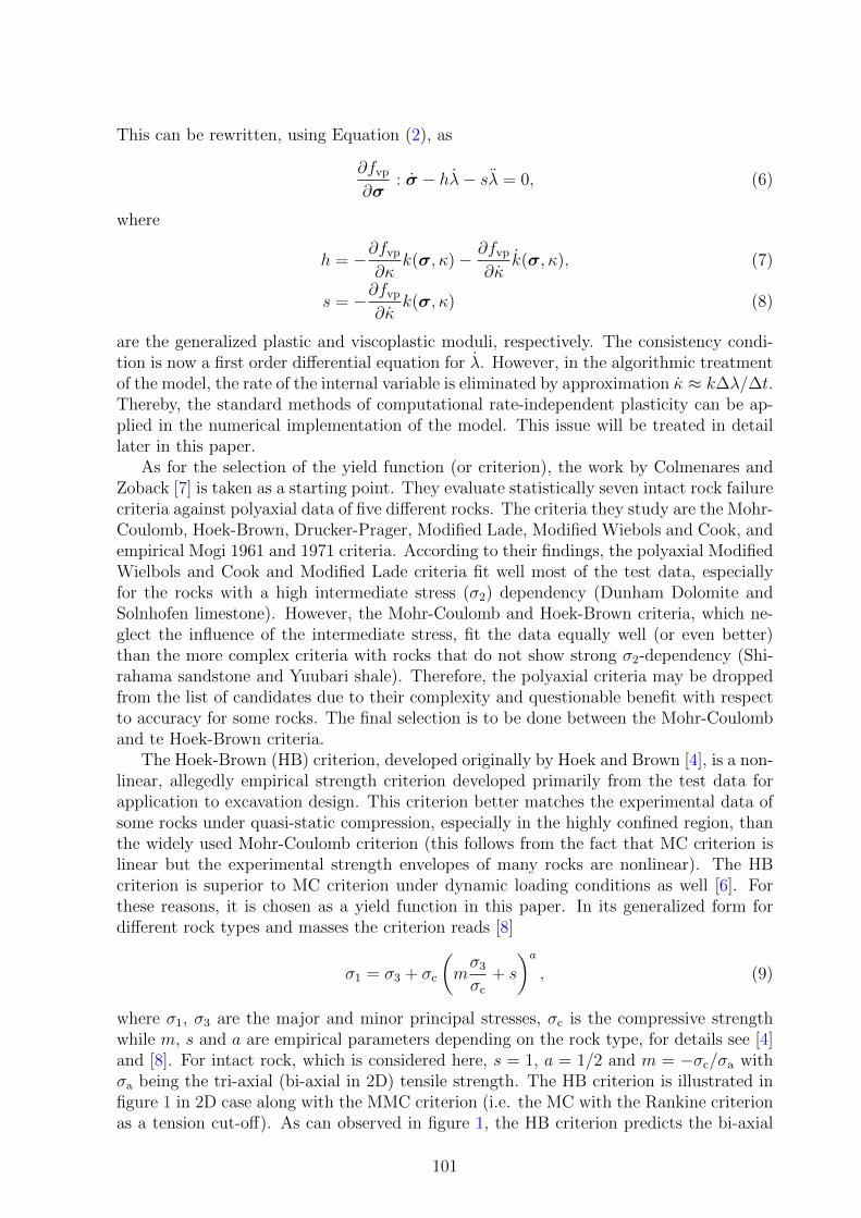
where σ1, σ3 are the major and minor principal stresses, σc is the compressive strengthwhile m, s and a are empirical parameters depending on the rock type, for details see [4]and [8]. For intact rock, which is considered here, s = 1, a = 1/2 and m = −σc/σa withσa being the tri-axial (bi-axial in 2D) tensile strength. The HB criterion is illustrated infigure 1 in 2D case along with the MMC criterion (i.e. the MC with the Rankine criterionas a tension cut-off). As can observed in figure 1, the HB criterion predicts the bi-axial

101

Figure 1. Hoek-Brown and modified Mohr-Coulomb criterions projected on the σ1 − σ3 plane.

tensile strength slightly higher than the uni-axial one. This feature may be questioned onphysical grounds but such a discussion is beyond the scope of the present paper.

For present purposes, the viscoplastic yield function based on the HB criterion andthe linear rate-dependent hardening softening rules for tensile and compressive strengthsare written as

fHB(σ, λ, λ) = (σ1 − σ3)2 + σc(λ, λ)2

(σ1

σt(λ, λ)− 1

), (10)

σt = σt0 + htλ+ stλ, (11)

σc = σc0 + hcλ+ scλ. (12)

In writing the yield function in (10), function k relating the internal variable and vis-coplastic increment is taken unity for simplicity, i.e. k(σ, κ) ≡ 1, giving κ = λ. Moreover,the model behavior is assumed to be perfectly viscoplastic, i.e. hence forward ht = 0 andhc = 0. This setting means that the strength (and stiffness) degradation or softening isgoverned by the damage part of model while the viscoplastic part incorporates the rate-dependency and indicates the stress states leading to damage. As for the viscosity moduli,st, sc, they are assumed to be constants for simplicity and due to the lack of experimentaldata. Finally, associated plasticity is assumed here for simplicity, i.e. gHB = fHB.

A note on implementation economy related to the HB and MMC models is in orderhere. Namely, a model based on the HB criterion represents - more or less successfully -the asymmetric behavior of rock in tension and compression with a single surface whereasthe MC criterion needs a tensile cut-off to mend its poor tensile strength prediction.This is a computational advantage as no corner plasticity situations appear in the nu-merical implementation of the model. The MMC criterion, in contrast to HB criterion,requires corner plasticity treatment at the non-smooth transition from the MC flow tothe Rankine flow and vice versa, see figure 1. On the other hand, the MMC criterionis (piecewise) linear while the HB criterion is nonlinear needing thus an iterative returnmapping method. Moreover, the computational efficiency of MMC criterion is consider-ably improved by Clausen et al. [9] (perfectly plastic case) and Saksala [10] (extensionto linear softening/hardening). Still, from the simplicity’s point of view (Occam’s Ra-zor could be invoked here), a criterion that matches the uniaxial tensile and compressive

102

strengths of rock with a single mathematical expression is preferable to those requiringtwo expressions.

Before proceeding to the damage part of the model, is also reminded that the viscosityis incorporated in the present approach in order to regulate the ill-posed problem ofclassical strain softening continua (plasticity), i.e. viscosity provides a localization limiter.Moreover, the loading rate sensitivity can be nicely accommodated through viscosity.Hence, the viscosity moduli above do not represent any material property of rock - theyare numerical parameters of the mathematical model.

Damage part of the model

The damage part of the model is formulated within the well established isotropic damagetheory (see e.g. [3]) with separate scalar damage variables in tension and compression.In the present formulation, damage evolution is driven by the viscoplastic strain. Conse-quently, no damage loading function is needed. Thus, specification is needed only for thedamage evolution laws and the equivalent viscoplastic strains that drive the damaging.Typical exponential damage evolution laws along with the equivalent viscoplastic strainsin tension and compression, εvp

eqvtand εvpeqvc, are employed here as

ωt = At(1− exp(βtεvpeqvt)), (13)

ωc = Ac(σconf)(1− exp(βc(σconf)εvpeqvc)), (14)

εvpeqvt =

√√√√ 3∑i=1

〈εvpi 〉2+, (15)

εvpeqvc =

√23εvp

dev : εvpdev. (16)

The positive part operator 〈x〉+ = max(x, 0) has been used on the rates of the viscoplasticprincipal strain components εvp

i in (15). Moreover, εvpdev is the deviatoric viscoplastic strain

and parameters At, βt in (13) and (14) control the maximum value of damage and theinitial slope of damage evolution, respectively. In compression, parameters Ac, βc arefunctions of confining pressure σconf which is the lateral pressure in the triaxial compressiontest. In numerical simulations, it can be calculated as σconf = 1

2(σ1 + σ2) if σ1 < 0

(otherwise it is zero). The effect of confining pressure in the triaxial compression testdepends on the rock type. This dependence is specified here for the Carrara marblefollowing Fang and Harrison [11] and Saksala and Ibrahimbegovic [12]. Accordingly,these parameters depend on the confining pressure and the fracture energies as follows

Ac(σconf) = Ac0 exp(−ndσconf), (17)

βc(σconf) = βc0 exp(−ndσconf), (18)

βc0 =σc0he

GIIc

, βt =σt0he

GIc

, (19)

where nd is an experimental parameter depending on the rock type and he is a character-istic length. In the FE context it is the element side length. This choice of making theamount of dissipation dependent on the mesh is justified by the fact that even thoughviscoplasticity provides a localization limiter for the ill-posed problem of classical soften-ing continuum, the amount of dissipation needs to be tied to a material parameter which

103

in the present case are the fracture energies GIc and GIIc. The model thus defined pre-dict the correct amount of dissipation in uniaxial tension and compression irrespective ofthe mesh refinement. Moreover, as a result of equation (18), the maximum value of thecompressive damage of the rock sample in confined compression decreases (exponentially)as confinement increases. This in turn means that the residual strength of of the sampleincreases as a function of confining pressure. Therefore, the model is able to predict theconfining pressure dependent brittle-to-ductile transition exhibited by compact carbonaterocks such as marble and limestone.

Finally, the nominal-effective stress relation addressing the unilateral conditions re-lated to microcrack closure and opening as

σ = (1− ωt)σ+ + (1− ωc)σ−, (20)

where the positive-negative part split of the principal effective stress σ has been usedwith σ+ = max(σ, 0) and σ− = min(σ, 0).

Solving the stress for a finite element

The solution method for the stress at an integration point of a finite element is presentedin this subsection for the convenience of the reader. The combination of the viscoplasticand damage parts of the model is based on the effective stress space formulation since itallows for a separation of the (visco)plasticity and damage computations and facilitatesthus the implementation.

The stress return mapping is based on the cutting plane algorithm described e.g. inSimo and Hughes [13]. At the end of a time step, condition fHB(σt+∆t, λt+∆t, λt+∆t) = 0must be satisfied. Now, following assumptions are used to eliminate the internal variableand its rate at the end of the time step

λt+∆t = λt + ∆λt+∆t, λt+∆t = ∆λt+∆t/∆t. (21)

With these relations, the condition to be fulfilled becomes fHB(σt+∆t,∆λt+∆t) = 0. Thiscan be expanded with the first term of Taylor series to obtain the algorithmic incrementδλ (dropping the subscript t+ ∆t and the dependency on the stress for brevity) as

fHB(∆λ) + ∂∆λfHB(∆λ)δλ = 0⇔ δλ = G−1fHB(∆λ) (22)

with G = −∂∆λfHB(∆λ) =∂fHB

∂σ: E :

∂fHB

∂σ− q · s, (23)

q = [−σ2c

σt

σ1, 2σc

(σ1

σt

− 1

)]T, (24)

s =1

∆t[st, sc]

T. (25)

As the HB criterion is expressed in terms of principal stresses, the stress return mappingis performed in the principal stress space. Next, the main steps of the return mapping uti-lizing the standard elastic predictor-(visco)plastic corrector split are presented assuming

104

the plastic case is realized, i.e. f trialHB = fHB(σtrial, λt, λt) > 0 with σtrial = E : (εt+∆t−εvp

t ):

δλn =fnHB

∂fnHB

∂σn: E :

∂fnHB

∂σn− qn · s

, (26)

∆λn+1 = ∆λn + δλn, (27)

εvpn+1 = εvp

n + δλn∂fnHB

∂σn

, (28)

σn+1 = σn + δλnE :∂fnHB

∂σn

, (29)

σt,n+1 = σt0,n + st∆λn+1

∆t, (30)

σc,n+1 = σc0,n + sc∆λn+1

∆t. (31)

These steps are repeated until fnHB < TOL where TOL is the convergence tolerance.After the stress update is performed, the equivalent viscoplastic strains and the damagevariables are updated based on Equations (13) - (16). Finally, the nominal stress iscalculated by Equation (20). The nominal stress is then used for calculation of the internalforce vector at the integration point of a finite element as f eint =

∫dV

BTσedV with B beingthe kinematic matrix.

Solving the equations of motion

The material model for rock presented above is implemented with the FE method (spatialdiscretization). As the aim is to simulate transient dynamic problems involving impactand stress wave propagation, in addition to quasi-static tests, the equations of motionare discretized explicitly in time. The mofidied Euler method is chosen for this end.Accordingly, the response (velocity and displacement) of the system is predicted as follows

ut = M−1(f text − f tint), (32)

ut+∆t = ut + ∆tut, (33)

ut+∆t = ut + ∆tut+∆t, (34)

where M is the lumped mass matrix, and u, u, u are the displacement, velocity andacceleration vector respectively.

Statistical description of rock strength

Rock is a heterogeneous material consisting of different minerals with different materialproperties, orientation and size. This heterogeneity leads to the statistical nature ofrock and is the major feature influencing rock fracture processes through the formation,extension and coalescence of microcracks. Therefore, heterogeneity should be taken intoaccount in numerical modeling aiming at realistic prediction, see e.g. [14]. Generally,the numerical description of rock microstructure depends, at least to some extent, on thechosen modeling approach.

In the present continuum approach based on finite elements, the simplest methodto account for rock strength heterogeneity is to assume the strength properties to bestatistically distributed element-wise. Here the method originally presented by Tang [15]

105

is followed. Accordingly, the uniaxial compressive strengh of rock is assumed to be Weibulldistributed. The three-parameter Weibull propability distribution function reads

Pr(x) = 1− exp

(−x− xu

x0

)mw

, (35)

where, in the mechanics context, the shape parameter mw is interpreted as the homogene-ity index, the scale parameter x0 is taken as the average (measured) value of the materialproperty, and the location parameter xu specifies the lower value of the material property.

Spatial distribution of the strength of rock represented by a finite element mesh isobtained after assigning a single number (Pr(x)) from uniformly distributed random databetween 0 and 1 to each element in the mesh and then solving x from equation (35).

Numerical examples

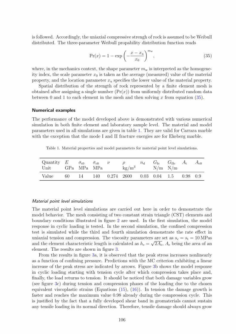
The performance of the model developed above is demonstrated with various numericalsimulation in both finite element and laboratory sample level. The material and modelparameters used in all simulations are given in table 1. They are valid for Carrara marblewith the exception that the mode I and II fracture energies are for Ekeberg marble.

Table 1. Material properties and model parameters for material point level simulations.

Quantity E σt0 σc0 ν ρ nd GIc GIIc At Ac0

Unit GPa MPa MPa kg/m3 N/m N/m

Value 60 14 140 0.274 2600 0.03 0.04 1.5 0.98 0.9

Material point level simulations

The material point level simulations are carried out here in order to demonstrate themodel behavior. The mesh consisting of two constant strain triangle (CST) elements andboundary conditions illustrated in figure 2 are used. In the first simulation, the modelresponse in cyclic loading is tested. In the second simulation, the confined compressiontest is simulated while the third and fourth simulation demonstrate the rate effect inuniaxial tension and compression. The viscosity parameters are set as sc = st = 10 MPasand the element characteristic length is calculated as he =

√2Ae, Ae being the area of an

element. The results are shown in figure 3.From the results in figure 3a, it is observed that the peak stress increases nonlinearly

as a function of confining pressure. Predictions with the MC criterion exhibiting a linearincrease of the peak stress are indicated by arrows. Figure 3b shows the model responsein cyclic loading starting with tension cycle after which compression takes place and,finally, the load returns to tension. It should be noticed that both damage variables grow(see figure 3c) during tension and compression phases of the loading due to the chosenequivalent viscoplastic strains (Equations (15), (16)). In tension the damage growth isfaster and reaches the maximum value 0.98 already during the compression cycle. Thisis justified by the fact that a fully developed shear band in geomaterials cannot sustainany tensile loading in its normal direction. Therefore, tensile damage should always grow

106

Figure 2. Computational model for material point level simulations.

Figure 3. Simulation results for material point level simulations: confined compression test (a), cyclicloading response (b), damage evolution in cyclic loading (c), influence of loading rate in compression (d),and in tension (e).

in conjunction with the compressive (shear) damage. The reciprocal process, i.e. thecompressive damage development in tensile loading, seems unphysical. However, thisprocess is much slower as can be observed in figure 3c.

As for the strain rate effects, the model does not perform very well neither in compres-sion nor in tension. In compression, higher loading rates than those in figure 3d resultedin a non-stable response. This is, at least partly, due to the inconvenient feature of theHB criterion that the compressive strength appears squared in it. In tension, the modelresponse is typical for viscoplastic models, see figure 3e, but extremely high strain rateswere required to produce the strain rate hardening effects. While this is partly due torelatively low values of viscosity moduli used here, the more important reason seems to bethe unfavorable appearance (in denominator) of the rate-dependent tensile strength in theHoek-Brown criterion (10). The classical criteria such as Rankine, Drucker-Prager andMohr-Coulomb, have form f(σ, κ, κ) = f(σ) + σY (κ, κ) where f(σ) is some expressionof stress. As the yield stress, σY , usually depends linearly on κ, κ, these models performmuch better, see e.g. [14].

107

Laboratory sample level: confined compression and uniaxial tension tests on rock

The confined compression and uniaxial tension tests on rock are simulated in order totest the model predictions at the structural level. The mesh made of CST elements alongwith the boundary conditions are shown in figure 4a. An example of UCS distributionproduced with the Weibull approach described above when mw = 3, x0 = 140 MPa, andxu = 50 MPa is shown in figure 4b. This value 3 for Weibull shape modulus mw, calledhomogeneity index by Zhu and Tang [16], is the middle one tested by them. The othervalues they tested were 1.5 and 6 where the first makes the rock too soft as the strength(or any other material property) is too widely distributed while the second one makesthe rock more homogeneous and overly brittle- actually too brittle in the case of marblemodeled here.

As seen in figure 4b, the UCS of the numerical sample varies dramatically from ele-ment to element the lower limit being 50 MPa and the upper about 300 MPa. However,this is the case in reality as well since the rock microstructure is a complex network of mi-crodefects and grains of different minerals with highly varying material properties. Thus,the pointwise variation of UCS from a hard mineral grain, such as quartzite, in a rockto a neighboring softer mineral grain or microflaw may easily reach the magnitude of 250MPa. The UCS of a rock then, which for the present case is 140 MPa, is a macroscopiclaboratory level property emerging from the microstructural properties. More detailedelaboration on this topic is, however, beyond the scope of the present paper and is left tobe investigated in future studies. In the numerical simulations, the effect of mw is thatlower values (than 3 here) make the rock response more nonlinear and ductile and lead toconsiderably lower strengths while higher values (than 3 here) make the rock more brittleand linear with increased strengths [16].

Figure 4. Computational model (dimensions 25× 50 mm for confined compression test simulation (2702CST elements in the mesh) (a), and an example of UCS distribution in the mesh (b).

The simulations are carried out in the unconfined case and at pressure levels 20 and 40MPa. A new distribution of UCS is generated for each simulation. Moreover, the uniaxialtensile strength distribution is obtained from the UCS distribution after multiplying itby m−1 = 0.1 (inverse of the HB parameter). The constant boundary velocity applied isv = −0.1m/s. The results along with some experimental failure modes are shown in figure5. The predicted failure modes at different levels of confinement exhibit typical features

108

Figure 5. Simulation results for confined compression and uniaxial tension tests: Damage patterns whenpconf = 0 MPa (a), pconf = 20 MPa (b), pconf = 40 MPa (c), corresponding stress-stress curves (d), tensiledamage pattern in uniaxial tension (e), and the stress-stress curve (f), experimental failure mode inuniaxial test (Adapted from [18]) (g), and experimental failure modes of Wombeyan marble in confinedcompression with 0, 3.5, and 35 MPa of confining pressure (Adapted from [17]) (h).

observed in the experiments, as can be seen in figure 5h. More specifically, the unconfinedfailure mode has a major slanted macrocrack spanning the specimen but there are otherminor vertical cracks deviating from the major crack. This simulated failure mode is, bychance of course, very close to the experimental one shown in figure 5g. Under confinementof 20 MPa this secondary tensile crack formation is mostly suppressed resulting in a singleshear band (see figure 5b) which is thicker than the major crack in the unconfined case.Upon still increasing confinement to 40 MPa, the manifested failure mode is the typicalconjugate crack system (compare figure 5c to 5h) attested many times in the experimentswith marble rocks. As for the corresponding stress-strain responses, the new featuresappeared at the structural level are pre-peak nonlinearity and rounded peak part of theresponse. These are due to the statistical UCS distributions as the weak rock elementsstart to fail beyond stress level 50 MPa (the value of Weibull location parameter). Thisis a numerical representation of microcracking in the experiments. Therefore, using the

109

statistical distribution of UCS, or some other method, is necessary for realistic modelingof rock failure phenomena in confined compression. The transverse splitting failure modein uniaxial tension (simulation carried out with v = 0.01 m/s) is also correctly predicted(see figure 5e). Finally, the predicted statistical tensile strength is 11.8 MPa.

Laboratory sample level: dynamic three-point bending of a notched semi-circular disc

Dynamic bending test of a Notched Semi-Circular disc (NSC) using the Split HopkinsonPressure Bar (SHPB) device is used for measuring rock dynamic fracture toughness. Theprinciple of the computational model illustrated in figure 6 is as follows. The compressivestress wave induced by impacting striker bar is simulated as an external stress pulse, σi(t).The incident and transmitted bars are modeled with two-node standard bar elements, andthe NSC disc is meshed with the CST elements. Finally, the contacts between the bars andthe half disc are modeled by imposing kinematic contact constraints between the bar endnodes and the half disc nodes at the support support pins (P2/2). These constraints areof form ubar,z − un,z = bn where ubar,z and un,z are the axial degrees of freedom of the barnode and a rock contact node n, respectively, and bn is the distance between the bar endand rock boundary node. The contact constraints are imposed with the forward incrementLagrange multiplier method (for details see [14]). The dimensions of the half disc are 16

Figure 6. Computational model for dynamic three-point bending of notched semi-circular disc testsimulation.

mm (thickness) and 40 mm (diameter) while the depth and the width of the notch are4 mm and 1 mm, respectively. The distance between the supporting pins is 21 mm inpresent simulations. The incident and transmitted bar lengths and diameters are 1200 mmand 25 mm, respectively. In each simulation, a sine-pulse is applied as σi(t) = Ap sin(ωt)where Ap = 100 MPa, t is time, ω = 2π/T with T = 160 µs. The Weibull parameters areas above. Finally, the viscosity moduli are set to sc = st = 0.01 MPas. The simulationresults are shown in figure 7.

According to the results in figure 7, the predicted failure mode is the axial splitting ofthe disc into two halves which rotate about the contact point between the specimen andthe incident bar reported, e.g. in [19], and shown also in figure 7e on Flamboro limestone.The damage patterns attest a single macrocrack propagating from the notch and reach-ing the contact area where some secondary crack formation occurs due to high contactpressure. Moreover, some tensile damaging at the contact pin areas can be observed. Thecorresponding contact force curves are roughly similar but the curve for P1 clearly displayfailure events at the contact area realized as a sudden drop in the curve. Finally, the pre-vious simulation is repeated with higher amplitude Ap = 150 MPa. The results are shown

110

Figure 7. Simulation results for dynamic 3-point bending of NSC (pulse amplitude 100 MPa): Deformedmesh (1773 elements, magnification = 10) (a), compressive damage pattern (b), tensile damage pattern(c), the contact forces as function of real time (d), and the experimental failure modes of Flamborolimestone (Courtesy of Prof. K. Xia) (e).

Figure 8. Simulation results for dynamic 3-point bending of NSC (pulse amplitude 150 MPa): Deformedmesh (a), compressive damage pattern (b), tensile damage pattern (c), and the contact forces as functionof real time (d).

in figure 8. With the higher amplitude stress pulse, the predicted failure mode exhibitssecondary cracks initiating at the contact areas of the support pins of transmitted barand propagating to the contact area of the incident bar, see figure 8. These cracks may beobserved in the experiments but the measurements are not valid anymore since they are

111

based on the assumption that a macrocrack leading to the failure of the sample initiateat the tip of the notch. In the present simulation this is not the case as the contact forcesare not equal, i.e. there is no ”dynamic equilibrium” as can be observed in figure 8d.

Conclusions

A damage-viscoplastic model for numerical modeling of rock fracture was presented in thispaper. As the viscoplastic part was formulated with the empirical Hoek-Brown criterion,the model predicts the failure strengths of some rocks under confined compression testmore accurately than the classical linear (in confinement) criteria, such as Drucker-Prageror Mohr-Coulomb criteria. Moreover, these classical criteria usually need a tension cut-off whereas the Hoek-Brown criterion matches both the uniaxial tensile and compressivestrengths with a single surface - a computational advantage - due to its nonlinearity. How-ever, the same nonlinearity requires iterative stress integration which is a computationalloss in comparison to the linear criteria. Moreover, the present formulation of the Hoek-Brown criterion where both the compressive and tensile strengths appear explicitly asfunctions of hardening/softening variables and their rates, resulted in a model which doesnot predict strain rate effects as well as the mentioned linear models. This was observedin numerical simulations at different loading rates.

The model, nevertheless, predicts the experimental failure modes of rock under quasi-static confined compression and uniaxial tension with a reasonable accuracy. The crucialfeature in this respect is the statistical description, using the Weibull distribution, of rockstrength heterogeneity. In the simulation of dynamic three-point bending of a notchedsemi-circular disc, the model predicted the correct failure mode initiated at the notch tip.However, due to the problems in predicting strain-rate effects, some other technique toaccommodate the strain rate-effects (where they cannot be neglected) should be searched.Alternatively, the damage-plasticity model based on the Hoek-Brown criterion can beapplied to rate-independent problems.

Finally, it is noted that the strategy to extend the underlying plasticity model toaccount for damaging and rate-effects does not depend specifically on the chosen Hoek-Brown criterion but can be applied to any yield criterion. Development of the formalframework of this extension applied to general yield criterion could be a subject of furtherresearch.

Acknowledgments

Prof. Kaiwen Xia from the Impact and Fracture Laboratory of University of Toronto(Canada) is gratefully acknowledged for providing the experimental failure modes in dy-namic bending of semicircular discs made of Flamboro limestone.

References

[1] L. Jing and J.L. Hudson. Numerical methods in rock mechanics. International Jour-nal of Rock Mechanics & Mining Sciences, 39(4):409–427,2002. doi:10.1016/S1365-1609(02)00065-5

[2] W.M. Wang, L.J. Sluys, R. De Borst. Viscoplasticity for instabilities dueto strain softening and strain-rate softening. International Journal for Nu-

112

merical Methods in Engineering, 40:3839–3864,1997. doi:10.1002/(SICI)1097-0207(19971030)40:20<3839::AID-NME245>3.0.CO;2-6

[3] J. Lemaitre. A Course on Damage Mechanics, Springer-Verlag, 1990.

[4] E. Hoek, E.T. Brown. Empirical strength criterion for rock masses. Journal of theGeotechnical Engineering Division ASCE. 106(9):1013–1035,1980.

[5] P. Grassl, M. Jirasek. Damage-plastic model for concrete failure. International Journalof Solids and Structures. 43:7166–7196,2006. doi:10.1016/j.ijsolstr.2006.06.032

[6] J. Zhao. Applicability of Mohr-Coulomb and Hoek-Brown strength criteria to thedynamic strength of brittle rock. International Journal of Rock Mechanics and MiningSciences. 37:1115–1121, 2000. doi:10.1016/S1365-1609(00)00049-6

[7] L.B. Colmenares, M.D. Zoback A statistical evaluation of intact rock failure criteriaconstrained by polyaxial test data for five different rocks. International Journal of RockMechanics and Mining Sciences. 39:695–729, 2002. doi:10.1016/S1365-1609(02)00048-5

[8] E. Hoek, C. Carranza-Torres, B. Corkum. Hoek-Brown failure criterion – 2002 Edition,Proc. NARMS-TAC Conference, Toronto, 2002, 1, 267-273.

[9] J. Clausen, L. Damkilde, L. Andersen. An efficient return algorithm for nonassociatedplasticity with linear yield criteria in principal stress space. Computers and Structures85:1795–1807, 2007. doi:10.1016/j.compstruc.2007.04.002

[10] T. Saksala. Geometric return algorithm for non-associated plasticity with multipleyield planes extended to linear softening/hardening models Rakenteiden Mekaniikka(Journal of Structural Mechanics) 42:83-98, 2009.

[11] Z. Fang, J.P. Harrison. A mechanical degradation index for rock. International Jour-nal of Rock Mechanics and Mining Sciences. 38:1193–1199, 2001. doi:10.1016/S1365-1609(01)00070-3

[12] T. Saksala, A. Ibrahimbegovic. Anisotropic viscodamage-viscoplastic consistencyconstitutive model with a parabolic cap for rocks with brittle and ductile behaviour.International Journal of Rock Mechanics and Mining Sciences. 70:460–473, 2014.doi:10.1016/j.ijrmms.2014.05.019

[13] J.C. Simo, T.J.R. Hughes. Computational Inelasticity. Springer Verlag, New York,1998.

[14] T. Saksala. Damage-viscoplastic consistency model with a parabolic cap for rockswith brittle and ductile behavior under low-velocity impact loading. InternationalJournal for Numerical and Analytical Method in Geomechanics. 34:1041–1062, 2010.doi:10.1002/nag.847

[15] C.A. Tang. Numerical simulation of progressive rock failure and associated seismic-ity. International Journal of Rock Mechanics and Mining Sciences. 34:249–261, 1997.doi:10.1016/S0148-9062(96)00039-3

113

[16] W.C. Zhu, C.A. Tang. Micromechanical Model for Simulating the Fracture Processof Rock. Rock Mechanics and Rock Engineering. 37:25–56, 2004. doi:10.1007/s00603-003-0014-z

[17] M.S. Paterson. Experimental deformation and faulting in Wombeyan marble. Geo-logical Society of America Bulletin. 69:465–76.

[18] Y. Zhou, J. Zhao In: J. Zhao (Ed.), Advances in Rock Dynamics and ApplicationsChapter 1. Introduction. CRC Press, 2011.

[19] R. Chen, K. Xia, F. Dai, F. Lub, S.N. Luo. Determination of dynamic fracture param-eters using a semi-circular bend technique in split Hopkinson pressure bar testing. En-gineering Fracture Mechanics. 76:1268–1276. doi:10.1016/j.engfracmech.2009.02.001

Timo SaksalaDepartment of Mechanical Engineering and Industrial SystemsTampere University of TechnologyP.O.Box 589, FIN-33101, Tampere, Finlandtimo.saksala@tut.fi

114