D'Alembert-Lagrange!s Principal Equations, Their Origin and Applications

K. C. Park, Carlos A. Felippa

Center for Aerospace Structures

University of Colorado at Boulder

Boulder, CO 80309

Roger Ohayon

Structural Mechanics and Coupled Systems Laboratory

Conservatoire National des Arts et Metiers (CNAM)

Paris, France.

USNCCM9

San Francisco, 23-26 July 2007

Traité de Dynamique (1758) Méchanique Analytique (1788)

D’Alembert’s Principle was

reported to Académie des

Sciences in 1742.

Lagrange came to Paris from

Turin in 1787 and published

his book in 1788.

Principal Figures for Today’s Talk

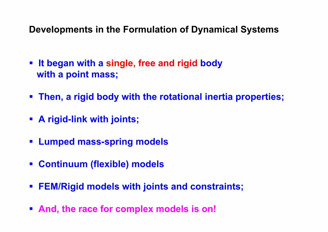
Developments in the Formulation of Dynamical Systems

! It began with a single, free and rigid body

with a point mass;

! Then, a rigid body with the rotational inertia properties;

! A rigid-link with joints;

! Lumped mass-spring models

! Continuum (flexible) models

! FEM/Rigid models with joints and constraints;

! And, the race for complex models is on!

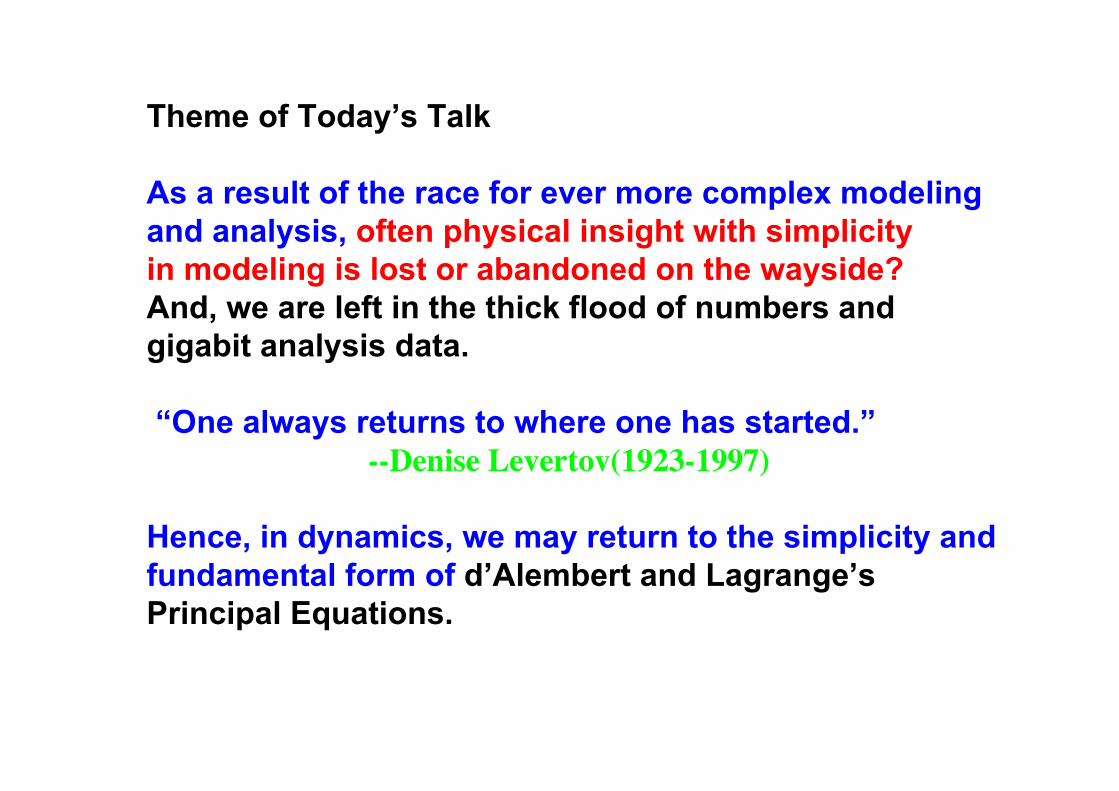
Theme of Today’s Talk

As a result of the race for ever more complex modeling

and analysis, often physical insight with simplicity

in modeling is lost or abandoned on the wayside?

And, we are left in the thick flood of numbers and

gigabit analysis data.

“One always returns to where one has started.”

--Denise Levertov(1923-1997)

Hence, in dynamics, we may return to the simplicity and

fundamental form of d’Alembert and Lagrange’s

Principal Equations.

What are D’Alembert-Lagrange Principal Equations?

Definition:

For a N-degree of freedom system,

regardless whether it is rigid or flexible,

d’Alembert-Lagrange’s principal equations

are obtained by summing all the forces and

all the moments(with respect to a point) in the system.

Symbolic Expressions:

Sum of forces (3 equations at most): ! (fi - mi ai ) = 0

Sum of moments (3 equations at most): ! {Mi + ri x (fi - mi ai )} = 0

Semantic Questions related to

the d’Alembert-Lagrange Principal Equations:

Is a floating structure in an equilibrium condition?

Or

Is a free-free substructure, partitioned from an assembled

system, in its equilibrium state?

The answer is not in the blowing wind,

but in the mathematical expressions of the d’Alembert-

Lagrange Principal Equations and their physical meaning.

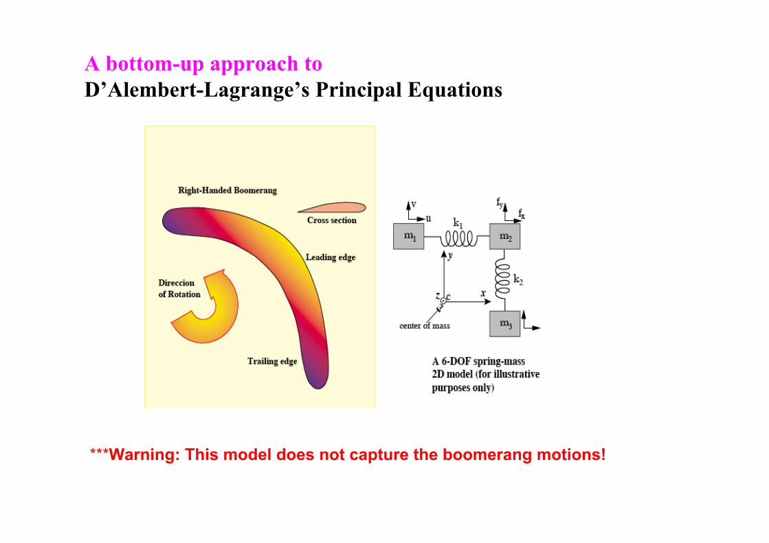
A bottom-up approach to

D’Alembert-Lagrange’s Principal Equations

***Warning: This model does not capture the boomerang motions!

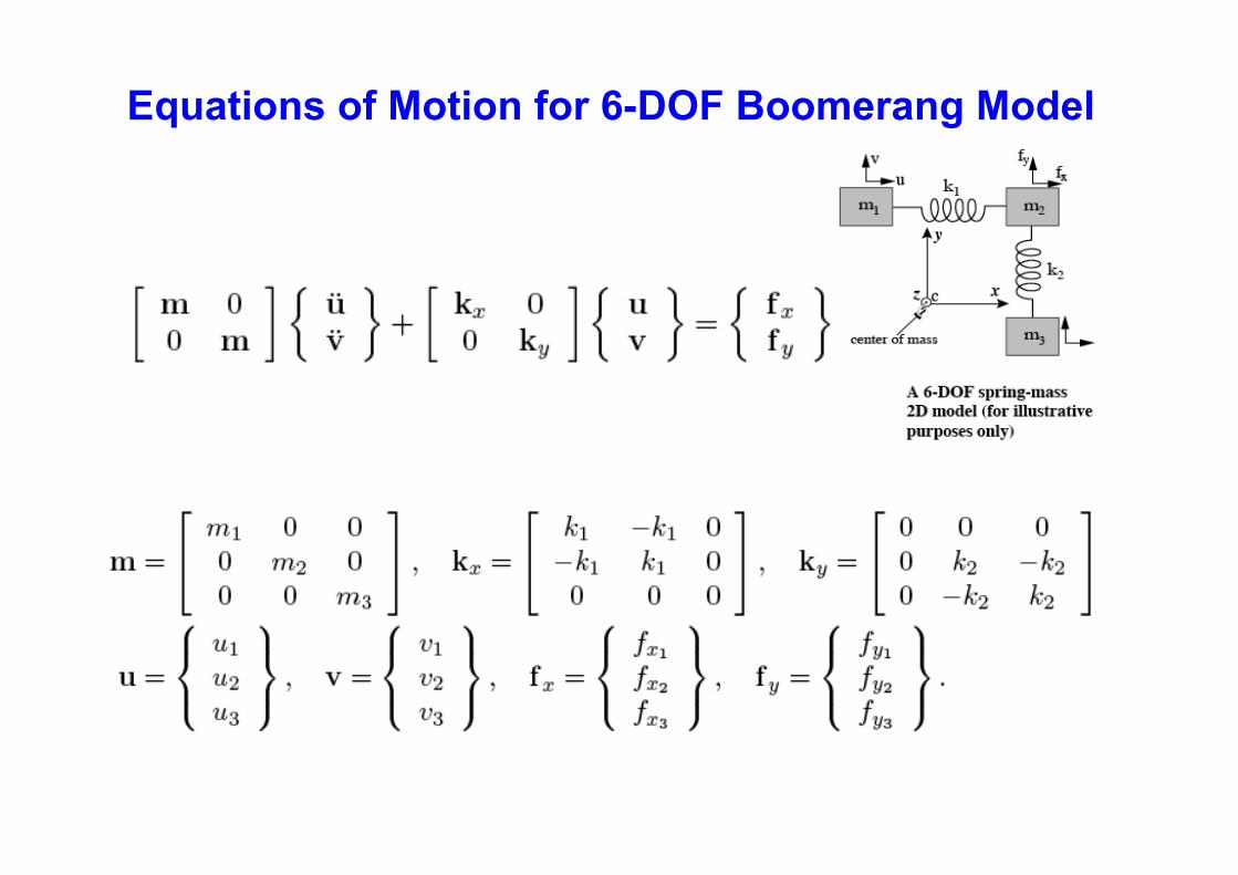
Equations of Motion for 6-DOF Boomerang Model

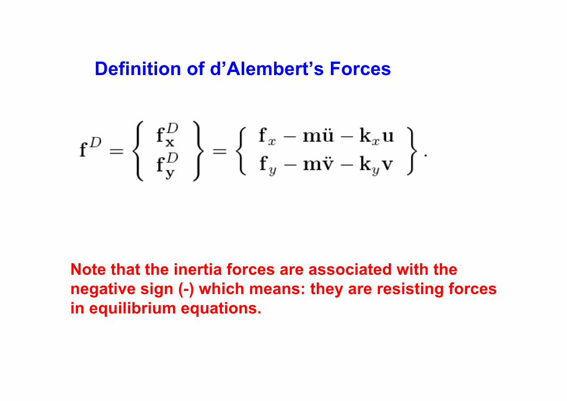
Definition of d’Alembert’s Forces

Note that the inertia forces are associated with the

negative sign (-) which means: they are resisting forces

in equilibrium equations.

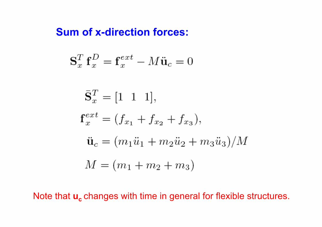
Sum of x-direction forces:

Note that uc changes with time in general for flexible structures.

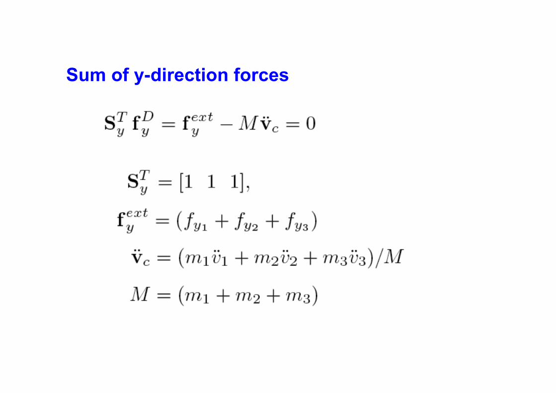
Sum of y-direction forces

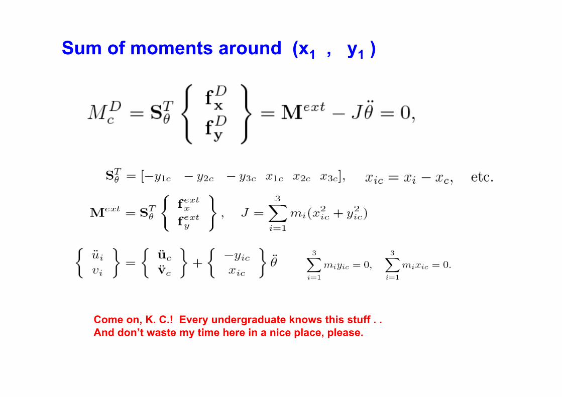
Sum of moments around (x1 , y1 )

Come on, K. C.! Every undergraduate knows this stuff . .

And don’t waste my time here in a nice place, please.

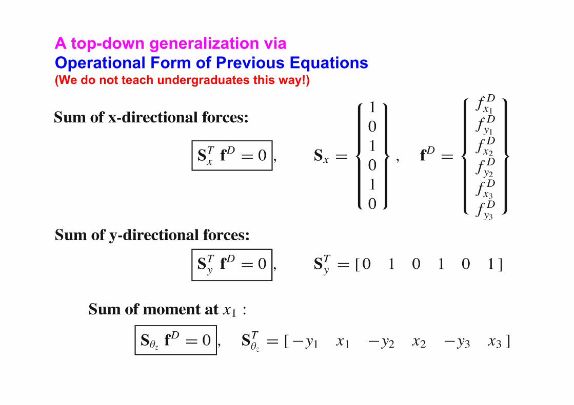
A top-down generalization via

Operational Form of Previous Equations(We do not teach undergraduates this way!)

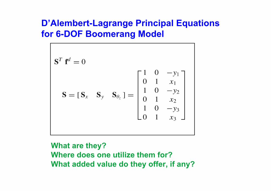
D’Alembert-Lagrange Principal Equations

for 6-DOF Boomerang Model

What are they?

Where does one utilize them for?

What added value do they offer, if any?

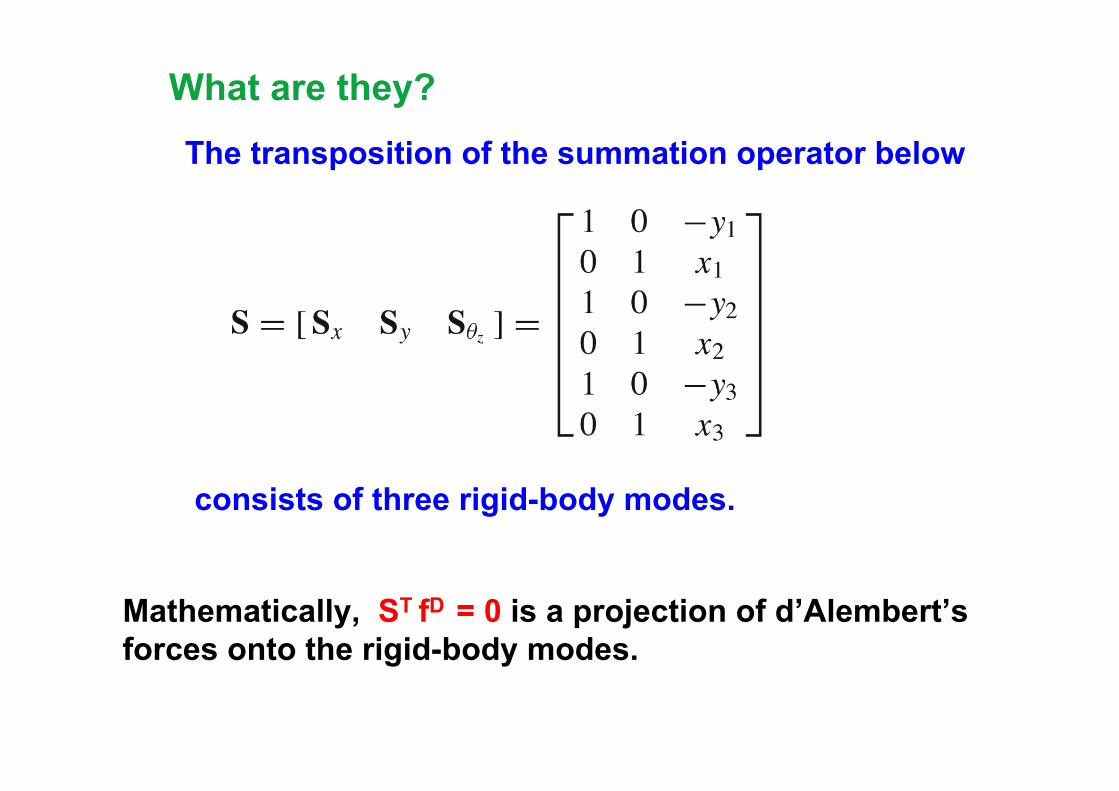
What are they?

The transposition of the summation operator below

consists of three rigid-body modes.

Mathematically, ST fD = 0 is a projection of d’Alembert’s

forces onto the rigid-body modes.

What are they? - Cont’d

The d’Alembert-Lagrange principal equations,

ST fD = 0,

represent the mean motions of flexible dynamical systems

for which the instantaneous mass center of the total system

is given, for the example problem, by

uc = (m1 u1 + m2 u2 + m3 u3 )/M, M = (m1 + m2 + m3)

so that the corresponding x-direction equation is given by

STx

fxD

= fx

- M (d2 / d t2)uc = 0

What are they? - Concluded

Physically, the three D’Alembert-Lagrange

Principal Equations given by

are self-equilibrium equations, and

ST is the self-equilibrium operator whose transposition,

S, in turn consists of the rigid-body modes, R, of the system.

R = S

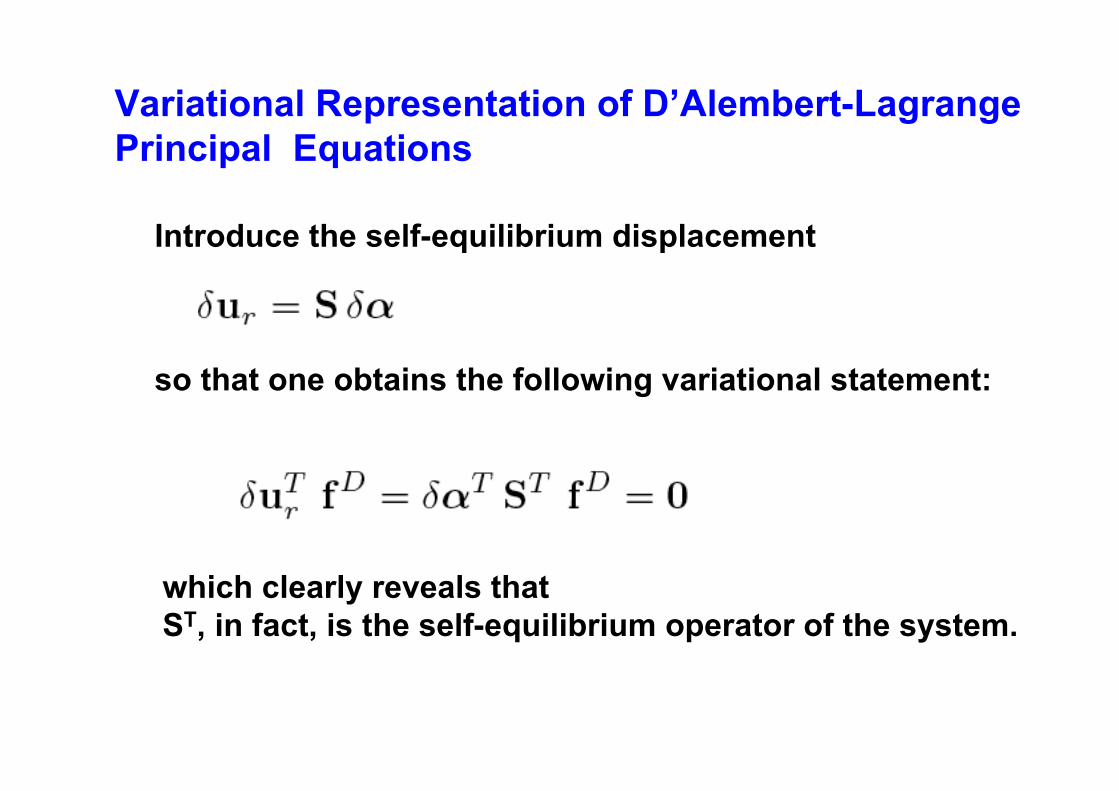
Variational Representation of D’Alembert-Lagrange

Principal Equations

Introduce the self-equilibrium displacement

which clearly reveals that

ST, in fact, is the self-equilibrium operator of the system.

so that one obtains the following variational statement:

What are they in partitioned mechanical systems?

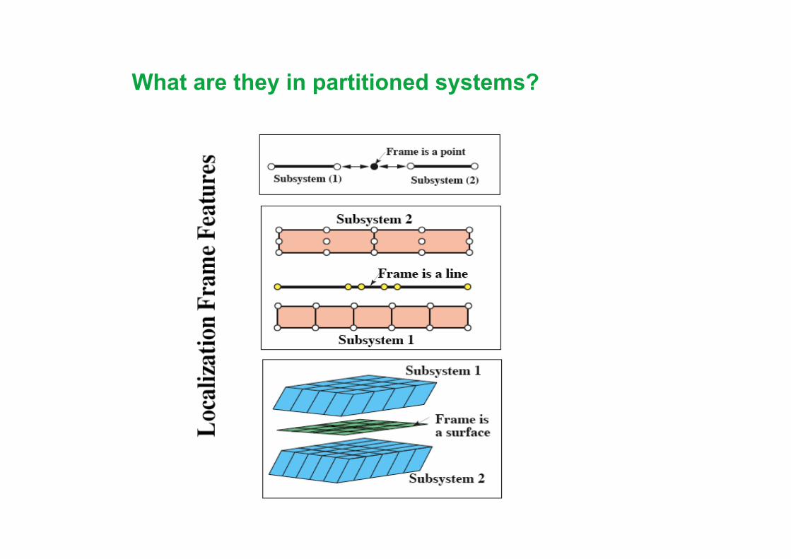
What are they in partitioned systems?

For the partitioned modeling of flexible mechanical systems,

ST fD = 0 provides self-equilibrium condition for each partition.

What are they in partitioned systems? - Concluded.

Examples for which self-equilibrium conditions are important:

Where does one utilize them for?

1. If the applied forces are known, they provide the mean

motions of the system.

2. If part or all of the forcing functions are unknown and the

mean motions are measured, they provide a least-squares

solution of the applied forces and moments. For the

example problem, they can provide a least-squares estimate

of aerodynamic forces acting on the boomerang.

3. From the theoretical point of view, the d’Alembert-

Lagrange principal equations provide the solvability

conditions for completely free or partially constrained

flexible systems, either quasi-static or dynamic. We will

examine this aspect later in the talk.

What added value do they offer, if any?

1. In the modeling of multi-physics problems, they provide

the principal (rigid-body modes) interface forces and moments,

viz., average interface forces and moments.

2. In multi-body dynamics, if properly formulated and

implemented, they provide the fundamental rigid-body motions

and the corresponding joint forces that can aid first-hand

physical insight for subsequent optimization, control and

baseline solutions for detailed analysis.

3. They facilitate the divide-and-conquer paradigm for the

modeling and solution of complex systems: a key property for

partitioned modeling and analysis.

4. In the iterative solution of large-scale problems, they provide a

crucial starting vector and subsequent filtering of residuals for

faster iterative convergence.

D’Alembert-Lagrange Principal Equations for General 3-D

Systems (Let’s get serious on their usage)

Step 1: Variational Statement of the d’Alambert-Lagrange Principal Equations:

The preceding variational observation allows us to decompose the displacement as

Step 2: The summation operator for 3-dimensional problem:

For each discrete nodal point we have

Let’s get serious on their usage - cont’d

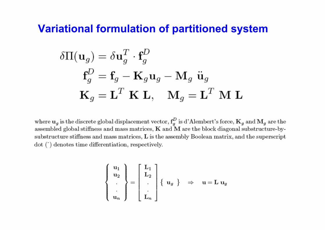
Variational formulation of partitioned system

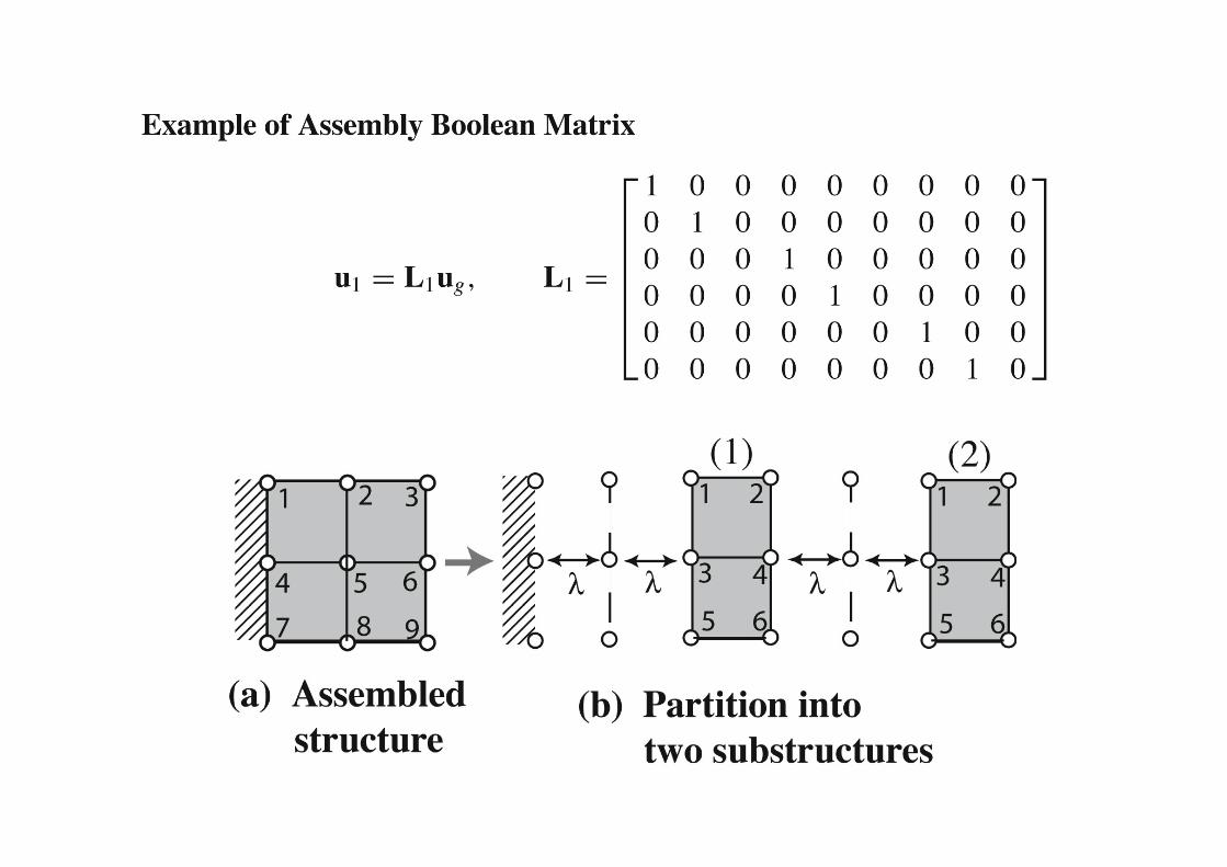
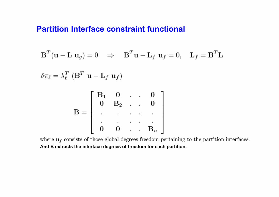
And B extracts the interface degrees of freedom for each partition.

Partition Interface constraint functional

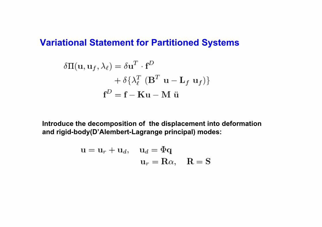
Variational Statement for Partitioned Systems

Introduce the decomposition of the displacement into deformation

and rigid-body(D’Alembert-Lagrange principal) modes:

Four-Variable Variational Formulation

for Partitioned Systems

D’Alembert-Lagrange Principal Equations for

Partitioned Systems

This equation provides the mean gross motions of the total system!

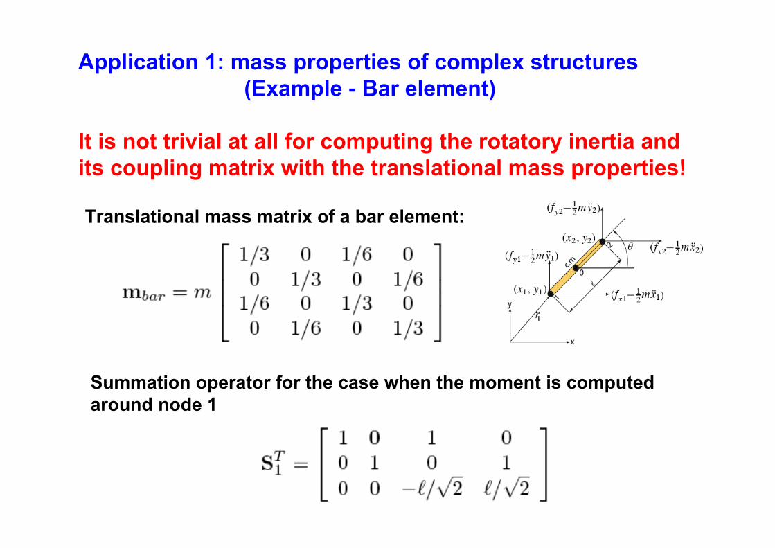
Application 1: mass properties of complex structures

(Example - Bar element)

It is not trivial at all for computing the rotatory inertia and

its coupling matrix with the translational mass properties!

Translational mass matrix of a bar element:

Summation operator for the case when the moment is computed

around node 1

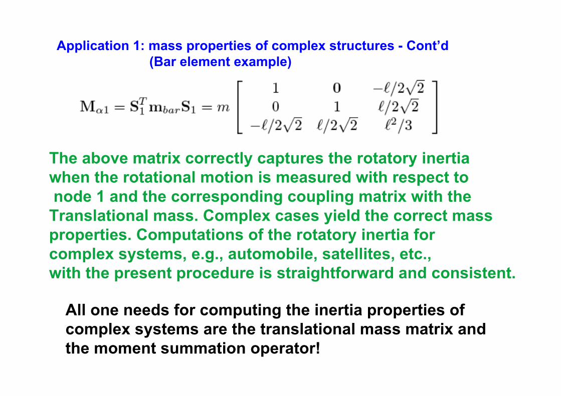
Application 1: mass properties of complex structures - Cont’d

(Bar element example)

The above matrix correctly captures the rotatory inertia

when the rotational motion is measured with respect to

node 1 and the corresponding coupling matrix with the

Translational mass. Complex cases yield the correct mass

properties. Computations of the rotatory inertia for

complex systems, e.g., automobile, satellites, etc.,

with the present procedure is straightforward and consistent.

All one needs for computing the inertia properties of

complex systems are the translational mass matrix and

the moment summation operator!

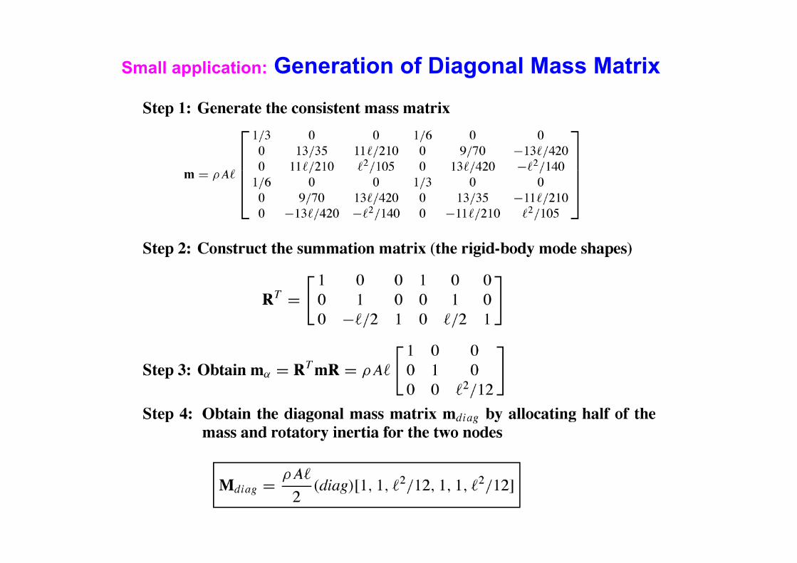
Small application: Generation of Diagonal Mass Matrix

Application 2: Solvability for unconstrained systems

under quasi-static equilibrium states

This equation is indefinite and consequently requires a delicate

care for its solution!

Partitioned equations of motion for structures:

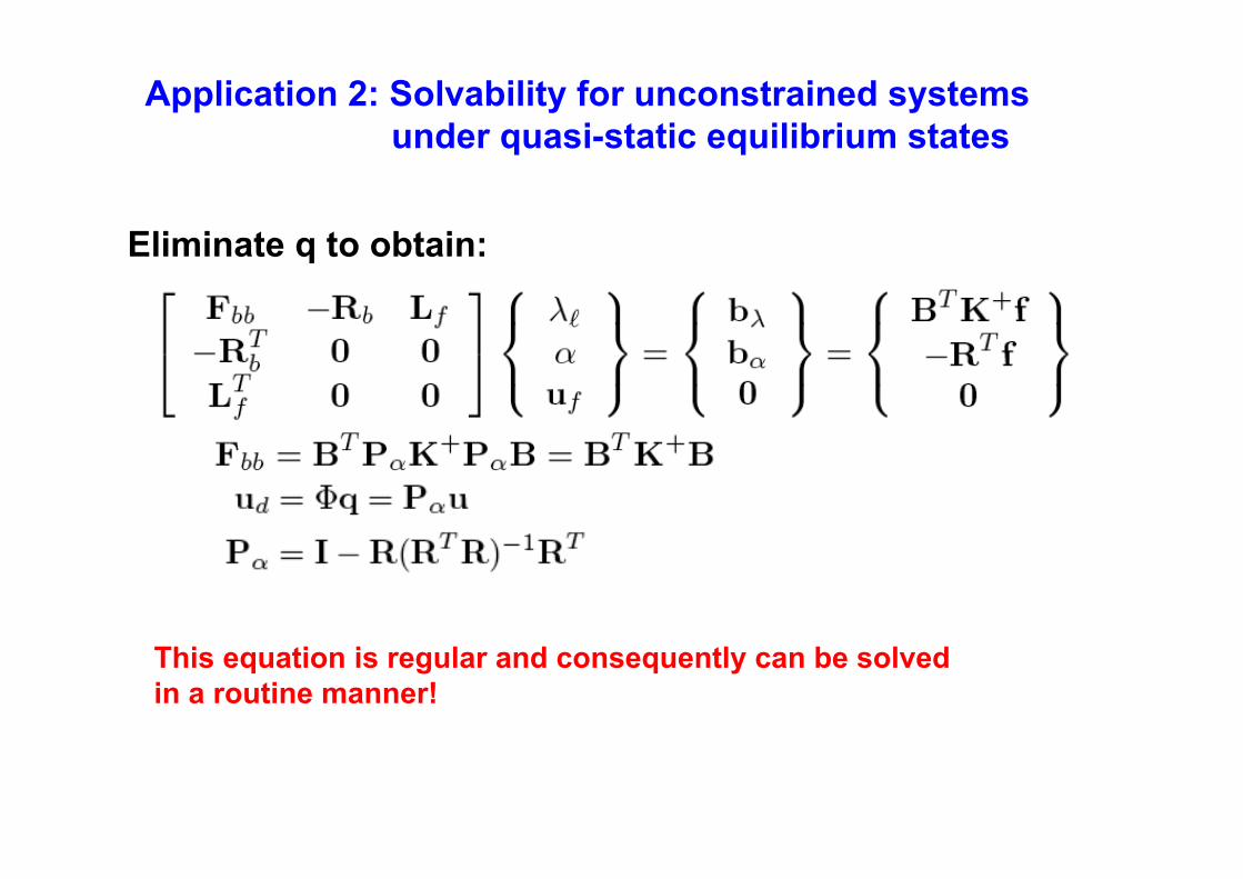
Application 2: Solvability for unconstrained systems

under quasi-static equilibrium states

Eliminate q to obtain:

This equation is regular and consequently can be solved

in a routine manner!

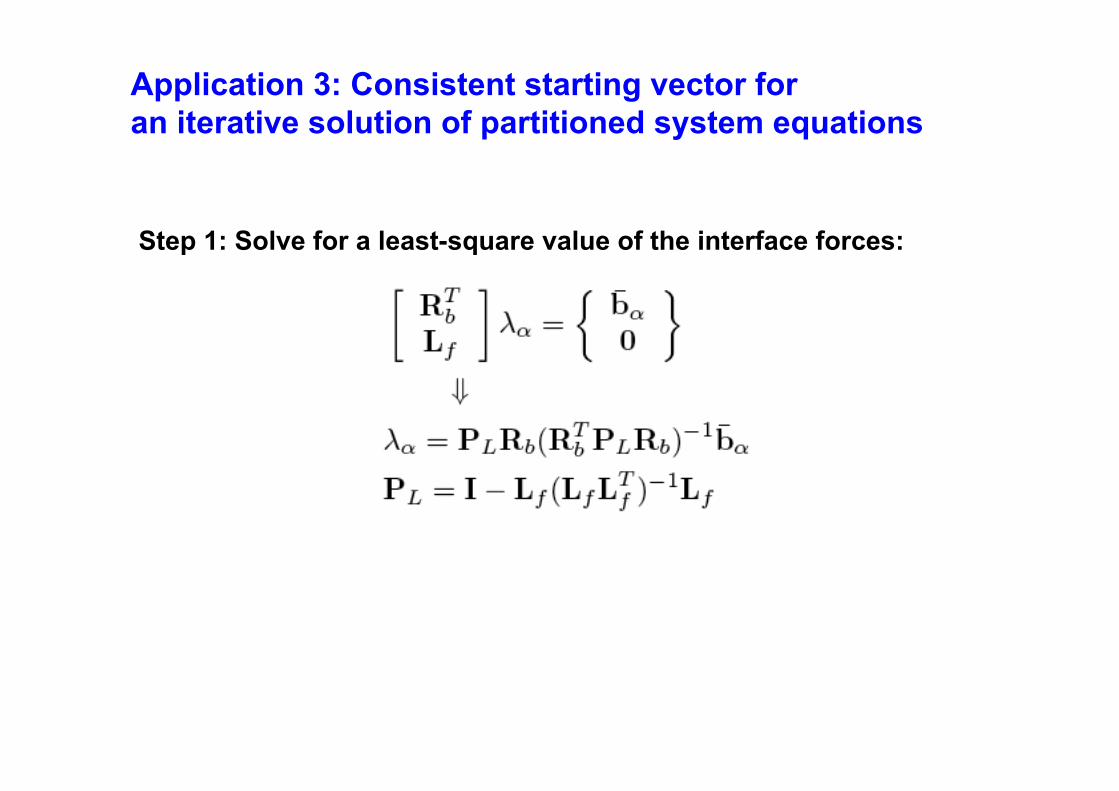
Application 3: Consistent starting vector for

an iterative solution of partitioned system equations

Step 1: Solve for a least-square value of the interface forces:

Application 3: Consistent starting vector for

an iterative solution of partitioned system equations

Step 2: Project the new iterate to be orthogonal to the interface

rigid-body modes:

in order to minimize the residual:

Future Potential Applications

A. Least-squares nominal interface forces that may

provide a preliminary design modification or control

strategy for systems with constraints.

B. Augmented solution of (q, ") for dual control

strategy development, i.e., for principal motions

and deformational motions in tandem.

C. Filtering of mean motion signals from output signals.

D. Advanced multi-physics modeling

Discussions

1. The d’Alembert-Lagrange principal equations consists of 6 rigid-body motions

regardless how large the flexible mechanical structural systems may be, and

they provide the mean motions of the overall system dynamics.

2. The rotatory inertia and its coupling terms with the translational mass

properties are obtained as part of the derivational process of the d’Alembert-

Lagrange principal equations presented herein.

3. The d’Alembert-Lagrange principal equations constitute the key solvability

condition for systems partially constrained or in completely free-free state.

4. For an iterative solution of coupled multi-physics problems, the solution of the

d’Alembert-Lagrange principal equations provides a consistent starting vector,

thus accelerating the iterative process.

5. There remains a challenge to expand the usage of the d’Alembert-Lagrane

principal equations, some of which have been outlined herein.

Viva la dynamique élémentaire!

Fin!

Question:

Can you readily get the necessary physical

insight from 108-DOF simulation results?

Wisdom from Native American Culture:

I can count five from the right fingers, and

I can count another five from the left fingers.

And, I don’t know how to count further!