D1.4 GNSS Algorithms Design
43
This project has received funding from the European Union’s Horizon 2020 research and innovation programme under Grant Agreement No 777561 Call identifier: H2020-S2RJU-2017 | Topic: S2R-OC-IP2-01-2017 – Operational conditions of the signalling and automation systems; signalling system hazard analysis and GNSS SIS characterization along with Formal Method application in railway field D1.4 – GNSS Algorithms Design Deliverable ID D1.4 Deliverable Title GNSS Algorithms Design Work Package WP1 Dissemination Level PUBLIC Version 1.15 Date 2019-01-18 Status Text Lead Editor ISMB Main Contributors ISMB, ENAC Published by the ASTRAIL Consortium Ref. Ares(2019)510811 - 29/01/2019
Transcript of D1.4 GNSS Algorithms Design

This project has received funding from the European Union’s Horizon 2020 research and innovation programme under Grant Agreement No 777561 Call identifier: H2020-S2RJU-2017 | Topic: S2R-OC-IP2-01-2017 – Operational conditions of the signalling and automation systems; signalling system
hazard analysis and GNSS SIS characterization along with Formal Method application in railway field
D1.4 – GNSS Algorithms Design
Deliverable ID D1.4
Deliverable Title GNSS Algorithms Design
Work Package WP1
Dissemination Level PUBLIC
Version 1.15
Date 2019-01-18
Status Text
Lead Editor ISMB
Main Contributors ISMB, ENAC
Published by the ASTRAIL Consortium
Ref. Ares(2019)510811 - 29/01/2019
Satellite-based Signalling and Automation Systems on Railways along with formal Method ad Moving Block Validation
Deliverable no.
Deliverable Title
Version
D1.4
GNSS Algorithms Design
1.15 – 18/01/2019
Page 2 of 43
Document History
Version Date Author(s) Description
0.0 2018-07-10 ISMB-NavSAS First draft with TOC
1.0 2018-07-12 ISMB-NavSAS NavSAS contribution inserted
1.1 2018-07-13 ISMB-NavSAS NavSAS contribution to subsection 3.1
1.2 2018-07-16 ISMB-NavSAS NavSAS contribution to subsection 3.3
1.3 2018-07-24 ISMB-MLW Draft contribution to subsection 3.2
1.4 2018-07-31 ISMB-MLW Complete draft contribution of subsection 3.2
1.5 2018-08-20 ISMB-NavSAS NavSAS contributions revised and enriched
1.6 2018-08-28 ISMB-MLW Legal Notice inserted, minor corrections
1.7 2018-08-28 ISMB-NavSAS All modifications accepted, minor corrections
1.8 2018-08-29 ISMB-MLW Modifications to subsection 3.2.1.3, based on comments received from ENAC
1.9 2018-08-31 ENAC ENAC contribution inserted
1.10 2018-08-31 ISMB-NavSAS All modifications accepted, references merged
1.11 2018-08-31 ISMB-NavSAS Minor modifications and comments introduced in section 2
1.12 2018-08-31 ENAC References resolved
1.13 2018-08-31 ISMB-NavSAS All modifications accepted, stop tracking revisions
1.14 2019-01-18 ENAC Subsection 2.3.1 has been modified to address the reviewer’s comment
1.15 2019-01-18 LINKS-NavSAS Some typo and cross-reference fixed
Legal Notice
The information in this document is subject to change without notice. The Members of the ASTRail Consortium make no warranty of any kind with regard to this document, including, but not limited to, the implied warranties of merchantability and fitness for a particular purpose. The Members of the ASTRail Consortium shall not be held liable for errors contained herein or direct, indirect, special, incidental or consequential damages in connection with the furnishing, performance, or use of this material. The Shift2Rail JU cannot be held liable for any damage caused by the Members of the ASTRail Consortium or to third parties as a consequence of implementing this Grant Agreement No 777561, including for gross negligence. The Shift2Rail JU cannot be held liable for any damage caused by any of the beneficiaries or third parties involved in this action, as a consequence of implementing this Grant Agreement No 777561. The information included in this report reflects only the authors' view and the Shift2Rail JU is not responsible for any use that may be made of such information.
Satellite-based Signalling and Automation Systems on Railways along with formal Method ad Moving Block Validation
Deliverable no.
Deliverable Title
Version
D1.4
GNSS Algorithms Design
1.15 – 18/01/2019
Page 3 of 43
Table of Contents
Document History ...................................................................................................................................................................................... 2
Legal Notice .................................................................................................................................................................................................. 2
Table of Contents ....................................................................................................................................................................................... 3
1 Introduction ........................................................................................................................................................................................ 4
1.1 Scope........................................................................................................................................................................................... 4
1.2 Organization of the document ......................................................................................................................................... 4
1.3 Related documents................................................................................................................................................................ 4
2 GNSS-centric architecture (ENAC) ............................................................................................................................................. 5
2.1 ARAIM Algorithms ................................................................................................................................................................. 7
2.2 SBAS Monitoring .................................................................................................................................................................... 8
2.3 Odometry Based Fault Diagnostic ................................................................................................................................. 10
3 Algorithms for improved positioning availability (ISMB) ............................................................................................... 20
3.1 Identification of operational scenarios (NavSAS) .................................................................................................... 20
3.2 Complementary technologies (MLW) .......................................................................................................................... 21
3.3 Possible approaches to integration (NavSAS) .......................................................................................................... 29
4 Algorithms for enhanced robustness against RFI (ISMB) ............................................................................................... 33
4.1 Identification of the target algorithm: Frequency Lock Loop (FLL) – equivalent ANF .............................. 33
4.2 Jammers selection ................................................................................................................................................................ 34
4.3 FLL – equivalent ANF: algorithm description ............................................................................................................ 34
4.4 Methodology for performance evaluation................................................................................................................. 37
5 Conclusions (ISMB-NavSAS) ...................................................................................................................................................... 39
List of figures .............................................................................................................................................................................................. 40
List of tables ................................................................................................................................................................................................ 40
References ................................................................................................................................................................................................... 40
Satellite-based Signalling and Automation Systems on Railways along with formal Method ad Moving Block Validation
Deliverable no.
Deliverable Title
Version
D1.4
GNSS Algorithms Design
1.15 – 18/01/2019
Page 4 of 43
1 Introduction
This document is the deliverable D1.4 of the ASTRail project; it includes the outcomes of Task 1.6 “GNSS Algorithm Analysis and Design” carried out by ISMB with the contribution of ENAC.
1.1 Scope
Al already mentioned in [RD.1], the introduction of the Global Navigation Satellite Systems (GNSS) technology in safety railway applications is the new challenge. A safe train positioning is, indeed, one of the technical demonstrator of the Innovation Programme 2 (IP2) – Advanced Traffic Management and Control Systems – of the EU-H2020 Shift2Rail (S2R) project [1], aiming to develop a fail-safe, multi-sensor GNSS-based train positioning system as an add-on to the current European Rail Traffic Management System/European Train Control System (ERTMS/ETCS). In [RD.1] the main impairments affecting the GNSS signal in a railway scenario, i.e. multipath and Radio-Frequency Interference (RFI), have been classified and discussed. The next step is therefore to define a GNSS-centric architecture suitable for positioning in the railway environment, i.e. robust to such impairments. Thus, the selection and design of specific algorithms for GNSS receivers able to cope with the mentioned vulnerabilities is the focus of the Task 1.6 and the content of this deliverable. In particular, to improve the positioning availability in case of reduced visibility of GNSS satellites, the integration with other sources of positioning information will be examined and discussed, while to enhance the RFI resilience, a specific algorithm for the detection and mitigation of RFI signals will be selected and analysed.
1.2 Organization of the document
After the Introduction, this document can be divided in three main parts
Section 2 defines a GNSS-centric architecture suitable for positioning in the railway environment
Section 3 describes the identification of both operational scenarios and appropriate complementary technologies for enhancing GNSS positioning availability in the railway environment. Possible approaches of data fusion are also discussed
Section 4 illustrates the selection and design of a specific algorithm for the detection and mitigation of GNSS RFI
Finally, Section 5 draws some conclusions.
1.3 Related documents
ID Title Reference Version Date
[RD.1] D1.2 – Local GNSS Effects ASTRAIL_D1.2 V1.0 28/02/2018
[RD.2] D3.2 - Automatic Train Operations: implementation,
operation characteristics and technologies for the Railway field
ASTRAIL_D3.2 V1.0 28/02/2018
[RD.3] D1.5 – GNSS Solutions Report ASTRAIL_D1.5 -- 28/02/2019
[RD.4] D3.1 –State of the Art of Automated Driving technologies ASTRAIL_D3.1 V1.1 01/06/2018
Satellite-based Signalling and Automation Systems on Railways along with formal Method ad Moving Block Validation
Deliverable no.
Deliverable Title
Version
D1.4
GNSS Algorithms Design
1.15 – 18/01/2019
Page 5 of 43
2 GNSS-centric architecture (ENAC)
The Virtual Balise (VB) concept has already been studied in several projects, within which the most prominent ones are Next Generation Train Control (NGTC) and Railway High Integrity Navigation Overlay System (RHINOS) projects. NGTC WP7 Satellite Positioning provides a description of the scenario as well as the roadmap with identified key elements that need to be considered to achieve a successful adoption of satellite positioning, as part of the ERTMS and defines an extensive and stable set of safety concepts around the VB concept. Below an extract from NGTC Deliverable D7.1 ([2]) explaining VB application is provided. The VB application is based on using GNSS for the only and sole purpose of providing an absolute positioning reference at discrete locations along the track, allowing a reduction of Eurobalises installation. However, Eurobalises are still foreseen in those emplacements where the signal-in-space (SIS) does not meet the GNSS performance requirements. To enable the VB functionality, the ETCS on-board unit shall include a new component, named as Virtual Balise Reader (VBR) which processes GNSS signals and provides balise messages, emulating the BTM, so the ETCS on-board does not actually distinguish if the balise message received comes from a virtual or a physical one. The VBR will employ a GNSS receiver with a PVT (position, velocity and time) unit and a database.
A GNSS receiver for processing the SIS from the augmentation system and GNSS satellites.
The PVT unit provides a PVT solution for computing the train confidence interval (protection level).
A VBR database for storing VB locations in the vicinity, providing a balise message to the ETCS on-board unit when a match between the received GNSS and stored position occurs.
For the VB functionality, there is no need to provide and guarantee GNSS services in a large region continuously since the performance requirements are only required at certain locations where the VB is placed. So GNSS services only need to be available at certain locations, considering that continuity as a concept is provided by the odometry subsystem. Within RHINOS project, performance analytical models and a Strengths, Weaknesses Opportunities, Threats SWOT analysis have been applied to select the candidate Augmentation and Integrity Monitoring (AIM) subsystem architectures for RHINOS reference architecture. As well, the analytical model of the GNSS based Virtual Balise Reader performances assessment has been reviewed. Moreover, algorithms for multiple track discrimination have been investigated, and a qualitative comparative analysis between the proposed On Board Unit (OBU) Integrity Monitoring Methods has been performed. Finally, as result of the previous analysis, Advanced Receiver Autonomous Integrity Monitoring (ARAIM) has been selected as the OBU Reference Architecture. Below a scheme is provided which is a modification of an abstraction of the RHINOS project concept that reflects VB based on-board architecture augmented as necessary by ARAIM [3], and other Differential GNSS (DGNSS) based augmentations [4][5].
Satellite-based Signalling and Automation Systems on Railways along with formal Method ad Moving Block Validation
Deliverable no.
Deliverable Title
Version
D1.4
GNSS Algorithms Design
1.15 – 18/01/2019
Page 6 of 43
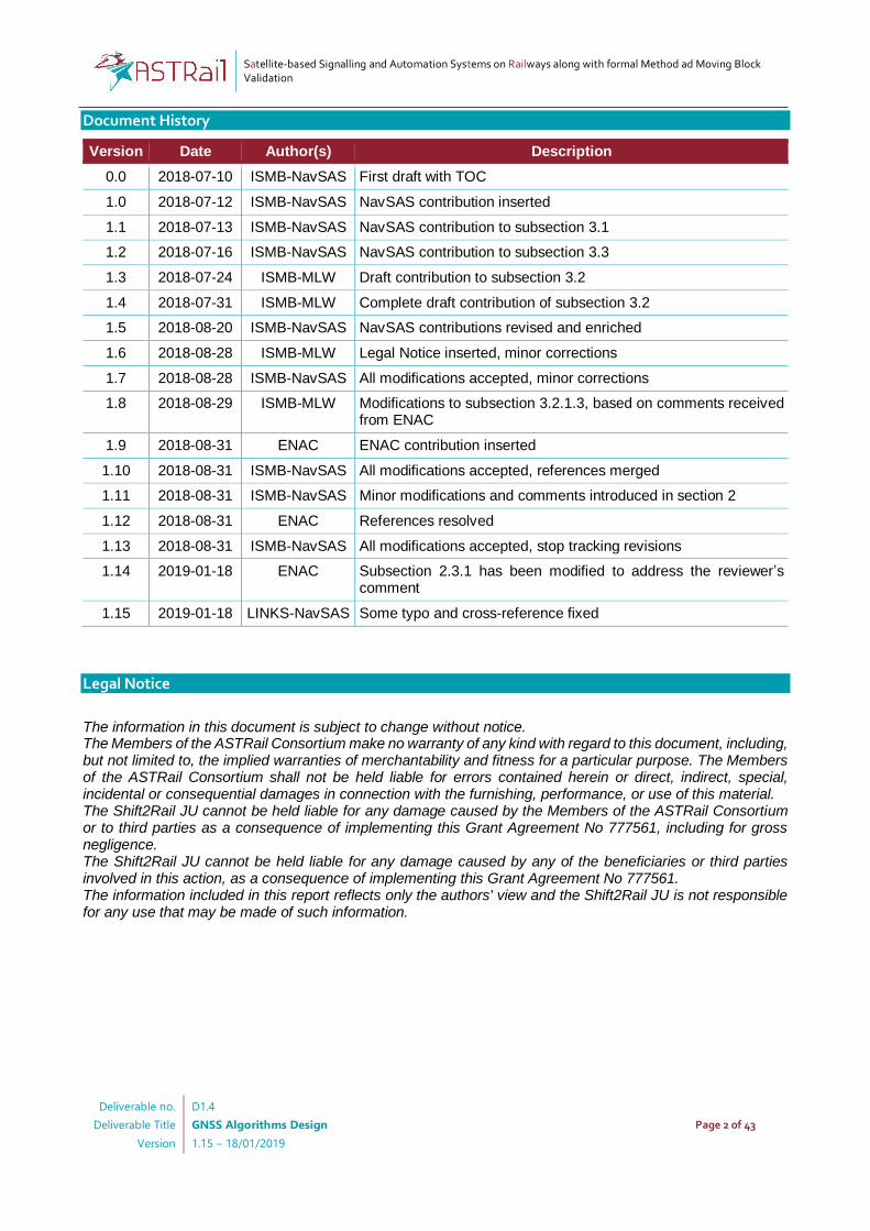
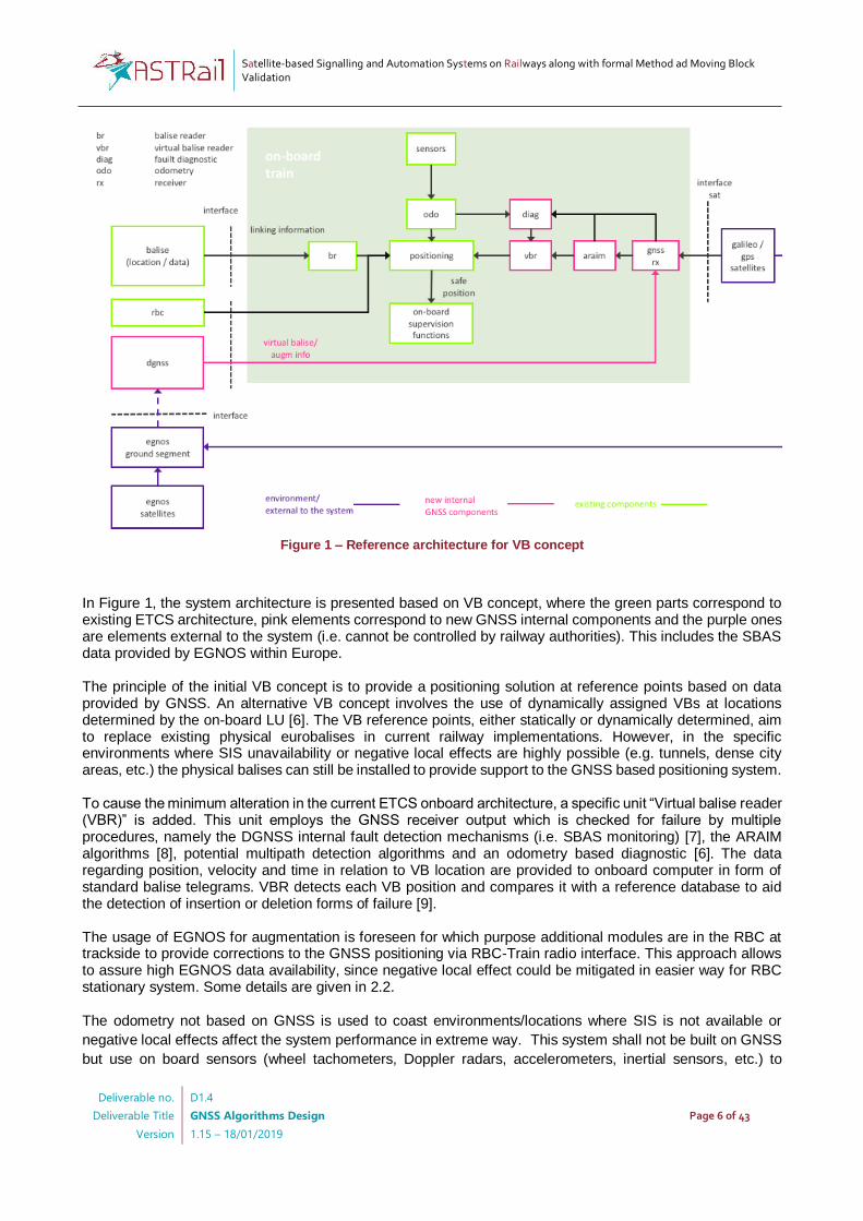
Figure 1 – Reference architecture for VB concept
In Figure 1, the system architecture is presented based on VB concept, where the green parts correspond to existing ETCS architecture, pink elements correspond to new GNSS internal components and the purple ones are elements external to the system (i.e. cannot be controlled by railway authorities). This includes the SBAS data provided by EGNOS within Europe. The principle of the initial VB concept is to provide a positioning solution at reference points based on data provided by GNSS. An alternative VB concept involves the use of dynamically assigned VBs at locations determined by the on-board LU [6]. The VB reference points, either statically or dynamically determined, aim to replace existing physical eurobalises in current railway implementations. However, in the specific environments where SIS unavailability or negative local effects are highly possible (e.g. tunnels, dense city areas, etc.) the physical balises can still be installed to provide support to the GNSS based positioning system. To cause the minimum alteration in the current ETCS onboard architecture, a specific unit “Virtual balise reader (VBR)” is added. This unit employs the GNSS receiver output which is checked for failure by multiple procedures, namely the DGNSS internal fault detection mechanisms (i.e. SBAS monitoring) [7], the ARAIM algorithms [8], potential multipath detection algorithms and an odometry based diagnostic [6]. The data regarding position, velocity and time in relation to VB location are provided to onboard computer in form of standard balise telegrams. VBR detects each VB position and compares it with a reference database to aid the detection of insertion or deletion forms of failure [9]. The usage of EGNOS for augmentation is foreseen for which purpose additional modules are in the RBC at trackside to provide corrections to the GNSS positioning via RBC-Train radio interface. This approach allows to assure high EGNOS data availability, since negative local effect could be mitigated in easier way for RBC stationary system. Some details are given in 2.2. The odometry not based on GNSS is used to coast environments/locations where SIS is not available or
negative local effects affect the system performance in extreme way. This system shall not be built on GNSS
but use on board sensors (wheel tachometers, Doppler radars, accelerometers, inertial sensors, etc.) to
Satellite-based Signalling and Automation Systems on Railways along with formal Method ad Moving Block Validation
Deliverable no.
Deliverable Title
Version
D1.4
GNSS Algorithms Design
1.15 – 18/01/2019
Page 7 of 43
provide solution independency. A method for diagnosing failures using odometry is being developed and is
presented in 2.3.
2.1 ARAIM Algorithms
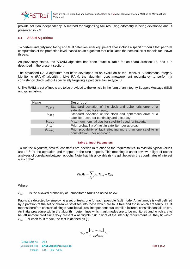
To perform integrity monitoring and fault detection, user equipment shall include a specific module that perform computation of the protection level, based on an algorithm that calculates the nominal error models for known threats. As previously stated, the ARAIM algorithm has been found suitable for on-board architecture, and it is described in the present section. The advanced RAIM algorithm has been developed as an evolution of the Receiver Autonomous Integrity Monitoring (RAIM) algorithm. Like RAIM, the algorithm uses measurement redundancy to perform a consistency check without specifically targeting a particular failure type [8]. Unlike RAIM, a set of inputs are to be provided to the vehicle in the form of an Integrity Support Message (ISM) and given below:
Name Description
𝝈𝑼𝑹𝑨,𝒊 Standard deviation of the clock and ephemeris error of a satellite 𝑖 used for integrity
𝝈𝑼𝑹𝑬,𝒊 Standard deviation of the clock and ephemeris error of a satellite 𝑖 used for continuity and accuracy
𝒃𝒏𝒐𝒎,𝒊 Maximum nominal bias for satellite 𝑖 used for integrity
𝑷𝒔𝒂𝒕,𝒊 Prior probability of fault in satellite 𝑖 per approach
𝑷𝒄𝒐𝒏𝒔𝒕,𝒊 Prior probability of fault affecting more than one satellite in constellation 𝑖 per approach
Table 1: Input Parameters
To run the algorithm, several constants are needed in relation to the requirements. In aviation typical values are 10−7 for the operation and mapped to the single epoch. This mapping is under review in light of recent analyses of correlation between epochs. Note that this allowable risk is split between the coordinates of interest 𝑞 such that:
𝑃𝐻𝑀𝐼 = ∑ 𝑃𝐻𝑀𝐼𝑞
𝑞
+ 𝑃𝑁𝑀
Where:
𝑃𝑁𝑀 is the allowed probability of unmonitored faults as noted below.
Faults are detected by employing a set of tests, one for each possible fault mode. A fault mode is well defined by a partition of the set of available satellites into those which are fault free and those which are faulty. Fault modes therefore consists of single satellite failures, independent dual satellite failures, constellation failure etc. An initial procedure within the algorithm determines which fault modes are to be monitored and which are to be left unmonitored since they present a negligible risk in light of the integrity requirement i.e. they fit within 𝑃𝑁𝑀 . For each fault mode, the test is defined as [8]:
𝜏𝑘𝑞 =|𝑥𝑘𝑞 − 𝑥0𝑞|
𝐾𝑓𝑎,𝑞𝜎𝑠𝑠,𝑘𝑞
≤ 1
Satellite-based Signalling and Automation Systems on Railways along with formal Method ad Moving Block Validation
Deliverable no.
Deliverable Title
Version
D1.4
GNSS Algorithms Design
1.15 – 18/01/2019
Page 8 of 43
Where:
𝑥0𝑞 is the 𝑞 coordinate for the full set solution
𝑥𝑘𝑞 is the 𝑞 coordinate for the subset solution 𝑘
𝐾𝑓𝑎,𝑞 is the inverse of a unit variance Gaussian distribution for probability 𝑃𝑓𝑎,𝑞
2𝑁𝑓𝑎𝑢𝑙𝑡 𝑚𝑜𝑑𝑒𝑠.
𝜎𝑠𝑠,𝑘𝑞 is the standard deviation of the solution separation (the difference 𝑥𝑘𝑞 − 𝑥0𝑞)
The fullset and subset solutions are obtained using a weighted least squares estimation:
𝑥𝑘𝑞 = (𝐺𝑇𝑊𝑘𝐺)−1𝐺𝑇𝑊𝑘𝑧
Where:
𝑧 the vector of measurements following linearisation
𝐺 is the geometry matrix following linearization of the measurement equations relating the states to the
measurements
𝑊𝑘 is the weighting matrix and 𝑊𝑘(𝑖, 𝑖) = Σ𝑖𝑛𝑡−1 (𝑖, 𝑖) if 𝑖 is fault free in 𝑘 and 𝑊𝑘(𝑖, 𝑖) = 0 otherwise
The protection level is formed as the solution of [10]:
2𝑄 (𝑙𝑞 − 𝑏0𝑞
𝜎0𝑞
) + ∑ 𝑝𝑘𝑄 (𝑙𝑞 − 𝐾𝑓𝑎,𝑞𝜎𝑠𝑠,𝑘𝑞 − 𝑏𝑘𝑞
𝜎𝑘𝑞
)
𝑁𝑓𝑎𝑢𝑙𝑡 𝑚𝑜𝑑𝑒𝑠
𝑘=1
= 𝑃𝐻𝑀𝐼𝑞
Where:
𝑄 is the right tail CDF of the Gaussian distribution.
𝑏𝑘𝑞 is the projected worst case nominal bias under fault mode 𝑘 in the direction 𝑞
𝜎𝑘𝑞 is the standard deviation of the position subset solution 𝑘 in direction 𝑞
2.2 SBAS Monitoring
The SBAS integrity concept [5] is based on splitting the operational integrity risk between the vehicle and SBAS ground segment as shown in the bottom right . The Fault Free case is handled by the vehicle’s receiver determining a protection level. The ground segment is then tasked with providing the differential corrections and ensuring that they are fault free with a probability of 10-7 per operational period being the Target Safety Level (TLS) 1e-8 per approach (with exposure time = 150 seconds). SBAS has been certified in the aviation sector for vertical operations and for lateral guidance operations only with 150s and 3600s operations respectively. The vehicle-based protection level 𝑙0 that is standardised for aviation is given as follows:

Satellite-based Signalling and Automation Systems on Railways along with formal Method ad Moving Block Validation
Deliverable no.
Deliverable Title
Version
D1.4
GNSS Algorithms Design
1.15 – 18/01/2019
Page 9 of 43
𝑙0 = 𝑘𝑓𝑓𝑥𝜎𝑥
Where: 𝜎𝑥 is the standard deviation for the coordinate(s) of interest 𝑘𝑓𝑓𝑥 is the Gaussian multiplier relating to the allocated integrity risk for the coordinate(s) of interest
In the case that the standard deviation is in one single coordinate (e.g. vertical direction for an aircraft), the positioning error standard deviation is given as:
𝜎𝑥 = ∑ 𝑆𝑥𝑖2 𝜎𝑖
2
𝑁
𝑖=1
Where: 𝜎𝑖 is the standard deviation of the differentially corrected range from satellite 𝑖 𝑆𝑥𝑖 is the projection factor from the pseudoinverse matrix relating to the direction 𝑥 and for satellite 𝑖 In order that the protection level computed at the vehicle be fault free, the ground system monitoring must ensure the range errors are bounded sufficiently. This is achieved by the use of various monitors, in both the position and range. The exact implementation of the ground system is not made public. However, the designers have made some details available. Once again, a fault-tree analysis is performed to account for the multitude of threats including.
- Safety Processor (WAAS) / Check-Set (EGNOS) hardware failure - Corrupted measurement data - GPS satellite failure - Corrupted SBAS message between computation and broadcast - Incorrect bounding of the corrections error by the broadcast integrity data [7]
These threats are mitigated through the use of redundant hardware, Cyclic Redundancy Checks (CRC) and
the UDRE and GIVE monitors. Of the 10-7 per operation ground system allocation, 4.510-8 is allocated in WAAS to the incorrect bounding fault, with such a requirement a data driven approach is unfeasible and the mitigation must be proven through analytic techniques with data for validating any assertions used. Bounding may fail for either the FLT (fast and long-term corrections) associated to the satellite ephemeris and clock
errors or for the ionospheric corrections. The allocation is split evenly for WAAS between these two, 2.510-8 for each per operation. Finally, note that the corrections may be incorrect at any point during the approach. In the case of the FLT corrections there are 25 sets of corrections during a single 150s approach (since they
repeat each 6 seconds). This leads to an allocation at each UDRE monitor iteration of 910-10 conservatively
taking no credit for any error correlation. The notion of the Safety Processor in WAAS [11], or equivalently the Checkset in EGNOS [12], is that the data
used is independent of the processing set data which computes the corrections. Similarly, the algorithms
employed are also to be different and ‘independent’.
The UDRE monitor noise is also independent from station to station. Therefore, as state in [7], one approach to ensure that the monitor is valid is to use the following test for an allocated probability of hazardously
misleading information of 910-10 given below:
2 ∏ Φ (𝐿 − 𝑇𝑖
𝜎𝑚𝑜𝑛,𝑖
)
𝑛
𝑖=1
≤ 𝑃ℎ𝑚𝑖
Where: 𝑖 is the station index up to 𝑛

Satellite-based Signalling and Automation Systems on Railways along with formal Method ad Moving Block Validation
Deliverable no.
Deliverable Title
Version
D1.4
GNSS Algorithms Design
1.15 – 18/01/2019
Page 10 of 43
𝐿 is the limit for correct bounding, namely 5.33𝜎𝑈𝐷𝑅𝐸 𝑇𝑖 is the UDRE monitor threshold for station 𝑖 𝜎𝑚𝑜𝑛,𝑖 is the monitoring noise standard deviation for station 𝑖 Φ is the right tail Gaussian CDF Later papers from WAAS designers [13] presented more efficient algorithms, however, the full and up-to-date detail of the ground monitoring is not subject to standardization and is thus not publicly known. Similar monitoring of the bounding process is of course needed for the ionospheric corrections and associated broadcast GIVE values. What can be concluded from the SBAS integrity setup is that each ranging source corrected measurement may be modelled as a Gaussian error up to 5.33𝜎𝑈𝐷𝑅𝐸 and that the probability of any exceeding this value is
less than 10−7 within 150s. It may be possible to extend this to 0.510-7 within 1 hour since the requirement for lateral guidance in this respect is more stringent but fewer details are published.
2.3 Odometry Based Fault Diagnostic
2.3.1 Requirement Context
A number of sources have developed requirements for the failure of the VBR for a GNSS based train localisation system. The following statement is maintained from [9]-[14] relating the hazard rate. As:
3.3 × 10−10 = 2 × 𝑇𝐿 × 𝜆𝐺𝑁𝑆𝑆 Where: 𝑇𝐿 is the duration of failure 𝜆𝐺𝑁𝑆𝑆 is the rate of failure This equation is based on an equivalent one for the case of physical balise deletion [15]. However, in that case the duration of failure is limited, since linking of the balises is assumed and more importantly failures at two balise groups are independent. The likelihood of two balise groups in sequence failing is then the square of
the rate 𝜆2 and may be neglected and the time between balise crossings used as the maximum fault duration. It has been suggested to employ an odometry solution to help diagnose the presence of a GNSS fault. The rationale for this is firstly that odometry is an existing sensor for the ERTMS design, so whilst the exact form of sensor or combination of sensors (wheel speed, Doppler radar, …) may vary, an odometry solution will be available. This presents a major advantage over the costs and difficulties of adding additional new technologies beyond GNSS to rail. Secondly, odometry should help to detect sudden faults, jumps or medium to fast ramps in the GNSS position solution as such effects are not expected in nominal GNSS conditions or due odometric variations (see further details below). This approach has been partially proposed in previous work [70]–[72], although the diagnostic element is incomplete. However, the ability of odometry to detect faults depends upon the fault profile. Sharp sudden changes in the GNSS position will be easily detected by an odometry based monitor, but very slow gradual faults may be difficult to detect. For this reason, a diagnostic monitor has been developed and tests in software have begun.
2.3.2 Fault Diagnosis and Models
Satellite-based Signalling and Automation Systems on Railways along with formal Method ad Moving Block Validation
Deliverable no.
Deliverable Title
Version
D1.4
GNSS Algorithms Design
1.15 – 18/01/2019
Page 11 of 43
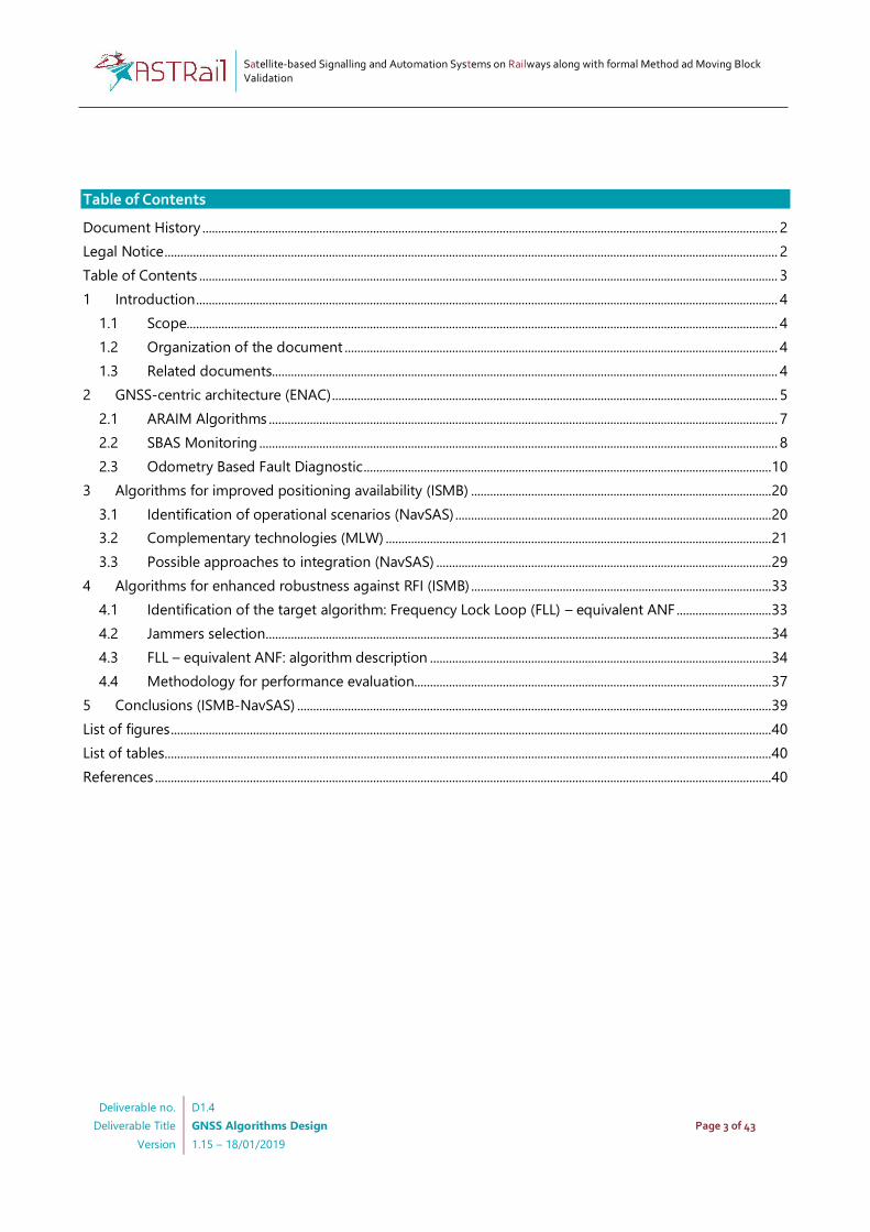
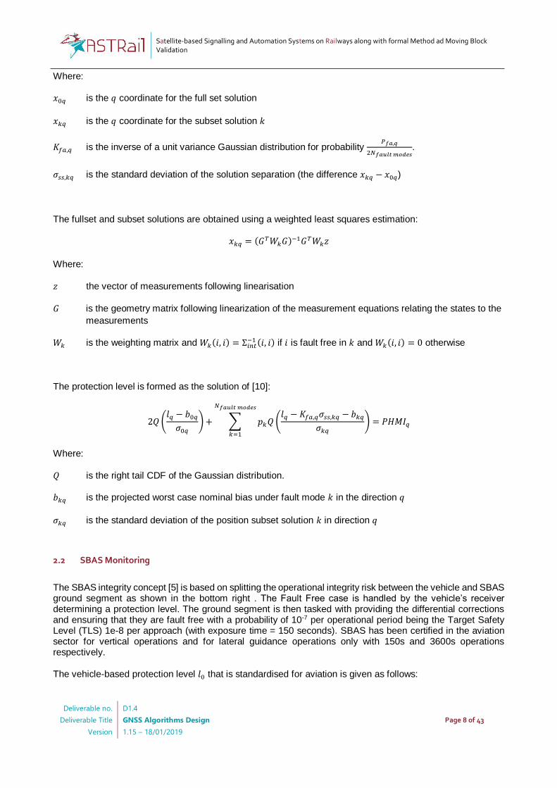
Figure 2: Odometry Diagnostic Test Software Architecture
The proposed monitor will use a bank of statistics based on the moving average, with varying
window lengths.
𝒒 = [
𝑞10
𝑞100
𝑞1000
]
𝑞𝐿 = 𝑣𝐿𝐺𝑁𝑆𝑆 − 𝑣𝐿
𝑜𝑑𝑜
𝑣𝐿𝐺𝑁𝑆𝑆(𝑡) =
1
𝐿∑ 𝑥𝐺𝑁𝑆𝑆(𝑡𝑘) − 𝑥𝐺𝑁𝑆𝑆(𝑡𝑘−1)
𝐿/𝑇
𝑘=0
Where 𝑘 is the epoch index and 𝑡𝑘 the epoch on the time axis, 𝑇 the sampling interval (i.e. time
between successive 𝑘) and 𝐿 the length of the moving average window used.
Note that in the case of constellation changes, the above relation is modified using only a common
set of satellites at the epoch of constellation change. This avoids the impact of jumps as a result of
the addition or subtraction of a satellite.
The GNSS errors are modelled as Gauss Markov processes as per GNSS standards
recommendations. The user error source refers to increased noise due to interference and to the
effects of multipath. At this stage, a simple model is used with a relatively small standard deviation.
Satellite-based Signalling and Automation Systems on Railways along with formal Method ad Moving Block Validation
Deliverable no.
Deliverable Title
Version
D1.4
GNSS Algorithms Design
1.15 – 18/01/2019
Page 12 of 43
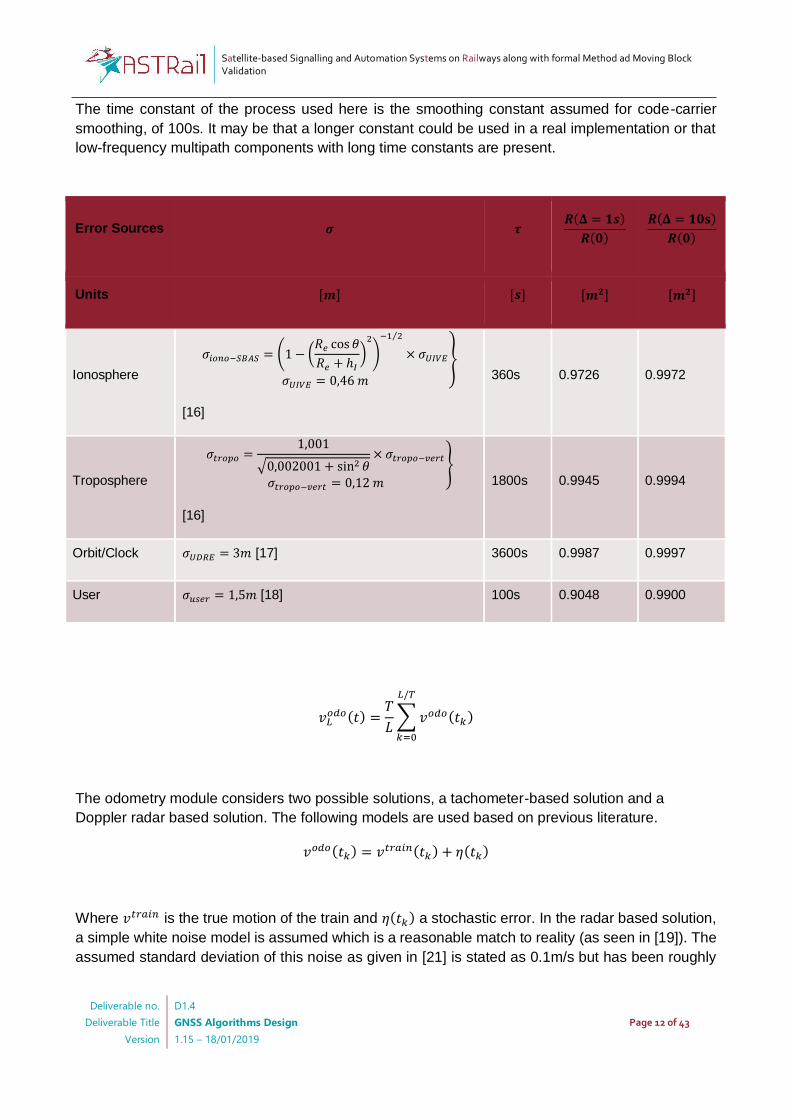
The time constant of the process used here is the smoothing constant assumed for code-carrier
smoothing, of 100s. It may be that a longer constant could be used in a real implementation or that
low-frequency multipath components with long time constants are present.
𝑣𝐿𝑜𝑑𝑜(𝑡) =
𝑇
𝐿∑ 𝑣𝑜𝑑𝑜(𝑡𝑘)
𝐿/𝑇
𝑘=0
The odometry module considers two possible solutions, a tachometer-based solution and a
Doppler radar based solution. The following models are used based on previous literature.
𝑣𝑜𝑑𝑜(𝑡𝑘) = 𝑣𝑡𝑟𝑎𝑖𝑛(𝑡𝑘) + 𝜂(𝑡𝑘)
Where 𝑣𝑡𝑟𝑎𝑖𝑛 is the true motion of the train and 𝜂(𝑡𝑘) a stochastic error. In the radar based solution,
a simple white noise model is assumed which is a reasonable match to reality (as seen in [19]). The
assumed standard deviation of this noise as given in [21] is stated as 0.1m/s but has been roughly
Error Sources 𝝈 𝝉 𝑹(𝚫 = 𝟏𝒔)
𝑹(𝟎)
𝑹(𝚫 = 𝟏𝟎𝐬)
𝑹(𝟎)
Units [𝒎] [𝒔] [𝒎𝟐] [𝒎𝟐]
Ionosphere
𝜎𝑖𝑜𝑛𝑜−𝑆𝐵𝐴𝑆 = (1 − (𝑅𝑒 cos 𝜃
𝑅𝑒 + ℎ𝐼
)2
)
−1 2⁄
× 𝜎𝑈𝐼𝑉𝐸
𝜎𝑈𝐼𝑉𝐸 = 0,46 𝑚
}
[16]
360s 0.9726 0.9972
Troposphere
𝜎𝑡𝑟𝑜𝑝𝑜 =1,001
√0,002001 + sin2 𝜃× 𝜎𝑡𝑟𝑜𝑝𝑜−𝑣𝑒𝑟𝑡
𝜎𝑡𝑟𝑜𝑝𝑜−𝑣𝑒𝑟𝑡 = 0,12 𝑚
}
[16]
1800s 0.9945 0.9994
Orbit/Clock 𝜎𝑈𝐷𝑅𝐸 = 3𝑚 [17] 3600s 0.9987 0.9997
User 𝜎𝑢𝑠𝑒𝑟 = 1,5𝑚 [18] 100s 0.9048 0.9900
Satellite-based Signalling and Automation Systems on Railways along with formal Method ad Moving Block Validation
Deliverable no.
Deliverable Title
Version
D1.4
GNSS Algorithms Design
1.15 – 18/01/2019
Page 13 of 43
estimated to be a factor of 2 lower based on the figures in [22],[23], so 0.05m/s is assumed for this
work.
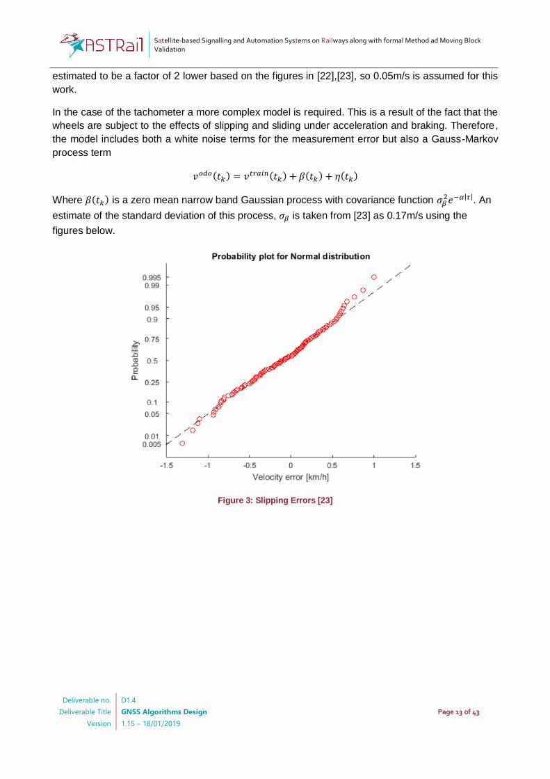
In the case of the tachometer a more complex model is required. This is a result of the fact that the
wheels are subject to the effects of slipping and sliding under acceleration and braking. Therefore,
the model includes both a white noise terms for the measurement error but also a Gauss-Markov
process term
𝑣𝑜𝑑𝑜(𝑡𝑘) = 𝑣𝑡𝑟𝑎𝑖𝑛(𝑡𝑘) + 𝛽(𝑡𝑘) + 𝜂(𝑡𝑘)
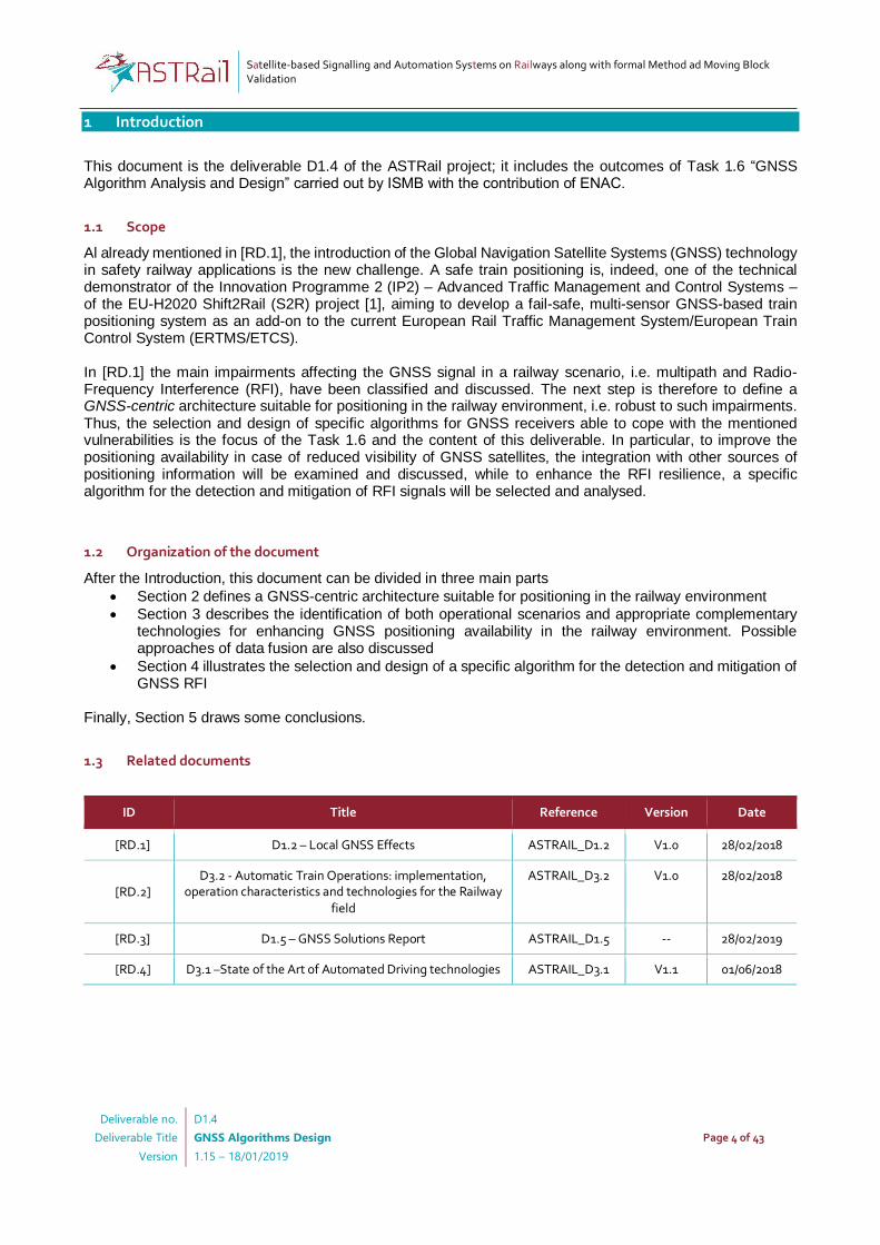
Where 𝛽(𝑡𝑘) is a zero mean narrow band Gaussian process with covariance function 𝜎𝛽2𝑒−𝛼|𝜏|. An
estimate of the standard deviation of this process, 𝜎𝛽 is taken from [23] as 0.17m/s using the
figures below.
Figure 3: Slipping Errors [23]
Satellite-based Signalling and Automation Systems on Railways along with formal Method ad Moving Block Validation
Deliverable no.
Deliverable Title
Version
D1.4
GNSS Algorithms Design
1.15 – 18/01/2019
Page 14 of 43
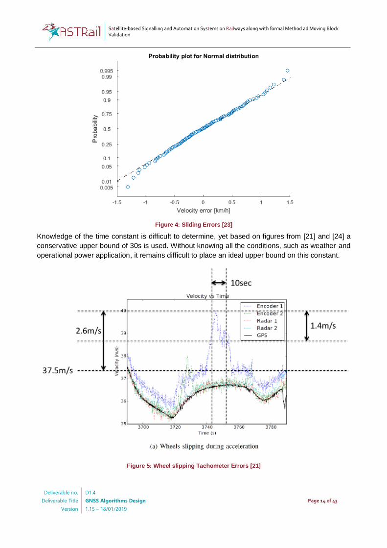
Figure 4: Sliding Errors [23]
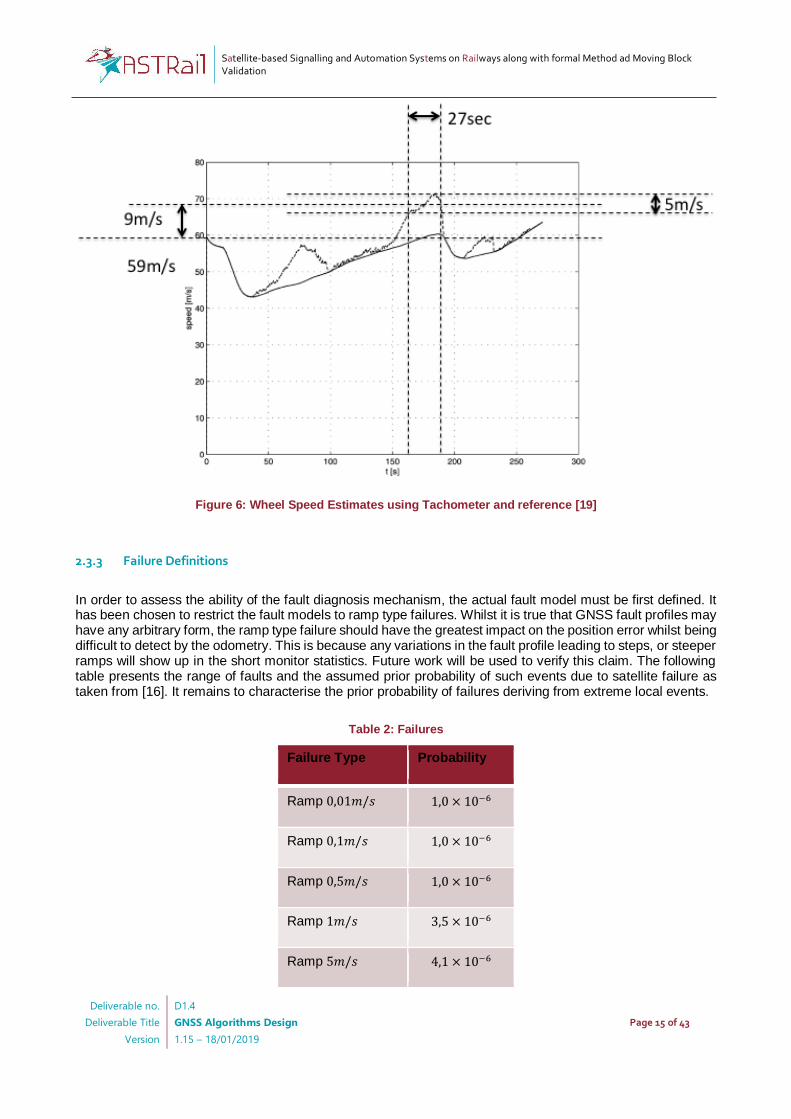
Knowledge of the time constant is difficult to determine, yet based on figures from [21] and [24] a
conservative upper bound of 30s is used. Without knowing all the conditions, such as weather and
operational power application, it remains difficult to place an ideal upper bound on this constant.
Figure 5: Wheel slipping Tachometer Errors [21]
Satellite-based Signalling and Automation Systems on Railways along with formal Method ad Moving Block Validation
Deliverable no.
Deliverable Title
Version
D1.4
GNSS Algorithms Design
1.15 – 18/01/2019
Page 15 of 43
Figure 6: Wheel Speed Estimates using Tachometer and reference [19]
2.3.3 Failure Definitions
In order to assess the ability of the fault diagnosis mechanism, the actual fault model must be first defined. It has been chosen to restrict the fault models to ramp type failures. Whilst it is true that GNSS fault profiles may have any arbitrary form, the ramp type failure should have the greatest impact on the position error whilst being difficult to detect by the odometry. This is because any variations in the fault profile leading to steps, or steeper ramps will show up in the short monitor statistics. Future work will be used to verify this claim. The following table presents the range of faults and the assumed prior probability of such events due to satellite failure as taken from [16]. It remains to characterise the prior probability of failures deriving from extreme local events.
Table 2: Failures
Failure Type Probability
Ramp 0,01𝑚/𝑠 1,0 × 10⁻⁶
Ramp 0,1𝑚/𝑠 1,0 × 10⁻⁶
Ramp 0,5𝑚/𝑠 1,0 × 10⁻⁶
Ramp 1𝑚/𝑠 3,5 × 10⁻⁶
Ramp 5𝑚/𝑠 4,1 × 10⁻⁶
Satellite-based Signalling and Automation Systems on Railways along with formal Method ad Moving Block Validation
Deliverable no.
Deliverable Title
Version
D1.4
GNSS Algorithms Design
1.15 – 18/01/2019
Page 16 of 43
In order assess with a finer resolution the array of failures, intermediate values are also tested between those given in the table above.
2.3.4 Fault Diagnosis Monitor Characterisation
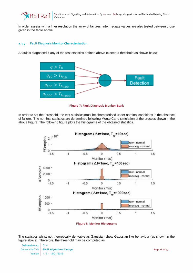
A fault is diagnosed if any of the test statistics defined above exceed a threshold as shown below.
Figure 7: Fault Diagnosis Monitor Bank
In order to set the threshold, the test statistics must be characterised under nominal conditions in the absence of failure. The nominal statistics are determined following Monte Carlo simulation of the process shown in the above Figure. The following figure plots the histograms of the obtained statistics.
Figure 8: Monitor Histograms
The statistics whilst not theoretically derivable as Gaussian show Gaussian like behaviour (as shown in the figure above). Therefore, the threshold may be computed as:
Satellite-based Signalling and Automation Systems on Railways along with formal Method ad Moving Block Validation
Deliverable no.
Deliverable Title
Version
D1.4
GNSS Algorithms Design
1.15 – 18/01/2019
Page 17 of 43
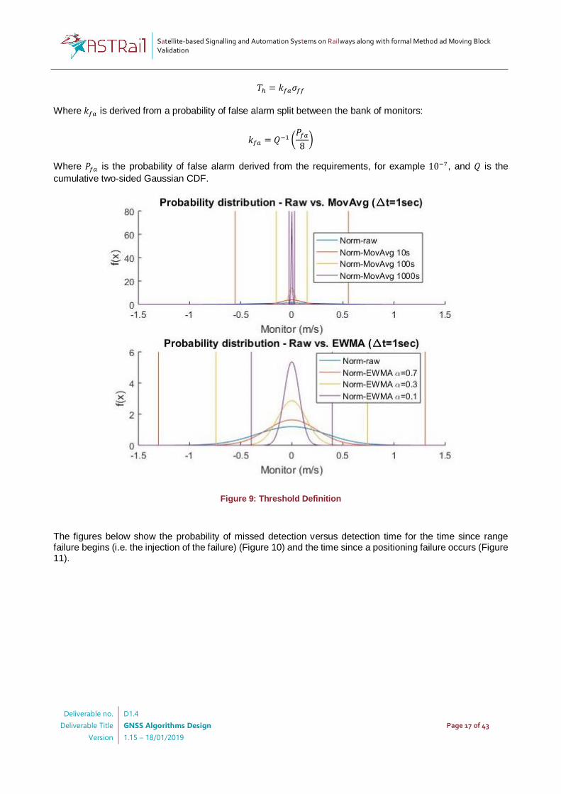
𝑇ℎ = 𝑘𝑓𝑎𝜎𝑓𝑓
Where 𝑘𝑓𝑎 is derived from a probability of false alarm split between the bank of monitors:
𝑘𝑓𝑎 = 𝑄−1 (𝑃𝑓𝑎
8)
Where 𝑃𝑓𝑎 is the probability of false alarm derived from the requirements, for example 10−7, and 𝑄 is the
cumulative two-sided Gaussian CDF.
Figure 9: Threshold Definition
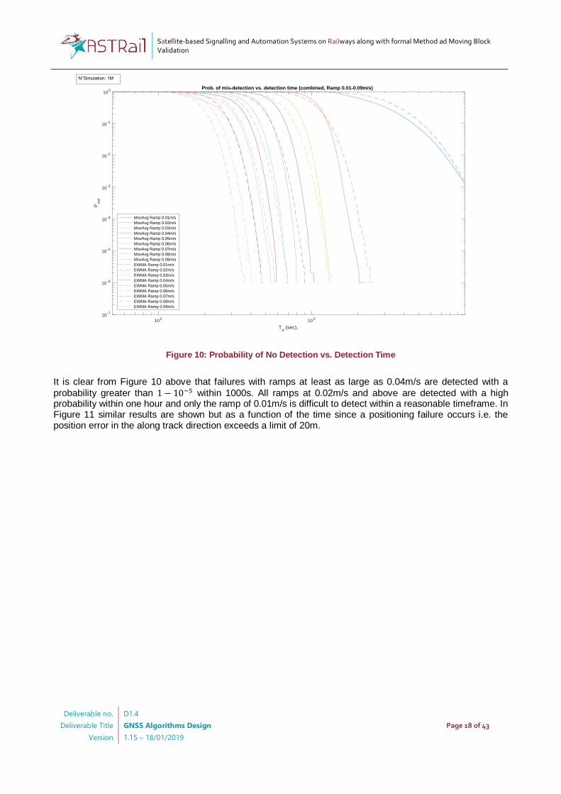
The figures below show the probability of missed detection versus detection time for the time since range failure begins (i.e. the injection of the failure) (Figure 10) and the time since a positioning failure occurs (Figure 11).
Satellite-based Signalling and Automation Systems on Railways along with formal Method ad Moving Block Validation
Deliverable no.
Deliverable Title
Version
D1.4
GNSS Algorithms Design
1.15 – 18/01/2019
Page 18 of 43
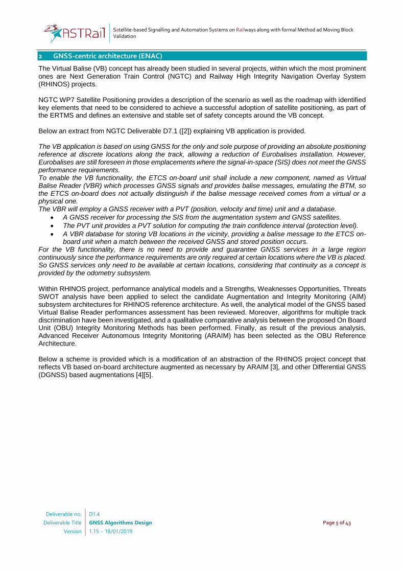
Figure 10: Probability of No Detection vs. Detection Time
It is clear from Figure 10 above that failures with ramps at least as large as 0.04m/s are detected with a
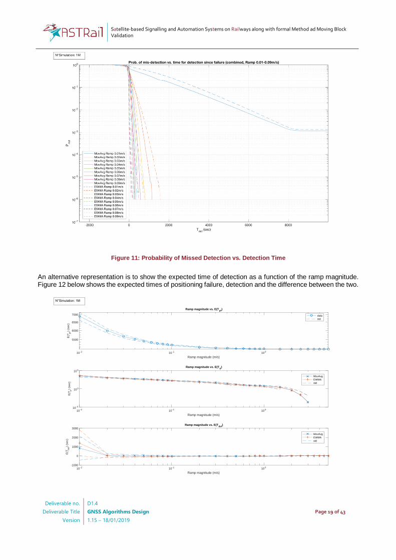
probability greater than 1 − 10−5 within 1000s. All ramps at 0.02m/s and above are detected with a high probability within one hour and only the ramp of 0.01m/s is difficult to detect within a reasonable timeframe. In Figure 11 similar results are shown but as a function of the time since a positioning failure occurs i.e. the position error in the along track direction exceeds a limit of 20m.
102
103
Td (sec),
10-7
10-6
10-5
10-4
10-3
10-2
10-1
100
Pm
d
Prob. of mis-detection vs. detection time (combined, Ramp 0.01-0.09m/s)
MovAvg Ramp 0.01m/s
MovAvg Ramp 0.02m/s
MovAvg Ramp 0.03m/s
MovAvg Ramp 0.04m/s
MovAvg Ramp 0.05m/s
MovAvg Ramp 0.06m/s
MovAvg Ramp 0.07m/s
MovAvg Ramp 0.08m/s
MovAvg Ramp 0.09m/s
EWMA Ramp 0.01m/s
EWMA Ramp 0.02m/s
EWMA Ramp 0.03m/s
EWMA Ramp 0.04m/s
EWMA Ramp 0.05m/s
EWMA Ramp 0.06m/s
EWMA Ramp 0.07m/s
EWMA Ramp 0.08m/s
EWMA Ramp 0.09m/s
N°Simulation: 1M
Satellite-based Signalling and Automation Systems on Railways along with formal Method ad Moving Block Validation
Deliverable no.
Deliverable Title
Version
D1.4
GNSS Algorithms Design
1.15 – 18/01/2019
Page 19 of 43
Figure 11: Probability of Missed Detection vs. Detection Time
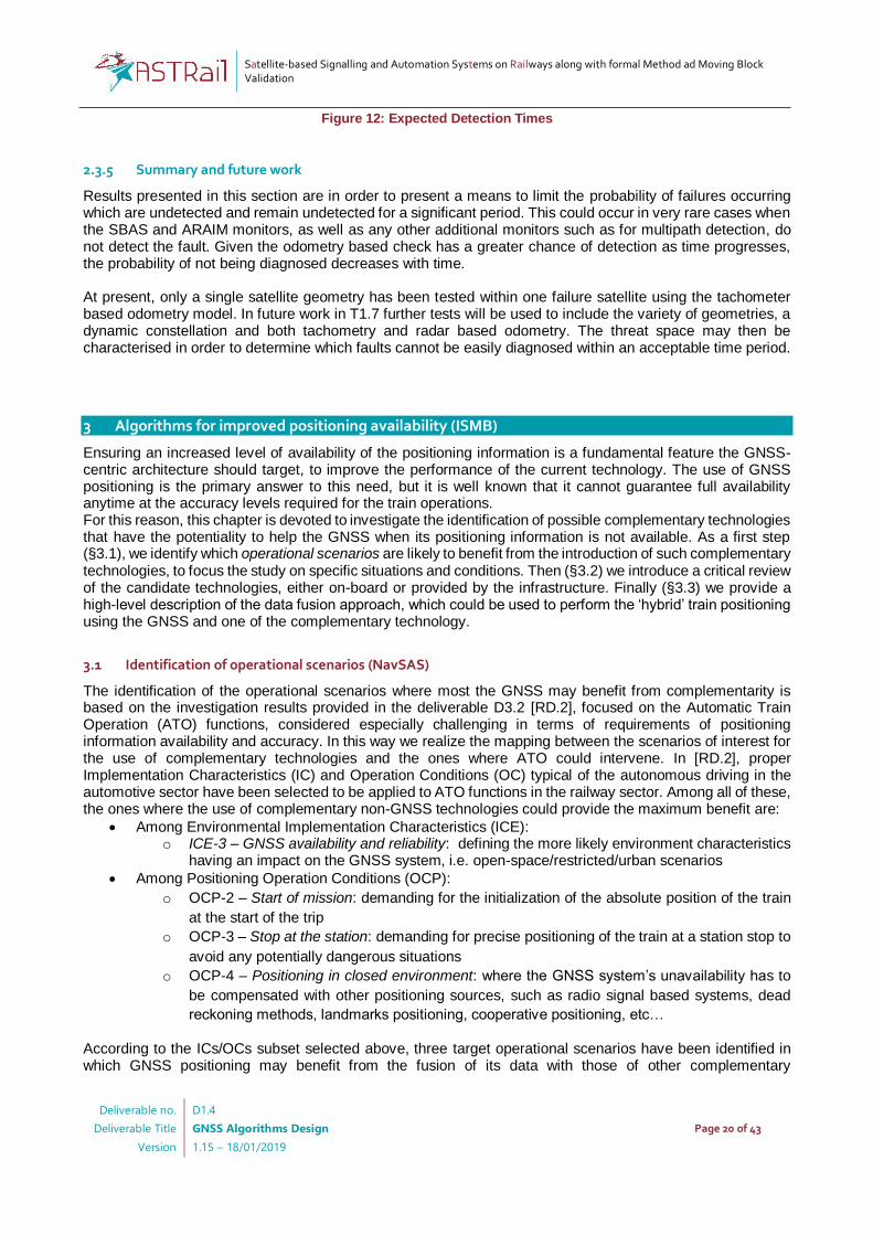
An alternative representation is to show the expected time of detection as a function of the ramp magnitude. Figure 12 below shows the expected times of positioning failure, detection and the difference between the two.
10 -2 10 -1 100
Ramp magnitude (m/s)
5500
6000
6500
7000
E(T
pf)
(se
c)
Ramp magnitude vs. E(Tpf
)
data
std
10 -2 10 -1 100
Ramp magnitude (m/s)
10 -5
100
105
E(T
d)
(sec)
Ramp magnitude vs. E(Td)
MovAvg
EWMA
std
10 -2 10 -1 100
Ramp magnitude (m/s)
-1000
0
1000
2000
3000
E(T
dsf)
(se
c)
Ramp magnitude vs. E(Tdsf
)
MovAvg
EWMA
std
N°Simulation: 1M
Satellite-based Signalling and Automation Systems on Railways along with formal Method ad Moving Block Validation
Deliverable no.
Deliverable Title
Version
D1.4
GNSS Algorithms Design
1.15 – 18/01/2019
Page 20 of 43
Figure 12: Expected Detection Times
2.3.5 Summary and future work
Results presented in this section are in order to present a means to limit the probability of failures occurring which are undetected and remain undetected for a significant period. This could occur in very rare cases when the SBAS and ARAIM monitors, as well as any other additional monitors such as for multipath detection, do not detect the fault. Given the odometry based check has a greater chance of detection as time progresses, the probability of not being diagnosed decreases with time. At present, only a single satellite geometry has been tested within one failure satellite using the tachometer based odometry model. In future work in T1.7 further tests will be used to include the variety of geometries, a dynamic constellation and both tachometry and radar based odometry. The threat space may then be characterised in order to determine which faults cannot be easily diagnosed within an acceptable time period.
3 Algorithms for improved positioning availability (ISMB)
Ensuring an increased level of availability of the positioning information is a fundamental feature the GNSS-centric architecture should target, to improve the performance of the current technology. The use of GNSS positioning is the primary answer to this need, but it is well known that it cannot guarantee full availability anytime at the accuracy levels required for the train operations. For this reason, this chapter is devoted to investigate the identification of possible complementary technologies that have the potentiality to help the GNSS when its positioning information is not available. As a first step (§3.1), we identify which operational scenarios are likely to benefit from the introduction of such complementary technologies, to focus the study on specific situations and conditions. Then (§3.2) we introduce a critical review of the candidate technologies, either on-board or provided by the infrastructure. Finally (§3.3) we provide a high-level description of the data fusion approach, which could be used to perform the ‘hybrid’ train positioning using the GNSS and one of the complementary technology.
3.1 Identification of operational scenarios (NavSAS)
The identification of the operational scenarios where most the GNSS may benefit from complementarity is based on the investigation results provided in the deliverable D3.2 [RD.2], focused on the Automatic Train Operation (ATO) functions, considered especially challenging in terms of requirements of positioning information availability and accuracy. In this way we realize the mapping between the scenarios of interest for the use of complementary technologies and the ones where ATO could intervene. In [RD.2], proper Implementation Characteristics (IC) and Operation Conditions (OC) typical of the autonomous driving in the automotive sector have been selected to be applied to ATO functions in the railway sector. Among all of these, the ones where the use of complementary non-GNSS technologies could provide the maximum benefit are:
Among Environmental Implementation Characteristics (ICE): o ICE-3 – GNSS availability and reliability: defining the more likely environment characteristics
having an impact on the GNSS system, i.e. open-space/restricted/urban scenarios
Among Positioning Operation Conditions (OCP):
o OCP-2 – Start of mission: demanding for the initialization of the absolute position of the train
at the start of the trip
o OCP-3 – Stop at the station: demanding for precise positioning of the train at a station stop to
avoid any potentially dangerous situations
o OCP-4 – Positioning in closed environment: where the GNSS system’s unavailability has to
be compensated with other positioning sources, such as radio signal based systems, dead
reckoning methods, landmarks positioning, cooperative positioning, etc…
According to the ICs/OCs subset selected above, three target operational scenarios have been identified in which GNSS positioning may benefit from the fusion of its data with those of other complementary
Satellite-based Signalling and Automation Systems on Railways along with formal Method ad Moving Block Validation
Deliverable no.
Deliverable Title
Version
D1.4
GNSS Algorithms Design
1.15 – 18/01/2019
Page 21 of 43
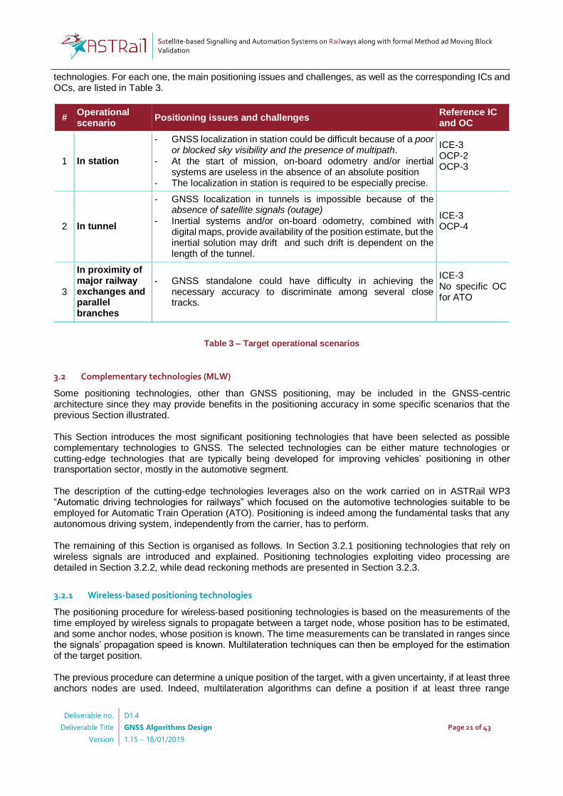
technologies. For each one, the main positioning issues and challenges, as well as the corresponding ICs and OCs, are listed in Table 3.
# Operational scenario
Positioning issues and challenges Reference IC and OC
1 In station
GNSS localization in station could be difficult because of a poor or blocked sky visibility and the presence of multipath.
At the start of mission, on-board odometry and/or inertial systems are useless in the absence of an absolute position
The localization in station is required to be especially precise.
ICE-3 OCP-2 OCP-3
2 In tunnel
GNSS localization in tunnels is impossible because of the absence of satellite signals (outage)
Inertial systems and/or on-board odometry, combined with digital maps, provide availability of the position estimate, but the inertial solution may drift and such drift is dependent on the length of the tunnel.
ICE-3 OCP-4
3
In proximity of major railway exchanges and parallel branches
GNSS standalone could have difficulty in achieving the necessary accuracy to discriminate among several close tracks.
ICE-3 No specific OC for ATO
Table 3 – Target operational scenarios
3.2 Complementary technologies (MLW)
Some positioning technologies, other than GNSS positioning, may be included in the GNSS-centric architecture since they may provide benefits in the positioning accuracy in some specific scenarios that the previous Section illustrated. This Section introduces the most significant positioning technologies that have been selected as possible complementary technologies to GNSS. The selected technologies can be either mature technologies or cutting-edge technologies that are typically being developed for improving vehicles’ positioning in other transportation sector, mostly in the automotive segment. The description of the cutting-edge technologies leverages also on the work carried on in ASTRail WP3 “Automatic driving technologies for railways” which focused on the automotive technologies suitable to be employed for Automatic Train Operation (ATO). Positioning is indeed among the fundamental tasks that any autonomous driving system, independently from the carrier, has to perform. The remaining of this Section is organised as follows. In Section 3.2.1 positioning technologies that rely on wireless signals are introduced and explained. Positioning technologies exploiting video processing are detailed in Section 3.2.2, while dead reckoning methods are presented in Section 3.2.3.
3.2.1 Wireless-based positioning technologies
The positioning procedure for wireless-based positioning technologies is based on the measurements of the time employed by wireless signals to propagate between a target node, whose position has to be estimated, and some anchor nodes, whose position is known. The time measurements can be translated in ranges since the signals’ propagation speed is known. Multilateration techniques can then be employed for the estimation of the target position. The previous procedure can determine a unique position of the target, with a given uncertainty, if at least three anchors nodes are used. Indeed, multilateration algorithms can define a position if at least three range

Satellite-based Signalling and Automation Systems on Railways along with formal Method ad Moving Block Validation
Deliverable no.
Deliverable Title
Version
D1.4
GNSS Algorithms Design
1.15 – 18/01/2019
Page 22 of 43
distances are available. Further increasing the number of the anchor points may improve the precision in the positioning estimate. Issues, related to the anchor nodes and affecting the precision of the target position estimation, are the position accuracy of the anchor nodes and their geometrical disposal with respect to the target node. The first issue affects the precision at which the range between an anchor and the target node can be measured, while the latter issue, similarly to the GNSS case, can prevent the multilateration algorithms to identify with high precision the target position. Indeed, specific geometries of the anchor nodes, such as having all anchors nodes aligned with respect to the target, can provide a position but with a relatively high uncertainty. The accuracy of range measurements is also dependent to the time resolution of the clock used to measure the time of propagation of the wireless signals. The impact of the clock resolution on the position accuracy is quite significant. Indeed, if we consider that the wireless signals propagate at the speed of light, an accuracy of 1 m can be reached using a clock with a time resolution of 3 ns, while a time resolution of 50 ns, which can be considered the typical resolution of available commercial clocks, means an accuracy of about 15 m. The two main time-based positioning methods are Time Of Arrival (TOA) and Time Difference Of Arrival (TDOA). In TOA method, the range between two nodes is measured considering the time employed by a wireless signal to propagate from a sending node to a receiver node considering an absolute time reference common to the two nodes. In TDOA method, the distance is computed considering the difference of arrival times of wireless signals transmitted exactly at the same time. In both methods, a hard requirement is that nodes must share the same absolute time reference system and they must be synchronized with high precision in order to measure accurately the times of propagation of the wireless signals. In TOA, the synchronization requirement is stricter than TDOA, since, in the first, both anchor and target nodes have to be synchronized, while, in the latter, only the anchor nodes, which are sending (or receiving in uplink case) the signal, must be synchronized. Further aspect that affects the positioning using wireless based techniques is the surrounding environment. Indeed, if the environment is characterized by several obstacles it is likely that wireless signals follow a multi-path propagation. In this case, the same signal can be received in different time instants leading to possible error in the range computation.
3.2.1.1 Mobile network positioning
Several positioning methods, which are based on mobile networks, have been proposed during the evolution of this communication technology. As new generations of mobile networks arise, new methods or new features of existing ones have been developed. A wide overview of all these methods can be found in [25]-[26]. In this document, we focus on the positioning techniques based on distance measurements since they are the more relevant ones to the application in the railway specific context. In particular, in the remaining of this Section, we introduce two mobile positioning methods that have been defined for LTE mobile networks and that are currently in use: Observed Time Difference of Arrival (OTDOA) and Uplink Time Difference of Arrival (UTDOA). The ODTOA method has been introduced in the 3GPP Release 9. In ODTOA, the User Equipment (UE) receives the signals transmitted at the same time from at least three mobile base stations (eNodeB) and it computes the time difference of arrival among the signals received. These signals are special sequences that are specifically transmitted at regular time intervals by the eNodeBs for positioning scope. The UE shares this information with the network that exploits it to estimate the UE position. A detailed explanation of ODTOA is provided in [27]. The UTDOA is based on the same concept of OTDOA, but, in this case, the time difference is computed on an uplink signal sent from the UE to the eNodeBs. The time difference of arrival is computed considering the measurements performed at each eNodeB by the Location Measurement Units. These devices are highly sensitive receivers installed at each node expressly for positioning scope and, apart from measuring the propagation time of the signals, they are responsible to gather from the UE all the information required to compute the UE position. A Serving Mobile Location Server collects the information from the Location
Satellite-based Signalling and Automation Systems on Railways along with formal Method ad Moving Block Validation
Deliverable no.
Deliverable Title
Version
D1.4
GNSS Algorithms Design
1.15 – 18/01/2019
Page 23 of 43
Measurements Units and it performs the computation to estimate the UE position. The UTDOA is defined in the 3GPP Release 11. An overview of the main features of UTDOA is available in [28]. The main advantage of mobile network positioning methods is the possibility to exploit infrastructure that should be widely available without the need (and the costs related) to install ad-hoc transceivers. It is indeed possible, in principle, to rely on mobile networks of commercial operators. However, two aspects have to be taken into account. The first one concerns the real availability of commercial networks in railway relevant areas. Indeed, it is likely that in the countryside, and especially in mountainous areas, the commercial network coverage may be limited. This can lead to have the mobile-based positioning system unavailable or highly inaccurate since few eNodeBs can be located in the surrounding of the railway tracks. Indeed, as introduced before, the position accuracy can be impaired if the number of anchor nodes employed is low. Further aspect penalizing the mobile-based positioning is how mobile stations are positioned. The multilateration algorithms can determine the position of the target node with good accuracy if anchor nodes are spread around the target node, while the accuracy can decrease if anchor nodes are aligned. The coverage of railways in rural areas is typically achieved by positioning mobile stations along the railway tracks and this can result in having mobile stations almost aligned directly affecting the accuracy of the mobile-based positioning system. Second aspect, which has to be discussed, is the integrity level of the positioning information retrieved using a mobile network positioning method. If this information has to be considered safety critical, it is necessary to understand if current commercial mobile networks can guarantee the safety critical level in an operation railway context or they have to be improved in order to be able to do that. Alternatively, the introduced mobile positioning methods may be implemented using a future railway mobile communication system if this will be based on 3GPP standards. Lastly, achievable performances of mobile network positioning methods have to be investigated in order to understand if these positioning methods can be helpful in a GNSS-centric architecture. A first general example, introduced in [29], shows that the accuracy, at first approximation, can be in the order of some tens of meters. This means that a mobile network positioning method may unlikely improve the accuracy of a GNSS system in normal operation conditions, while it may be helpful in GNSS degraded conditions. Mountainous areas are indeed the ones where mobile network positioning method could help the GNSS positioning system since the latter one may have bad sky visibility. However, as previously stated, coverage of mobile networks in mountainous areas is also critical. The next step to be done is to perform a simulation campaign to verify the effectiveness of a mobile-based positioning system in a GNSS-centric architecture. Particular attention has to be devoted to the different operational scenarios that have been introduced in Section 3.1. Operational scenarios #1 and #3 (i.e., respectively “in station” and “in proximity of major railway exchanges and parallel branches”) may indeed hardly benefit from the mobile based positioning since these scenarios require a positioning accuracy in the order of tens of centimetres if not even less. Mobile network positioning is instead for sure not helpful for operational scenario #2 (i.e., “in tunnel”) since mobile positioning is not properly working in the context of tunnels since the repeaters, which are installed in tunnels, modify the shortest path, and consequently the time of propagation, between the sender and the receiver of wireless signals.
3.2.1.2 Ultra Wideband
The Ultra WideBand (UWB) positioning method is a high resolution positioning system that relies on ultra wideband wireless signals. The UWB signals are radio impulses of very short duration, e.g. few nanoseconds, and with an operating frequency from 3.1 up to 10 GHz. The UWB signals occupy a very large bandwidth, i.e. at least 500 MHz, making possible to achieve a high temporal resolution. This characteristic permits to provide very accurate TOA measurements also in environment characterized by multipath propagation. We refer to the following references for further details on UWB technology [30]-[33]. The accuracy of UWB positioning is expected to be below 10 centimetres. A drawback of the high operating frequency is the limited communication range that is evaluated to be at maximum from 10 to 50 meters
Satellite-based Signalling and Automation Systems on Railways along with formal Method ad Moving Block Validation
Deliverable no.
Deliverable Title
Version
D1.4
GNSS Algorithms Design
1.15 – 18/01/2019
Page 24 of 43
depending on the frequency of operation [30]. Furthermore, some issues may arise due to the interference of UWB with satellite communications. Proper interference mitigation actions should be taken into account when conceiving the UWB system [34]. The UWB technology, due to its limited range, is typically adopted in indoor environments. However, some works already consider UWB technology as communication and/or positioning technology for the railway context [30], [34]. A disadvantage of UWB positioning solution is that it requires an ad-hoc infrastructure both on-board and on the trackside. In [34], the coverage of UWB positioning in railways is suggested to be specifically limited to some areas of interest where very accurate positioning is required for railway operations. Possible areas of interests could be railway stations and tunnels, corresponding to operational scenarios #1 and #2. The operational scenario #3 “in proximity of major railway exchanges and parallel branches” may also benefit from UWB positioning system in principle. However, it is necessary to study in details the possible implementation of a UWB-based positioning system in each specific case since the range of UWB technology is limited to few tens of meters. The UWB-based positioning method seems to be very effective in complementing the GNSS positioning for most of the operational scenarios illustrated in Section 3.1. If the performance expected are true, UWB can provide position information with centimetre-level accuracy. However, before selecting UWB as complementary technology, it is required to analyse technical and economic aspects of UWB to understand if it could be among the technologies to choose. Main aspects of UWB to consider are:
Interference with satellite signals, it is necessary to evaluate the interference and if the mitigation actions are effective;
Limited range, it may be enough for the scenarios of interest, but it may limit the applicability of UWB with respect to some other positioning technology that can provide the same accuracy in a wider set of scenarios;
Applicability in railway scenarios, it may be possible that, in some particular scenarios, the number of required UWB devices is too high to be practicable;
Cost, UWB solutions require equipment on-board the trains and ad-hoc fixed infrastructure, the latter cost may be saved if another technology, which requires only on-board equipment and provides the same accuracy, can be used.
The analysis of these aspects are out of the scope of this work and of ASTRail project. As outcomes of this Task, we can indicate which alternative positioning technologies can be included in a GNSS-centric positioning system that can provide similar accuracy to UWB.
3.2.1.3 DVB-T
A GNSS-complementary positioning method can be based on the wireless signals transmitted for broadcasting the digital terrestrial television. The Digital Video Broadcasting-Terrestrial (DVB-T) signals fall indeed within the category of signal of opportunities that are all those wireless signals, which are transmitted for scope different from the positioning, but that they can be nevertheless exploited to perform positioning operations. Some research works [35]-[37] investigated the possibility to use DVB-T signals for positioning purposes in the transportation sector and they highlighted several advantageous features, of DVB-T systems, for implementing positioning applications. In the remaining of this Section, we introduce an overview of these features. The DVB-T system presents some intrinsic features that make it particularly suited for positioning applications. Indeed, DVB-T signals are synchronous signals that are transmitted by different DVB-T stations at the same time. Furthermore, DVB-T stations are located in fixed and well-known positions and they are typically synchronized using professional GNSS receivers. It is then possible to assume that the synchronization accuracy at DVB-T stations is comparable to the one of a GNSS system. Additional features, well characterizing the DVB-T system for implementing a positioning system, are related to the characteristics of DVB-T signals. The DVB-T system employs an OFDM (Orthogonal Frequency Division

Satellite-based Signalling and Automation Systems on Railways along with formal Method ad Moving Block Validation
Deliverable no.
Deliverable Title
Version
D1.4
GNSS Algorithms Design
1.15 – 18/01/2019
Page 25 of 43
Multiplexing) modulation and the DVB-T signals contain pilot subcarriers that can be exploited to measure the TOA. Furthermore, the DVB-T signals are particularly suited to complement GNSS system in urban areas. The frequency band of DVB-T system is in the range from 300 to 900 MHz and these frequency bands have a favourable propagation in urban areas and are typically used for nation-wide coverage. Other advantage related to DVB-T signals is their nominal bandwidth that is between 6 and 8 MHz, which is larger than typical GNSS signals. This characteristic lets to achieve a good time resolution for the TOA measurements. Lastly, the signal to noise ratio of the DVB-T signals, in order to ensure an acceptable error probability for the TV service, at the receivers is typically higher with respect to what is required for achieving an adequate accuracy in the ranging operations. The DVB-T system provides also the additional advantage to not suffer from the impairment of the delay of ionosphere propagation. These characteristics can ease the signal acquisition and the possibility of integration over a longer period of time [37]. Main challenge of a positioning system based on DVT-B is the capability to understand which DVB-T station has transmitted each DVB-T signal received. Indeed, the DVB-T signals do not typically contain a station identifier and each receiver cannot directly match a DVB-T signal to a given DVB-T station. Considering the deployment aspects, the coverage of DVB-T signals is quite wide and it is not required to deploy ad-hoc infrastructure. However, some concerns about the coverage may arise for rural areas since the DVB-T coverage can be missing in some rural and mountainous areas. Furthermore, if positioning will become in the future a safety critical application for railways operations, the availability and reliability of a DVB-T based positioning system have to be discussed. The accuracy of a positioning system based on DVB-T is expected to be in the order of few meters as shown by simulations in [35] and by field tests in [37]. Indeed, field tests, conducted in [37], indicated that an accuracy within 4 m has been obtained, with an interval of 95% accuracy, considering a carrier to noise ratio varying from 48 to 62 dB-Hz.
3.2.2 Visual positioning methods
Visual positioning methods are based on the analysis of video flows performed by image processing algorithms. These algorithms can provide relative or absolute positioning information. Localization systems based on visual methods may be considered for possible inclusion in the GNSS-centric architecture. In this Section, we introduce main visual positioning methods focusing on specific positioning applications in the railways context. The visual positioning methods are cutting-edge solutions that are being developed since few years, mainly in the automotive sector, for helping the navigation of autonomous driving vehicles. Detailed survey of visual positioning methods applied in different transportation sectors has been performed as activity in the ASTRail WP3 “Automatic driving technologies for railways” and the outcome is available in ASTRail deliverable D3.1 [RD.4]. In the following of this Section, we further detail the information provided in D3.1 to analyse the specificities related to the railway context and in relationship with the GNSS-centric architecture. The main advantages of visual positioning methods are that cameras are typically not expensive, in particular if compared with respect to other sensors such as LiDAR or RADAR, and that they do not require ad-hoc fixed infrastructure to be installed on the track side. However, visual positioning requires computational demanding image processing algorithms that analyse the incoming video streams to retrieve the required information for the positioning application. Expensive processing hardware is thus required to run these algorithms. Further weakness of visual positioning methods is the sensitiveness of visual cameras to weather and lighting conditions. The performances of visible light cameras are indeed impaired by darkness, e.g., during nigh time or also in tunnels and in other not illuminated indoor environment. Backlighting and shadowing are also influencing cameras’ performances. In these situations, infrared cameras can provide a backup solution,
Satellite-based Signalling and Automation Systems on Railways along with formal Method ad Moving Block Validation
Deliverable no.
Deliverable Title
Version
D1.4
GNSS Algorithms Design
1.15 – 18/01/2019
Page 26 of 43
however several weather phenomena, such as heat, rain and fog, can modify the heat emitted by the environment worsening the performances of infrared cameras. All these aspects have to be accurately analysed if visual positioning systems are opted for use in the railways. Several different type of visual cameras are available. Most common types are monocular camera, stereo camera and omnidirectional camera. Main difference is the level of detail of the visual information that each type of camera can gather and that can be used for the reconstruction of the environment. Monocular cameras provide just two-dimensional information and complex mathematical elaborations have to be performed to reconstruct a three-dimensional environment. Instead, stereo camera and, in particular, omnidirectional camera provide directly distance information of the surrounding environment easing the three-dimensional scene reconstruction. Two main categories of positioning applications can be implemented using visual information. The first one concerns the estimation of the relative motion of the vehicle through the analysis of consecutive video frames. This positioning application is called visual odometry since it provides a similar information to the one obtained by the traditional wheel odometry. The other category is based on the identification of specific items, usually called landmarks, within the surrounding environment. Identifying the presence and the position of some relevant items in the scene makes possible to implement specific positioning applications. In this work, we focus on track detection and railway switch detection as the more relevant positioning applications in the railway context. The first one can provide a lateral position information, while the latter can provide absolute position information at specific points (i.e., when a railway switch is detected) if complemented by maps and other positioning technologies.
3.2.2.1 Visual odometry
The visual odometry is based on the analysis of consecutive frames of the video filmed from on-board the vehicle. The image processing algorithm first identifies specific features of a video frame to be used as reference points, then it estimates the motion of the vehicle by analysing the change of the position of these reference points in two consecutive video frames. This process allows to determine the motion of the vehicle, but it does not directly provide the position of the vehicle. In order to define the vehicle’s position, a previous position is required. Different solutions for implementing visual odometry have been proposed so far. We refer to [38]-[39] for further details. Visual odometry has been mainly developed and tested for the automotive case. However, current available solutions should in principle work also for estimating the motion of trains. In addition, some visual odometry solutions for the railway case have been already proposed [40]-[41]. Extensive testing in railway scenarios is suggested to verify performance of visual odometry solutions available for the automotive case. The railway environment is indeed different from the road one and it is necessary to understand if available visual odometry solutions could be adapted to the railway case for maintaining the same level of performance. In particular, the selection of features, i.e., the reference points on which estimate the motion, may be tailored for the case of the railway environment. Another aspect that deserves investigation is the speed of trains. Indeed, the speed of trains is significantly higher than that of cars in some cases. It is required to understand if specific cameras or processing algorithms should be employed in high-speed scenarios. Alternatively, visual odometry may be used as complementary technology to GNSS only in those scenarios where trains have a maximum speed that is acceptable for current visual odometry solutions. Visual odometry can be very likely included among complementary technologies to GNSS. It seems to be particularly suited for operational scenario #1 “in station” and operational scenario #3 “in proximity of major railway exchanges”, while further analysis for operational scenario #2 “in tunnel” is required to understand the applicability in such context.
Satellite-based Signalling and Automation Systems on Railways along with formal Method ad Moving Block Validation
Deliverable no.
Deliverable Title
Version
D1.4
GNSS Algorithms Design
1.15 – 18/01/2019
Page 27 of 43
3.2.2.2 Railway switch detection
A vehicle can sense the surrounding environment and compare what sensed with a map. The vehicle can locate itself if a unique possible matching is found between what has been perceived and the map. Specific features of the environment can ease the matching between the sensed environment and the map. These features are called landmarks and they can be originally present in the environment, i.e. natural landmarks, or they have been expressly installed for easing the navigation of the vehicle, i.e. artificial landmarks. Natural landmarks can be any object, also man-made, that can be exploited for positioning application even if its primary scope is a different one. The term map may refer to a traditional plain map, but, in autonomous driving applications, the maps are usually high detailed three-dimensional reconstruction of the environment. Further analysis on which type of map may better be suited for railway applications has to be taken into account. The railway switches can be exploited as natural landmarks since they can provide positioning information. A railway switch can be detected using image processing algorithms similar to those that can be employed for the track detection. A railway switch detection based on visual method has been already introduced in the literature [42]. A positioning system based only on railway switches detection may difficultly work since two railway switches, at different locations, can likely present similar characteristics making them impossible to be distinguished using only visual information. However, within the context of a GNSS-centric architecture, the train position is known with a given uncertainty. The matching between the detected railway switch and the map has thus to be performed in a limited area. This may increase the probability to ensure a unique matching. The position information of the detected railway switch can retune the train’s position compensating possible positioning errors and leading to a more accurate position. This positioning application seems to be particularly suited for operational scenario #3 “in proximity of major railway exchanges and parallel branches”. We introduce this positioning application among the visual positioning ones, but visual cameras are not the only sensors that can be used to detect switches. Other sensors, which provide a sufficient level of detail of the surrounding scene, can be employed. Among the exploitable sensors, if appropriate product versions are selected, there can be RADAR and LiDAR.
3.2.2.3 Track detection
The detection of the driving lane, and the positioning of the vehicle with respect to the lane edges, provide useful information for the navigation of autonomous driving road vehicles. The lateral positioning of the vehicle needs indeed to be very accurate, requiring an accuracy of few centimetres. The road lanes are identified by markings that can have different colours, shapes and dimensions. These markings are difficult to identify due to their varying characteristics besides other external factors. Indeed, performances of lane detection systems are often impaired by the presence of shadows, by different lighting conditions and by the presence of objects, such as vehicles, snow or leaves, hiding the markings. Core aspect of lane detection systems are the image processing techniques that are used to identify the markings. Overview of different lane detection system is presented in [RD.4]. The identification of railways tracks can be considered a similar image processing application to the one of road lane detection. The track detection can likely be implemented using the same approach used for the road lane detection. Indeed, it is required to identified the railways tracks that are long and thin objects, similar to road lane markings, in contrast with the background of the image. Furthermore, the tracks are not just painted markings, but they are solid three-dimensional metallic objects. Image processing algorithms, which are employed in road lane detection, may be likely exploited for the railway tracks detection. Some research works ([43]-[44]) already targeted the track detection, even if not with the purpose of retrieving positioning information. The track detection does not directly influence the navigation of the train since the train does not select by itself the track to be used. However, track detection can be fundamental to improve the accuracy of the GNSS-centric architecture by providing information about the lateral position of the train. Indeed, GNSS positioning,
Satellite-based Signalling and Automation Systems on Railways along with formal Method ad Moving Block Validation
Deliverable no.
Deliverable Title
Version
D1.4
GNSS Algorithms Design
1.15 – 18/01/2019
Page 28 of 43
in some cases, is not accurate enough to be able to discriminate between close railways tracks. The track detection, and the identification on which track the train is, can contribute to improve the accuracy of the train position. Another important aspect of track detection is related to the track determination at the start of the mission of the train. This aspect is in particular related to operational scenario #1 “in station”. The detection of all the tracks in a railway station is not feasible using a visual based detection system. However, this information can be determined also using a visual camera. A possible solution is to install in a suitable location an ad-hoc artificial landmark, which can be a sign with a QR code, that contains the information about the track where the train is. The visual camera, which is on-board the train, detects the sign and it retrieves from the landmark the position information. A similar solution based on QR-code may also be implemented in operational scenario #3 “in proximity of major railway exchanges and parallel branches”. For example, visual camera can detect and retrieve the position information from QR-code signs that are placed in specific points along the tracks. This may be an alternative solution with respect to railway switch detection and it may work independently from the size of the railway exchange area.
3.2.3 Dead reckoning-based technologies
The GNSS-centric architecture can benefit also from dead reckoning technologies that can measure the motion, i.e. the speed and the direction, of the train providing information about the movement of the train. This information can be fused with positioning information coming from other technologies to increase the positioning accuracy. All operational scenarios identified in Section 3.1 are likely to benefit of these technologies. Among the several dead reckoning technologies that are available, wheel odometry, inertial navigation and Doppler RADAR are the most commonly used in positioning applications.
3.2.3.1 Wheel Odometry
The wheel odometry is based on the measurement of the number of revolutions of the wheels. The motion of the vehicle can be computed using vehicle kinematic equation starting from the number of wheels’ revolution. The odometry is already a mature technology that is currently exploited for train positioning. The odometer is among the ETCS safety on-board interfaces. The odometer requires to achieve an accuracy in measuring the movement defined as at least 5 meters plus 5% of distance travelled from the last reference point. Concerning the speed measurement, the odometer should be able to measure the speed with an accuracy of ± 2 km/h for speed lower than 30 km/h, then increasing linearly up to ± 12 km/h at 500 km/h [45]. Wheel odometry is the first candidate to be selected as complementary technology to GNSS in the GNSS-centric architecture. A train positioning system based on the fusion of GNSS and odometer data has already been already proposed in the literature [46]-[48].
3.2.3.2 Inertial Navigation
The inertial navigation is a dead reckoning technology that is based on inertial principles such as accelerations, angular velocities and other forces inherent to the inertial space. The speed and the direction of the vehicle can be derived by the measurements of the accelerations and of the angular velocities obtained with respect to the three axes of a coordinate reference system. The inertial navigation’s sensors are mainly accelerometers and gyroscopes. These sensors are typically combined together and the overall set of sensors is known as Inertial Measurement Unit. The inertial navigation is also affected by errors due to limited precision in the acceleration and angular velocity measurements. However, these errors are not due to wheel slippage and ground conditions as it is for the wheel odometry. For this reason, inertial navigation can well complement wheel odometry in a GNSS-centric architecture. Some works already proposed some positioning solutions including inertial sensors [47]-[48].
Satellite-based Signalling and Automation Systems on Railways along with formal Method ad Moving Block Validation
Deliverable no.
Deliverable Title
Version
D1.4
GNSS Algorithms Design
1.15 – 18/01/2019
Page 29 of 43
3.2.3.3 Doppler Radar
The Doppler Radar-based sensor can measure the speed of a vehicle by measuring the shift in frequency that is observed when the emitted signals from a moving vehicle reflect on the surface. This phenomenon is known as Doppler Effect. Similarly, to inertial navigation, Doppler Radar sensors can measure the speed without being affected by errors due to the wheel slippage or to the ground conditions and they may improve position accuracy if included in the GNSS-centric architecture. In any case, Doppler Radar sensors present also some working issues that can bring to non-negligible errors. Occasional signal drop outs, noise bursts, snowy weather, extremely smooth surface, vehicle pitch motion, vibrations are examples of factors impacting on the accuracy of the Doppler Radar sensors [49]-[50].
3.3 Possible approaches to integration (NavSAS)
GNSS-based positioning is able to grant very accurate and precise PVT estimations, but the local channel effects on the RF signal reception, as reported in Table 3, can severely impair the reached performance level and avoid to meet the requirements of the railway application. To limit these detrimental effects, it is possible to rely upon other navigation systems that can be used together with satellite navigation receivers [68]. Three solutions for the system hybridization between the GNSS-positioning and the complementary system(s) are possible; they differ for the nature of the information extracted from the systems and used in the hybridization process, as well as for the architecture of the interactions between the systems. The three solutions are:
the loose integration;
the tight integration;
the ultra-tight integration. The basic difference between them is the type of data shared by the GNSS receiver and the sensors [69]. For instance, in the loosely coupled architectures, positions and velocities estimated by the GNSS receiver are blended with the complementary navigation solution. Tightly coupled architectures perform a deeper data fusion, as the estimated GNSS pseudoranges and Doppler shifts are processed through a Kalman Filter (KF) along with the complementary system measurements. Compared to the loosely coupled, tight integrations allow for providing PVT data even in scenarios with poor signal quality and limited satellites coverage, thanks to the prediction of pseudoranges and Doppler trends, but requires a higher data rate in the exchange of information between the hybridization module and the GNSS receiver/complementary positioning system, as well as good and reliable data quality. Ultra-tight integrations, which enhance performance in high dynamic or weak signal conditions, involve the core signal tracking processes of GNSS receivers, which are typically not accessible when using commercial modules. Due to the reported limitations of the tight integration (high data rate involved and quality of the data) and ultra-tight integration (specific GNSS receivers needed), the selected integration scheme is the loose integration.
3.3.1 Review of the error state Kalman filter
An error state KF is able to find the Minimum Mean Square Error estimate of a state through a two-step recursive procedure made of a prediction and an update phase [68]. Table 4 reports the equations of a general discrete-time, error state KF.
Equation Notes
𝛥�̂�−[𝑛] = 𝜱[𝑛 − 1]𝛥�̂�[𝑛 − 1] ( 1 ) Prediction, a priori error state
𝑷−[𝑛] = 𝜱[𝑛 − 1]𝑷[𝑛 − 1]𝜱[𝑛 − 1]𝑇 + 𝑸[𝑛 − 1] ( 2 ) Prediction, a priori error covariance matrix
𝑲[𝑛] = 𝑷−[𝑛]𝑯[𝑛]𝑇(𝑯[𝑛]𝑷−[𝑛]𝑯[𝑛]𝑇 + 𝑹[𝑛])−1 ( 3 ) Kalman gain
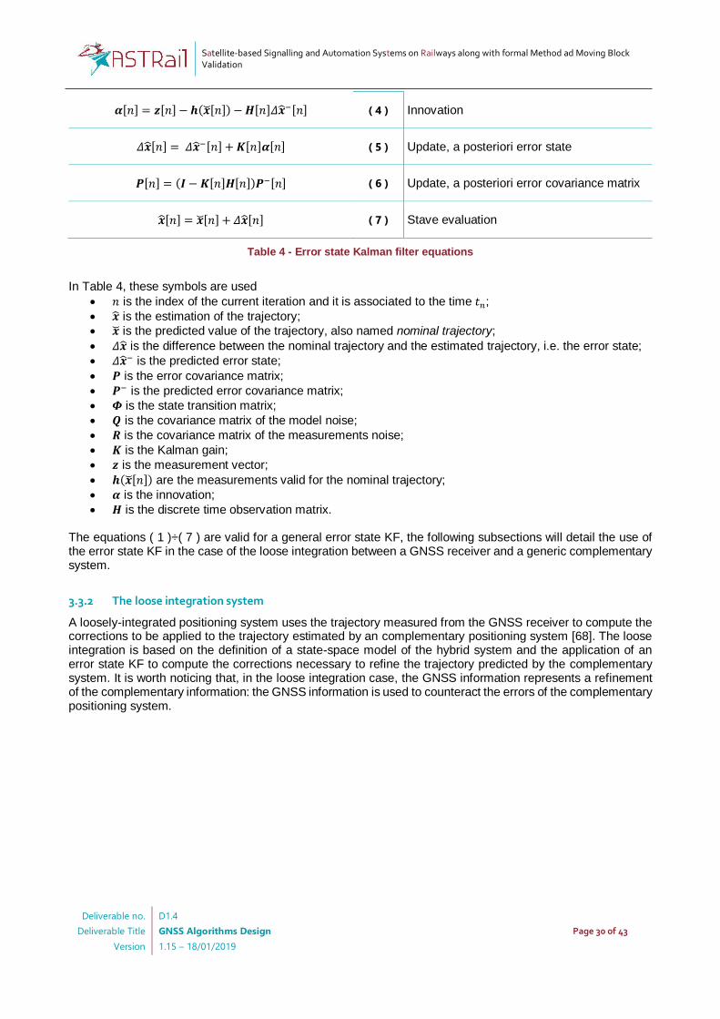
Satellite-based Signalling and Automation Systems on Railways along with formal Method ad Moving Block Validation
Deliverable no.
Deliverable Title
Version
D1.4
GNSS Algorithms Design
1.15 – 18/01/2019
Page 30 of 43
𝜶[𝑛] = 𝒛[𝑛] − 𝒉(𝒙[𝑛]) − 𝑯[𝑛]𝛥�̂�−[𝑛] ( 4 ) Innovation
𝛥�̂�[𝑛] = 𝛥�̂�−[𝑛] + 𝑲[𝑛]𝜶[𝑛] ( 5 ) Update, a posteriori error state
𝑷[𝑛] = (𝑰 − 𝑲[𝑛]𝑯[𝑛])𝑷−[𝑛] ( 6 ) Update, a posteriori error covariance matrix
�̂�[𝑛] = 𝒙[𝑛] + 𝛥�̂�[𝑛] ( 7 ) Stave evaluation
Table 4 - Error state Kalman filter equations
In Table 4, these symbols are used
𝑛 is the index of the current iteration and it is associated to the time 𝑡𝑛;
�̂� is the estimation of the trajectory;
𝒙 is the predicted value of the trajectory, also named nominal trajectory;
𝛥�̂� is the difference between the nominal trajectory and the estimated trajectory, i.e. the error state;
𝛥�̂�− is the predicted error state;
𝑷 is the error covariance matrix;
𝑷− is the predicted error covariance matrix;
𝜱 is the state transition matrix;
𝑸 is the covariance matrix of the model noise;
𝑹 is the covariance matrix of the measurements noise;
𝑲 is the Kalman gain;
𝒛 is the measurement vector;
𝒉(𝒙[𝑛]) are the measurements valid for the nominal trajectory;
𝜶 is the innovation;
𝑯 is the discrete time observation matrix. The equations ( 1 )÷( 7 ) are valid for a general error state KF, the following subsections will detail the use of the error state KF in the case of the loose integration between a GNSS receiver and a generic complementary system.
3.3.2 The loose integration system
A loosely-integrated positioning system uses the trajectory measured from the GNSS receiver to compute the corrections to be applied to the trajectory estimated by an complementary positioning system [68]. The loose integration is based on the definition of a state-space model of the hybrid system and the application of an error state KF to compute the corrections necessary to refine the trajectory predicted by the complementary system. It is worth noticing that, in the loose integration case, the GNSS information represents a refinement of the complementary information: the GNSS information is used to counteract the errors of the complementary positioning system.
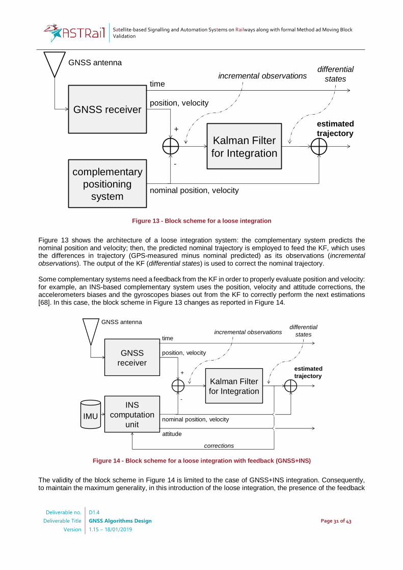
Satellite-based Signalling and Automation Systems on Railways along with formal Method ad Moving Block Validation
Deliverable no.
Deliverable Title
Version
D1.4
GNSS Algorithms Design
1.15 – 18/01/2019
Page 31 of 43
GNSS receiver
Kalman Filter
for Integration
complementary
positioning
system
position, velocity
nominal position, velocity
GNSS antenna
-
+
incremental observationsdifferential
statestime
estimated
trajectory
Figure 13 - Block scheme for a loose integration
Figure 13 shows the architecture of a loose integration system: the complementary system predicts the nominal position and velocity; then, the predicted nominal trajectory is employed to feed the KF, which uses the differences in trajectory (GPS-measured minus nominal predicted) as its observations (incremental observations). The output of the KF (differential states) is used to correct the nominal trajectory. Some complementary systems need a feedback from the KF in order to properly evaluate position and velocity: for example, an INS-based complementary system uses the position, velocity and attitude corrections, the accelerometers biases and the gyroscopes biases out from the KF to correctly perform the next estimations [68]. In this case, the block scheme in Figure 13 changes as reported in Figure 14.
GNSS
receiver
IMU
Kalman Filter
for Integration
INS
computation
unit
position, velocity
nominal position, velocity
GNSS antenna
-
+
incremental observationsdifferential
states
corrections
attitude
time
estimated
trajectory
Figure 14 - Block scheme for a loose integration with feedback (GNSS+INS)
The validity of the block scheme in Figure 14 is limited to the case of GNSS+INS integration. Consequently, to maintain the maximum generality, in this introduction of the loose integration, the presence of the feedback
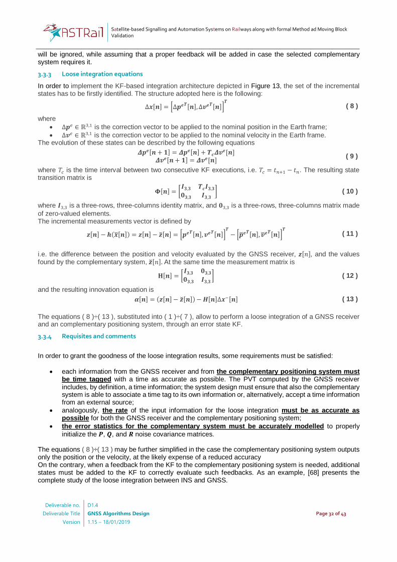
Satellite-based Signalling and Automation Systems on Railways along with formal Method ad Moving Block Validation
Deliverable no.
Deliverable Title
Version
D1.4
GNSS Algorithms Design
1.15 – 18/01/2019
Page 32 of 43
will be ignored, while assuming that a proper feedback will be added in case the selected complementary system requires it.
3.3.3 Loose integration equations
In order to implement the KF-based integration architecture depicted in Figure 13, the set of the incremental states has to be firstly identified. The structure adopted here is the following:
∆𝒙[𝒏] = [∆𝒑𝒆𝑻[𝒏], ∆𝒗𝒆𝑻[𝒏]]𝑻
( 8 )
where
∆𝒑𝑒 ∈ ℝ3,1 is the correction vector to be applied to the nominal position in the Earth frame;
∆𝒗𝑒 ∈ ℝ3,1 is the correction vector to be applied to the nominal velocity in the Earth frame. The evolution of these states can be described by the following equations
𝜟𝒑𝒆[𝒏 + 𝟏] = 𝜟𝒑𝒆[𝒏] + 𝑻𝒄𝜟𝒗𝒆[𝒏] 𝜟𝒗𝒆[𝒏 + 𝟏] = 𝜟𝒗𝒆[𝒏]
( 9 )
where 𝑇𝑐 is the time interval between two consecutive KF executions, i.e. 𝑇𝑐 = 𝑡𝑛+1 − 𝑡𝑛. The resulting state transition matrix is
𝚽[𝒏] = [𝑰𝟑,𝟑 𝑻𝒄𝑰𝟑,𝟑
𝟎𝟑,𝟑 𝑰𝟑,𝟑] ( 10 )
where 𝑰3,3 is a three-rows, three-columns identity matrix, and 𝟎3,3 is a three-rows, three-columns matrix made
of zero-valued elements. The incremental measurements vector is defined by
𝒛[𝒏] − 𝒉(𝒙[𝒏]) = 𝒛[𝒏] − �̆�[𝒏] = [𝒑𝒆𝑻[𝒏], 𝒗𝒆𝑻[𝒏]]𝑻
− [�̆�𝒆𝑻[𝒏], �̆�𝒆𝑻[𝒏]]𝑻
( 11 )
i.e. the difference between the position and velocity evaluated by the GNSS receiver, 𝒛[𝑛], and the values found by the complementary system, �̆�[𝑛]. At the same time the measurement matrix is
𝐇[𝒏] = [𝑰𝟑,𝟑 𝟎𝟑,𝟑
𝟎𝟑,𝟑 𝑰𝟑,𝟑] ( 12 )
and the resulting innovation equation is
𝜶[𝒏] = (𝒛[𝒏] − �̆�[𝒏]) − 𝑯[𝒏]∆𝒙−[𝒏] ( 13 )
The equations ( 8 )÷( 13 ), substituted into ( 1 )÷( 7 ), allow to perform a loose integration of a GNSS receiver and an complementary positioning system, through an error state KF.
3.3.4 Requisites and comments
In order to grant the goodness of the loose integration results, some requirements must be satisfied:
each information from the GNSS receiver and from the complementary positioning system must be time tagged with a time as accurate as possible. The PVT computed by the GNSS receiver includes, by definition, a time information; the system design must ensure that also the complementary system is able to associate a time tag to its own information or, alternatively, accept a time information from an external source;
analogously, the rate of the input information for the loose integration must be as accurate as possible for both the GNSS receiver and the complementary positioning system;
the error statistics for the complementary system must be accurately modelled to properly
initialize the 𝑷, 𝑸, and 𝑹 noise covariance matrices. The equations ( 8 )÷( 13 ) may be further simplified in the case the complementary positioning system outputs only the position or the velocity, at the likely expense of a reduced accuracy On the contrary, when a feedback from the KF to the complementary positioning system is needed, additional states must be added to the KF to correctly evaluate such feedbacks. As an example, [68] presents the complete study of the loose integration between INS and GNSS.
Satellite-based Signalling and Automation Systems on Railways along with formal Method ad Moving Block Validation
Deliverable no.
Deliverable Title
Version
D1.4
GNSS Algorithms Design
1.15 – 18/01/2019
Page 33 of 43
4 Algorithms for enhanced robustness against RFI (ISMB)
The contents of this section are part of the paper M. Troglia Gamba and E. Falletti, “Performance Analysis of FLL Schemes to Track Swept Jammers in an Adaptive Notch Filter” submitted to NAVITEC 2018
In [RD.1], four GNSS interference models have been selected as the most relevant for the railways domain: Continuous Wave (CW), NarrowBand (NB), WideBand (WB) and Swept interferences. In particular, the swept signal, also known as ‘chirp’, is the typical format of the jammers’ transmission. In this regard, among the intentional interferences, the jamming is a real threat and its occurrence has been witnessed in many recent newspaper and magazine articles [51]–[53]. Despite its purchase is illegal in most countries, a jamming device is cheap, easy to be found and easy to be used: it is sufficient to turn it on to see its effects, since it simply relies on power and spectral occupation to deny the GNSS signals. Simple jammers can disrupt GNSS-based services in wide geographical areas (even in several kilometers) [54]. Several techniques to detect, characterize and mitigate interfering signals, including jammers, has been investigated so far. A comprehensive performance analysis and comparison of the main state-of-art solutions can be found in [55]. Among all of these, the Adaptive Notch Filter (ANF) to counteract narrowband interference is still appealing for its ease of implementation, low computational cost and reduced activation time compared to other more effective but far computationally demanding solutions such as transform domain excision techniques [56]. ANFs are well-known to be particularly effective for CW interferes: much effort has been spent so far in investigating and improving its adaptation capability [57][58]. Representing a good compromise between efficiency and complexity, ANFs has proved to be an efficient mitigation technique also for NB [59]. After all, CW can be considered as a particular case of the NB. Moreover, a preliminary demonstration of the suitability of the ANF in mitigating also the effects of commercial GNSS jammers (swept) has been presented in [61], where a remarkable improvement in terms of carrier-to-noise ratio is shown in the receiver when the jammer is filtered out. Therefore, ANFs are definitely a versatile solution, able to detect and mitigate CW, NB and swept interfering signals. A separate discussion, instead, has to be deserved to WB interferers, which in most cases can only be detected, while their mitigation can actually be useless since a too wide bandwidth can really compromise the GNSS signal recover. According to this discussion, the ANF has been selected as a viable candidate to be adopted in a GNSS-centric architecture for the railways domain. In particular, a specific family of ANFs has been identified, as better detailed in the next subsection. The jamming classification and selection is reported in subsection 4.2, while the high-level description of the algorithm is illustrated in subsection 4.3. Finally, the key performance parameters to be used during the test phase are discussed in subsection 4.4.
4.1 Identification of the target algorithm: Frequency Lock Loop (FLL) – equivalent ANF
ANFs have been widely exploited in literature, with many variations. More recently, the equivalence between ANFs and Frequency Lock Loops (FLLs) has been analytically demonstrated [66]. In particular, two FLL equivalent models of ANF are considered, according to the Plain Gradient (PG) rule employed in the adaptation algorithm: the standard FLL and the exponential filtering FLL [60]. Such an equivalence is particularly interesting, since FLL theory, widely employed in GNSS tracking loop analysis, can then be used to characterize the adaptive performance of the ANF. The analysis conducted in [66] is limited to CW interfering signals, while the behaviour of FLL-based ANFs in case of swept interferers has not been fully explored yet. We started from both FLL models of ANF introduced in [66] to conduct a performance evaluation in case of jamming (swept) interferers. In particular, the exponential FLL, albeit able to track narrow swept jamming signals, proves to not be suitable for more challenging jamming signals with very fast frequency variations. For this reason, we investigated the standard FLL ANF as a viable alternative, showing better performance.
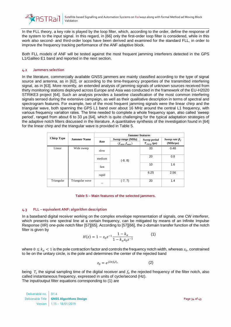
Satellite-based Signalling and Automation Systems on Railways along with formal Method ad Moving Block Validation
Deliverable no.
Deliverable Title
Version
D1.4
GNSS Algorithms Design
1.15 – 18/01/2019
Page 34 of 43
In the FLL theory, a key role is played by the loop filter, which, according to the order, define the response of the system to the input signal. In this regard, in [66] only the first-order loop filter is considered, while in this work also second- and third-order loops have been derived and examined for the standard FLL, in order to improve the frequency tracking performance of the ANF adaptive block. Both FLL models of ANF will be tested against the most frequent jamming interferers detected in the GPS L1/Galileo E1 band and reported in the next section.
4.2 Jammers selection
In the literature, commercially available GNSS jammers are mainly classified according to the type of signal source and antenna, as in [62], or according to the time-frequency properties of the transmitted interfering signal, as in [63]. More recently, an extended analysis of jamming signals of unknown sources received from thirty monitoring stations deployed across Europe and Asia was conducted in the framework of the EU-H2020 STRIKE3 project [64]. Such an analysis provides a baseline classification of the most common interfering signals sensed during the extensive campaign, as well as their qualitative description in terms of spectral and spectrogram features. For example, two of the most frequent jamming signals were the linear chirp and the triangular wave, both spanning the GPS L1 band over about 16 MHz around the central L1 frequency, with various frequency variation rates. The time needed to complete a whole frequency span, also called ‘sweep period’, ranged from about 6 to 33 μs [64], which is quite challenging for the typical adaptation strategies of the adaptive notch filters discussed in the literature. A quantitative synthesis of the investigation found in [64] for the linear chirp and the triangular wave is provided in Table 5.
Chirp Type Jammer Name
Jammer features
Rate Sweep range (MHz) Sweep period
𝑻𝒄𝒉𝒊𝒓𝒑 (µs)
Sweep rate 𝜷𝒇
(MHz/µs) (𝒇𝒎𝒊𝒏, 𝒇𝒎𝒂𝒙)
Linear Wide sweep slow
(-8, 8)
33 0.48
medium 20 0.8
fast 10 1.6
rapid 6.25 2.56
Triangular Triangular wave --
(-7, 7) 20 1.4
Table 5 – Main features of the selected jammers.
4.3 FLL – equivalent ANF: algorithm description
In a baseband digital receiver working on the complex envelope representation of signals, one CW interferer, which presents one spectral line at a certain frequency, can be mitigated by means of an Infinite Impulse Response (IIR) one-pole notch filter [57][65]. According to [57][66], the z-domain transfer function of the notch filter is given by
𝐻(𝑧) = 1 − 𝑧0𝑧−11 − 𝑘𝛼
1 − 𝑘𝛼𝑧0𝑧−1
(1)
where 0 ≤ 𝑘𝛼 < 1 is the pole contraction factor and controls the frequency notch width, whereas 𝑧0, constrained to lie on the unitary circle, is the pole and determines the center of the rejected band
𝑧0 = 𝑒𝑗2𝜋𝑓0𝑇𝑠 (2)
being 𝑇𝑠 the signal sampling time of the digital receiver and 𝑓0 the rejected frequency of the filter notch, also called instantaneous frequency, expressed in units of cycle/second (Hz). The input/output filter equations corresponding to (1) are
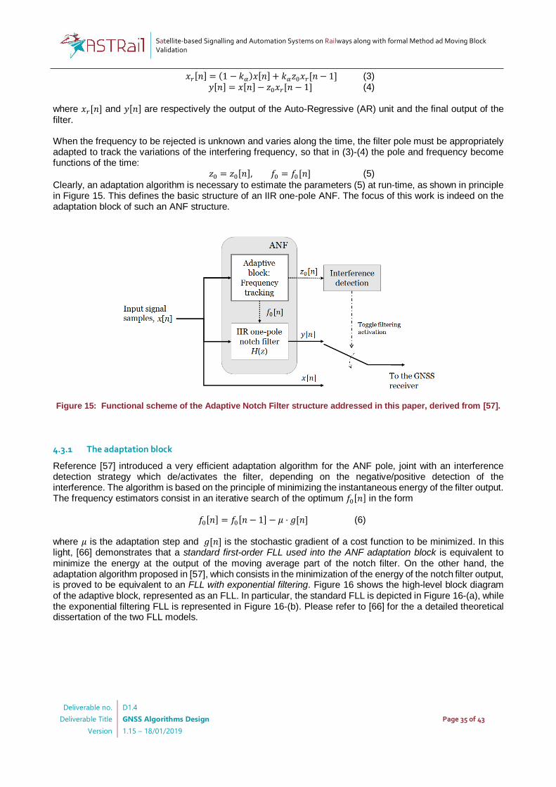
Satellite-based Signalling and Automation Systems on Railways along with formal Method ad Moving Block Validation
Deliverable no.
Deliverable Title
Version
D1.4
GNSS Algorithms Design
1.15 – 18/01/2019
Page 35 of 43
𝑥𝑟[𝑛] = (1 − 𝑘𝛼)𝑥[𝑛] + 𝑘𝛼𝑧0𝑥𝑟[𝑛 − 1] (3) 𝑦[𝑛] = 𝑥[𝑛] − 𝑧0𝑥𝑟[𝑛 − 1] (4)
where 𝑥𝑟[𝑛] and 𝑦[𝑛] are respectively the output of the Auto-Regressive (AR) unit and the final output of the filter. When the frequency to be rejected is unknown and varies along the time, the filter pole must be appropriately adapted to track the variations of the interfering frequency, so that in (3)-(4) the pole and frequency become functions of the time:
𝑧0 = 𝑧0[𝑛], 𝑓0 = 𝑓0[𝑛] (5)
Clearly, an adaptation algorithm is necessary to estimate the parameters (5) at run-time, as shown in principle in Figure 15. This defines the basic structure of an IIR one-pole ANF. The focus of this work is indeed on the adaptation block of such an ANF structure.
Figure 15: Functional scheme of the Adaptive Notch Filter structure addressed in this paper, derived from [57].
4.3.1 The adaptation block
Reference [57] introduced a very efficient adaptation algorithm for the ANF pole, joint with an interference detection strategy which de/activates the filter, depending on the negative/positive detection of the interference. The algorithm is based on the principle of minimizing the instantaneous energy of the filter output. The frequency estimators consist in an iterative search of the optimum 𝑓0[𝑛] in the form
𝑓0[𝑛] = 𝑓0[𝑛 − 1] − 𝜇 ⋅ 𝑔[𝑛] (6) where 𝜇 is the adaptation step and 𝑔[𝑛] is the stochastic gradient of a cost function to be minimized. In this light, [66] demonstrates that a standard first-order FLL used into the ANF adaptation block is equivalent to minimize the energy at the output of the moving average part of the notch filter. On the other hand, the adaptation algorithm proposed in [57], which consists in the minimization of the energy of the notch filter output, is proved to be equivalent to an FLL with exponential filtering. Figure 16 shows the high-level block diagram of the adaptive block, represented as an FLL. In particular, the standard FLL is depicted in Figure 16-(a), while the exponential filtering FLL is represented in Figure 16-(b). Please refer to [66] for the a detailed theoretical dissertation of the two FLL models.
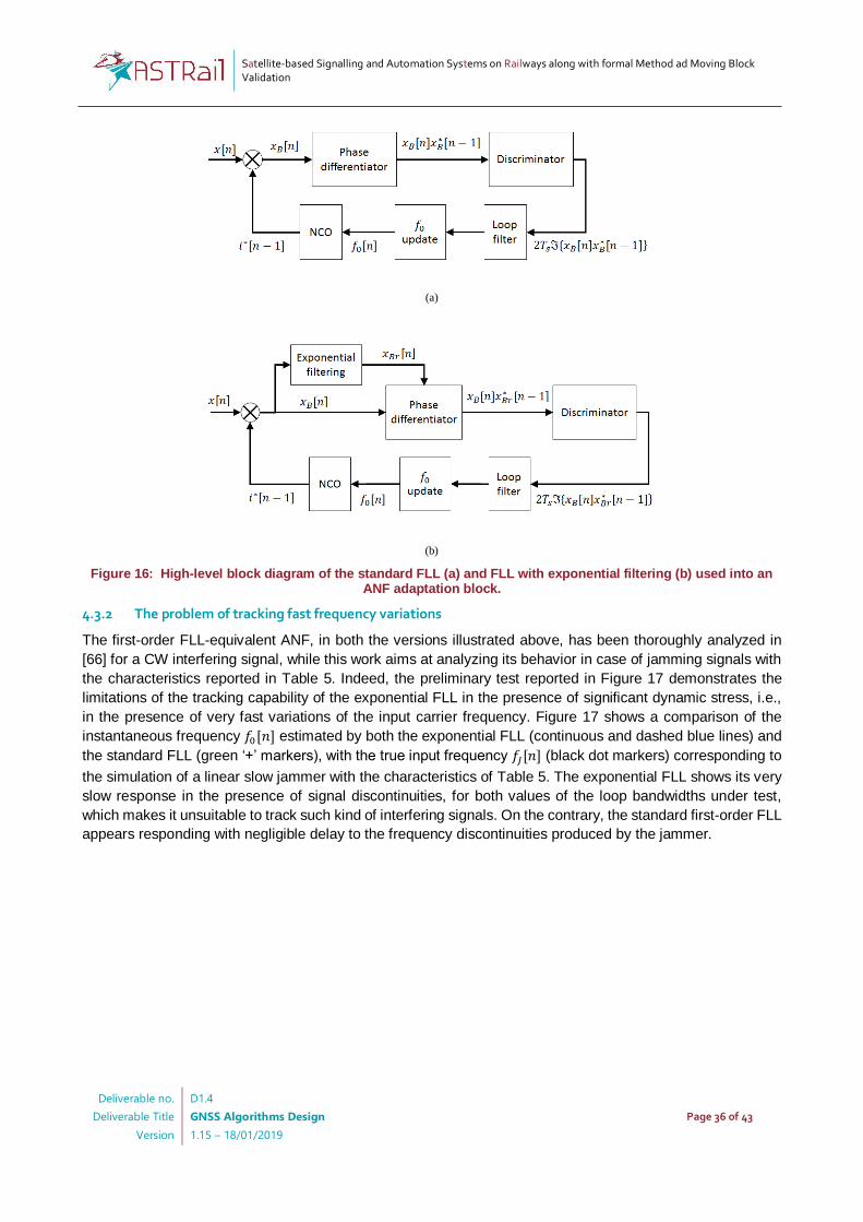
Satellite-based Signalling and Automation Systems on Railways along with formal Method ad Moving Block Validation
Deliverable no.
Deliverable Title
Version
D1.4
GNSS Algorithms Design
1.15 – 18/01/2019
Page 36 of 43
(a)
(b)
Figure 16: High-level block diagram of the standard FLL (a) and FLL with exponential filtering (b) used into an ANF adaptation block.
4.3.2 The problem of tracking fast frequency variations
The first-order FLL-equivalent ANF, in both the versions illustrated above, has been thoroughly analyzed in
[66] for a CW interfering signal, while this work aims at analyzing its behavior in case of jamming signals with
the characteristics reported in Table 5. Indeed, the preliminary test reported in Figure 17 demonstrates the
limitations of the tracking capability of the exponential FLL in the presence of significant dynamic stress, i.e.,
in the presence of very fast variations of the input carrier frequency. Figure 17 shows a comparison of the
instantaneous frequency 𝑓0[𝑛] estimated by both the exponential FLL (continuous and dashed blue lines) and
the standard FLL (green ‘+’ markers), with the true input frequency 𝑓𝐽[𝑛] (black dot markers) corresponding to
the simulation of a linear slow jammer with the characteristics of Table 5. The exponential FLL shows its very
slow response in the presence of signal discontinuities, for both values of the loop bandwidths under test,
which makes it unsuitable to track such kind of interfering signals. On the contrary, the standard first-order FLL
appears responding with negligible delay to the frequency discontinuities produced by the jammer.
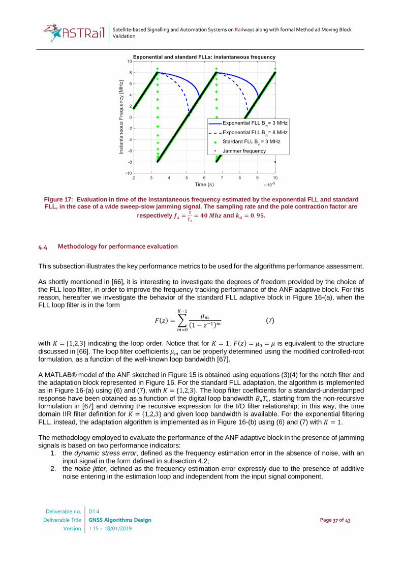
Satellite-based Signalling and Automation Systems on Railways along with formal Method ad Moving Block Validation
Deliverable no.
Deliverable Title
Version
D1.4
GNSS Algorithms Design
1.15 – 18/01/2019
Page 37 of 43
Figure 17: Evaluation in time of the instantaneous frequency estimated by the exponential FLL and standard FLL, in the case of a wide sweep-slow jamming signal. The sampling rate and the pole contraction factor are
respectively 𝒇𝒔 =𝟏
𝑻𝒔= 𝟒𝟎 𝑴𝒉𝒛 and 𝒌𝜶 = 𝟎. 𝟗𝟓.
4.4 Methodology for performance evaluation
This subsection illustrates the key performance metrics to be used for the algorithms performance assessment. As shortly mentioned in [66], it is interesting to investigate the degrees of freedom provided by the choice of the FLL loop filter, in order to improve the frequency tracking performance of the ANF adaptive block. For this reason, hereafter we investigate the behavior of the standard FLL adaptive block in Figure 16-(a), when the FLL loop filter is in the form
𝐹(𝑧) = ∑𝜇𝑚
(1 − 𝑧−1)𝑚
𝐾−1
𝑚=0
(7)
with 𝐾 = {1,2,3} indicating the loop order. Notice that for 𝐾 = 1, 𝐹(𝑧) = 𝜇0 = 𝜇 is equivalent to the structure
discussed in [66]. The loop filter coefficients 𝜇𝑚 can be properly determined using the modified controlled-root formulation, as a function of the well-known loop bandwidth [67]. A MATLAB® model of the ANF sketched in Figure 15 is obtained using equations (3)(4) for the notch filter and the adaptation block represented in Figure 16. For the standard FLL adaptation, the algorithm is implemented as in Figure 16-(a) using (6) and (7), with 𝐾 = {1,2,3}. The loop filter coefficients for a standard-underdamped response have been obtained as a function of the digital loop bandwidth 𝐵𝑛𝑇𝑠, starting from the non-recursive formulation in [67] and deriving the recursive expression for the I/O filter relationship; in this way, the time domain IIR filter definition for 𝐾 = {1,2,3} and given loop bandwidth is available. For the exponential filtering
FLL, instead, the adaptation algorithm is implemented as in Figure 16-(b) using (6) and (7) with 𝐾 = 1. The methodology employed to evaluate the performance of the ANF adaptive block in the presence of jamming signals is based on two performance indicators:
1. the dynamic stress error, defined as the frequency estimation error in the absence of noise, with an input signal in the form defined in subsection 4.2;
2. the noise jitter, defined as the frequency estimation error expressly due to the presence of additive noise entering in the estimation loop and independent from the input signal component.
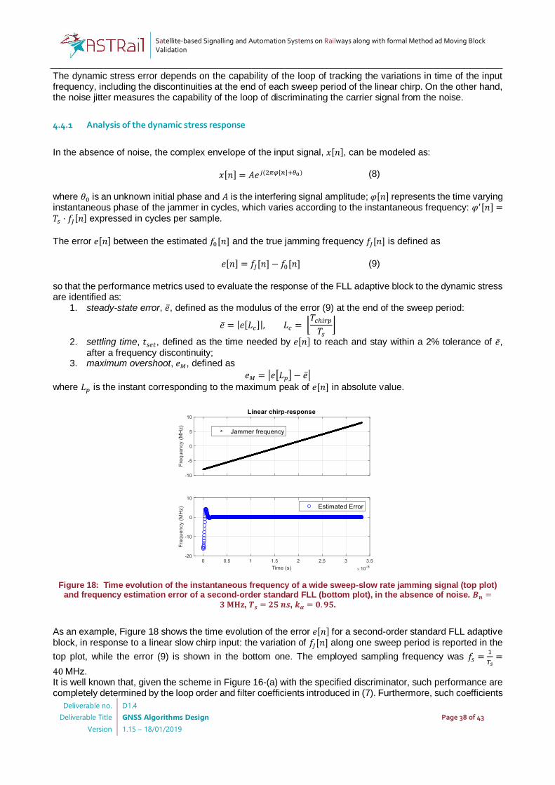
Satellite-based Signalling and Automation Systems on Railways along with formal Method ad Moving Block Validation
Deliverable no.
Deliverable Title
Version
D1.4
GNSS Algorithms Design
1.15 – 18/01/2019
Page 38 of 43
The dynamic stress error depends on the capability of the loop of tracking the variations in time of the input frequency, including the discontinuities at the end of each sweep period of the linear chirp. On the other hand, the noise jitter measures the capability of the loop of discriminating the carrier signal from the noise.
4.4.1 Analysis of the dynamic stress response
In the absence of noise, the complex envelope of the input signal, 𝑥[𝑛], can be modeled as:
𝑥[𝑛] = 𝐴𝑒𝑗(2𝜋𝜑[𝑛]+𝜃0) (8)
where 𝜃0 is an unknown initial phase and 𝐴 is the interfering signal amplitude; 𝜑[𝑛] represents the time varying instantaneous phase of the jammer in cycles, which varies according to the instantaneous frequency: 𝜑′[𝑛] =𝑇𝑠 ⋅ 𝑓𝐽[𝑛] expressed in cycles per sample.
The error 𝑒[𝑛] between the estimated 𝑓0[𝑛] and the true jamming frequency 𝑓𝐽[𝑛] is defined as
𝑒[𝑛] = 𝑓𝐽[𝑛] − 𝑓0[𝑛] (9)
so that the performance metrics used to evaluate the response of the FLL adaptive block to the dynamic stress are identified as:
1. steady-state error, �̅�, defined as the modulus of the error (9) at the end of the sweep period:
�̅� = |𝑒[𝐿𝑐]|, 𝐿𝑐 = ⌊𝑇𝑐ℎ𝑖𝑟𝑝
𝑇𝑠
⌋
2. settling time, 𝑡𝑠𝑒𝑡, defined as the time needed by 𝑒[𝑛] to reach and stay within a 2% tolerance of �̅�, after a frequency discontinuity;
3. maximum overshoot, 𝑒𝑀, defined as
𝑒𝑀 = |𝑒[𝐿𝑝] − �̅�|
where 𝐿𝑝 is the instant corresponding to the maximum peak of 𝑒[𝑛] in absolute value.
Figure 18: Time evolution of the instantaneous frequency of a wide sweep-slow rate jamming signal (top plot) and frequency estimation error of a second-order standard FLL (bottom plot), in the absence of noise. 𝑩𝒏 =
𝟑 𝐌𝐇𝐳, 𝑻𝒔 = 𝟐𝟓 𝒏𝒔, 𝒌𝜶 = 𝟎. 𝟗𝟓.
As an example, Figure 18 shows the time evolution of the error 𝑒[𝑛] for a second-order standard FLL adaptive block, in response to a linear slow chirp input: the variation of 𝑓𝐽[𝑛] along one sweep period is reported in the
top plot, while the error (9) is shown in the bottom one. The employed sampling frequency was 𝑓𝑠 =1
𝑇𝑠=
40 MHz. It is well known that, given the scheme in Figure 16-(a) with the specified discriminator, such performance are completely determined by the loop order and filter coefficients introduced in (7). Furthermore, such coefficients
Satellite-based Signalling and Automation Systems on Railways along with formal Method ad Moving Block Validation
Deliverable no.
Deliverable Title
Version
D1.4
GNSS Algorithms Design
1.15 – 18/01/2019
Page 39 of 43
also determine the frequency-domain characteristics of the loop, described by the so-called loop bandwidth
𝐵𝑛. Indeed, [67] provides the explicit relationship between values of the loop bandwidth and corresponding sets of loop filter coefficients {𝜇𝑚}, for a standard digital phase lock loop and various orders 𝐾. For this reason,
the analysis is conducted as a function of 𝐵𝑛. Different loop orders and input signals are also evaluated.
4.4.2 Analysis of the noise jitter
In the presence of noise, (8) becomes:
𝑥[𝑛] = 𝐴𝑒𝑗(2𝜋𝜑[𝑛]+𝜃0) + 𝑤[𝑛] (10)
where 𝑤[𝑛] is a complex Additive White Gaussian Noise (AWGN) process with zero mean and total variance
𝜎𝑤2 , identically distributed between the real and imaginary parts. 𝑤[𝑛] is statistically independent from the
deterministic input component (8) and therefore is analyzed separately. The frequency jitter is the component of the error 𝑒[𝑛] in (9), determined by the input component 𝑤[𝑛]. In lock conditions, the loop can be approximately considered a linear system, then the noise inside the loop maintains its zero mean and Gaussian properties: therefore, its impact can be completely quantified by means of its
variance metric: 𝜎𝑓2. Since the noise filtering properties of the loop are a function of the filter coefficients through
the loop bandwidth again, then the noise jitter analysis is conducted as a function of 𝐵𝑛 and filter order 𝐾 ={1,2,3}, for several values of Interference-to-Noise Ratio (INR) conditions. Based on the above described key metrics, the performance evaluation in terms of dynamic stress response and noise jitter will be conducted and included in the next deliverable [RD.3].
5 Conclusions (ISMB-NavSAS)
This document presented the definition of a GNSS-centric architecture suitable for positioning in rail safety applications, and the selection and design of possible algorithms to enhance the positioning availability and the RFI resilience. In particular, a multi-sensor Virtual Balise reader GNSS-based train positioning system to be integrated to the current ERTMS/ETCS has been proposed and outlined. Three main operational scenarios affected by reduced visibility issues have been identified: in station, in tunnel and in proximity of railway exchanges. In order to improve positioning availability in such scenarios, three main categories of GNSS complementary technologies have been considered: wireless, visual-based and dead-reckoning methods. Thus, a discussion on possible integration approaches has been addressed and a feasible loose-coupling architecture has been also proposed. Finally, after a state-of-art scouting on RFI detection and mitigation techniques, the ANF has been selected as a versatile and low-complexity solution, able to remove CW, NB and swept interferers. Among all the variations available in literature, the FLL-equivalent ANF is particularly interesting, allowing the use of the FLL theory to analyse its behaviour. Two models of FLL-equivalent ANF have been considered: the standard FLL and the exponential filtering FLL. While the latter seems not being able to track very fast frequency changes, as shown from preliminary results, the former exhibits much better performance, responding with negligible delay to the frequency discontinuities, which typically characterize jamming signals. For this reason, the standard FLL ANF has been investigated as a more suitable solution. The algorithm description and design of both models has been provided and key performance indicators to be used for the performance evaluation have been also derived.
Satellite-based Signalling and Automation Systems on Railways along with formal Method ad Moving Block Validation
Deliverable no.
Deliverable Title
Version
D1.4
GNSS Algorithms Design
1.15 – 18/01/2019
Page 40 of 43
List of figures
Figure 1 – Reference architecture for VB concept ................................................................................................................................................... 6
Figure 2: Odometry Diagnostic Test Software Architecture .............................................................................................................................. 11
Figure 3: Slipping Errors [23] ........................................................................................................................................................................................... 13
Figure 4: Sliding Errors [23].............................................................................................................................................................................................. 14
Figure 5: Wheel slipping Tachometer Errors [21] ................................................................................................................................................... 14
Figure 6: Wheel Speed Estimates using Tachometer and reference [19] ..................................................................................................... 15
Figure 7: Fault Diagnosis Monitor Bank ..................................................................................................................................................................... 16
Figure 8: Monitor Histograms ........................................................................................................................................................................................ 16
Figure 9: Threshold Definition ........................................................................................................................................................................................ 17
Figure 10: Probability of No Detection vs. Detection Time ................................................................................................................................ 18
Figure 11: Probability of Missed Detection vs. Detection Time ....................................................................................................................... 19
Figure 12: Expected Detection Times .......................................................................................................................................................................... 20
Figure 13 - Block scheme for a loose integration .................................................................................................................................................. 31
Figure 14 - Block scheme for a loose integration with feedback (GNSS+INS) .......................................................................................... 31
Figure 15: Functional scheme of the Adaptive Notch Filter structure addressed in this paper, derived from [57]. ................. 35
Figure 16: High-level block diagram of the standard FLL (a) and FLL with exponential filtering (b) used into an ANF
adaptation block. ................................................................................................................................................................................................................. 36
Figure 17: Evaluation in time of the instantaneous frequency estimated by the exponential FLL and standard FLL, in the
case of a wide sweep-slow jamming signal. The sampling rate and the pole contraction factor are respectively 𝒇𝒔 = 𝟏𝑻𝒔 =
𝟒𝟎 𝑴𝒉𝒛 and 𝒌𝜶 = 𝟎. 𝟗𝟓. ................................................................................................................................................................................................... 37
Figure 18: Time evolution of the instantaneous frequency of a wide sweep-slow rate jamming signal (top plot) and
frequency estimation error of a second-order standard FLL (bottom plot), in the absence of noise. 𝑩𝒏 = 𝟑 𝐌𝐇𝐳, 𝑻𝒔 =
𝟐𝟓 𝒏𝒔, 𝒌𝜶 = 𝟎. 𝟗𝟓. ............................................................................................................................................................................................................... 38
List of tables
Table 1: Input Parameters .................................................................................................................................................................................................. 7
Table 2: Failures .................................................................................................................................................................................................................... 15
Table 3 – Target operational scenarios....................................................................................................................................................................... 21
Table 4 - Error state Kalman filter equations ........................................................................................................................................................... 30
Table 5 – Main features of the selected jammers. ................................................................................................................................................. 34
References
[1] EU-H2020 Shift2Rail (S2R) project, Available online: https://shift2rail.org/ (accessed on 10 July 2018)
[2] C. Wullems, “Safety Analysis Part 1 – Functional Analysis,” Funct. Anal., p. 37.
[3] WG-C, “EU-US Cooperation on Satellite Navigation Working Group C ARAIM Technical Subgroup Milestone Report 3.”
Feb-2016.
[4] M. Brenner and F. Liu, “Ranging Source Fault Detection Performance for Category III GBAS,” in ION GNSS, 2010.
[5] B. Roturier, E. Chatre, and J. Ventura-Travesat, “The SBAS Integrity Concept Standardised by. ESA,” 2001.
[6] A. Filip, “TRAVELLING VIRTUAL BALISE FOR ETCS,” WIT Trans. State---Art Sci. Eng., vol. 1, pp. 272–282, Dec. 2016.
[7] T. R. Schempp, S. R. Peck, and R. M. Fries, “WAAS Algorithm Contribution to Hazardously Misleading Information (HMI),”
p. 7, 2001.
[8] J. Blanch, “Advanced RAIM User Algorithm Description: Integrity Support Message Processing, Fault Detection, Exclusion
and Protection Level Calculation,” in Proceedings of ION GNSS, 2012.
Satellite-based Signalling and Automation Systems on Railways along with formal Method ad Moving Block Validation
Deliverable no.
Deliverable Title
Version
D1.4
GNSS Algorithms Design
1.15 – 18/01/2019
Page 41 of 43
[9] C. Wullems, “Safety Analysis Part 3 – Assessment of the Virtual Balise Subsystem for THR Apportionment,” p. 47.
[10] J. Blanch et al., “Baseline advanced RAIM user algorithm and possible improvements,” IEEE Trans. Aerosp. Electron. Syst.,
vol. 51, no. 1, pp. 713–732, Jan. 2015.
[11] S. Peck and J. Tekawy, “User Differential Range Error Algorithms for the Wide Area Augmentation System,” p. 9.
[12] W. Werner, U. Rossbach, and R. Wolf, “Algorithms and Performance of the EGNOS CPF Independent Check Set,” p. 11.
[13] J. T. Wu and S. Peck, “An Analysis of Satellite Integrity Monitoring Improvement for WAAS,” p. 10, 2002.
[14] A. Filip, “Efficient use of multi-constellation EGNOS for the European Train Control System,” in ENC GNSS 2016, 2016.
[15] UNISIG, “Safety Requirements for the Technical Interoperability of ECTS in Levels 1 and 2.” .
[16] RTCA, “Mininum Operational Performance Standards for Global Positioning System/Wide Area augmentation System
Airborne Equipment - DO-229D.” 2006.
[17] DoD/DoT, “GPS Standard Positioning Service (SPS)Performance Standard.” 2008.
[18] P. Brocard, “Integrity Monioring for mobile users in urban environment,” INPT, Toulouse, 2016.
[19] B. Allotta, V. Colla, and M. Malvezzi, “Train position and speed estimation using wheel velocity measurements,” Proc. Inst.
Mech. Eng. Part F J. Rail Rapid Transit, vol. 216, no. 3, pp. 207–225, May 2002.
[20] D. Kellner, M. Barjenbruch, K. Dietmayer, J. Klappstein, and J. Dickmann, “Joint Radar Alignment and Odometry
Calibration,” p. 10.
[21] A. W. Palmer and N. Nourani-Vatani, “Robust Odometry using Sensor Consensus Analysis,” ArXiv180302237 Cs, Mar. 2018.
[22] B. Allotta, L. Pugi, A. Ridolfi, M. Malvezzi, G. Vettori, and A. Rindi, “Evaluation of odometry algorithm performances using
a railway vehicle dynamic model,” Veh. Syst. Dyn., vol. 50, no. 5, pp. 699–724, May 2012.
[23] A. Neri, S. Sabina, and U. Mascia, “GNSS and Odometry Fusion for High Integrity and High Availability Train Control
Systems,” p. 10.
[24] B. Allotta et al., “An innovative localisation algorithm for railway vehicles,” Veh. Syst. Dyn., vol. 52, no. 11, pp. 1443–1469,
Nov. 2014.
[25] Campos, Rafael Saraiva. “Evolution of positioning techniques in cellular networks, from 2G to 4G”, Wireless
Communications and Mobile Computing 2017 (2017).
[26] Tippe, Yogesh S., and Pramila S. Shinde, “Mobile Positioning in Cellular Networks”, IJTRD, Sep-Oct 2016.
[27] S. Fischer, “Introduction to OTDOA on LTE Networks”, Qualcomm Technologies, Inc (2014): 1-18.
[28] A. Roessler, M. Kottkamp, “LTE-Advanced (3GPP Rel. 11) Technology Introduction White Paper”, White Paper -
1MA232_1E, Rohde & Schwarz International (2013).
[29] S. Fischer, “Observed time difference of arrival (OTDOA) positioning in 3GPP LTE”, Qualcomm White Pap 1.1 (2014): 1-
62.
[30] Elbahhar, Fouzia, and Marc Heddebaut. "Advanced Train Positioning/Communication System." Modern Railway
Engineering. InTech, 2018.
[31] Koyuncu, Hakan, and Shuang Hua Yang. "A survey of indoor positioning and object locating systems." IJCSNS
International Journal of Computer Science and Network Security 10.5 (2010): 121-128.
[32] Soganci, Hamza, Sinan Gezici, and H. Vincent Poor. "Accurate positioning in ultra-wideband systems." IEEE Wireless
Communications 18.2 (2011).
[33] Alarifi, Abdulrahman, et al. "Ultra wideband indoor positioning technologies: Analysis and recent advances." Sensors 16.5
(2016): 707.
[34] ETSI, TR 101 538, “UWB location tracking devices in the railroad environment”, European Telecommunications Standards
Institute (2012).
[35] Huang, J., Presti, L. L., Garello, R., & Sacco, B. (2012, August). Study of positioning methods in DVB-T single frequency
networks. In Communications and Electronics (ICCE), 2012 Fourth International Conference on (pp. 263-268). IEEE.
[36] Huang, J., Lo Presti, L., & Garello, R. (2013). Digital video broadcast-terrestrial (DVB-T) single frequency networks
positioning in dynamic scenarios. Sensors, 13(8), 10191-10218.
[37] Chen, L., Julien, O., Thevenon, P., Serant, D., Peña, A. G., & Kuusniemi, H. (2015). TOA estimation for positioning with
DVB-T signals in outdoor static tests. IEEE Transactions on Broadcasting, 61(4), 625-638.
[38] Ben-Afia, Amani, et al. "Review and classification of vision-based localisation techniques in unknown environments." IET
Radar, Sonar & Navigation 8.9 (2014): 1059-1072.
[39] Aqel, Mohammad OA, et al. "Review of visual odometry: types, approaches, challenges, and applications." SpringerPlus
5.1 (2016): 1897.
[40] Viulib® SDK - Vicomtech, “Real-time accurate egomotion estimation for trains using optical flow”,
http://www.viulib.org/solutions/s6/accurate_egomotion, visited July 2018

Satellite-based Signalling and Automation Systems on Railways along with formal Method ad Moving Block Validation
Deliverable no.
Deliverable Title
Version
D1.4
GNSS Algorithms Design
1.15 – 18/01/2019
Page 42 of 43
[41] Reliable Data Systems International Ltd, “Video Train Positioning System”, http://www.rdsintl.com/train-positioning-
system/2-video-train-positioning-system/ , visited July 2018
[42] Wohlfeil, J. (2011, June). Vision based rail track and switch recognition for self-localization of trains in a rail network. In
Intelligent Vehicles Symposium (IV), 2011 IEEE (pp. 1025-1030). IEEE.
[43] Resendiz, E., Molina, L. F., Hart, J. M., Edwards, J. R., Sawadisavi, S., Ahuja, N., & Barkan, C. P. L. (2010, July). Development
of a machine-vision system for inspection of railway track components. In 12th World Conference on Transport Research,
Lisbon, Portugal.
[44] Aminmansour, S., Maire, F., & Wullems, C. (2014, November). Near-miss event detection at railway level crossings. In
Digital lmage Computing: Techniques and Applications (DlCTA), 2014 International Conference on (pp. 1-8). IEEE.
[45] ERTMS/ETCS – Class 1 – Performance Requirements for Interoperability, Subset-041 v3.1.0
[46] Neri, A., Sabina, S., Rispoli, F., & Mascia, U. (2015). GNSS and odometry fusion for high integrity and high availability train
control systems. ION GNSS+ 2015.
[47] Adin, I., Mendizabal, J., De Miguel, G., Goya, J., Zamora, L., & Arrizabalaga, S. (2016). Complementary positioning system
in GNSS-denied areas. Transportation Research Procedia, 14, 4562-4571.
[48] Heirich, O. (2016). Bayesian train localization with particle filter, loosely coupled GNSS, IMU, and a track map. Journal of
Sensors, 2016.
[49] Malvezzi, M., Allotta, B., & Rinchi, M. (2011). Odometric estimation for automatic train protection and control systems.
Vehicle system dynamics, 49(5), 723-739.
[50] Larsson, Martin. "Sensor fusion application to railway odometry." (2014).
[51] T. Rogoway, USAF Is Jamming GPS In The Western U.S. For Largest Ever Red Flag Air War Exercise, The Drive Magazine,
January 25, 2018. Available online: http://www.thedrive.com/the-war-zone/17987/usaf-is-jamming-gps-in-the-western-u-
s-for-largest-ever-red-flag-air-war-exercise (accessed on 11 June 2018).
[52] G. Nott, Qld cops aim high with signal jamming drone guns, CIO Magazine, 28 February, 2018. Available online:
https://www.cio.com.au/article/634011/qld-cops-aim-high-signal-jamming-drone-guns/ (accessed on 11 June 2018).
[53] Military Drones Prove Vulnerable to GPS Jamming, The Maritime Executive Magazine, 10 April, 2018. Available online:
https://www.maritime-executive.com/editorials/military-hardware-proves-vulnerable-to-gps-jamming#gs.=rDzJx0
(accessed on 11 June 2018).
[54] J. T. Curran, M. Bavaro, P. Closas and M. Navarro, A Look at the Threat of Systematic Jamming of GNSS, Sep/Oct issue,
2017.
[55] N. Fadaei, Detection, Characterization and Mitigation of GNSS Jamming Interference Using Pre-Correlation Methods,
Master of Science Thesis, Calgary , Alberta, April 2016
[56] M. G. Amin, D. Borio, Y. D. Zhang and L. Galleani, "Time-Frequency Analysis for GNSSs: From interference mitigation to
system monitoring," in IEEE Signal Processing Magazine, vol. 34, no. 5, pp. 85-95, Sept. 2017. doi:
10.1109/MSP.2017.2710235
[57] Borio, D.; Camoriano, L.; Lo Presti, L., “Two-Pole and Multi-Pole Notch Filters: A Computationally Effective Solution for
GNSS Interference Detection and Mitigation,” IEEE Systems Journal, Volume: 2, Issue: 1, Page(s): 38-47, 2008.
[58] M. Troglia Gamba, E. Falletti, D. Rovelli, and A. Tuozzi, “FPGA Implementation Issues of a Two-pole Adaptive Notch Filter
for GPS/Galileo Receivers,” in Proceedings of the 25th International Technical Meeting of The Satellite Division of the
Institute of Navigation (ION GNSS 2012), Nashville, TN, 2012, pp. 3549–3557.
[59] T. T. Nguyen, V. L. The, T. H. Ta, H. L. T. Nguyen, B. Motella, ”An Adaptive Bandwidth Notch Filter for GNSS Narrowband
Interference Mitigation”, Journal on Electronics and Communications, Vol. 4, No. 3–4, July–December, 2014
[60] Borio, D., Sokolova, N., Lachapelle, G.: ‘Memory discriminators for non-coherent integration in GNSS tracking loops’.
Proc. European Navigation Conf. (ENC), Naples, Italy, May 2009, pp. 1–12
[61] D. Borio, C. O'Driscoll and J. Fortuny, "GNSS Jammers: Effects and countermeasures," 2012 6th ESA Workshop on Satellite
Navigation Technologies (Navitec 2012) & European Workshop on GNSS Signals and Signal Processing, Noordwijk, 2012,
pp. 1-7. doi: 10.1109/NAVITEC.2012.6423048
[62] Mitch, Ryan H., Dougherty, Ryan C., Psiaki, Mark L., Powell, Steven P., O'Hanlon, Brady W., Bhatti, Jahshan A.,
Humphreys, Todd E., "Signal Characteristics of Civil GPS Jammers," Proceedings of the 24th International Technical
Meeting of The Satellite Division of the Institute of Navigation (ION GNSS 2011), Portland, OR, September 2011, pp. 1907-
1919J. Clerk Maxwell, A Treatise on Electricity and Magnetism, 3rd ed., vol. 2. Oxford: Clarendon, 1892, pp.68–73.
[63] Kraus, Thomas, Bauernfeind, Roland, Eissfeller, Bernd, "Survey of In-Car Jammers - Analysis and Modeling of the RF
Signals and IF Samples (Suitable for Active Signal Cancelation)," Proceedings of the 24th International Technical Meeting
of The Satellite Division of the Institute of Navigation (ION GNSS 2011), Portland, OR, September 2011, pp. 430-435.
Satellite-based Signalling and Automation Systems on Railways along with formal Method ad Moving Block Validation
Deliverable no.
Deliverable Title
Version
D1.4
GNSS Algorithms Design
1.15 – 18/01/2019
Page 43 of 43
[64] D4.2: Draft Standards For Receiver Testing Against Threats, STRIKE3 Public Deliverable, Issue 2.0, 27/11/2017. Available
online: http://www.aic-aachen.org/strike3/downloads/STRIKE3_D42_Test_Standards_v2.0.pdf (accessed on 1 June 2018)
[65] V. Calmettes, F. Pradeilles and M. Bousquet, L., “Study and Comparison of Interference Mitigation Techniques for GPS
Receiver,” in the Proc. of ION GPS 2001, pp. 957 - 968, Salt Lake City, UT, September 11 - 14, 2001.
[66] D. Borio, "Loop analysis of adaptive notch filters," in IET Signal Processing, vol. 10, no. 6, pp. 659-669, 8 2016. doi:
10.1049/iet-spr.2015.0310
[67] S. A. Stephens and J. B. Thomas, "Controlled-root formulation for digital phase-locked loops," in IEEE Transactions on
Aerospace and Electronic Systems, vol. 31, no. 1, pp. 78-95, Jan. 1995. doi: 10.1109/7.366295
[68] S. A. Zekavat and R. M. Buehrer (editors), "Handbook of Position Location: Theory, Practices, and Advances", John Wiley
and Sons, 2012, ISBN 978-0470943427
[69] G. Falco, M. Nicola and M. Pini, "Positioning Based on Tightly Coupled Multiple Sensors: A Practical Implementation and
Experimental Assessment," in IEEE Access, vol. 6, pp. 13101-13116, 2018. doi: 10.1109/ACCESS.2018.2813000
[70] Juliette Marais, Julie Beugin, Marion Berbineau. A Survey of GNSS-Based Research and Develop- ments for the European Railway Signaling. IEEE Transactions on Intelligent Transportation Systems, 2017, 10 (18), p2602 - 2618
[71] Jiang, L., Bai-Gen, C., Tao, T., & Jian, W. (2010, August). A CKF based GNSS/INS train integrated positioning method. In Mechatronics and Automation (ICMA), 2010 International Conference on (pp. 1686- 1689).
[72] Rispoli, F., Filip, A., Castorina, M., Di Mambro, G., Neri, A., & Senesi, F. (2013, April). Recent progress in application of GNSS and advanced communications for railway signaling. In Radioelektronika (RADIOELEKTRONIKA), 2013 23rd International Conference