D1.4 Biomass Logistics - BioBoost
71
D 1.4 Biomass Logistics Page - 1 - www.BioBoost.eu Biomass based energy intermediates boosting biofuel production Project co-funded by the EUROPEAN COMMISSION FP7 Directorate-General for Transport and Energy Grant No. 282873 Deliverable D1.4 Biomass Logistics Report on logistics processes for transport, handling and storage of biomass residues from feedstock sources to decentral conversion plants Work package: WP1 and WP 4 Deliverable N o : D1.4 Due date of deliverable: 31/01/13 Actual date of delivery: 31/05/13 Version: Final Responsible: FH OÖ Authors: Stefan Rotter, Christian Rohrhofer Contact: [email protected] Dissemination level: PU-Public
Transcript of D1.4 Biomass Logistics - BioBoost
D 1.4 Biomass Logistics Page - 1 -
www.BioBoost.eu Biomass based energy intermediates boosting biofuel production Project co-funded by the EUROPEAN COMMISSION FP7 Directorate-General for Transport and Energy Grant No. 282873
Deliverable
D1.4 Biomass Logistics
Report on logistics processes for transport, handling and storage of biomass residues from feedstock sources to decentral conversion plants
Work package: WP1 and WP 4 Deliverable No: D1.4 Due date of deliverable: 31/01/13 Actual date of delivery: 31/05/13 Version: Final Responsible: FH OÖ Authors: Stefan Rotter, Christian Rohrhofer Contact: [email protected] Dissemination level: PU-Public
D 1.4 Biomass Logistics Page - 2 -
Table of Contents
Table of Contents ................................................................................................................... - 2 - List of Figures .......................................................................................................................... - 3 - List of Tables ........................................................................................................................... - 4 - Glossary .................................................................................................................................. - 5 - Abstract .................................................................................................................................. - 6 - 1 Introduction .................................................................................................................... - 7 - 2 Methodological Approach ............................................................................................ - 10 -
2.1 General Approach ......................................................................................... - 10 - 2.2 System Boundary .......................................................................................... - 11 - 2.3 Asset Specification ........................................................................................ - 11 - 2.4 Cost Calculations ........................................................................................... - 12 -
3 Review on Existing Literature and Practical Knowledge ............................................... - 14 - 3.1 Literature on Biomass Logistics .................................................................... - 14 - 3.2 Practical Knowledge on Biomass Logistics ................................................... - 17 -
4 Biomass Logistics – Designing and Evaluating Logistics Processes ............................... - 18 - 4.1 Biomass Supply Chain in Detail ..................................................................... - 18 - 4.2 Specification of Reference Feedstock Types ................................................ - 19 - 4.3 Specification of Assets and Infrastructure used for Biomass Logistics ........ - 25 - 4.4 Cost Calculations for Biomass Logistics Processes ....................................... - 40 -
5 Practical Implications .................................................................................................... - 53 - 5.1 Implementing an Intermediate Depot.......................................................... - 53 - 5.2 Traffic Impact Assessment for Conversion Plants ........................................ - 57 - 5.3 Distributing Cost Drivers to Geographical Study Area ................................. - 59 -
6 Conclusions and Outlook .............................................................................................. - 60 - 7 List of References .......................................................................................................... - 62 - 8 Annex ............................................................................................................................ - 67 -
D 1.4 Biomass Logistics Page - 3 -
List of Figures
Figure 1: Methodological Approach ..................................................................................... - 10 - Figure 2: Overall system boundary ...................................................................................... - 11 - Figure 3: Overview about asset to be specified for logistics processes ............................... - 12 - Figure 4: Biomass supply chain in detail .............................................................................. - 19 - Figure 5: Stacking plan for square bales on a platform trailer ............................................. - 30 - Figure 6: Reduced storage capacity ..................................................................................... - 36 - Figure 7: Draft layout plan for storage at DCP (FP) .............................................................. - 38 - Figure 8: Case study: intermediate depot – 70 % farm tractors, 30 % trucks ..................... - 57 -
D 1.4 Biomass Logistics Page - 4 -
List of Tables
Table 1: Basic logistics processes ........................................................................................... - 7 - Table 2: Target metrics ......................................................................................................... - 13 - Table 3: Conversion technology and defined reference feedstock types ........................... - 19 - Table 4: Overview about product specification of biomass fuels ........................................ - 20 - Table 5: Reference feedstock type for fast pyrolysis: wheat straw ..................................... - 21 - Table 6: Reference feedstock type for catalytic pyrolysis: wood chips ............................... - 24 - Table 7: Reference feedstock type for HTC: organic municipal waste ................................ - 25 - Table 8: Potential feedstock types for further investigation ............................................... - 25 - Table 9: Loading devices as transport asset ......................................................................... - 26 - Table 10: Vehicle-trailer combinations considered ............................................................. - 28 - Table 11: Vehicle properties: farm tractor ........................................................................... - 29 - Table 12: Vehicle properties: truck tractor .......................................................................... - 29 - Table 13: Example for trailer type specification .................................................................. - 30 - Table 14: Selected vehicle-trailer combination as transport asset ...................................... - 31 - Table 15: Handling equipment considered .......................................................................... - 32 - Table 16: Handling equipment properties ........................................................................... - 33 - Table 17: Comparison between stationary and transportable handling equipment .......... - 33 - Table 18: Storage locations considered ............................................................................... - 34 - Table 19: Storage building specification .............................................................................. - 37 - Table 20: Pros and cons of storage at pile/roadside landing and intermediate depot ....... - 38 - Table 21: Cost elements considered for transport process ................................................. - 41 - Table 22: Performance-related data for transport process ................................................. - 42 - Table 23: Calculation scheme for transport costs ................................................................ - 43 - Table 24: Transport cost rates.............................................................................................. - 44 - Table 25: Overview about total annual direct costs of all vehicle-trailer combinations ..... - 45 - Table 26: Major cost elements in biomass transportation .................................................. - 45 - Table 27: Calculation scheme for handling costs ................................................................. - 47 - Table 28: Handling cost rates ............................................................................................... - 48 - Table 29: Storage periods and dry matter losses assumed for storage locations ............... - 50 - Table 30: Calculation scheme for storage costs ................................................................... - 51 - Table 31: Storage cost rates ................................................................................................. - 51 - Table 32: Required feedstock: 3-SC echelon vs. 4-SC echelon ............................................ - 54 - Table 33: Case study setting 1 .............................................................................................. - 55 - Table 34: Payloads of all vehicle-trailer combinations ........................................................ - 58 - Table 35: Traffic impact assessment: daily in- and outbound trips ..................................... - 58 - Table 36: List of expert interviewed ..................................................................................... - 67 - Table 37: Interview guide ..................................................................................................... - 68 - Table 38: Labour cost calculation ......................................................................................... - 69 - Table 39: Case study: numerical results on logistics costs calculation ................................ - 70 - Table 40: Index for major cost drivers ................................................................................. - 71 -
D 1.4 Biomass Logistics Page - 5 -
Glossary
BD bulk density
CP catalytic pyrolysis
CCP central conversion plant
DCP decentral conversion plant
DFC distance fixed costs
DM dry matter
DVC distance variable costs
Feedstock type biogenic residue examined
FM fresh mass
FP fast pyrolysis
FTL full truck loads
Intermediate energy carrier produced in DCPs
LR logging residues
MC moisture content
ÖKL Österreichisches Kuratorium für Landtechnik und Landentwicklung
SC supply chain
SCM supply chain management
SKU stock keeping unit
TIA traffic impact assessment
TUL Transport, Umschlag und Lagerung
WP work package
wt% weight percentage
D 1.4 Biomass Logistics Page - 6 -
Abstract This report deals with the BioBoost supply chain considering core logistics processes:
transport, storage and handling. The main objective is to design and evaluate these
processes for biogenic residues. Hereby, existing literature as well as implicit, practical
know-how are consolidated and analysed in order to receive inferences to the research
questions posed.
First, assets used within logistics processes are specified for each reference feedstock.
Second, cost calculations are made by means of specified assets in order to determine
target metrics, i.e. EUR/tkm and EUR/t. Third, additional analyses related to biomass
logistics are conducted.
With respect to biomass logistics, farm tractors are inferior to trucks in terms of
transport costs. This could be ascribed to lower average vehicle speeds of farm tractors
and, thus, resulting in lower annual mileage rates. Vehicle-trailer combinations using
roll-off containers (primarily used for wood chips) seem to be unattractive due to higher
transport cost rates. However, in case of also considering handling costs, these transport
means may outperform others. With respect to handling square bales, gantry cranes
represent the most efficient handling asset. Moreover, additional advantages of
deploying gantry cranes are identified.
Implementing an intermediate depot between feedstock sources and a decentral
conversion plant implies additional storage and handling costs. A case study shows that
these extra storage fixed costs will only pay off at a certain transport distance. In such a
4-echelon supply chain setting, cost advantages of trucks can be exploited for transports
between the intermediate depot and the conversion plant to a greater extent. A final
traffic impact assessment provides insights into trips attracted and produced through
locating a conversion plant from a social point of view.
These findings represent essential input data for the Data Model (D4.4) in BioBoost.
Furthermore, the second part of the BioBoost supply chain, energy carrier logistics, will
be elaborated within the next months and finalized in D4.1 Logistics Concept.
D 1.4 Biomass Logistics Page - 7 -
1 Introduction
Based on an increasing relevance of physical distribution within the marketing context, a
new discipline, called TUL Logistik1 has evolved in the 1970s. Basically, TUL deals with three
transfer functions as depicted in Table 1 (Danzas Lotse, 2004, p. 9). Correspondingly, plenty
of authors have dedicated their focus to these core logistics processes (Weber, 2012, p.93ff).
Recently, the attention has been directed towards Supply Chain Management (SCM) that
represents the latest discipline of logistics. However, the importance of transporting,
handling and storing is omnipresent since the 1970s. Therefore, these logistics processes
also set the study area in this report.
Table 1: Basic logistics processes
Transfer function Transport Handling Storage
Based on Spatial distribution Material distribution Temporal distribution
Demand for
transfer function
Divergent locations of
value creation (globalized
production networks)
Divergent lot sizes in
production, inventory,
transportation, etc.
Divergent points in time of
production and
consumption
Within the BioBoost project, the main materials that are manipulated along the supply chain
are classified into biomass residues (a.k.a. feedstock types) and energy carrier (a.k.a.
intermediates). Because of divergent requirements of those materials for designing logistics
processes, the supply chain is analysed separately: (i) biomass logistics and (ii) energy carrier
logistics. The former further specifies the study area of this report, whereas the latter will be
described in D4.1.
1 The acronym TUL stands for the German terms for transport, handling and storage and has emerged from the German-speaking area.
D 1.4 Biomass Logistics Page - 8 -
The biomass logistics is aligned to the following reference feedstock types as agreed within
the reference pathways:
o Straw as an agricultural residue (cereal, oilseeds and maize straw)
o Wood chips as forestry residue (logging residues, thinning wood, root biomass, wood
balance)
o Organic municipal waste (garden/park waste, food waste and kitchen waste)
A major starting point for analysing logistics processes is given by reference pathways. The
BioBoost project investigates three different conversion technologies: (i) fast pyrolysis, (ii)
catalytic pyrolysis and (iii) hydrothermal carbonization. Each of these technologies deals with
different feedstock types, production capacities, energy carrier applications of different
scales, and side products. In order to reduce complexity at an early stage of the project, the
project consortium agreed upon a fixed reference pathway for each conversion technology.
Besides data related to energy carriers, these reference pathways also characterize the
reference types of biomass (straw, wood chips and organic municipal waste) which are
required for a decentralized conversion.
The report aims at designing and evaluating transport, handling and storage processes for
biomass logistics. In doing so, logistics processes at feedstock sources, intermediate depots
as well as decentral conversion plants (inbound logistics2) are analysed. To start with,
logistics requirements for each biogenic residue are collected. Based on that, a technical
concept for each logistics process is set up. This implies specification of assets used for
transport, handling and storage. Thereafter, performance and cost data for the selected
assets are determined. Then, cost calculations and further analyses are made.
2 The outbound logistics, i.e. logistics processes from the gate of the decentral conversion plant is explained within the energy carrier logistics (D4.1).
D 1.4 Biomass Logistics Page - 9 -
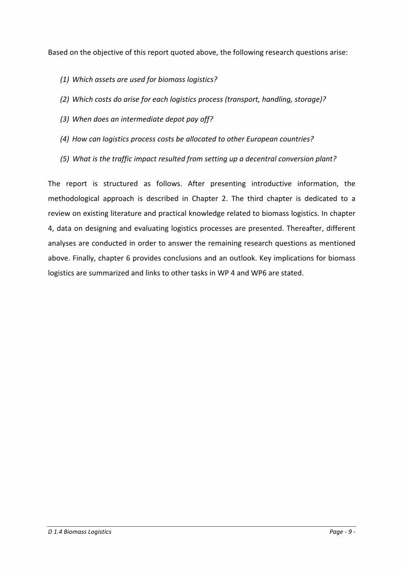
Based on the objective of this report quoted above, the following research questions arise:
(1) Which assets are used for biomass logistics?
(2) Which costs do arise for each logistics process (transport, handling, storage)?
(3) When does an intermediate depot pay off?
(4) How can logistics process costs be allocated to other European countries?
(5) What is the traffic impact resulted from setting up a decentral conversion plant?
The report is structured as follows. After presenting introductive information, the
methodological approach is described in Chapter 2. The third chapter is dedicated to a
review on existing literature and practical knowledge related to biomass logistics. In chapter
4, data on designing and evaluating logistics processes are presented. Thereafter, different
analyses are conducted in order to answer the remaining research questions as mentioned
above. Finally, chapter 6 provides conclusions and an outlook. Key implications for biomass
logistics are summarized and links to other tasks in WP 4 and WP6 are stated.
D 1.4 Biomass Logistics Page - 10 -
2 Methodological Approach
2.1 General Approach
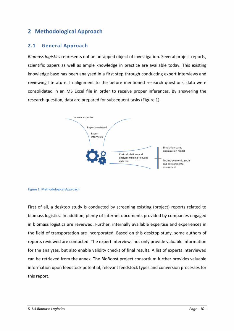
Biomass logistics represents not an untapped object of investigation. Several project reports,
scientific papers as well as ample knowledge in practice are available today. This existing
knowledge base has been analysed in a first step through conducting expert interviews and
reviewing literature. In alignment to the before mentioned research questions, data were
consolidated in an MS Excel file in order to receive proper inferences. By answering the
research question, data are prepared for subsequent tasks (Figure 1).
Figure 1: Methodological Approach
First of all, a desktop study is conducted by screening existing (project) reports related to
biomass logistics. In addition, plenty of internet documents provided by companies engaged
in biomass logistics are reviewed. Further, internally available expertise and experiences in
the field of transportation are incorporated. Based on this desktop study, some authors of
reports reviewed are contacted. The expert interviews not only provide valuable information
for the analyses, but also enable validity checks of final results. A list of experts interviewed
can be retrieved from the annex. The BioBoost project consortium further provides valuable
information upon feedstock potential, relevant feedstock types and conversion processes for
this report.
Internal expertise
Reports reviewed
Expert interviews
Simulation-based optimization model
Techno-economic, social and environmental assessment
Cost calculations and analyses yielding relevant data for:
D 1.4 Biomass Logistics Page - 11 -
2.2 System Boundary
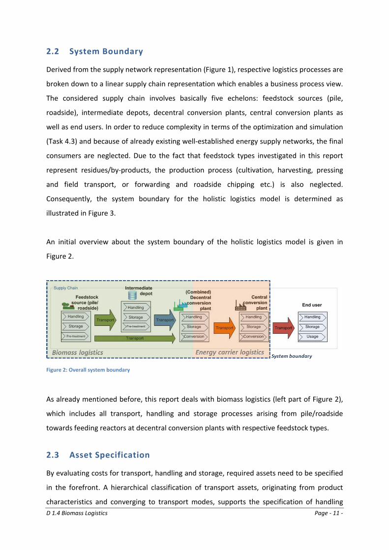
Derived from the supply network representation (Figure 1), respective logistics processes are
broken down to a linear supply chain representation which enables a business process view.
The considered supply chain involves basically five echelons: feedstock sources (pile,
roadside), intermediate depots, decentral conversion plants, central conversion plants as
well as end users. In order to reduce complexity in terms of the optimization and simulation
(Task 4.3) and because of already existing well-established energy supply networks, the final
consumers are neglected. Due to the fact that feedstock types investigated in this report
represent residues/by-products, the production process (cultivation, harvesting, pressing
and field transport, or forwarding and roadside chipping etc.) is also neglected.
Consequently, the system boundary for the holistic logistics model is determined as
illustrated in Figure 3.
An initial overview about the system boundary of the holistic logistics model is given in
Figure 2.
Figure 2: Overall system boundary
As already mentioned before, this report deals with biomass logistics (left part of Figure 2),
which includes all transport, handling and storage processes arising from pile/roadside
towards feeding reactors at decentral conversion plants with respective feedstock types.
2.3 Asset Specification
By evaluating costs for transport, handling and storage, required assets need to be specified
in the forefront. A hierarchical classification of transport assets, originating from product
characteristics and converging to transport modes, supports the specification of handling
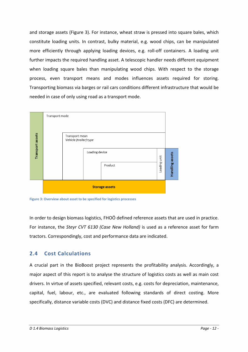
D 1.4 Biomass Logistics Page - 12 -
and storage assets (Figure 3). For instance, wheat straw is pressed into square bales, which
constitute loading units. In contrast, bulky material, e.g. wood chips, can be manipulated
more efficiently through applying loading devices, e.g. roll-off containers. A loading unit
further impacts the required handling asset. A telescopic handler needs different equipment
when loading square bales than manipulating wood chips. With respect to the storage
process, even transport means and modes influences assets required for storing.
Transporting biomass via barges or rail cars conditions different infrastructure that would be
needed in case of only using road as a transport mode.
Figure 3: Overview about asset to be specified for logistics processes
In order to design biomass logistics, FHOÖ defined reference assets that are used in practice.
For instance, the Steyr CVT 6130 (Case New Holland) is used as a reference asset for farm
tractors. Correspondingly, cost and performance data are indicated.
2.4 Cost Calculations
A crucial part in the BioBoost project represents the profitability analysis. Accordingly, a
major aspect of this report is to analyse the structure of logistics costs as well as main cost
drivers. In virtue of assets specified, relevant costs, e.g. costs for depreciation, maintenance,
capital, fuel, labour, etc., are evaluated following standards of direct costing. More
specifically, distance variable costs (DVC) and distance fixed costs (DFC) are determined.
D 1.4 Biomass Logistics Page - 13 -
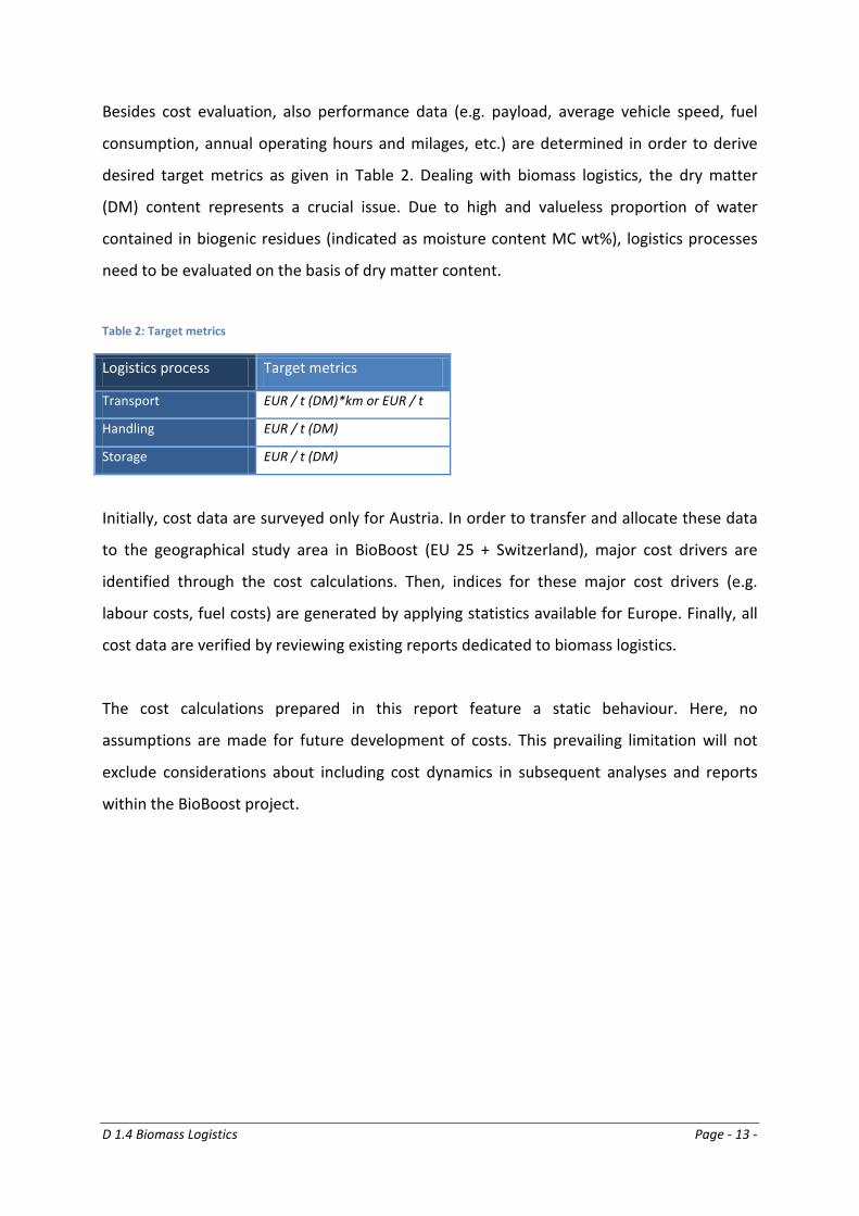
Besides cost evaluation, also performance data (e.g. payload, average vehicle speed, fuel
consumption, annual operating hours and milages, etc.) are determined in order to derive
desired target metrics as given in Table 2. Dealing with biomass logistics, the dry matter
(DM) content represents a crucial issue. Due to high and valueless proportion of water
contained in biogenic residues (indicated as moisture content MC wt%), logistics processes
need to be evaluated on the basis of dry matter content.
Table 2: Target metrics
Logistics process Target metrics
Transport EUR / t (DM)*km or EUR / t
Handling EUR / t (DM)
Storage EUR / t (DM)
Initially, cost data are surveyed only for Austria. In order to transfer and allocate these data
to the geographical study area in BioBoost (EU 25 + Switzerland), major cost drivers are
identified through the cost calculations. Then, indices for these major cost drivers (e.g.
labour costs, fuel costs) are generated by applying statistics available for Europe. Finally, all
cost data are verified by reviewing existing reports dedicated to biomass logistics.
The cost calculations prepared in this report feature a static behaviour. Here, no
assumptions are made for future development of costs. This prevailing limitation will not
exclude considerations about including cost dynamics in subsequent analyses and reports
within the BioBoost project.
D 1.4 Biomass Logistics Page - 14 -
3 Review on Existing Literature and Practical Knowledge
In the course of the previous decades a rethinking in terms of alternative energy sources has
taken place. Renewable energy sources, e.g. biomass, came to the fore and induced plenty
of projects on a national as well as international level. Also the scientific community put
emphasize on this topic. When it comes to how generating energy out of biomass in an
efficient way, logistics play a decisive role. As a matter of fact, plenty of reports dedicated to
biomass logistics have been published recently. The following represents not an exhaustive
but selective abstract of existing literature.
3.1 Literature on Biomass Logistics
The RENEW project (2008), which was run prior to BioBoost, has also dealt with biomass
logistics. More specifically, a concept for biomass provision is evaluated (EUR/GJ) for
agricultural and forestry residues as well as for energy crops. The respective costs are not
only evaluated for a current state (base case), but also for two future scenarios assuming
different levels of feedstock utilization. The overall supply chain is subdivided into two parts:
(1) biomass provision up to the first gathering point and (2) biomass provision from the first
gathering point. Basically, all costs are defined for six regions in Europe.
The BioLog I project (2007) aims at optimizing a supply chain for woody biomass by
minimizing transports in Austria. Based on both an evaluation of disposal feedstock potential
for woody biomass and an existing supply network of biomass conversion plants (BMK3) and
the evaluated feedstock potential, transport costs are minimized through applying a linear
programming (LP) model. In terms of allocating feedstock potential to BMKs, three types of
heuristics are applied: (i) total cost minimum, (ii) market power and (iii) attraction of regions.
By designing an optimal supply network, different types of terminals (agricultural, regional
and industrial) are located through using the mathematical model and assumed logistics
data.
3 BMK = Biomassekraftwerk.
D 1.4 Biomass Logistics Page - 15 -
A further project called Optimierung der regionalen Warenströme (Qualitäten, Transport,
Aufkommen, etc.) über Biomasse-Logistikzentren (2008) puts a strong focus on biomass
logistics centres. More specifically, a location and allocation model that aims at minimizing
transport and preparation costs in Styria (Austria) is set. With respect to the solution
process, a mixed-integer programing (MIP) model and a geographic information system are
used. Among further issues, processes for storage and handling in biomass logistics centres
are designed and evaluated more in detail.
Another, quite recent project Basisinformationen für eine nachhaltige Nutzung von
landwirtschaftlichen Reststoffen zur Bioenergiebereitstellung (2012) deals with straw as an
agricultural residue associated with high potential in Germany for energy generating
purposes. Among others, this project also dedicated its attention towards biomass logistics.
In particular, supply chains are investigated in more detail by determining also logistics
assets. Similar to this report, different options of configuring logistics costs (e.g. type of
vehicle-trailer combination applied) are analysed and evaluated.
In 2005, the Institute for Technology Assessment and Systems Analysis (ITAS) published a
study called Entwicklungen von Szenarien über die Bereitstellung von land- und
forstwirtschaftlicher Biomasse in zwei baden-württembergischen Regionen zur Herstellung
von synthetischen Kraftstoffen (2005). Here, also the feedstock potential for biogenic
residues is evaluated for Germany. Furthermore, supply costs (EUR/Mg DM) for straw, hay,
maize and forest residues are calculated for different transport distance intervals.
The study Leitfaden Bioenergie – Planung, Betrieb und Wirtschaftlichkeit von
Bioenergieanlagen (2005) indicates also valuable information on biomass logistics.
Especially, technical specifications regarding biomass storage, e.g. quality losses of different
feedstock types, storage techniques etc., are mentioned.
D 1.4 Biomass Logistics Page - 16 -
Practical insights into processes within biomass logistics provide the final report from the
project Optimierung der Beschaffungs- und Distributionslogistik bei großen Biogasanlagen
(2007). This project deals with both inbound as well as outbound logistics of biogas plants in
Austria. Especially, technical specification of used assets and work time studies for different
processes are presented in this report.
Further practical insights into converting straw into energy provide the study Straw to
Energy - Status, Technologies and Innovation in Denmark (2011). Especially, types of bales
and assets, e.g. telescopic handler, forklift trucks or gantry cranes, used for handling straw
are specified. The Wood Fuels Handbook (2008) gives insights into main characteristics of log
wood and wood chips. Additionally, this handbook indicated key figures (costs, productivity,
etc.) for assets used along the supply chain.
Regarding the specification of storage assets, the report on Biomass Logistics & Trade
Centers (2010) offers an implementation guide for such BLTCs. More precisely, three steps
are described for a successful project implementation for future BLTC operators. Cost figures
are also incorporated in this report.
With respect to biomass transports, several studies and scientific papers are reviewed. The
Biogas Forum Bayern (2010) published several studies referring to biomass transports. The
BTL Wieselburg (2009) also engages in biomass transportation. Several scientific papers are
available (Handler, 2009 and 2010). Further papers related to biomass transports are
published by Searcy et al. (2007), Singh et al. (2010) as well as Hamelinck et al. (2005).
Besides the projects mentioned above, further scientific work in the field of supply network
planning for bioenergy generation is done. Gold and Seuring (2011) provide a recent
literature review regarding supply chain and logistics issues for biomass-based energy
production. Basically, literature with respect to both (i) operational issues regarding
harvesting and collection, storage, transport and pre-treatment techniques as well as (ii)
strategic issues referring supply system design are reviewed. Moser (2012) engages in
location and capacity planning for Biomass-to-Liquid (BtL) plants in Austria. This thesis
D 1.4 Biomass Logistics Page - 17 -
validates a production network for BtL characterized by a decentral pyrolysis and a central
synthesis as an optimal supply network. Freppaz et al. (2004), Rentizelas et al. (2009),
Velazquez-Marti, Fernandez-Gonzalez (2010), deals with mathematical models as decision
support tools. Perpiñá et al. (2009) apply Geographic Information Systems (GIS) for
optimizing biomass logistics.
Another interesting paper reviewed is given by Lourdes Bravo (2011). Key barriers along a
biofuel supply chain are investigated by applying a comprehensive literature review. This
paper pinpoints variables that may hamper biomass-to-energy development. For instance,
facility location and capacity are variables identified in the context of storage. Storage is a
major cost driver in biomass logistics.
In addition to the reports reviewed, several books have been screened with respect to
(biomass) logistics processes (Gleissner, 2009; Kaltschmitt, 2009; Martin, 2009; Pfohl, 2010;
Weber 2012).
3.2 Practical Knowledge on Biomass Logistics
Besides the reports reviewed, practitioners have been contacted and interviewed in order to
receive and verify data. This is because most of the before mentioned reports make
assumptions in terms of cost data and do not verify the same in a transparent way. The
interviews have been mainly conducted with Austrian organizations that are engaged in
biomass logistics. From governmental agencies and educational and research institutions via
transport, storage as well as biomass power plant operators to motor vehicle/trailer
manufacturers are consulted (a comprehensive list of all experts interviewed can be
retrieved from the annex). The gathered information has a major impact on the validity of
logistics costs, because cost calculations are based upon practical data sets.
D 1.4 Biomass Logistics Page - 18 -
4 Biomass Logistics – Designing and Evaluating Logistics Processes
This chapter aims at examining the design and evaluation of biomass logistics processes. For
this purpose, an MS Excel file, LogisticsProcesses.xlsx, is generated, which incorporates
major computations.
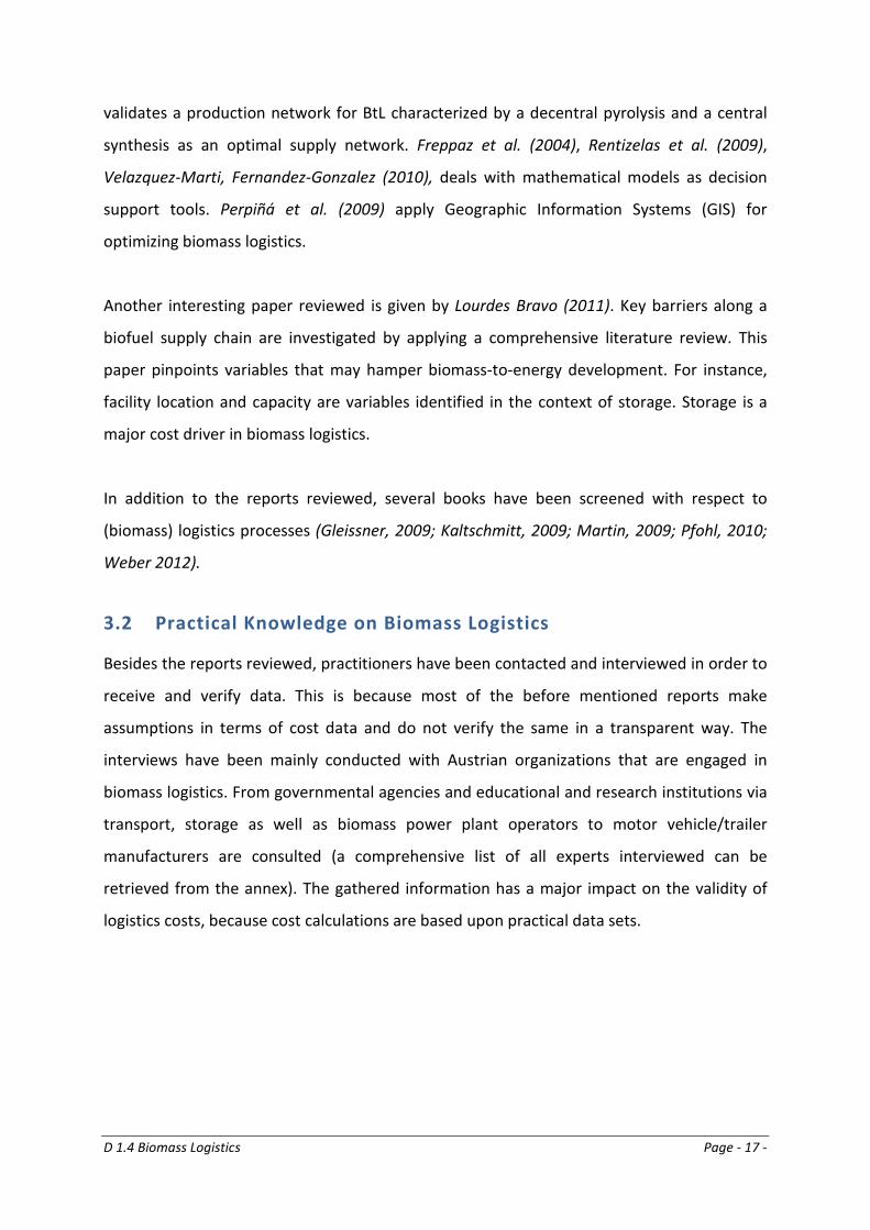
4.1 Biomass Supply Chain in Detail
First of all, the overall supply chain depicted in Figure 4 need to be analysed in more detail.
As already mentioned above, the biomass production process (cultivation, harvest, etc.) is
neglected. The holistic logistics model assumes that respective biogenic residues are
provided at pile or at roadside. The biomass supply chain starts with the storage process at
feedstock source and ends at the decentral conversion plant (DCP) when feeding the
reactors (Figure 4). Correspondingly, the logistics costs are evaluated for this scope.
The respective supply chain exhibits either two or three echelons, that is, biomass residues
are transported directly from the feedstock source to the DCP or biomass residues are first
transported to an intermediate depot (pre-carriage) before further transported to the DCP
(on-carriage). Basically, each echelon features storage and handling processes (loading and
unloading). The transport process occurs between echelons.
D 1.4 Biomass Logistics Page - 19 -
Figure 4: Biomass supply chain in detail
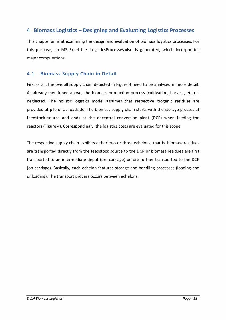
4.2 Specification of Reference Feedstock Types
In the BioBoost project three conversion technologies are examined: (i) fast pyrolysis (FP), (ii)
catalytic pyrolysis (CP) and (iii) hydrothermal carbonization (HTC). As already explained
above, reference feedstock types are defined for each technology.
Table 3: Conversion technology and defined reference feedstock types
Conversion technology Reference feedstock type
Fast pyrolysis (FP) Wheat straw
Catalytic pyrolysis (CP) Wood chips from logging residues
Hydrothermal carbonization (HTC) Organic municipal waste
These types of biogenic residues constitute the main starting point for biomass logistics
analyses. Therein, all processes and required assets are aligned according to the product
specifications.
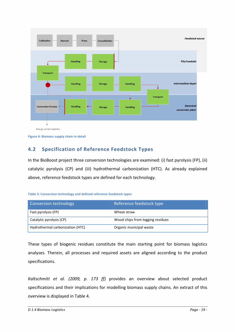
Kaltschmitt et al. (2009, p. 173 ff) provides an overview about selected product
specifications and their implications for modelling biomass supply chains. An extract of this
overview is displayed in Table 4.
D 1.4 Biomass Logistics Page - 20 -
Table 4: Overview about product specification of biomass fuels
A major factor of transporting biomass fuels efficiently is given by the moisture content
(MC). This parameter indicates the amount of water contained in biomass and may vary
considerable. Biomass excluding the moisture content is denoted as dry matter (DM).
Generally, the MC has an essential impact on transport and storage process. Technical
assets, e.g. drying machines, etc. or transport and storage capacities are determined by this
product specification. Storing biomass leads to dry matter losses due to biological
degradation and technical inefficiencies. Therefore, dry matter losses need to be defined for
each feedstock type as well as storage location (DBFZ, 2012, p. 67). The moisture content is
also a crucial figure for conversion technologies in order to work properly. Furthermore, this
parameter may cause an additional pre-treatment process, i.e. drying.
A key figure with respect to product specifications represents the bulk density (BD), because
this parameter influences the efficiency of transport and storage processes substantially
(BOKU, 2007, p. 9). Especially, transporting straw is restricted by available cargo space. In
case of increasing the BD, more square bales can be transported which increase the
utilization of transport means (KRONE, 2012, p. 37). The bulk density represents a
measurement that expresses the weight/volume ratio of materials. In addition to the mass
density, bulk density also considers voids which arise in terms of creating piles of materials
and is determined as kg per m³ (Francescato, V. et al., 2007, p. 8). That is, this ratio provides
information concerning volume and weight of a material, which need to be transported,
handled and stored. With respect to biomass logistics, transports of feedstock types
associated with a low bulk density faces volume restrictions, whereas high density feedstock
types reach payload restrictions (Kaltschmitt et al., 2009, p. 278). In general, the bulk density
of biomass is influenced mainly by (i) moisture content, (ii) type of biomass and (iii) particle
size (Expert interview 4, 2012).
Product specification ofbiomass fuels
Main effects on
Moisture content (MC)
Degradation
Bulk density (BC)
Particle size
Viscosity
Storability, caloric value, dry matter loss, self-heating, transportability
Dry matter loss (technical and biological)
Transport- and storage costs, logistics concept
Pourability, drying properties, dry matter loss
Handling, ability to blend
D 1.4 Biomass Logistics Page - 21 -
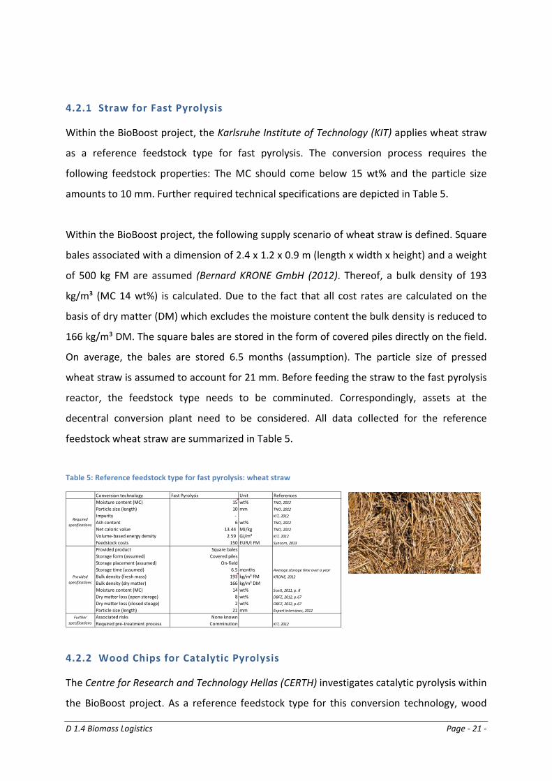
4.2.1 Straw for Fast Pyrolysis
Within the BioBoost project, the Karlsruhe Institute of Technology (KIT) applies wheat straw
as a reference feedstock type for fast pyrolysis. The conversion process requires the
following feedstock properties: The MC should come below 15 wt% and the particle size
amounts to 10 mm. Further required technical specifications are depicted in Table 5.
Within the BioBoost project, the following supply scenario of wheat straw is defined. Square
bales associated with a dimension of 2.4 x 1.2 x 0.9 m (length x width x height) and a weight
of 500 kg FM are assumed (Bernard KRONE GmbH (2012). Thereof, a bulk density of 193
kg/m³ (MC 14 wt%) is calculated. Due to the fact that all cost rates are calculated on the
basis of dry matter (DM) which excludes the moisture content the bulk density is reduced to
166 kg/m³ DM. The square bales are stored in the form of covered piles directly on the field.
On average, the bales are stored 6.5 months (assumption). The particle size of pressed
wheat straw is assumed to account for 21 mm. Before feeding the straw to the fast pyrolysis
reactor, the feedstock type needs to be comminuted. Correspondingly, assets at the
decentral conversion plant need to be considered. All data collected for the reference
feedstock wheat straw are summarized in Table 5.
Table 5: Reference feedstock type for fast pyrolysis: wheat straw
4.2.2 Wood Chips for Catalytic Pyrolysis
The Centre for Research and Technology Hellas (CERTH) investigates catalytic pyrolysis within
the BioBoost project. As a reference feedstock type for this conversion technology, wood
Conversion technology Fast Pyrolysis Unit ReferencesMoisture content (MC) 15 wt% TNO, 2012
Particle size (length) 10 mm TNO, 2012
Impurity - KIT, 2012
Ash content 6 wt% TNO, 2012
Net caloric value 13.44 MJ/kg TNO, 2012
Volume-based energy density 2.59 GJ/m³ KIT, 2012
Feedstock costs 150 EUR/t FM Syncom, 2013
Provided product Square balesStorage form (assumed) Covered pilesStorage placement (assumed) On-fieldStorage time (assumed) 6.5 months Average storage time over a year
Bulk density (fresh mass) 193 kg/m³ FM KRONE, 2012
Bulk density (dry matter) 166 kg/m³ DMMoisture content (MC) 14 wt% Scott, 2011, p. 8
Dry matter loss (open storage) 8 wt% DBFZ, 2012, p.67
Dry matter loss (closed stoage) 2 wt% DBFZ, 2012, p.67
Particle size (length) 21 mm Expert interviews, 2012
Associated risks None knownRequired pre-treatment process Comminution KIT, 2012
Required specifications
Provided specifications
Further specifications
D 1.4 Biomass Logistics Page - 22 -
chips based on logging residues (soft and hardwood) are defined. More precisely, the
following required specifications are indicated. Wood chips to be converted need to exhibit a
moisture content level of smaller than 10 %. Furthermore, the maximum particle size is
given by 5 mm. Besides these parameters, further specifications are made as depicted in
Table 6. Again, there is a divergence between required features for conversion and provided
product characteristics provided at feedstock source.
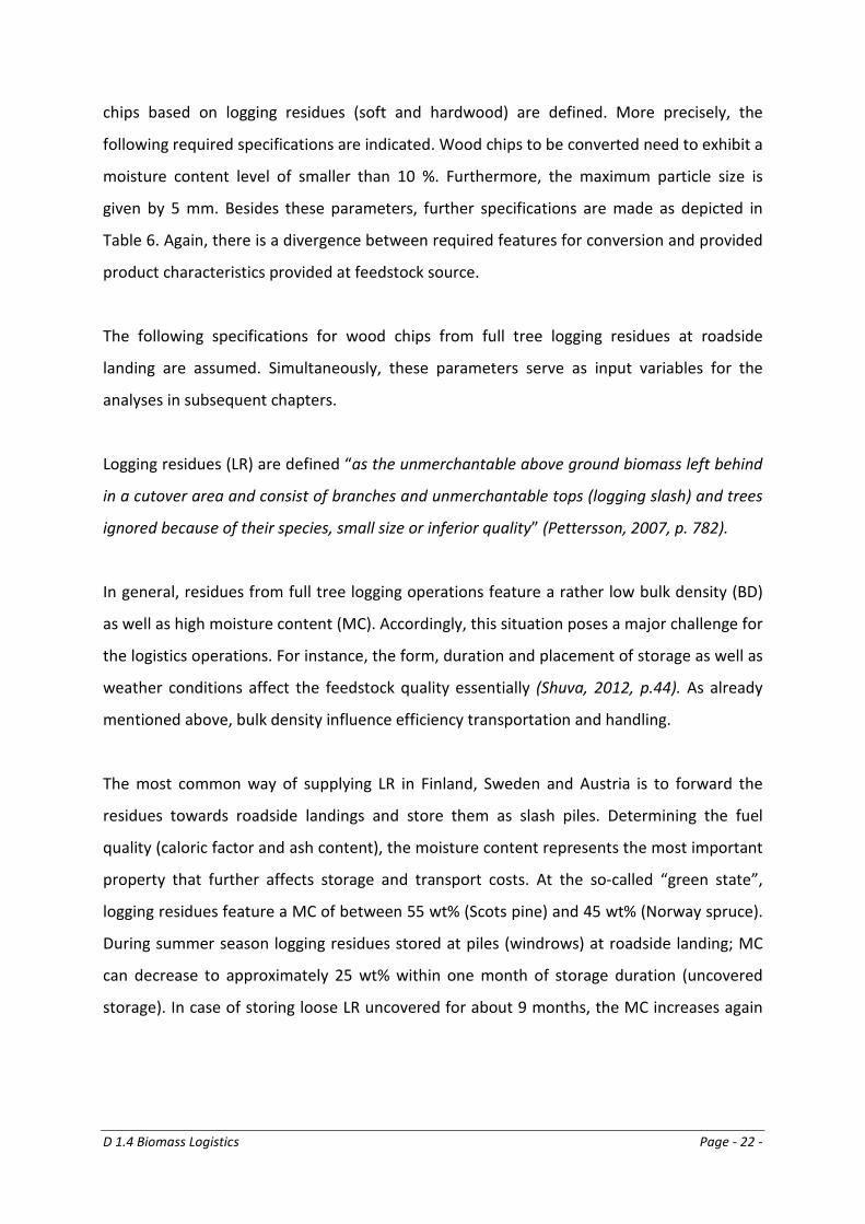
The following specifications for wood chips from full tree logging residues at roadside
landing are assumed. Simultaneously, these parameters serve as input variables for the
analyses in subsequent chapters.
Logging residues (LR) are defined “as the unmerchantable above ground biomass left behind
in a cutover area and consist of branches and unmerchantable tops (logging slash) and trees
ignored because of their species, small size or inferior quality” (Pettersson, 2007, p. 782).
In general, residues from full tree logging operations feature a rather low bulk density (BD)
as well as high moisture content (MC). Accordingly, this situation poses a major challenge for
the logistics operations. For instance, the form, duration and placement of storage as well as
weather conditions affect the feedstock quality essentially (Shuva, 2012, p.44). As already
mentioned above, bulk density influence efficiency transportation and handling.
The most common way of supplying LR in Finland, Sweden and Austria is to forward the
residues towards roadside landings and store them as slash piles. Determining the fuel
quality (caloric factor and ash content), the moisture content represents the most important
property that further affects storage and transport costs. At the so-called “green state”,
logging residues feature a MC of between 55 wt% (Scots pine) and 45 wt% (Norway spruce).
During summer season logging residues stored at piles (windrows) at roadside landing; MC
can decrease to approximately 25 wt% within one month of storage duration (uncovered
storage). In case of storing loose LR uncovered for about 9 months, the MC increases again
D 1.4 Biomass Logistics Page - 23 -
to wt40 % - due to contamination with snow and rain4 (Pettersson, 2007, p. 782f). Therefore,
logging residues are assumed to be comminuted within one month before transportation on
roads.
Further parameters, e.g. ash content and caloric value, are also altered during storage
process, but will not be elaborated here. Instead, the focus is put on the impact of moisture
content on logistics processes. MC influences considerably bulk density and dry matter loss
which represents two important parameters for transport, handling and storage. The former
has already been described above.
“Dry matter losses can be caused either by microbial activity, most commonly fungal attacks
(biological), or spillage of material during handling and storage (technical).” (Pettersson,
2007, p. 785). The dry matter loss for loose logging residues at roadside landing is indicated
by 11 % for the respective storage time. Consequently, this parameter reduces the available
feedstock quantity at the feedstock source.
The underlying supply scenario involves comminution of the before-mentioned logging
residues at roadside landing through applying mobile chippers. This is because of the
motivation of increasing efficiency in road transportation by enhancing bulk density of
logging residues. Here, a bulk density of 276 kg/m³ (MC 30 wt%)5 is assumed. Again as a
matter of the calculation basis, the bulk density is reduced to 193 kg/m³ DM.
Further specifications for wood chips concern associated risks of manipulating this feestock
type as well as required pre-treatment processes. The latter results from the discrepancy of
the above-mentioned required and provided properties. That is, particle sizes (5 mm vs. 30
mm) and moisture content (30 wt% vs. 10 wt%) diverge. Additional comminution and drying
at the decentral conversion plant are necessary and need to be considered in planning the
facilities. The risks affect the logistics processes per se, for instance, security installations due
4 Logging residues can also be stored as compacted residues logs (bundles) produced at roadside landing. This concept implies lower MC rates in case of longer storage times. However, this system is still less well-developed and not broadly applied. 5 A blend of softwood (spruce: 223 kg/m³) and hardwood (beech: 328 kg/m³) is defined as per Francescato, 2008, p.27.
D 1.4 Biomass Logistics Page - 24 -
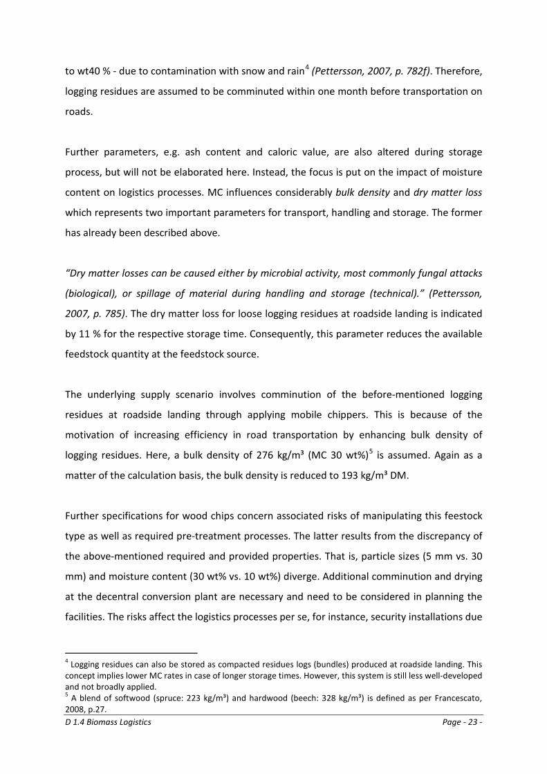
to self-heating of wood chips. This issue is elaborated separately within the BioBoost project.
All specifications are summarized in Table 6.
Table 6: Reference feedstock type for catalytic pyrolysis: wood chips
4.2.3 Organic municipal waste for Hydrothermal Carbonization
A third reference pathway has been defined for hydrothermal carbonization (HTC), which is
examined by AVA-CO2. Here, organic municipal waste is defined as reference feedstock
type. Principally, the moisture content does not play a role for this conversion technology.
Instead, problems are encountered with respect to impurities, e.g. glass, metal, etc.
detected in the waste. This challenge in processing also induces a pre-treatment process
prior to the conversion process: Presorting
Within the BioBoost project it is assumed that organic municipal waste is available at a
certain collection point (e.g. composting plants). Therefore, the waste collection process is
not analysed here. In general, HTC plants are small-dimensioned in relation to FP and CP
plants. Correspondingly, these plants are designed to be located next to major organic waste
collection places. This fact also implies that no logistics processes are examined for this
conversion technology. It is assumed that reactors are fed fully automated through screw-
conveyor. For the sake of completeness, specifications are made also for organic municipal
waste as indicated in Table 7.
Conversion technology Catalytic Pyrolysis Unit ReferencesMoisture content (MC) 8 wt% TNO, 2012
Particle size (length) 5 mm TNO, 2012
Impurity -Ash content 0.54 wt% TNO, 2012
Net caloric value 16.0 MJ/kg Wood fuels handbook, 2008, p. 27
Volume-based energy density 4.41 GJ/m³ TNO, 2012
Feedstock costs 80 EUR/t Syncom, 2013
Provided product 1 Logging residues (loose)Moisture content (MC) 55 wt% Shuva, 2012. "green state"
Storage form (assumed) Covered windrows (slash piles) Specified within storage process
Storage placement (assumed) Roadside landingStorage time (assumed) 1 month Pettersson, 2007, p.789
Moisture content (MC) reduced 28 wt% Pettersson, 2007, p.783
Dry matter loss at roadside landing 0.9 wt% Pettersson, 2007, p.791
Provided product 2 Wood chipsBulk density (fresh mass) 276 kg/m³ FM Annex (Average of Beech and Spruce)
Bulk density (dry matter) 193 kg/m³ DMMoisture content (MC) 30 wt% Francescato, 2008, p. 11
Dry matter loss (closed storage) 3 wt% (p.a.) Francescato, 2008, p.46
Particle size (length) 30 mm ÖNORM M 7133 (G30)
Associated risks Self-heating > 100°C Francescato, 2008, p.44
Required pre-treatment process Comminution & drying
Required specifications
Provided specifications
Furhter specifications
D 1.4 Biomass Logistics Page - 25 -
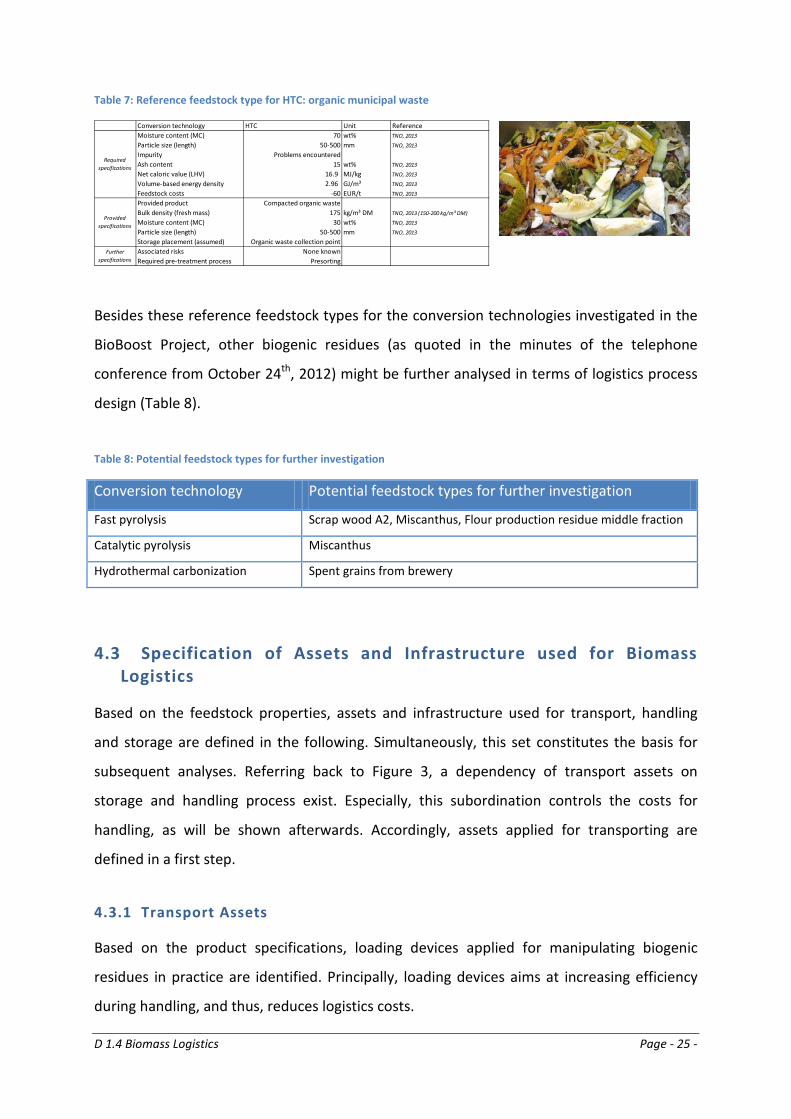
Table 7: Reference feedstock type for HTC: organic municipal waste
Besides these reference feedstock types for the conversion technologies investigated in the
BioBoost Project, other biogenic residues (as quoted in the minutes of the telephone
conference from October 24th, 2012) might be further analysed in terms of logistics process
design (Table 8).
Table 8: Potential feedstock types for further investigation
Conversion technology Potential feedstock types for further investigation
Fast pyrolysis Scrap wood A2, Miscanthus, Flour production residue middle fraction
Catalytic pyrolysis Miscanthus
Hydrothermal carbonization Spent grains from brewery
4.3 Specification of Assets and Infrastructure used for Biomass Logistics
Based on the feedstock properties, assets and infrastructure used for transport, handling
and storage are defined in the following. Simultaneously, this set constitutes the basis for
subsequent analyses. Referring back to Figure 3, a dependency of transport assets on
storage and handling process exist. Especially, this subordination controls the costs for
handling, as will be shown afterwards. Accordingly, assets applied for transporting are
defined in a first step.
4.3.1 Transport Assets
Based on the product specifications, loading devices applied for manipulating biogenic
residues in practice are identified. Principally, loading devices aims at increasing efficiency
during handling, and thus, reduces logistics costs.
Conversion technology HTC Unit ReferenceMoisture content (MC) 70 wt% TNO, 2013
Particle size (length) 50-500 mm TNO, 2013
Impurity Problems encounteredAsh content 15 wt% TNO, 2013
Net caloric value (LHV) 16.9 MJ/kg TNO, 2013
Volume-based energy density 2.96 GJ/m³ TNO, 2013
Feedstock costs -60 EUR/t TNO, 2013
Provided product Compacted organic wasteBulk density (fresh mass) 175 kg/m³ DM TNO, 2013 (150-200 kg/m³ DM)
Moisture content (MC) 30 wt% TNO, 2013
Particle size (length) 50-500 mm TNO, 2013
Storage placement (assumed) Organic waste collection pointAssociated risks None knownRequired pre-treatment process Presorting
Further specifications
Provided specifications
Required specifications
D 1.4 Biomass Logistics Page - 26 -
The combination of the product and loading device is defined as loading unit. For instance, a
40 m³ roll-off container loaded with wood chips represents a loading unit. A loading device is
mainly characterized by its dimensions (metre), payload (ton) and cargo space (cubic metre).
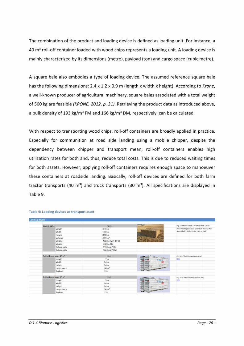
A square bale also embodies a type of loading device. The assumed reference square bale
has the following dimensions: 2.4 x 1.2 x 0.9 m (length x width x height). According to Krone,
a well-known producer of agricultural machinery, square bales associated with a total weight
of 500 kg are feasible (KRONE, 2012, p. 31). Retrieving the product data as introduced above,
a bulk density of 193 kg/m³ FM and 166 kg/m³ DM, respectively, can be calculated.
With respect to transporting wood chips, roll-off containers are broadly applied in practice.
Especially for communition at road side landing using a mobile chipper, despite the
dependency between chipper and transport mean, roll-off containers enables high
utilization rates for both and, thus, reduce total costs. This is due to reduced waiting times
for both assets. However, applying roll-off containers requires enough space to manoeuver
these containers at roadside landing. Basically, roll-off devices are defined for both farm
tractor transports (40 m³) and truck transports (30 m³). All specifications are displayed in
Table 9.
Table 9: Loading devices as transport asset
D 1.4 Biomass Logistics Page - 27 -
These loading devices are used in combination with transport means. Generally, transport
means can be categorized according the transport modes road, rail, waterway, air and
pipeline. Within the BioBoost project, only road and rail transportation are examined.
Subordinately, transport means are compose of different vehicle and trailer types. For
biomass logistics, only road transport and the following vehicle-trailer combinations are
analysed for the selected feedstock types (Table 10).
D 1.4 Biomass Logistics Page - 28 -
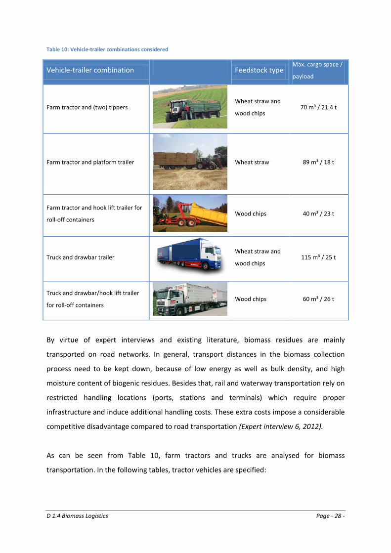
Table 10: Vehicle-trailer combinations considered
Vehicle-trailer combination Feedstock type Max. cargo space /
payload
Farm tractor and (two) tippers
Wheat straw and
wood chips 70 m³ / 21.4 t
Farm tractor and platform trailer
Wheat straw 89 m³ / 18 t
Farm tractor and hook lift trailer for
roll-off containers
Wood chips 40 m³ / 23 t
Truck and drawbar trailer
Wheat straw and
wood chips 115 m³ / 25 t
Truck and drawbar/hook lift trailer
for roll-off containers
Wood chips 60 m³ / 26 t
By virtue of expert interviews and existing literature, biomass residues are mainly
transported on road networks. In general, transport distances in the biomass collection
process need to be kept down, because of low energy as well as bulk density, and high
moisture content of biogenic residues. Besides that, rail and waterway transportation rely on
restricted handling locations (ports, stations and terminals) which require proper
infrastructure and induce additional handling costs. These extra costs impose a considerable
competitive disadvantage compared to road transportation (Expert interview 6, 2012).
As can be seen from Table 10, farm tractors and trucks are analysed for biomass
transportation. In the following tables, tractor vehicles are specified:
D 1.4 Biomass Logistics Page - 29 -
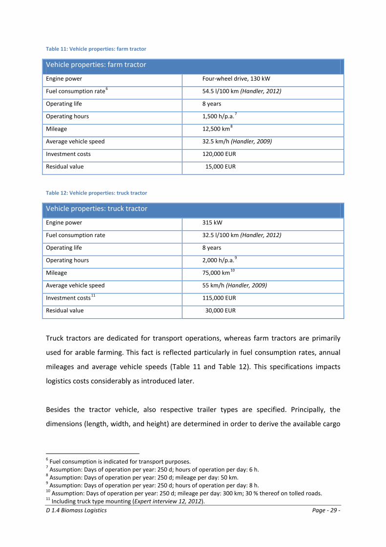
Table 11: Vehicle properties: farm tractor
Vehicle properties: farm tractor
Engine power Four-wheel drive, 130 kW
Fuel consumption rate6 54.5 l/100 km (Handler, 2012)
Operating life 8 years
Operating hours 1,500 h/p.a.7
Mileage 12,500 km8
Average vehicle speed 32.5 km/h (Handler, 2009)
Investment costs 120,000 EUR
Residual value 15,000 EUR
Table 12: Vehicle properties: truck tractor
Vehicle properties: truck tractor
Engine power 315 kW
Fuel consumption rate 32.5 l/100 km (Handler, 2012)
Operating life 8 years
Operating hours 2,000 h/p.a.9
Mileage 75,000 km10
Average vehicle speed 55 km/h (Handler, 2009)
Investment costs11 115,000 EUR
Residual value 30,000 EUR
Truck tractors are dedicated for transport operations, whereas farm tractors are primarily
used for arable farming. This fact is reflected particularly in fuel consumption rates, annual
mileages and average vehicle speeds (Table 11 and Table 12). This specifications impacts
logistics costs considerably as introduced later.
Besides the tractor vehicle, also respective trailer types are specified. Principally, the
dimensions (length, width, and height) are determined in order to derive the available cargo
6 Fuel consumption is indicated for transport purposes. 7 Assumption: Days of operation per year: 250 d; hours of operation per day: 6 h. 8 Assumption: Days of operation per year: 250 d; mileage per day: 50 km. 9 Assumption: Days of operation per year: 250 d; hours of operation per day: 8 h. 10 Assumption: Days of operation per year: 250 d; mileage per day: 300 km; 30 % thereof on tolled roads. 11 Including truck type mounting (Expert interview 12, 2012).
D 1.4 Biomass Logistics Page - 30 -
space and the maximum payload are indicated. In doing so, reference trailer types applied in
practice are characterized as follows (Table 13).
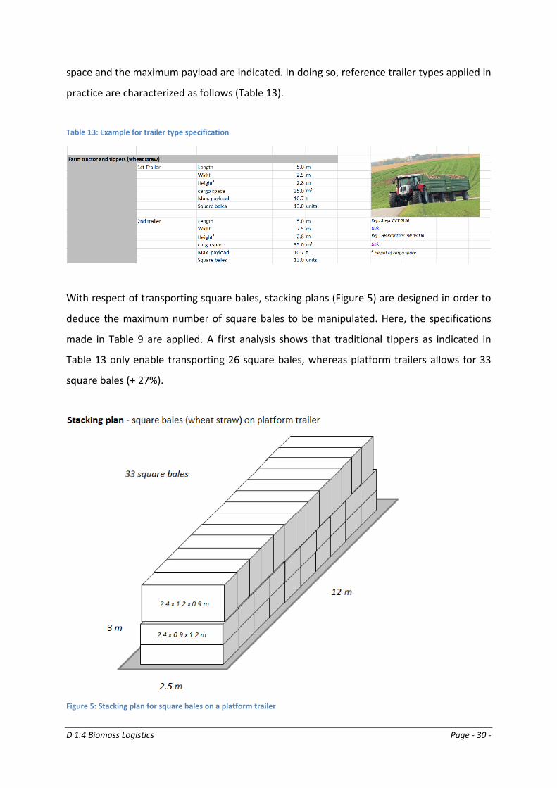
Table 13: Example for trailer type specification
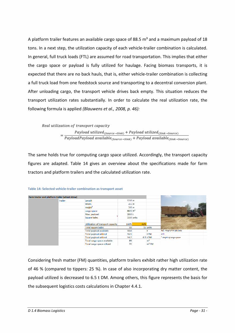
With respect of transporting square bales, stacking plans (Figure 5) are designed in order to
deduce the maximum number of square bales to be manipulated. Here, the specifications
made in Table 9 are applied. A first analysis shows that traditional tippers as indicated in
Table 13 only enable transporting 26 square bales, whereas platform trailers allows for 33
square bales (+ 27%).
Figure 5: Stacking plan for square bales on a platform trailer
D 1.4 Biomass Logistics Page - 31 -
A platform trailer features an available cargo space of 88.5 m³ and a maximum payload of 18
tons. In a next step, the utilization capacity of each vehicle-trailer combination is calculated.
In general, full truck loads (FTL) are assumed for road transportation. This implies that either
the cargo space or payload is fully utilized for haulage. Facing biomass transports, it is
expected that there are no back hauls, that is, either vehicle-trailer combination is collecting
a full truck load from one feedstock source and transporting to a decentral conversion plant.
After unloading cargo, the transport vehicle drives back empty. This situation reduces the
transport utilization rates substantially. In order to calculate the real utilization rate, the
following formula is applied (Blauwens et al., 2008, p. 46):
𝑅𝑒𝑎𝑙 𝑢𝑡𝑖𝑙𝑖𝑧𝑎𝑡𝑖𝑜𝑛 𝑜𝑓 𝑡𝑟𝑎𝑛𝑠𝑝𝑜𝑟𝑡 𝑐𝑎𝑝𝑎𝑐𝑖𝑡𝑦
=𝑃𝑎𝑦𝑙𝑜𝑎𝑑 𝑢𝑡𝑖𝑙𝑖𝑧𝑒𝑑(𝑆𝑜𝑢𝑟𝑐𝑒→𝑆𝑖𝑛𝑘) + 𝑃𝑎𝑦𝑙𝑜𝑎𝑑 𝑢𝑡𝑖𝑙𝑖𝑧𝑒𝑑(𝑆𝑖𝑛𝑘→𝑆𝑜𝑢𝑟𝑐𝑒)
𝑃𝑎𝑦𝑙𝑜𝑎𝑑𝑃𝑎𝑦𝑙𝑜𝑎𝑑 𝑎𝑣𝑎𝑖𝑙𝑎𝑏𝑙𝑒(𝑆𝑜𝑢𝑟𝑐𝑒→𝑆𝑖𝑛𝑘) + 𝑃𝑎𝑦𝑙𝑜𝑎𝑑 𝑎𝑣𝑎𝑖𝑙𝑎𝑏𝑙𝑒(𝑆𝑖𝑛𝑘→𝑆𝑜𝑢𝑟𝑐𝑒)
The same holds true for computing cargo space utilized. Accordingly, the transport capacity
figures are adapted. Table 14 gives an overview about the specifications made for farm
tractors and platform trailers and the calculated utilization rate.
Table 14: Selected vehicle-trailer combination as transport asset
Considering fresh matter (FM) quantities, platform trailers exhibit rather high utilization rate
of 46 % (compared to tippers: 25 %). In case of also incorporating dry matter content, the
payload utilized is decreased to 6.5 t DM. Among others, this figure represents the basis for
the subsequent logistics costs calculations in Chapter 4.4.1.
D 1.4 Biomass Logistics Page - 32 -
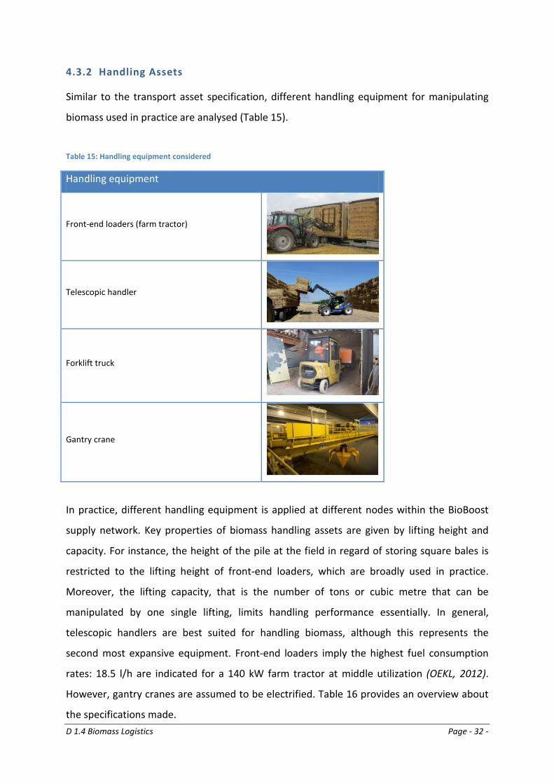
4.3.2 Handling Assets
Similar to the transport asset specification, different handling equipment for manipulating
biomass used in practice are analysed (Table 15).
Table 15: Handling equipment considered
Handling equipment
Front-end loaders (farm tractor)
Telescopic handler
Forklift truck
Gantry crane
In practice, different handling equipment is applied at different nodes within the BioBoost
supply network. Key properties of biomass handling assets are given by lifting height and
capacity. For instance, the height of the pile at the field in regard of storing square bales is
restricted to the lifting height of front-end loaders, which are broadly used in practice.
Moreover, the lifting capacity, that is the number of tons or cubic metre that can be
manipulated by one single lifting, limits handling performance essentially. In general,
telescopic handlers are best suited for handling biomass, although this represents the
second most expansive equipment. Front-end loaders imply the highest fuel consumption
rates: 18.5 l/h are indicated for a 140 kW farm tractor at middle utilization (OEKL, 2012).
However, gantry cranes are assumed to be electrified. Table 16 provides an overview about
the specifications made.
D 1.4 Biomass Logistics Page - 33 -
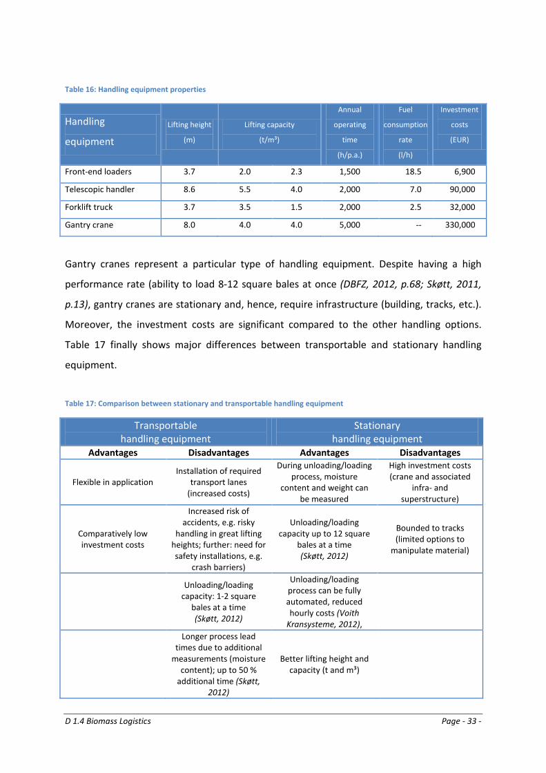
Table 16: Handling equipment properties
Handling
equipment
Lifting height
(m)
Lifting capacity
(t/m³)
Annual
operating
time
(h/p.a.)
Fuel
consumption
rate
(l/h)
Investment
costs
(EUR)
Front-end loaders 3.7 2.0 2.3 1,500 18.5 6,900
Telescopic handler 8.6 5.5 4.0 2,000 7.0 90,000
Forklift truck 3.7 3.5 1.5 2,000 2.5 32,000
Gantry crane 8.0 4.0 4.0 5,000 -- 330,000
Gantry cranes represent a particular type of handling equipment. Despite having a high
performance rate (ability to load 8-12 square bales at once (DBFZ, 2012, p.68; Skøtt, 2011,
p.13), gantry cranes are stationary and, hence, require infrastructure (building, tracks, etc.).
Moreover, the investment costs are significant compared to the other handling options.
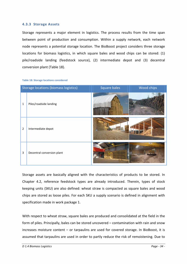
Table 17 finally shows major differences between transportable and stationary handling
equipment.
Table 17: Comparison between stationary and transportable handling equipment
Transportable handling equipment
Stationary handling equipment
Advantages Disadvantages Advantages Disadvantages
Flexible in application Installation of required
transport lanes (increased costs)
During unloading/loading process, moisture
content and weight can be measured
High investment costs (crane and associated
infra- and superstructure)
Comparatively low investment costs
Increased risk of accidents, e.g. risky
handling in great lifting heights; further: need for safety installations, e.g.
crash barriers)
Unloading/loading capacity up to 12 square
bales at a time (Skøtt, 2012)
Bounded to tracks (limited options to
manipulate material)
Unloading/loading capacity: 1-2 square
bales at a time (Skøtt, 2012)
Unloading/loading process can be fully automated, reduced hourly costs (Voith
Kransysteme, 2012),
Longer process lead times due to additional
measurements (moisture content); up to 50 %
additional time (Skøtt, 2012)
Better lifting height and capacity (t and m³)
D 1.4 Biomass Logistics Page - 34 -
4.3.3 Storage Assets
Storage represents a major element in logistics. The process results from the time span
between point of production and consumption. Within a supply network, each network
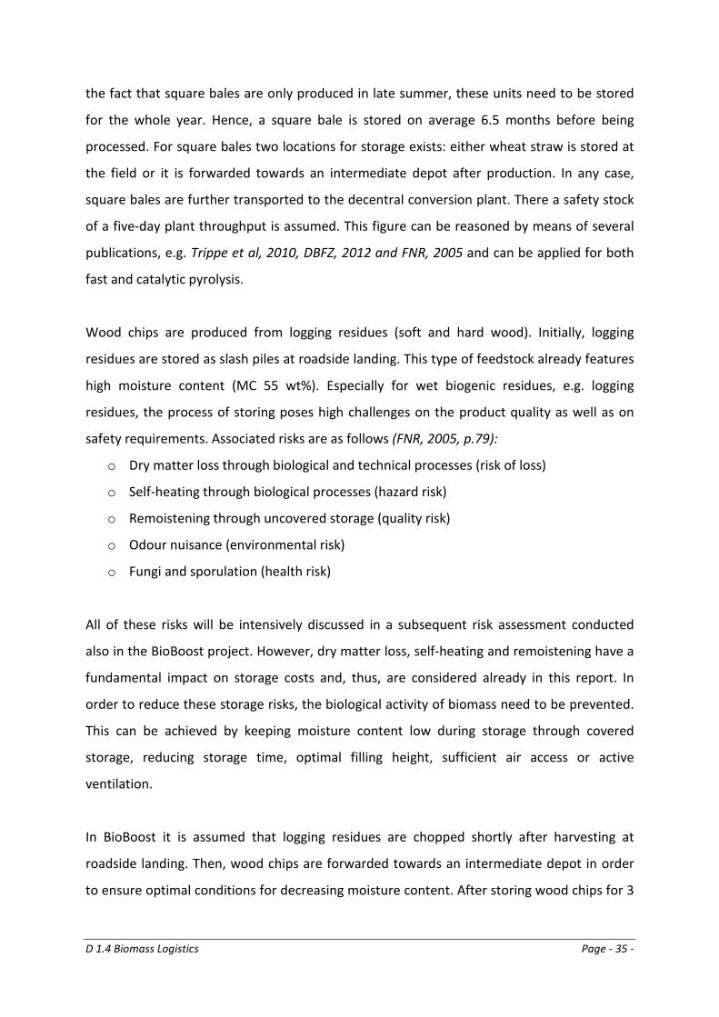
node represents a potential storage location. The BioBoost project considers three storage
locations for biomass logistics, in which square bales and wood chips can be stored: (1)
pile/roadside landing (feedstock source), (2) intermediate depot and (3) decentral
conversion plant (Table 18).
Table 18: Storage locations considered
Storage locations (biomass logistics) Square bales Wood chips
1 Piles/roadside landing
2 Intermediate depot
3 Decentral conversion plant
Storage assets are basically aligned with the characteristics of products to be stored. In
Chapter 4.2, reference feedstock types are already introduced. Therein, types of stock
keeping units (SKU) are also defined: wheat straw is compacted as square bales and wood
chips are stored as loose piles. For each SKU a supply scenario is defined in alignment with
specification made in work package 1.
With respect to wheat straw, square bales are produced and consolidated at the field in the
form of piles. Principally, bales can be stored uncovered – contamination with rain and snow
increases moisture content – or tarpaulins are used for covered storage. In BioBoost, it is
assumed that tarpaulins are used in order to partly reduce the risk of remoistening. Due to
D 1.4 Biomass Logistics Page - 35 -
the fact that square bales are only produced in late summer, these units need to be stored
for the whole year. Hence, a square bale is stored on average 6.5 months before being
processed. For square bales two locations for storage exists: either wheat straw is stored at
the field or it is forwarded towards an intermediate depot after production. In any case,
square bales are further transported to the decentral conversion plant. There a safety stock
of a five-day plant throughput is assumed. This figure can be reasoned by means of several
publications, e.g. Trippe et al, 2010, DBFZ, 2012 and FNR, 2005 and can be applied for both
fast and catalytic pyrolysis.
Wood chips are produced from logging residues (soft and hard wood). Initially, logging
residues are stored as slash piles at roadside landing. This type of feedstock already features
high moisture content (MC 55 wt%). Especially for wet biogenic residues, e.g. logging
residues, the process of storing poses high challenges on the product quality as well as on
safety requirements. Associated risks are as follows (FNR, 2005, p.79):
o Dry matter loss through biological and technical processes (risk of loss)
o Self-heating through biological processes (hazard risk)
o Remoistening through uncovered storage (quality risk)
o Odour nuisance (environmental risk)
o Fungi and sporulation (health risk)
All of these risks will be intensively discussed in a subsequent risk assessment conducted
also in the BioBoost project. However, dry matter loss, self-heating and remoistening have a
fundamental impact on storage costs and, thus, are considered already in this report. In
order to reduce these storage risks, the biological activity of biomass need to be prevented.
This can be achieved by keeping moisture content low during storage through covered
storage, reducing storage time, optimal filling height, sufficient air access or active
ventilation.
In BioBoost it is assumed that logging residues are chopped shortly after harvesting at
roadside landing. Then, wood chips are forwarded towards an intermediate depot in order
to ensure optimal conditions for decreasing moisture content. After storing wood chips for 3
D 1.4 Biomass Logistics Page - 36 -
months at the intermediate depot, it is transported to the decentral conversion plant. There,
a safety stock of a five-day plant throughput is hold, too.
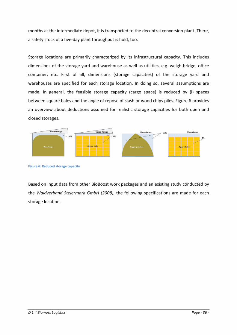
Storage locations are primarily characterized by its infrastructural capacity. This includes
dimensions of the storage yard and warehouse as well as utilities, e.g. weigh-bridge, office
container, etc. First of all, dimensions (storage capacities) of the storage yard and
warehouses are specified for each storage location. In doing so, several assumptions are
made. In general, the feasible storage capacity (cargo space) is reduced by (i) spaces
between square bales and the angle of repose of slash or wood chips piles. Figure 6 provides
an overview about deductions assumed for realistic storage capacities for both open and
closed storages.
Figure 6: Reduced storage capacity
Based on input data from other BioBoost work packages and an existing study conducted by
the Waldverband Steiermark GmbH (2008), the following specifications are made for each
storage location.
D 1.4 Biomass Logistics Page - 37 -
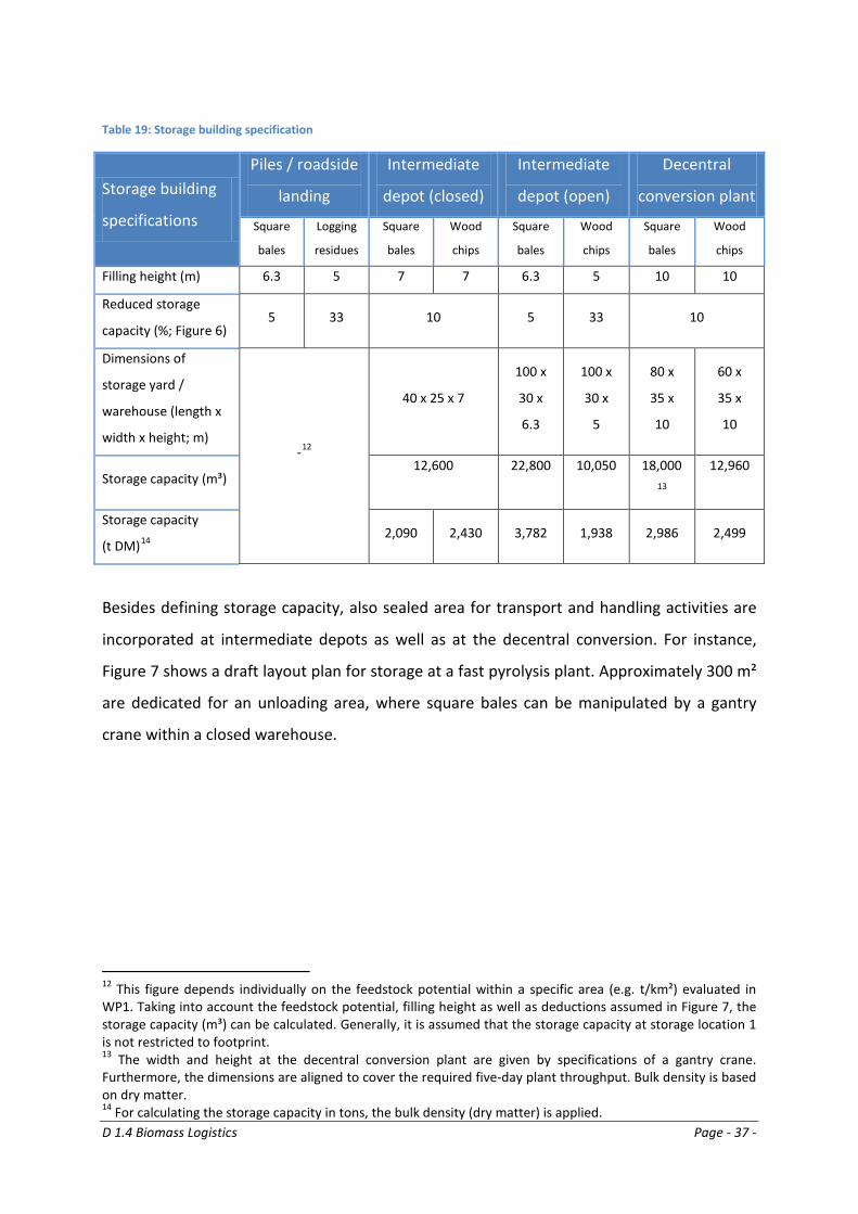
Table 19: Storage building specification
Storage building
specifications
Piles / roadside
landing
Intermediate
depot (closed)
Intermediate
depot (open)
Decentral
conversion plant
Square
bales
Logging
residues
Square
bales
Wood
chips
Square
bales
Wood
chips
Square
bales
Wood
chips
Filling height (m) 6.3 5 7 7 6.3 5 10 10
Reduced storage
capacity (%; Figure 6) 5 33 10 5 33 10
Dimensions of
storage yard /
warehouse (length x
width x height; m) -12
40 x 25 x 7
100 x
30 x
6.3
100 x
30 x
5
80 x
35 x
10
60 x
35 x
10
Storage capacity (m³) 12,600 22,800 10,050 18,000
13
12,960
Storage capacity
(t DM)14 2,090 2,430 3,782 1,938 2,986 2,499
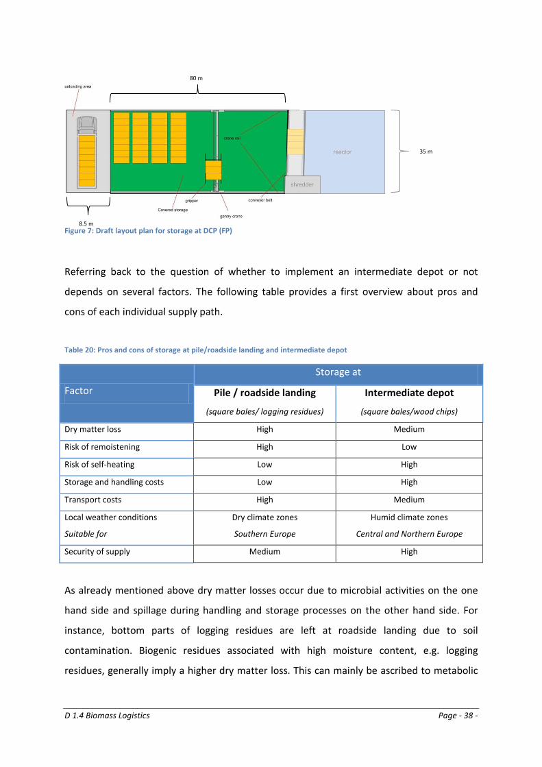
Besides defining storage capacity, also sealed area for transport and handling activities are
incorporated at intermediate depots as well as at the decentral conversion. For instance,
Figure 7 shows a draft layout plan for storage at a fast pyrolysis plant. Approximately 300 m²
are dedicated for an unloading area, where square bales can be manipulated by a gantry
crane within a closed warehouse.
12 This figure depends individually on the feedstock potential within a specific area (e.g. t/km²) evaluated in WP1. Taking into account the feedstock potential, filling height as well as deductions assumed in Figure 7, the storage capacity (m³) can be calculated. Generally, it is assumed that the storage capacity at storage location 1 is not restricted to footprint. 13 The width and height at the decentral conversion plant are given by specifications of a gantry crane. Furthermore, the dimensions are aligned to cover the required five-day plant throughput. Bulk density is based on dry matter. 14 For calculating the storage capacity in tons, the bulk density (dry matter) is applied.
D 1.4 Biomass Logistics Page - 38 -
Figure 7: Draft layout plan for storage at DCP (FP)
Referring back to the question of whether to implement an intermediate depot or not
depends on several factors. The following table provides a first overview about pros and
cons of each individual supply path.
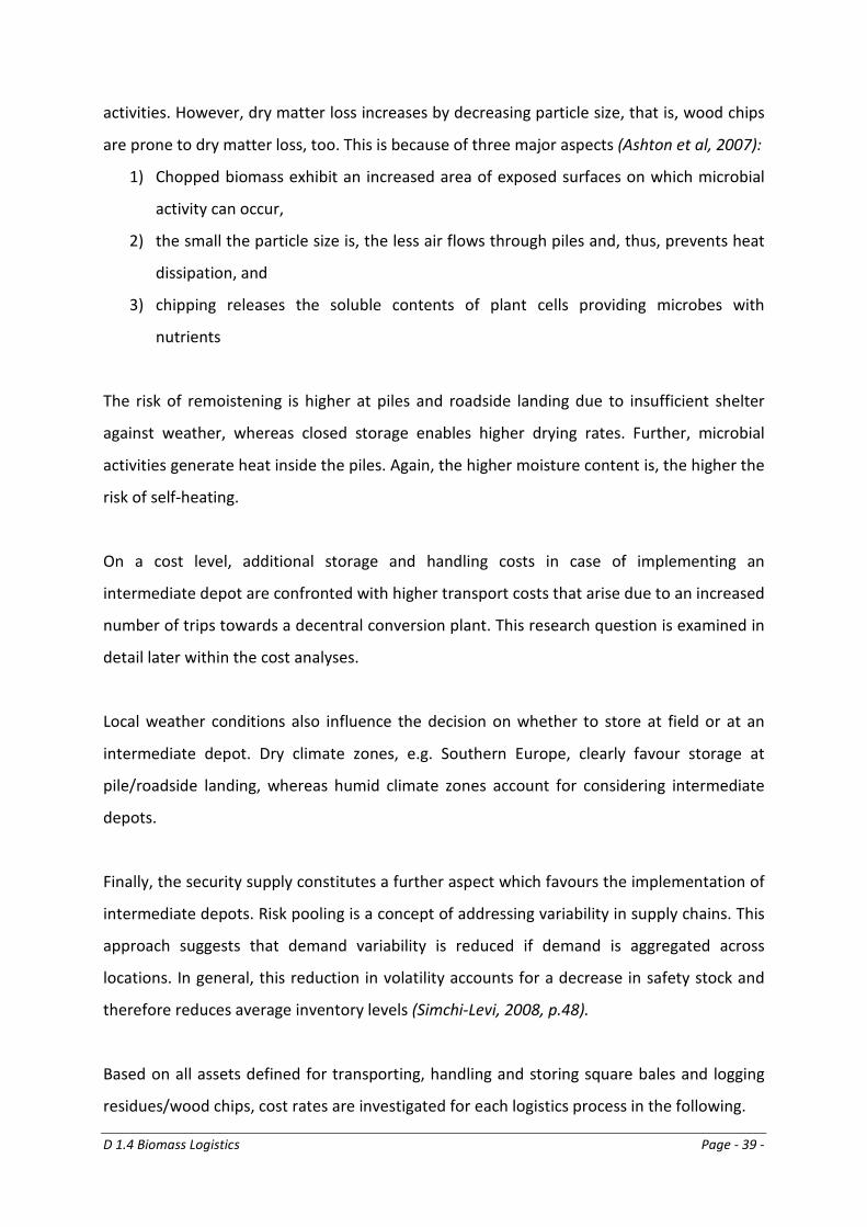
Table 20: Pros and cons of storage at pile/roadside landing and intermediate depot
Factor
Storage at
Pile / roadside landing
(square bales/ logging residues)
Intermediate depot
(square bales/wood chips)
Dry matter loss High Medium
Risk of remoistening High Low
Risk of self-heating Low High
Storage and handling costs Low High
Transport costs High Medium
Local weather conditions
Suitable for
Dry climate zones
Southern Europe
Humid climate zones
Central and Northern Europe
Security of supply Medium High
As already mentioned above dry matter losses occur due to microbial activities on the one
hand side and spillage during handling and storage processes on the other hand side. For
instance, bottom parts of logging residues are left at roadside landing due to soil
contamination. Biogenic residues associated with high moisture content, e.g. logging
residues, generally imply a higher dry matter loss. This can mainly be ascribed to metabolic
80 m
35 m
8.5 m
D 1.4 Biomass Logistics Page - 39 -
activities. However, dry matter loss increases by decreasing particle size, that is, wood chips
are prone to dry matter loss, too. This is because of three major aspects (Ashton et al, 2007):
1) Chopped biomass exhibit an increased area of exposed surfaces on which microbial
activity can occur,
2) the small the particle size is, the less air flows through piles and, thus, prevents heat
dissipation, and
3) chipping releases the soluble contents of plant cells providing microbes with
nutrients
The risk of remoistening is higher at piles and roadside landing due to insufficient shelter
against weather, whereas closed storage enables higher drying rates. Further, microbial
activities generate heat inside the piles. Again, the higher moisture content is, the higher the
risk of self-heating.
On a cost level, additional storage and handling costs in case of implementing an
intermediate depot are confronted with higher transport costs that arise due to an increased
number of trips towards a decentral conversion plant. This research question is examined in
detail later within the cost analyses.
Local weather conditions also influence the decision on whether to store at field or at an
intermediate depot. Dry climate zones, e.g. Southern Europe, clearly favour storage at
pile/roadside landing, whereas humid climate zones account for considering intermediate
depots.
Finally, the security supply constitutes a further aspect which favours the implementation of
intermediate depots. Risk pooling is a concept of addressing variability in supply chains. This
approach suggests that demand variability is reduced if demand is aggregated across
locations. In general, this reduction in volatility accounts for a decrease in safety stock and
therefore reduces average inventory levels (Simchi-Levi, 2008, p.48).
Based on all assets defined for transporting, handling and storing square bales and logging
residues/wood chips, cost rates are investigated for each logistics process in the following.
D 1.4 Biomass Logistics Page - 40 -
4.4 Cost Calculations for Biomass Logistics Processes
As a crucial input for the holistic logistics model, costs for transport, handling and storage
are calculate. The target metrics are already indicated in Table 2. The following assumptions
hold:
o Direct costing (including variable and fixed costs) is applied
o All costs are given on a net basis (excluding value added taxes)
o Annual interest rate is given by 4 % p.a.
o Fuel costs (diesel) amounts to 1.27 EUR/l
o Maintenance rate are as per VDI 2067
o Labour costs (gross wage) are given by 22.53 EUR/h or 35,820 EUR/p.a.
(details see Annex)
o No subsidies are considered
As already indicated in Table 2 the target metrics are EUR/t (DM)*km (transport process)
and EUR/t (DM) (handling and storage process). These cost rates are calculated on a dry
matter basis, because no one would pay for water.
4.4.1 Transport Costs
Based on the specifications made above concerning transport assets, all vehicle-trailer
combinations are evaluated according to their direct costs. Specifically, variable, i.e. distance
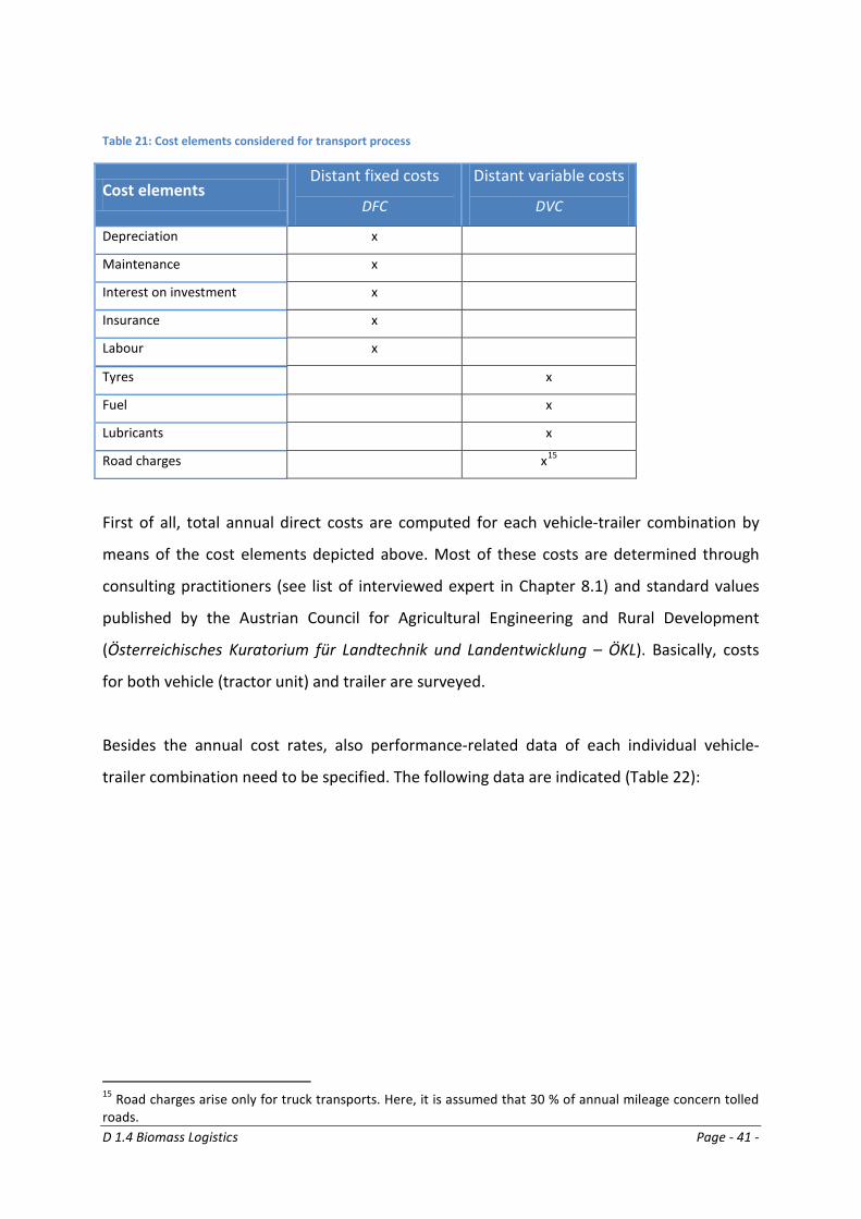
variable costs (DVC), as well as fixed costs, i.e. distance fixed costs (DFC) are identified. Table
21 shows cost elements considered for transport costs evaluation. Usually, costs for
transporting biomass are defined as EUR/t DM, provided that a fixed catchment area is given
(DBFZ, 2012, p.75; Leible, 2005, p.32). As already mentioned, dry matter basis represents a
meaningful basis for biomass logistics cost calculation. Because of applying a real routing
network for Europe within the BioBoost project, transport costs need to be aligned with the
holistic logistics model. Therefore, transport costs are calculated in the form of EUR/t
(DM)*km.
D 1.4 Biomass Logistics Page - 41 -
Table 21: Cost elements considered for transport process
Cost elements Distant fixed costs
DFC
Distant variable costs
DVC
Depreciation x
Maintenance x
Interest on investment x
Insurance x
Labour x
Tyres x
Fuel x
Lubricants x
Road charges x15
First of all, total annual direct costs are computed for each vehicle-trailer combination by
means of the cost elements depicted above. Most of these costs are determined through
consulting practitioners (see list of interviewed expert in Chapter 8.1) and standard values
published by the Austrian Council for Agricultural Engineering and Rural Development
(Österreichisches Kuratorium für Landtechnik und Landentwicklung – ÖKL). Basically, costs
for both vehicle (tractor unit) and trailer are surveyed.
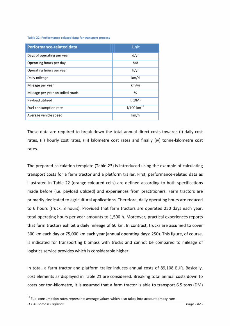
Besides the annual cost rates, also performance-related data of each individual vehicle-
trailer combination need to be specified. The following data are indicated (Table 22):
15 Road charges arise only for truck transports. Here, it is assumed that 30 % of annual mileage concern tolled roads.
D 1.4 Biomass Logistics Page - 42 -
Table 22: Performance-related data for transport process
Performance-related data Unit
Days of operating per year d/yr
Operating hours per day h/d
Operating hours per year h/yr
Daily mileage km/d
Mileage per year km/yr
Mileage per year on tolled roads %
Payload utilized t (DM)
Fuel consumption rate l/100 km16
Average vehicle speed km/h
These data are required to break down the total annual direct costs towards (i) daily cost
rates, (ii) hourly cost rates, (iii) kilometre cost rates and finally (iv) tonne-kilometre cost
rates.
The prepared calculation template (Table 23) is introduced using the example of calculating
transport costs for a farm tractor and a platform trailer. First, performance-related data as
illustrated in Table 22 (orange-coloured cells) are defined according to both specifications
made before (i.e. payload utilized) and experiences from practitioners. Farm tractors are
primarily dedicated to agricultural applications. Therefore, daily operating hours are reduced
to 6 hours (truck: 8 hours). Provided that farm tractors are operated 250 days each year,
total operating hours per year amounts to 1,500 h. Moreover, practical experiences reports
that farm tractors exhibit a daily mileage of 50 km. In contrast, trucks are assumed to cover
300 km each day or 75,000 km each year (annual operating days: 250). This figure, of course,
is indicated for transporting biomass with trucks and cannot be compared to mileage of
logistics service provides which is considerable higher.
In total, a farm tractor and platform trailer induces annual costs of 89,108 EUR. Basically,
cost elements as displayed in Table 21 are considered. Breaking total annual costs down to
costs per ton-kilometre, it is assumed that a farm tractor is able to transport 6.5 tons (DM)
16 Fuel consumption rates represents average values which also takes into account empty runs
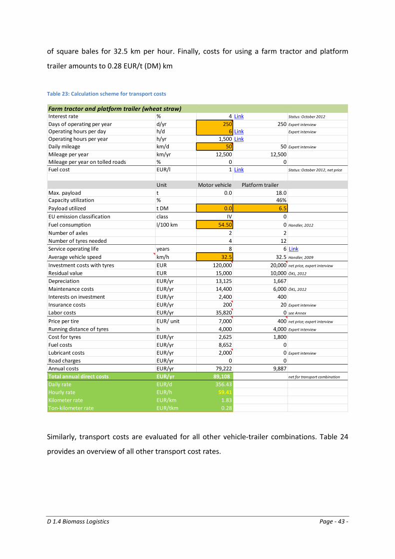
D 1.4 Biomass Logistics Page - 43 -
of square bales for 32.5 km per hour. Finally, costs for using a farm tractor and platform
trailer amounts to 0.28 EUR/t (DM) km
Table 23: Calculation scheme for transport costs
Similarly, transport costs are evaluated for all other vehicle-trailer combinations. Table 24
provides an overview of all other transport cost rates.
Farm tractor and platform trailer (wheat straw)Interest rate % 4 Link Status: October 2012
Days of operating per year d/yr 250 250 Expert interview
Operating hours per day h/d 6 Link Expert interview
Operating hours per year h/yr 1,500 LinkDaily mileage km/d 50 50 Expert interview
Mileage per year km/yr 12,500 12,500Mileage per year on tolled roads % 0 0Fuel cost EUR/l 1 Link Status: October 2012, net price
Unit Motor vehicle Platform trailerMax. payload t 0.0 18.0Capacity utilization % 46%Payload utilized t DM 0.0 6.5EU emission classification class IV 0Fuel consumption l/100 km 54.50 0 Handler, 2012
Number of axles 2 2Number of tyres needed 4 12Service operating life years 8 6 LinkAverage vehicle speed km/h 32.5 32.5 Handler, 2009
Investment costs with tyres EUR 120,000 20,000 net price, expert interview
Residual value EUR 15,000 10,000 ÖKL, 2012
Depreciation EUR/yr 13,125 1,667Maintenance costs EUR/yr 14,400 6,000 ÖKL, 2012
Interests on investment EUR/yr 2,400 400Insurance costs EUR/yr 200 20 Expert interview
Labor costs EUR/yr 35,820 0 see Annex
Price per tire EUR/ unit 7,000 400 net price; expert interview
Running distance of tyres h 4,000 4,000 Expert interview
Cost for tyres EUR/yr 2,625 1,800Fuel costs EUR/yr 8,652 0Lubricant costs EUR/yr 2,000 0 Expert interview
Road charges EUR/yr 0 0Annual costs EUR/yr 79,222 9,887Total annual direct costs EUR/yr 89,108 net for transport combination
Daily rate EUR/d 356.43Hourly rate EUR/h 59.41Kilometer rate EUR/km 1.83Ton-kilometer rate EUR/tkm 0.28
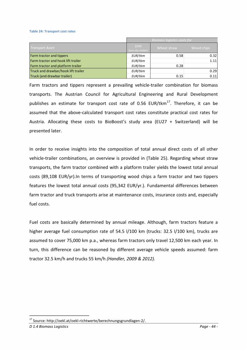
D 1.4 Biomass Logistics Page - 44 -
Table 24: Transport cost rates
Farm tractors and tippers represent a prevailing vehicle-trailer combination for biomass
transports. The Austrian Council for Agricultural Engineering and Rural Development
publishes an estimate for transport cost rate of 0.56 EUR/tkm17. Therefore, it can be
assumed that the above-calculated transport cost rates constitute practical cost rates for
Austria. Allocating these costs to BioBoost’s study area (EU27 + Switzerland) will be
presented later.
In order to receive insights into the composition of total annual direct costs of all other
vehicle-trailer combinations, an overview is provided in (Table 25). Regarding wheat straw
transports, the farm tractor combined with a platform trailer yields the lowest total annual
costs (89,108 EUR/yr).In terms of transporting wood chips a farm tractor and two tippers
features the lowest total annual costs (95,342 EUR/yr.). Fundamental differences between
farm tractor and truck transports arise at maintenance costs, insurance costs and, especially
fuel costs.
Fuel costs are basically determined by annual mileage. Although, farm tractors feature a
higher average fuel consumption rate of 54.5 l/100 km (trucks: 32.5 l/100 km), trucks are
assumed to cover 75,000 km p.a., whereas farm tractors only travel 12,500 km each year. In
turn, this difference can be reasoned by different average vehicle speeds assumed: farm
tractor 32.5 km/h and trucks 55 km/h (Handler, 2009 & 2012).
17 Source: http://oekl.at/oekl-richtwerte/berechnungsgrundlagen-2/.
Unit(tons dry matter)
Wheat straw Wood chips
Farm tractor and tippers EUR/tkm 0.58 0.32Farm tractor and hook lift trailer EUR/tkm 1.11Farm tractor and platform trailer EUR/tkm 0.28Truck and drawbar/hook lift trailer EUR/tkm 0.29Truck (and drawbar trailer) EUR/tkm 0.15 0.11
Biomass logistics costs for
Transport Asset
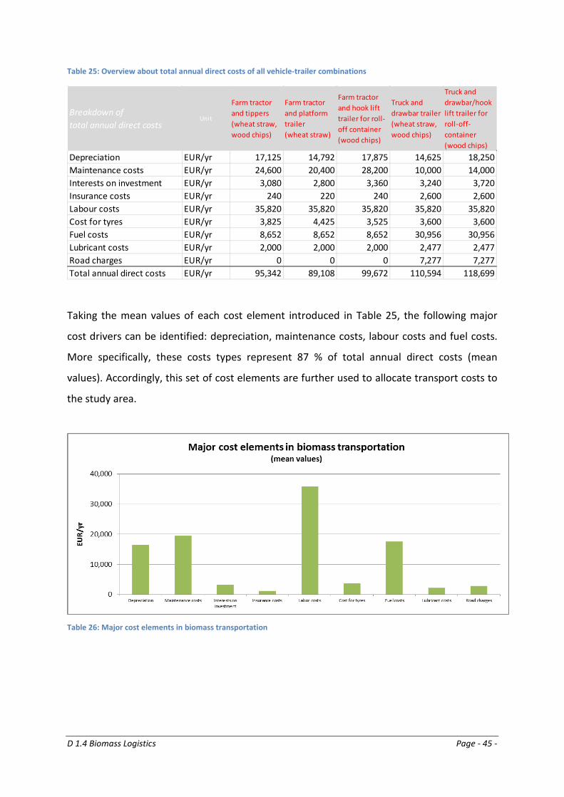
D 1.4 Biomass Logistics Page - 45 -
Table 25: Overview about total annual direct costs of all vehicle-trailer combinations
Taking the mean values of each cost element introduced in Table 25, the following major
cost drivers can be identified: depreciation, maintenance costs, labour costs and fuel costs.
More specifically, these costs types represent 87 % of total annual direct costs (mean
values). Accordingly, this set of cost elements are further used to allocate transport costs to
the study area.
Table 26: Major cost elements in biomass transportation
Breakdown of total annual direct costs
Unit
Farm tractor and tippers (wheat straw, wood chips)
Farm tractor and platform trailer(wheat straw)
Farm tractor and hook lift trailer for roll-off container (wood chips)
Truck and drawbar trailer (wheat straw, wood chips)
Truck and drawbar/hook lift trailer for roll-off-container (wood chips)
Depreciation EUR/yr 17,125 14,792 17,875 14,625 18,250Maintenance costs EUR/yr 24,600 20,400 28,200 10,000 14,000Interests on investment EUR/yr 3,080 2,800 3,360 3,240 3,720Insurance costs EUR/yr 240 220 240 2,600 2,600Labour costs EUR/yr 35,820 35,820 35,820 35,820 35,820Cost for tyres EUR/yr 3,825 4,425 3,525 3,600 3,600Fuel costs EUR/yr 8,652 8,652 8,652 30,956 30,956Lubricant costs EUR/yr 2,000 2,000 2,000 2,477 2,477Road charges EUR/yr 0 0 0 7,277 7,277Total annual direct costs EUR/yr 95,342 89,108 99,672 110,594 118,699
D 1.4 Biomass Logistics Page - 46 -
4.4.2 Handling Costs
Four different handling assets are investigated in this report: (i) front-end loader (farm
tractor), (ii) telescopic handler, (iii) forklift truck, and (iv) gantry crane. In order to evaluate
this equipment, hourly cost rates (EUR/h) are calculated. Table 27 provides an insight into
the calculation scheme.
Handling assets are evaluated based on fixed and variable costs. Figures are primarily taken
from existing studies. For instance, a telescopic handler costs 34.85 EUR each hour. Besides
that costs also idle times (waiting costs) of vehicle-trailer combination need to be
considered. In general, hourly distance fixed costs (DFC) are taken for waiting costs. Then,
performance-related data determined for wheat straw and wood chips, respectively.
Generally, all four handling assets feature a lead time per handling process of 1.5 minutes.
The handling capacity (indicated as tons dry matter) which can be transferred within this
lead time complies with assumed number of loaded square bales or lifting capacity (m³) of
the shovel. Similar to transport assets, handling capacity of handling equipment is restricted
rather by cargo space (m³) than by cargo weight.
Subsequently, two lead times are calculated: lead time I and lead time II. The former implies
the time needed to load or unload a vehicle-trailer combination (min/vehicle), whereas the
latter indicates the time required for transferring one ton (DM) of biogenic residues (min/t
DM). Lead time II also represents the key figure for determining the handling costs (EUR/t
(DM)).
Starting from a fully utilized payload of each investigated transport asset (Table 14, t DM
(100%)), productivity (t DM/h) for each handling asset can be determined. Taking both
hourly cost rates as already described and productivity rates, handling costs (EUR/t DM) can
be defined for each handling equipment and vehicle-trailer combination. Furthermore,
simple stock transfers, which do not consider a waiting vehicle-trailer combination, are
evaluated.
In addition to the four handling assets, tipping process as well as handling roll-off containers
are evaluated. Here, a lead time per handling process of 2.5 minutes is assumed.
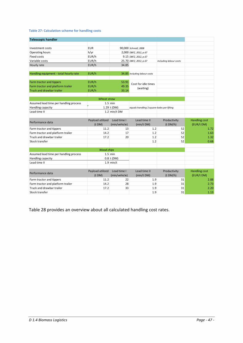
D 1.4 Biomass Logistics Page - 47 -
Table 27: Calculation scheme for handling costs
Table 28 provides an overview about all calculated handling cost rates.
Telescopic handler
Investment costs EUR 90,000 Schnedl, 2008
Operating hours h/yr 2,000 DBFZ, 2012, p.67
Fixed costs EUR/h 9.15 DBFZ, 2012, p.67
Variable costs EUR/h 25.70 DBFZ, 2012, p.67 including labour costs
Hourly rate EUR/h 34.85
Handling equipment - total hourly rate EUR/h 34.85 including labour costs
Farm tractor and tippers EUR/h 53.91Farm tractor and platform trailer EUR/h 49.35Truck and drawbar trailer EUR/h 33.14
Assumed lead time per handling process 1.5 minHandling capacity 1.29 t (DM) equals handling 3 square bales per lifting
Lead time II 1.2 min/t DM
Performance dataPayload utilized
(t DM)Lead time I
(min/vehicle)Lead time II(min/t DM)
Productivity(t DM/h)
Handling cost (EUR/t DM)
Farm tractor and tippers 11.2 13 1.2 52 1.72Farm tractor and platform trailer 14.2 17 1.2 52 1.63Truck and drawbar trailer 17.2 20 1.2 52 1.32Stock transfer 1.2 52 0.68
Assumed lead time per handling process 1.5 minHandling capacity 0.8 t (DM)Lead time II 1.9 min/t
Performance dataPayload utilized
(t DM)Lead time I
(min/vehicle)Lead time II(min/t DM)
Productivity(t DM/h)
Handling cost (EUR/t DM)
Farm tractor and tippers 11.2 22 1.9 31 2.88Farm tractor and platform trailer 14.2 28 1.9 31 2.73Truck and drawbar trailer 17.2 33 1.9 31 2.20Stock transfer 1.9 31 1.13
Cost for idle times (waiting)
Wheat straw
Wood chips
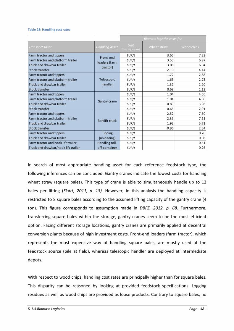
D 1.4 Biomass Logistics Page - 48 -
Table 28: Handling cost rates
In search of most appropriate handling asset for each reference feedstock type, the
following inferences can be concluded. Gantry cranes indicate the lowest costs for handling
wheat straw (square bales). This type of crane is able to simultaneously handle up to 12
bales per lifting (Skøtt, 2011, p. 13). However, in this analysis the handling capacity is
restricted to 8 square bales according to the assumed lifting capacity of the gantry crane (4
ton). This figure corresponds to assumption made in DBFZ, 2012, p. 68. Furthermore,
transferring square bales within the storage, gantry cranes seem to be the most efficient
option. Facing different storage locations, gantry cranes are primarily applied at decentral
conversion plants because of high investment costs. Front-end loaders (farm tractor), which
represents the most expensive way of handling square bales, are mostly used at the
feedstock source (pile at field), whereas telescopic handler are deployed at intermediate
depots.
With respect to wood chips, handling cost rates are principally higher than for square bales.
This disparity can be reasoned by looking at provided feedstock specifications. Logging
residues as well as wood chips are provided as loose products. Contrary to square bales, no
Transport Asset Handling Asset Unit(tons dry matter)
Wheat straw Wood chips
Farm tractor and tippers EUR/t 3.66 7.23Farm tractor and platform trailer EUR/t 3.53 6.97Truck and drawbar trailer EUR/t 3.06 6.04Stock transfer EUR/t 2.10 4.14Farm tractor and tippers EUR/t 1.72 2.88Farm tractor and platform trailer EUR/t 1.63 2.73Truck and drawbar trailer EUR/t 1.32 2.20Stock transfer EUR/t 0.68 1.13Farm tractor and tippers EUR/t 1.04 4.65Farm tractor and platform trailer EUR/t 1.01 4.50Truck and drawbar trailer EUR/t 0.89 3.98Stock transfer EUR/t 0.65 2.91Farm tractor and tippers EUR/t 2.52 7.50Farm tractor and platform trailer EUR/t 2.39 7.11Truck and drawbar trailer EUR/t 1.92 5.71Stock transfer EUR/t 0.96 2.84Farm tractor and tippers EUR/t 0.20Truck and drawbar trailer EUR/t 0.08Farm tractor and hook lift trailer EUR/t 0.31Truck and drawbar/hook lift trailer EUR/t 0.26
Front-end loaders (farm
tractor)
Forklift truck
Telescopic handler
Gantry crane
Tipping (unloading)
Biomass logistics costs for
Handling roll-off container
D 1.4 Biomass Logistics Page - 49 -
compaction takes place. Consequently, the capacity (tons dry matter) of handling assets is
considerably lower for wood chips than for square bales (see Table 27).
Front-end loaders and fork lift trucks seem to be highly inappropriate due to restricted lifting
capacity. Although telescopic handler and gantry cranes exhibits the same lifting capacity (4
m³), gantry cranes seems to be unattractive, too. This is caused by high hourly costs of this
handling asset (89.64 EUR/h) compared to the hourly cost for a telescopic handler (34.85
EUR/h). This same holds true for simple stock transfers.
However, the lowest handling costs for wood chips feature the manipulation by means of
roll-off containers and the tipping process. This can be traced back to the ability to load and
unload a vast amount of biogenic residues within a short period of time without required
additional handling equipment. Therefore, the following conclusion can be drawn.
Considering transport cost rates as shown in Table 24 vehicles with hook lift trailers for roll-
off containers have a major disadvantage compared to other vehicle-trailer combination in
terms of transport costs. However, this perceived drawback may be compensated by also
incorporating handling costs. This situation clearly shows an increased efficiency and cost
advantage through applying roll-off containers. A further advantage of using roll-off
container for handling is given by higher utilization rates of mobile choppers at roadside
landing (Expert interview 15, 2012).
4.4.3 Storage Costs
In general, inventory holding costs include variable costs (i.e. capital costs18) and fixed costs,
e.g. warehousing, depreciation, insurance, etc. Here, fixed costs are referred to storage costs
and are determined by specifications made in Chapter 4.3.3. Storage costs (EUR/t DM) are
examined for wheat straw (square bales) as well as logging residues/wood chips and for
each storage location. Organic municipal waste is not regarded, because HTC plants are
supposed to be located right next to waste collection yard.
18 Capital costs represent opportunity costs for the capital that is tied up in inventory.
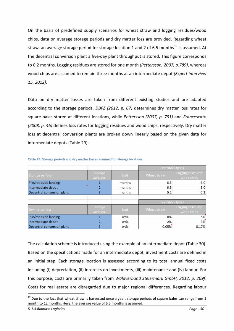
D 1.4 Biomass Logistics Page - 50 -
On the basis of predefined supply scenarios for wheat straw and logging residues/wood
chips, data on average storage periods and dry matter loss are provided. Regarding wheat
straw, an average storage period for storage location 1 and 2 of 6.5 months19 is assumed. At
the decentral conversion plant a five-day plant throughput is stored. This figure corresponds
to 0.2 months. Logging residues are stored for one month (Pettersson, 2007, p.789), whereas
wood chips are assumed to remain three months at an intermediate depot (Expert interview
15, 2012).
Data on dry matter losses are taken from different existing studies and are adapted
according to the storage periods. DBFZ (2012, p. 67) determines dry matter loss rates for
square bales stored at different locations, while Pettersson (2007, p. 791) and Francescato
(2008, p. 46) defines loss rates for logging residues and wood chips, respectively. Dry matter
loss at decentral conversion plants are broken down linearly based on the given data for
intermediate depots (Table 29).
Table 29: Storage periods and dry matter losses assumed for storage locations
The calculation scheme is introduced using the example of an intermediate depot (Table 30).
Based on the specifications made for an intermediate depot, investment costs are defined in
an initial step. Each storage location is assessed according to its total annual fixed costs
including (i) depreciation, (ii) interests on investments, (iii) maintenance and (iv) labour. For
this purpose, costs are primarily taken from Waldverband Steiermark GmbH, 2012, p. 209f.
Costs for real estate are disregarded due to major regional differences. Regarding labour 19 Due to the fact that wheat straw is harvested once a year, storage periods of square bales can range from 1 month to 12 months. Here, the average value of 6.5 months is assumed.
Storage periodsStorage location
Unit Wheat strawLogging residues/
wood chipsPile/roadside landing 1 months 6.5 6.0Intermediate depot 2 months 6.5 3.0Decentral conversion plant 3 months 0.2 0.2
Dry matter lossStorage location
Unit Wheat strawLogging residues/
wood chipsPile/roadside landing 1 wt% 8% 5%Intermediate depot 2 wt% 2% 3%Decentral conversion plant 3 wt% 0.05% 0.17%
Feedstock types
Feedstock types
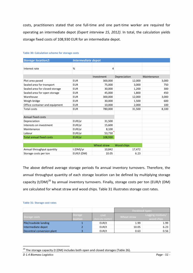
D 1.4 Biomass Logistics Page - 51 -
costs, practitioners stated that one full-time and one part-time worker are required for
operating an intermediate depot (Expert interview 15, 2012). In total, the calculation yields
storage fixed costs of 108,930 EUR for an intermediate depot.
Table 30: Calculation scheme for storage costs
The above defined average storage periods fix annual inventory turnovers. Therefore, the
annual throughput quantity of each storage location can be defined by multiplying storage
capacity (t/DM)20 by annual inventory turnovers. Finally, storage costs per ton (EUR/t (DM)
are calculated for wheat straw and wood chips. Table 31 illustrates storage cost rates.
Table 31: Storage cost rates
20 The storage capacity (t (DM) includes both open and closed storages (Table 26).
Storage location2: Intermediate depot
Interest rate % 4
Investment Depreciation MaintenancePlot area paved EUR 300,000 12,000 3,000 Sealed area for transport EUR 75,000 3,000 750 Sealed area for closed storage EUR 30,000 1,200 300 Sealed area for open storage EUR 45,000 1,800 450 Warehouse EUR 300,000 12,000 3,000 Weigh-bridge EUR 30,000 1,500 600 Office container and equipment EUR 10,000 2,000 100 Total costs EUR 780,000 31,500 8,100
Annual fixed costsDepreciation EUR/yr 31,500 Interests on investment EUR/yr 15,600 Maintenance EUR/yr 8,100 Labour EUR/yr 53,730 Total annual fixed costs EUR/yr 108,930
Wheat straw Wood chipsAnnual throughput quantity t (DM)/yr 10,842 17,472 Storage costs per ton EUR/t (DM) 10.05 6.23
Storage costsStorage location
Unit(tons dry matter)
Wheat strawLogging residues/
wood chipsPile/roadside landing 1 EUR/t 1.99 1.99 Intermediate depot 2 EUR/t 10.05 6.23 Decentral conversion plant 3 EUR/t 0.63 0.56
Feedstock types
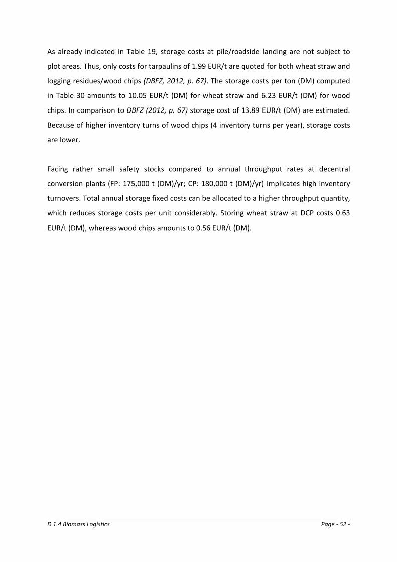
D 1.4 Biomass Logistics Page - 52 -
As already indicated in Table 19, storage costs at pile/roadside landing are not subject to
plot areas. Thus, only costs for tarpaulins of 1.99 EUR/t are quoted for both wheat straw and
logging residues/wood chips (DBFZ, 2012, p. 67). The storage costs per ton (DM) computed
in Table 30 amounts to 10.05 EUR/t (DM) for wheat straw and 6.23 EUR/t (DM) for wood
chips. In comparison to DBFZ (2012, p. 67) storage cost of 13.89 EUR/t (DM) are estimated.
Because of higher inventory turns of wood chips (4 inventory turns per year), storage costs
are lower.
Facing rather small safety stocks compared to annual throughput rates at decentral
conversion plants (FP: 175,000 t (DM)/yr; CP: 180,000 t (DM)/yr) implicates high inventory
turnovers. Total annual storage fixed costs can be allocated to a higher throughput quantity,
which reduces storage costs per unit considerably. Storing wheat straw at DCP costs 0.63
EUR/t (DM), whereas wood chips amounts to 0.56 EUR/t (DM).
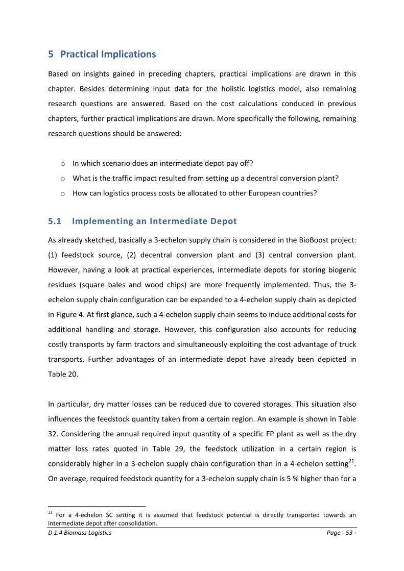
D 1.4 Biomass Logistics Page - 53 -
5 Practical Implications
Based on insights gained in preceding chapters, practical implications are drawn in this
chapter. Besides determining input data for the holistic logistics model, also remaining
research questions are answered. Based on the cost calculations conduced in previous
chapters, further practical implications are drawn. More specifically the following, remaining
research questions should be answered:
o In which scenario does an intermediate depot pay off?
o What is the traffic impact resulted from setting up a decentral conversion plant?
o How can logistics process costs be allocated to other European countries?
5.1 Implementing an Intermediate Depot
As already sketched, basically a 3-echelon supply chain is considered in the BioBoost project:
(1) feedstock source, (2) decentral conversion plant and (3) central conversion plant.
However, having a look at practical experiences, intermediate depots for storing biogenic
residues (square bales and wood chips) are more frequently implemented. Thus, the 3-
echelon supply chain configuration can be expanded to a 4-echelon supply chain as depicted
in Figure 4. At first glance, such a 4-echelon supply chain seems to induce additional costs for
additional handling and storage. However, this configuration also accounts for reducing
costly transports by farm tractors and simultaneously exploiting the cost advantage of truck
transports. Further advantages of an intermediate depot have already been depicted in
Table 20.
In particular, dry matter losses can be reduced due to covered storages. This situation also
influences the feedstock quantity taken from a certain region. An example is shown in Table
32. Considering the annual required input quantity of a specific FP plant as well as the dry
matter loss rates quoted in Table 29, the feedstock utilization in a certain region is
considerably higher in a 3-echelon supply chain configuration than in a 4-echelon setting21.
On average, required feedstock quantity for a 3-echelon supply chain is 5 % higher than for a
21 For a 4-echelon SC setting it is assumed that feedstock potential is directly transported towards an intermediate depot after consolidation.
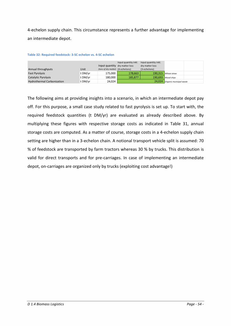
D 1.4 Biomass Logistics Page - 54 -
4-echelon supply chain. This circumstance represents a further advantage for implementing
an intermediate depot.
Table 32: Required feedstock: 3-SC echelon vs. 4-SC echelon
The following aims at providing insights into a scenario, in which an intermediate depot pay
off. For this purpose, a small case study related to fast pyrolysis is set up. To start with, the
required feedstock quantities (t DM/yr) are evaluated as already described above. By
multiplying these figures with respective storage costs as indicated in Table 31, annual
storage costs are computed. As a matter of course, storage costs in a 4-echelon supply chain
setting are higher than in a 3-echelon chain. A notional transport vehicle split is assumed: 70
% of feedstock are transported by farm tractors whereas 30 % by trucks. This distribution is
valid for direct transports and for pre-carriages. In case of implementing an intermediate
depot, on-carriages are organized only by trucks (exploiting cost advantage!)
Annual throughputs UnitInput quantity (tons of dry matter)
Input quantity inkl. dry matter loss (4-echelons)
Input quantity inkl. dry matter loss (3-echelons)
Fast Pyrolysis t DM/yr 175,000 178,663 190,315 Wheat straw
Catalytic Pyrolysis t DM/yr 180,000 185,877 190,693 Wood chips
Hydrothermal Carbonization t DM/yr 24,024 Organic municipal waste24,024
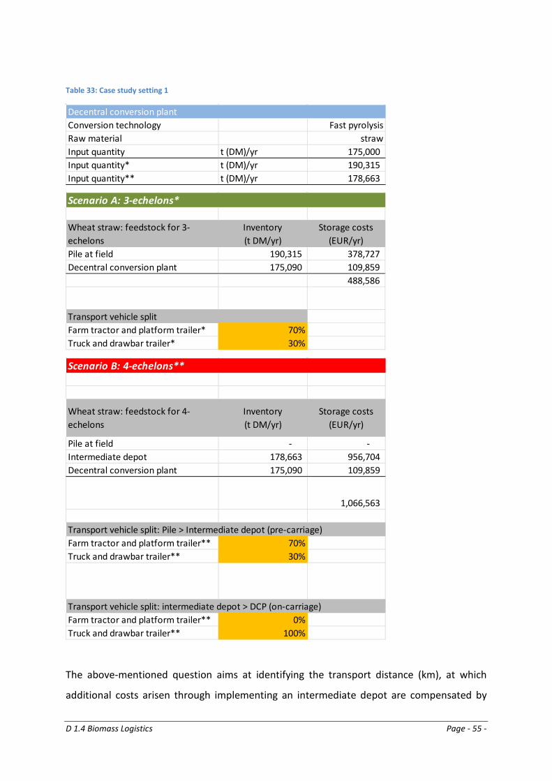
D 1.4 Biomass Logistics Page - 55 -
Table 33: Case study setting 1
The above-mentioned question aims at identifying the transport distance (km), at which
additional costs arisen through implementing an intermediate depot are compensated by
Decentral conversion plantConversion technology Fast pyrolysisRaw material strawInput quantity t (DM)/yr 175,000 Input quantity* t (DM)/yr 190,315 Input quantity** t (DM)/yr 178,663
Scenario A: 3-echelons*
Wheat straw: feedstock for 3-echelons
Inventory(t DM/yr)
Storage costs(EUR/yr)
Pile at field 190,315 378,727 Decentral conversion plant 175,090 109,859
488,586
Transport vehicle splitFarm tractor and platform trailer* 70%Truck and drawbar trailer* 30%
Scenario B: 4-echelons**
Wheat straw: feedstock for 4-echelons
Inventory(t DM/yr)
Storage costs(EUR/yr)
Pile at field - - Intermediate depot 178,663 956,704 Decentral conversion plant 175,090 109,859
1,066,563
Transport vehicle split: Pile > Intermediate depot (pre-carriage)Farm tractor and platform trailer** 70%Truck and drawbar trailer** 30%
Transport vehicle split: intermediate depot > DCP (on-carriage)Farm tractor and platform trailer** 0%Truck and drawbar trailer** 100%
D 1.4 Biomass Logistics Page - 56 -
cost advantages of truck transports; provided that the above depicted transport vehicle split
holds. Therefore, some further assumptions are made in order to finally draw conclusions.
Based on first results of WP1 an average biomass density of 67 tons per km² is assumed.
Considering the required feedstock quantities for a FP plant for the individual scenario (3-
echelon vs. 4-echelon SC), a catchment area of 2,850 km² and 2,675 km² is calculated. For
the sake of simplicity, it is assumed that the catchment area is quadratic. Therefore, the
average transport distance (including 50 % back hauls) can be defined by extracting the
route of the catchment area (DBFZ, 2012, p. 70f). The average transport distance for a 3-
echelon SC amounts to 53 km, whereas a 4-echelon supply chain exhibits 52 km (due to the
individual feedstock quantities). However, the latter features a split transport: pre- and on-
carriages. Assuming that on-carriages are given by 52 km, pre-carriage distances need to be
added. In doing so, the same procedure as for FP plants is applied for intermediate depots.
Again, an average biomass density of 67 tons per km² and an annual throughput quantity of
10,842 t DM/ yr (Table 30) are given. By means of these figures, an average transport
distance of 13 km can be calculated. In total, a transport distance of a 4-echelon SC of 64 km
is yielded. Finally, a simple heuristic is derived: 20% of transport distances relate to pre-
carriages and 80 % of transport distances are on-carriages. Accordingly, this heuristic holds
for the transport distance for a 4-echelon supply chain.
By means of this setting as well as logistics cost rates evaluated before, total logistics costs
including transport, storage and handling are computed (numerical results see annex). In
doing so, the logistics costs as indicated in the logistics reference pathways are taken. In
particular, these pathways determine the logistics equipment (handling assets, etc.) used.
Comparing both scenarios the following chart can be drawn (Figure 8). Logistics costs per ton
as a function of transport distances are calculated. The additional costs of implementing an
intermediate depot favours a 3-SC-echelon until a total transport distance of 80 km. Right at
this specific kilometrage, the cost advantage of truck transportation can be fully exploited.
Therefore, total logistics costs per ton of a 4-echelon SC do not increase as much as of a 3-
echelon SC.
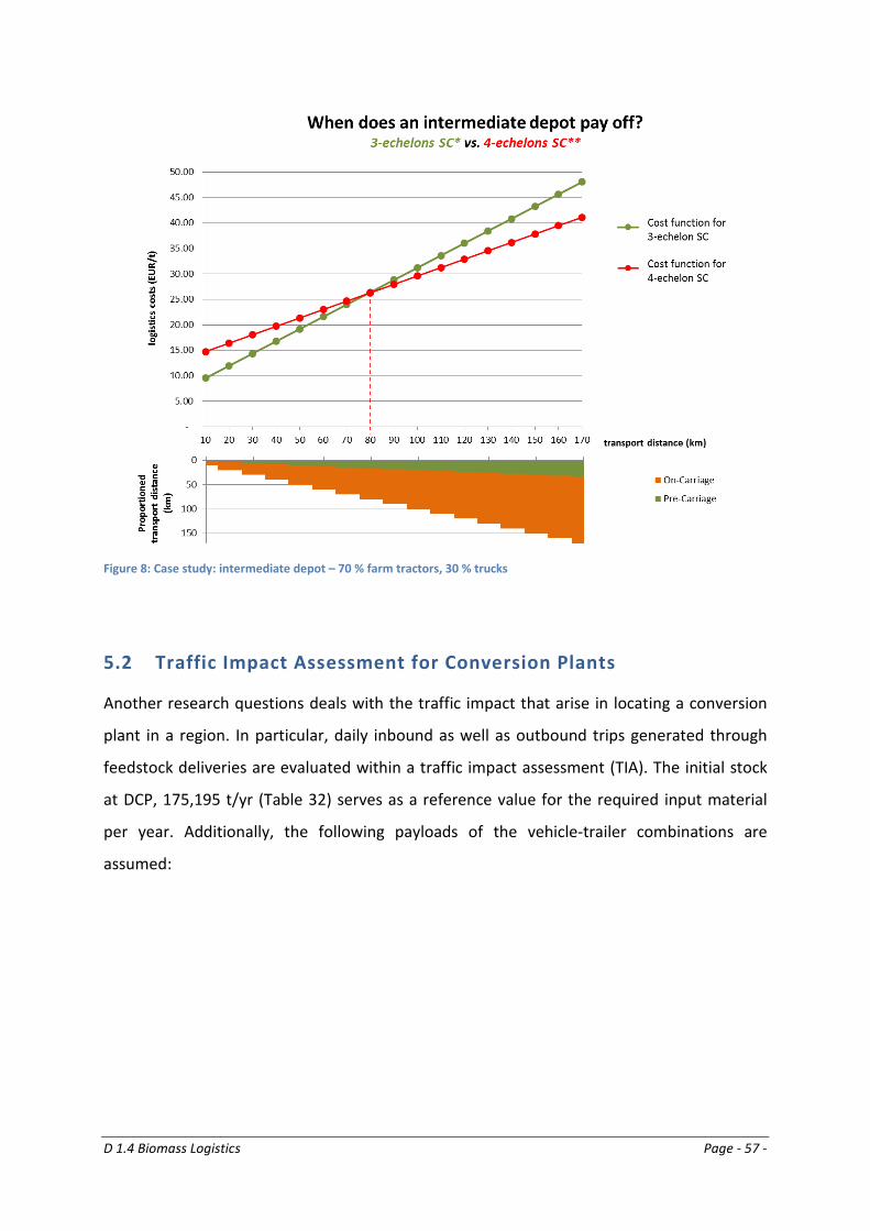
D 1.4 Biomass Logistics Page - 57 -
Figure 8: Case study: intermediate depot – 70 % farm tractors, 30 % trucks
5.2 Traffic Impact Assessment for Conversion Plants
Another research questions deals with the traffic impact that arise in locating a conversion
plant in a region. In particular, daily inbound as well as outbound trips generated through
feedstock deliveries are evaluated within a traffic impact assessment (TIA). The initial stock
at DCP, 175,195 t/yr (Table 32) serves as a reference value for the required input material
per year. Additionally, the following payloads of the vehicle-trailer combinations are
assumed:
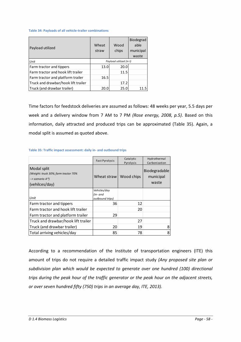
D 1.4 Biomass Logistics Page - 58 -
Table 34: Payloads of all vehicle-trailer combinations
Time factors for feedstock deliveries are assumed as follows: 48 weeks per year, 5.5 days per
week and a delivery window from 7 AM to 7 PM (Rose energy, 2008, p.5). Based on this
information, daily attracted and produced trips can be approximated (Table 35). Again, a
modal split is assumed as quoted above.
Table 35: Traffic impact assessment: daily in- and outbound trips
According to a recommendation of the Institute of transportation engineers (ITE) this
amount of trips do not require a detailed traffic impact study (Any proposed site plan or
subdivision plan which would be expected to generate over one hundred (100) directional
trips during the peak hour of the traffic generator or the peak hour on the adjacent streets,
or over seven hundred fifty (750) trips in an average day, ITE, 2013).
Payload utilizedWheat straw
Wood chips
Biodegradable
municipal waste
Unit
Farm tractor and tippers 13.0 20.0Farm tractor and hook lift trailer 11.5Farm tractor and platform trailer 16.5Truck and drawbar/hook lift trailer 17.2Truck (and drawbar trailer) 20.0 25.0 11.5
Payload utilized (in t)
Fast Pyrolysis Catalytic Pyrolysis
Hydrothermal Carbonization
Modal split (Weight: truck 30%; farm tractor 70%
--> scenario A*)
(vehilces/day)
Wheat straw Wood chipsBiodegradable
municipal waste
Unit
Vehicles/day (in- and outbound trips)
Farm tractor and tippers 36 12Farm tractor and hook lift trailer 20Farm tractor and platform trailer 29Truck and drawbar/hook lift trailer 27Truck (and drawbar trailer) 20 19 8Total arriving vehicles/day 85 78 8
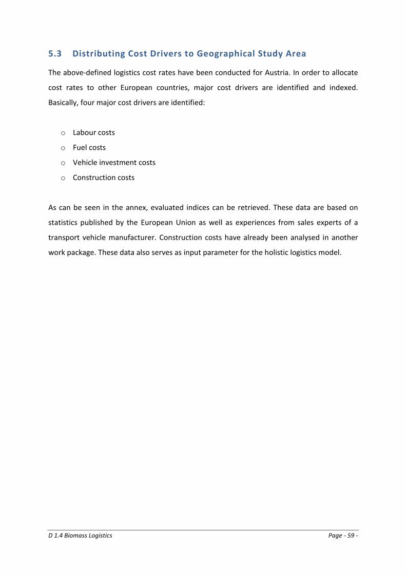
D 1.4 Biomass Logistics Page - 59 -
5.3 Distributing Cost Drivers to Geographical Study Area
The above-defined logistics cost rates have been conducted for Austria. In order to allocate
cost rates to other European countries, major cost drivers are identified and indexed.
Basically, four major cost drivers are identified:
o Labour costs
o Fuel costs
o Vehicle investment costs
o Construction costs
As can be seen in the annex, evaluated indices can be retrieved. These data are based on
statistics published by the European Union as well as experiences from sales experts of a
transport vehicle manufacturer. Construction costs have already been analysed in another
work package. These data also serves as input parameter for the holistic logistics model.
D 1.4 Biomass Logistics Page - 60 -
6 Conclusions and Outlook
This report is primarily dedicated to design and evaluate processes in the field of biomass
logistics. Information based on existing literature as well as implicit, not published, practical
knowledge on manipulating biomass are consolidated and investigated through different
calculations. Finally, key implications are drawn.
First, relevant transport, handling and storage assets are determined. Hereby, plenty of
expert interviews are conducted. By virtue of these specifications, cost calculations are run
in a second step in order to derive target metrics. Generally, farm tractors features higher
costs compared to trucks with respect to transports. This can be reasoned by performance
data and the fact that this type of transport means is not exclusively dedicated for
transports. However, as interviews with practitioners showed, the usage of farm tractors is
prevalent in practice (partially due to a lack of investments in trucks).
Referring to handling, four different assets are investigated: (1) farm tractor with front
loader, (2) forklift truck, (3) telescopic handler and (4) gantry crane. Additionally, loading and
unloading of roll-off containers as well as tipping activities are evaluated. In doing so, some
preferential handling assets are identified for each reference feedstock type.
The storage process is analysed by specifying proper assets, evaluating costs and setting up a
case study. This case study is dedicated to the question: in which scenario does an
intermediate depot pay off? More specifically, two supply chain configurations, i.e. 3-
echelon SC and 4-echelon SC including an intermediate gathering point, are evaluated and
compared. This analysis shows that at a certain transport distance, an intermediate depot
pays off because the cost advantage of trucks can be exploited to a greater extent.
A final assessment about trips generated through locating a conversion plant concluded that
the currently assumed scales of conversion plants are not subject to any further traffic
impact study.
Subsequently, these results serve as input data for both a techno-economic, social and
environmental assessment of complete chains conducted in WP6 as well as ongoing
D 1.4 Biomass Logistics Page - 61 -
activities in WP4. More specifically, the simulation-based optimization model is fed with key
figures generated in this report.
Based on the findings within this report, the energy carrier logistics will be investigated in
the following months and finalized in D4.1 Logistics Concept (due date: project month 15).
Here, especially railway transports as well as inland waterway transports are analysed.
Applying these two transport modes in context of direct transports, transport cost savings
compared to truck transports are likely.
D 1.4 Biomass Logistics Page - 62 -
7 List of References
The following references refer to both the report in hand and the aligned excel file
LogisticsProcesses.xlsx.
AGRAR PLUS GmbH. 2007. Aufbringungspotential von Stroh.
AVA-CO2 Schweiz AG. 2010. Questions & Answers Hydrothermal Carbonisation (HTC).
AVE Österreich GmbH. 2012. Logistik innerhalb der AVE Gruppe - Behälterübersicht.
AVE Österreich GmbH. 2012. Logistik innerhalb der AVE Gruppe - Fahrzeugübersicht.
Bayrische Staatsforsten AöR. 2012. Grundsätze zur Lagerung von Waldhackschnitzeln.
2011. BiG Pack. Großpackenpressen.
Bernard Krone GmbH & Co KG. 2012. BiG Pack Großpackenpressen.
Biogas Forum Bayern. 2010. Biomassetransporte. Hinweise zur Organisation und Verrechnung.
Biogas Forum Bayern. 2010. Verfahren zum Transport von Biomasse.
Biogas Forum Bayern. 2010. Verfahrensalternativen für Biomassetransporte.
Biomass Energy Europe. 2010. Status of Biomass Resource Assessments Version 3.
Blauwens, G.; Baere, P. De; van de Voorde, E. 2008. Transport economics.
BOKU - Universität für Bodenkultur Wien. Waldhackguterzeugung aus Schlagrücklass.
BOKU - Universität für Bodenkultur Wien. 2007. Optimierung der Beschaffungs- und Distributionslogistik
bei großen Biogasanlagen.
BOKU - Universität für Bodenkultur Wien. 2010. Ackerbauliche Ernterückstände als Ressource für
Bioraffinerien - Potentiale und Einschränkungen.
Brainbows. 2007. Biomasse-Ressourcenpotential in Österreich.
Brandt, P. 2007. Die "Hydrothermale Carbonisierung": eine bemerkenswerte Möglichkeit, um die
Entstehung von CO2 zu minimieren oder gar zu vermeiden?
Brassington, B. 2012. Safe Handling of Tank Containers.
Buehler, G. 2005. Verkehrsmittelwahl im Güterverkehr.
D 1.4 Biomass Logistics Page - 63 -
Bundesministerium für Land-und Forstwirtschaft, Umwelt und Wasserwirtschaft. 2012. Federal Waste
Management Plan 2011.
Caputo, A. C. et al. 2005. Economics of biomass energy utilization in combustion and gasification plants:
effects of logistic variables.
CARMEN. 2007. Richtiges Lagern von Hackschnitzeln für Heizwerke: Vermeidung von Bränden durch
Selbstentzündung.
CNH Österreich GmbH. 2012. LRZ-Frontlader.
Commission of the European Communities. 2005. Communication from the Commission - Biomass
action plan.
Conversion and Resource Evaluation LTD. 2001. Transport, Storage and Handling of Biomass Derived
Fast Pyrolysis Liquids.
Danzas Lotse. 2004. Der Logistikbegriff und die drei Bedeutungen der Logistik.
DBFZ – Deutsches Biomasse Forschungs Zentrum. 2012. Basisinformationen für eine nachhaltige
Nutzung von landwirtschaftlichen Reststoffen zur Bioenergiebereitstellung.
Döring, G. 2012. Verfahren zur Ernte und Transport von Biomasse.
Eder, G. 2013. Die Situation der energetischen Nutzung von Stroh in Österreich.
Edwards, M. 2012. Traffic Impact Analysis.
Evonik Industries. 2010. Traffic Assessment.
F.X. Meiller GmbH & Co KG. 2012. Technische Daten Behälter-Transportanhänger.
Fliegl Agro-Center GmbH. 2012. Geräteprogramm.
FNR - Fachagentur Nachwachsende Rohstoffe. 2005. Leitfaden Bioenergie - Planung, Betrieb und
Wirtschaftlichkeit von Bioenergieanlagen.
Francescato, V. et al. 2007. Wood Fuels Handbook. Production, Quality Requirements, Trading.
Francescato, V. et al. 2008. Wood Fuels Handbook. Production, Quality requirements, Trading.
Freppaz, D.; Minciardi, R.; Robba, M.; Rovatti, M.; Sacile, R.; Taramasso, A. 2004. Optimizing forest
biomass exploitation for energy supply at a regional level.
Fritz Voith GmbH. 2012. Greiferkran. Projekt: Danish Crane Building.
D 1.4 Biomass Logistics Page - 64 -
Gleissner, H.; Möller, K. 2009. Fallstudien Logistik. Logistikwissen in der praktischen Anwendung.
Gold, S.; Seuring, S. 2011. Supply chain and logistics issues of bio-energy production.
Hamelinck, C. N.; Suurs, R. A.A; Faaij, A. P.C. 2005. International bioenergy transport costs and energy
balance.
Handler, F. 2011. Ansätze zum Sprit sparen im Ackerbau und in der Grünlandbewirtschaftung.
Handler, F.; Blumauer, E. 2009. Analysis of Working Time Requirement and Logistics for Harvesting Short
Rotation Forestry.
Handler, F.; Blumauer, E. 2010. Logistics chains for wood chips from short rotation forestry.
Heinek, S. 2012. Biomasse Konditionierung. Untersuchung von lagerungsbedingten Biomasseverlusten.
Hernandez, I.; et al. 2012. BioBoost Deliverable D6.1 - Data sheet for assessment.
IEA - International Energy Agency. 2007. Bioenergy Project Development and Biomass Supply - Good
Practice Guidelines.
Kaltschmitt, M.; Hartmann, H.; Hofbauer, H. 2009. Energie aus Biomasse. Grundlagen, Techniken und
Verfahren.
Kühmaier, M. 2008. Optimierung der Waldhackgutbereitstellung auf regionaler Basis.
Land Steiermark. 2007. Untersuchung der Stoffflüsse und sinnvolle Verwertung von sowie
Reststoffnutzung aus Klärschlamm in der Steiermark.
Lang, B. 2012. Woodflow for Austria 2010.
Leible, L. et al. 2005. Entwicklungen von Szenarien über die Bereitstellung von land- und
forstwirtschaftlicher Biomasse in zwei baden-württembergischen Regionen zur Herstellung von
synthetischen Kraftstoffen. Mengenszenarien zur Biomassebereitstellung.
Leible, L. et al. 2006. Kraftstoffproduktion aus Stroh und Waldrestholz - dezentral oder zentral ?
Loeser, M.; Redfern, M.A. 2008. Overview of Biomass Conversion and Generation Technologies.
Loibnegger, T.; Metschina, C. 2010. Biomass Logistic & Trade Centres. 3 Steps for a successful project
realisation.
Lourdes Bravo, M. de; et al. 2011. Key issues of the upstream segment of biofuels supply chain: a
qualitative analysis.
D 1.4 Biomass Logistics Page - 65 -
Mahmudi, H.; Flynn, P. 2006. Rail vs. truck transport of biomass.
Martin, H. 2009. Transport- und Lagerlogistik. Planung, Struktur, Steuerung und Kosten von Systemen
der Intralogistik.
Moser, T. 2012. Standort- und Kapazitätsplanung von BtL-Anlagen in Österreich mittels gemischt-
ganzzahliger Optimierung.
Nicoleit T.; et al. 2012. Charakterisierung von Ethylenglykol-Pyrolysekoks-Slurries, dem Modellbrennstoff
des bioliq®-Vergasers.
OEKL - Österreichisches Kuratorium für Landtechnik und Landentwicklung. 2012. Kraftstoffverbrauch in
der Land- und Forstwirtschaft.
Papacostas, C. S.; Prevedouros, P. D. 2005. Transportation engineering and planning.
Perpiñá, C.; Alfonso, D.; Pérez-Navarro, A.; Peñalvo, E.; Vargas, C.; Cárdenas, R. 2009. Methodology
based on Geographic Information Systems for biomass logistics and transport optimisation.
Pfohl, H.-C. 2010. Logistiksysteme.
Rail Cargo Austria AG. 2010. RCA-Güterwagen. Daten und Details 2010.
Rauch, P.; Gronalt, M.; Häuslmayer, H. 2007. BioLog I. Überregionales Logistik- und
Versorgungsnetzwerk für Holz-Biomasse.
RENEW, Consortium. 2007. Biomass Provision Costs - Final Report.
RENEW, Consortium. 2008. RENEW Final Report.
Rentizelas, A.A; Tatsiopoulos, I.P; Tolis, A. 2009. An optimization model for multi-biomass tri-generation
energy supply.
Riedler-Anhänger GmbH. 2012. Biomasse-Transporter.
Rose Energy. 2008. Transport Assessment / Traffic Impact Assessment.
Schnedl, C. 2008. Energiesysteme der Zukunft - Endbericht. Optimierung der regionalen Warenströme
(Qualitäten, Transport, Aufkommen, etc.) über Biomasse-Logistikzentren.
Schneider, F.; Lebersorger, S. 2009. Untersuchung der Lebensmittel im Restmüll in einer
oberösterreichischen Region.
Schütz GmbH & Co KG. 2012. IBC SX-EX-UL.

D 1.4 Biomass Logistics Page - 66 -
Searcy, E.; et al. 2007. The relative cost of biomass energy transport.
Singh, J.; Panesar, B.S; Sharma, S.K. 2010. A mathematical model for transporting the biomass to
biomass based power plant.
Skøtt, T. 2011. Straw to Energy. Status, Technologies and Innovation in Denmark 2011.
Starkl, F. et al. 2011. Handbuch Intermodaler Verkehr. Kombinierter Verkehr: Schiene - Straße -
Binnenwasserstraße.
Steinmüller, H. 2010. Nachhaltige Bodennutzung in Österreich.
Still. 2012. RX 70 Technical data. Diesel and LPG forklift trucks.
Stolletz, R.; Stolletz, L. 2008. Linearisierungsverfahren für Standortplanungsprobleme mit nichtlinearen
Transportkosten.
Strobl, M. 2012. Biomasse-Ernte-Logistik (BEL). Planzahlen, Methode und Anwendung für den
Praxiseinsatz.
Swissterminal. 2012. Containerübersicht.
Syncom. 2012. Minutes BioBoost Telephone Conference.
The University of Montana. 2011. Draft Transportation Impact Assessment.
Trippe, F. et al. 2010. Techno-Economic Analysis of Fast Pyrolysis as a Process Step within Biomass-to-
Liquid Fuel Production.
Velazquez-Marti, B.; Fernandez-Gonzalez, E. 2010. Mathematical algorithms to locate factories to
transform biomass in bioenergy focused on logistic network construction.
Waldverband Niederösterreich 2012 – Informationsblatt zur Abrechnung von Biomasse": Template
"Bibliography - Unknown - (Default template)" is not defined.]
Waldverband Steiermark GmbH. 2008. Optimierung der regionalen Warenströme über Biomasse-
Logistikzentren.
Weber, J. 2012. Logistikkostenrechnung. Kosten-, Leistungs- und Erlösinformationen zur
erfolgsorientierten Steuerung der Logistik.
WWF Österreich. 2006. Potenziale der Biomassenutzung aus dem Österreichischen Wald unter
Berücksichtigung der Biodiversität.
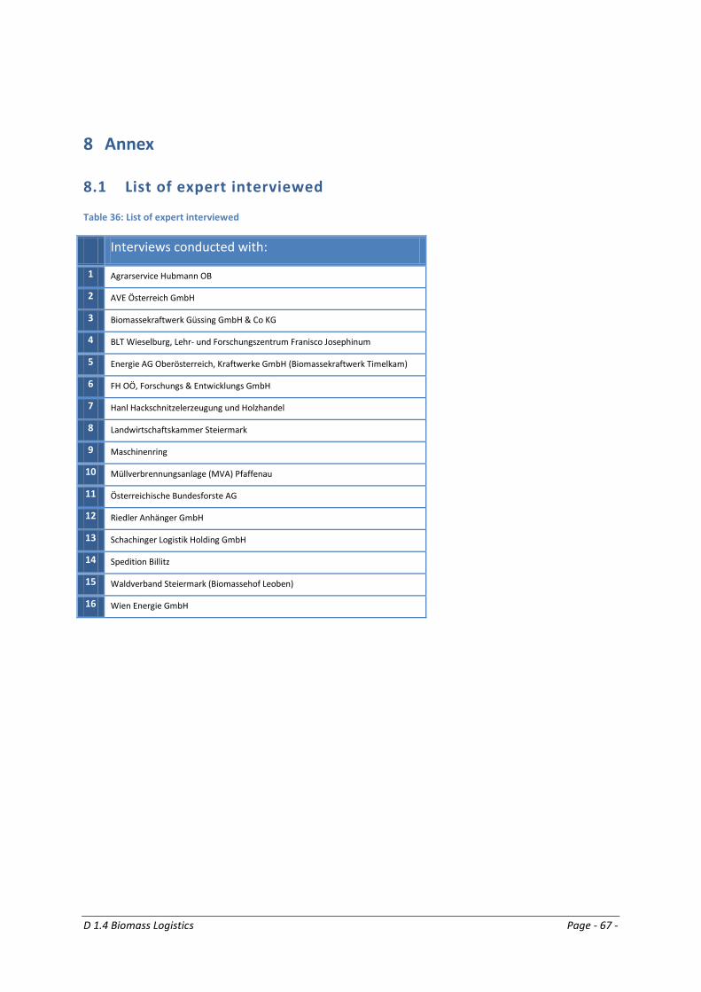
D 1.4 Biomass Logistics Page - 67 -
8 Annex
8.1 List of expert interviewed
Table 36: List of expert interviewed
Interviews conducted with:
1 Agrarservice Hubmann OB
2 AVE Österreich GmbH
3 Biomassekraftwerk Güssing GmbH & Co KG
4 BLT Wieselburg, Lehr- und Forschungszentrum Franisco Josephinum
5 Energie AG Oberösterreich, Kraftwerke GmbH (Biomassekraftwerk Timelkam)
6 FH OÖ, Forschungs & Entwicklungs GmbH
7 Hanl Hackschnitzelerzeugung und Holzhandel
8 Landwirtschaftskammer Steiermark
9 Maschinenring
10 Müllverbrennungsanlage (MVA) Pfaffenau
11 Österreichische Bundesforste AG
12 Riedler Anhänger GmbH
13 Schachinger Logistik Holding GmbH
14 Spedition Billitz
15 Waldverband Steiermark (Biomassehof Leoben)
16 Wien Energie GmbH
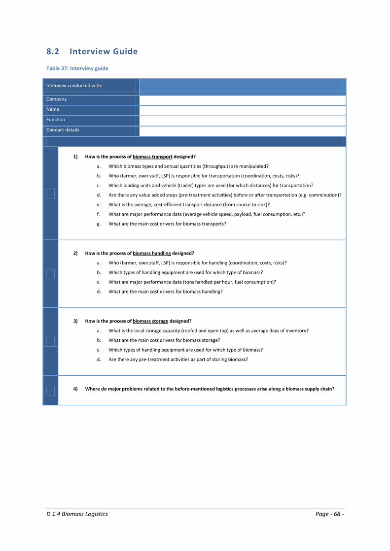
D 1.4 Biomass Logistics Page - 68 -
8.2 Interview Guide
Table 37: Interview guide
Interview conducted with:
Company
Name
Function
Condact details
1) How is the process of biomass transport designed?
a. Which biomass types and annual quantities (throughput) are manipulated?
b. Who (farmer, own staff, LSP) is responsible for transportation (coordination, costs, risks)?
c. Which loading units and vehicle (trailer) types are used (for which distances) for transportation?
d. Are there any value added steps (pre-treatment activities) before or after transportation (e.g. comminution)?
e. What is the average, cost-efficient transport distance (from source to sink)?
f. What are major performance data (average vehicle speed, payload, fuel consumption, etc.)?
g. What are the main cost drivers for biomass transports?
2) How is the process of biomass handling designed?
a. Who (farmer, own staff, LSP) is responsible for handling (coordination, costs, risks)?
b. Which types of handling equipment are used for which type of biomass?
c. What are major performance data (tons handled per hour, fuel consumption)?
d. What are the main cost drivers for biomass handling?
3) How is the process of biomass storage designed?
a. What is the local storage capacity (roofed and open top) as well as average days of inventory?
b. What are the main cost drivers for biomass storage?
c. Which types of handling equipment are used for which type of biomass?
d. Are there any pre-treatment activities as part of storing biomass?
4) Where do major problems related to the before-mentioned logistics processes arise along a biomass supply chain?
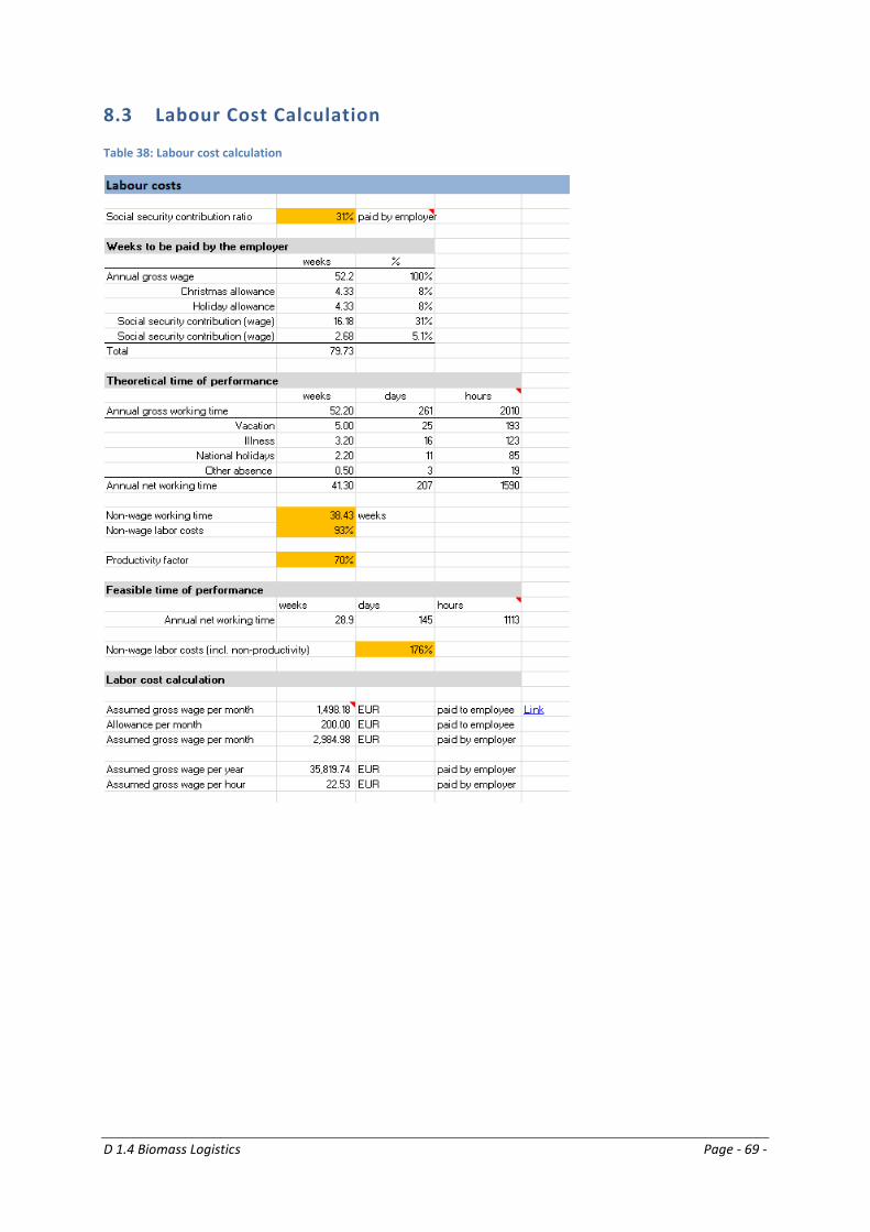
D 1.4 Biomass Logistics Page - 69 -
8.3 Labour Cost Calculation
Table 38: Labour cost calculation
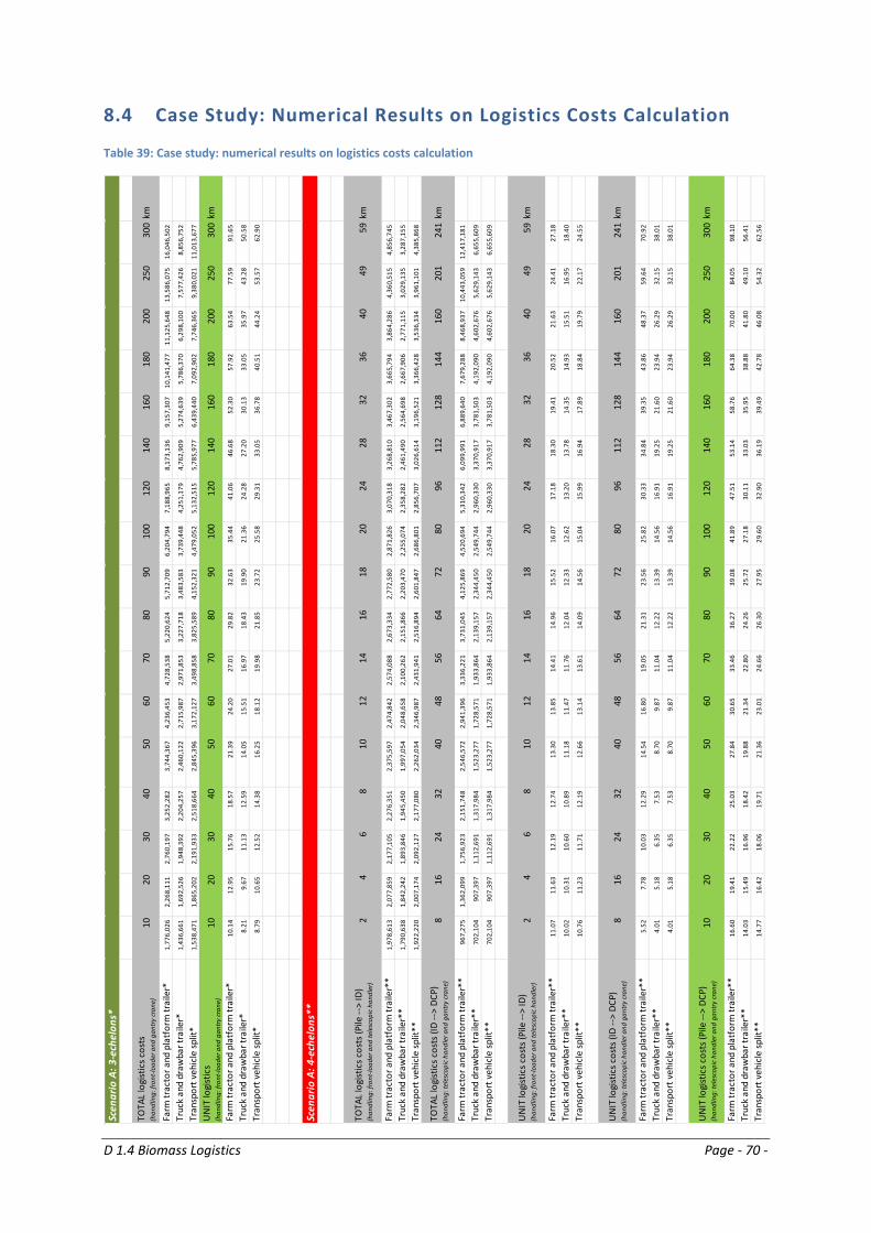
D 1.4 Biomass Logistics Page - 70 -
8.4 Case Study: Numerical Results on Logistics Costs Calculation
Table 39: Case study: numerical results on logistics costs calculation
Scen
ario
A: 3
-ech
elon
s*
TOTA
L lo
gist
ics c
osts
(han
dlin
g: fr
ont-l
oade
r and
gan
try cr
ane)
1020
3040
5060
7080
9010
012
014
016
018
020
025
030
0km
Farm
trac
tor a
nd p
latf
orm
trai
ler*
1,77
6,02
6
2,
268,
111
2,76
0,19
7
3,
252,
282
3,74
4,36
7
4,23
6,45
3
4,
728,
538
5,22
0,62
4
5,
712,
709
6,20
4,79
4
7,
188,
965
8,17
3,13
6
9,
157,
307
10,1
41,4
77
11,1
25,6
48
13,5
86,0
75
16,0
46,5
02
Truc
k an
d dr
awba
r tra
iler*
1,43
6,66
1
1,
692,
526
1,94
8,39
2
2,
204,
257
2,46
0,12
2
2,71
5,98
7
2,
971,
853
3,22
7,71
8
3,
483,
583
3,73
9,44
8
4,
251,
179
4,76
2,90
9
5,
274,
639
5,78
6,37
0
6,
298,
100
7,57
7,42
6
8,
856,
752
Tran
spor
t veh
icle
split
*1,
538,
471
1,86
5,20
2
2,
191,
933
2,51
8,66
4
2,
845,
396
3,
172,
127
3,49
8,85
8
3,
825,
589
4,15
2,32
1
4,
479,
052
5,13
2,51
5
5,
785,
977
6,43
9,44
0
7,
092,
902
7,74
6,36
5
9,
380,
021
11,0
13,6
77
UN
IT lo
gist
ics
(han
dlin
g: fr
ont-l
oade
r and
gan
try cr
ane)
1020
3040
5060
7080
9010
012
014
016
018
020
025
030
0km
Farm
trac
tor a
nd p
latf
orm
trai
ler*
10.1
4
12
.95
15.7
6
18
.57
21.3
9
24
.20
27.0
1
29
.82
32.6
3
35
.44
41.0
6
46
.68
52.3
0
57
.92
63.5
4
77
.59
91.6
5
Truc
k an
d dr
awba
r tra
iler*
8.21
9.
67
11.1
3
12
.59
14.0
5
15
.51
16.9
7
18
.43
19.9
0
21
.36
24.2
8
27
.20
30.1
3
33
.05
35.9
7
43
.28
50.5
8
Tran
spor
t veh
icle
split
*8.
79
10.6
5
12
.52
14.3
8
16
.25
18.1
2
19
.98
21.8
5
23
.72
25.5
8
29
.31
33.0
5
36
.78
40.5
1
44
.24
53.5
7
62
.90
Scen
ario
A: 4
-ech
elon
s**
TOTA
L lo
gist
ics c
osts
(Pile
-->
ID)
(han
dlin
g: fr
ont-l
oade
r and
tele
scop
ic ha
ndle
r)2
46
810
1214
1618
2024
2832
3640
4959
km
Farm
trac
tor a
nd p
latf
orm
trai
ler*
*1,
978,
613
2,07
7,85
9
2,
177,
105
2,27
6,35
1
2,
375,
597
2,
474,
842
2,57
4,08
8
2,
673,
334
2,77
2,58
0
2,
871,
826
3,07
0,31
8
3,
268,
810
3,46
7,30
2
3,
665,
794
3,86
4,28
6
4,
360,
515
4,85
6,74
5
Truc
k an
d dr
awba
r tra
iler*
*1,
790,
638
1,84
2,24
2
1,
893,
846
1,94
5,45
0
1,
997,
054
2,
048,
658
2,10
0,26
2
2,
151,
866
2,20
3,47
0
2,
255,
074
2,35
8,28
2
2,
461,
490
2,56
4,69
8
2,
667,
906
2,77
1,11
5
3,
029,
135
3,28
7,15
5
Tran
spor
t veh
icle
split
**1,
922,
220
2,00
7,17
4
2,
092,
127
2,17
7,08
0
2,
262,
034
2,
346,
987
2,43
1,94
1
2,
516,
894
2,60
1,84
7
2,
686,
801
2,85
6,70
7
3,
026,
614
3,19
6,52
1
3,
366,
428
3,53
6,33
4
3,
961,
101
4,38
5,86
8
TOTA
L lo
gist
ics c
osts
(ID
-->
DCP)
(han
dlin
g: te
lesc
opic
hand
ler a
nd g
antry
cran
e)8
1624
3240
4856
6472
8096
112
128
144
160
201
241
km
Farm
trac
tor a
nd p
latf
orm
trai
ler*
*96
7,27
5
1,36
2,09
9
1,
756,
923
2,15
1,74
8
2,
546,
572
2,
941,
396
3,33
6,22
1
3,
731,
045
4,12
5,86
9
4,
520,
694
5,31
0,34
2
6,
099,
991
6,88
9,64
0
7,
679,
288
8,46
8,93
7
10
,443
,059
12
,417
,181
Truc
k an
d dr
awba
r tra
iler*
*70
2,10
4
907,
397
1,
112,
691
1,31
7,98
4
1,
523,
277
1,
728,
571
1,93
3,86
4
2,
139,
157
2,34
4,45
0
2,
549,
744
2,96
0,33
0
3,
370,
917
3,78
1,50
3
4,
192,
090
4,60
2,67
6
5,
629,
143
6,65
5,60
9
Tran
spor
t veh
icle
split
**70
2,10
4
907,
397
1,
112,
691
1,31
7,98
4
1,
523,
277
1,
728,
571
1,93
3,86
4
2,
139,
157
2,34
4,45
0
2,
549,
744
2,96
0,33
0
3,
370,
917
3,78
1,50
3
4,
192,
090
4,60
2,67
6
5,
629,
143
6,65
5,60
9
UN
IT lo
gist
ics c
osts
(Pile
-->
ID)
(han
dlin
g: fr
ont-l
oade
r and
tele
scop
ic ha
ndle
r)2
46
810
1214
1618
2024
2832
3640
4959
km
Farm
trac
tor a
nd p
latf
orm
trai
ler*
*11
.07
11.6
3
12
.19
12.7
4
13
.30
13.8
5
14
.41
14.9
6
15
.52
16.0
7
17
.18
18.3
0
19
.41
20.5
2
21
.63
24.4
1
27
.18
Truc
k an
d dr
awba
r tra
iler*
*10
.02
10.3
1
10
.60
10.8
9
11
.18
11.4
7
11
.76
12.0
4
12
.33
12.6
2
13
.20
13.7
8
14
.35
14.9
3
15
.51
16.9
5
18
.40
Tran
spor
t veh
icle
split
**10
.76
11.2
3
11
.71
12.1
9
12
.66
13.1
4
13
.61
14.0
9
14
.56
15.0
4
15
.99
16.9
4
17
.89
18.8
4
19
.79
22.1
7
24
.55
UN
IT lo
gist
ics c
osts
(ID
-->
DCP)
(han
dlin
g: te
lesc
opic
hand
ler a
nd g
antry
cran
e)8
1624
3240
4856
6472
8096
112
128
144
160
201
241
km
Farm
trac
tor a
nd p
latf
orm
trai
ler*
*5.
52
7.78
10
.03
12.2
9
14
.54
16.8
0
19
.05
21.3
1
23
.56
25.8
2
30
.33
34.8
4
39
.35
43.8
6
48
.37
59.6
4
70
.92
Truc
k an
d dr
awba
r tra
iler*
*4.
01
5.18
6.
35
7.53
8.
70
9.
87
11.0
4
12
.22
13.3
9
14
.56
16.9
1
19
.25
21.6
0
23
.94
26.2
9
32
.15
38.0
1
Tran
spor
t veh
icle
split
**4.
01
5.18
6.
35
7.53
8.
70
9.
87
11.0
4
12
.22
13.3
9
14
.56
16.9
1
19
.25
21.6
0
23
.94
26.2
9
32
.15
38.0
1
UN
IT lo
gist
ics c
osts
(Pile
-->
DCP)
(han
dlin
g: te
lesc
opic
hand
ler a
nd g
antry
cran
e)10
2030
4050
6070
8090
100
120
140
160
180
200
250
300
km
Farm
trac
tor a
nd p
latf
orm
trai
ler*
*16
.60
19.4
1
22
.22
25.0
3
27
.84
30.6
5
33
.46
36.2
7
39
.08
41.8
9
47
.51
53.1
4
58
.76
64.3
8
70
.00
84.0
5
98
.10
Truc
k an
d dr
awba
r tra
iler*
*14
.03
15.4
9
16
.96
18.4
2
19
.88
21.3
4
22
.80
24.2
6
25
.72
27.1
8
30
.11
33.0
3
35
.95
38.8
8
41
.80
49.1
0
56
.41
Tran
spor
t veh
icle
split
**14
.77
16.4
2
18
.06
19.7
1
21
.36
23.0
1
24
.66
26.3
0
27
.95
29.6
0
32
.90
36.1
9
39
.49
42.7
8
46
.08
54.3
2
62
.56
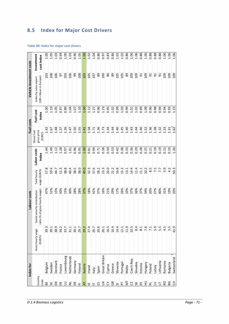
D 1.4 Biomass Logistics Page - 71 -
8.5 Index for Major Cost Drivers
Table 40: Index for major cost drivers
Coun
try
Code
Gros
s hou
rly w
age
(EUR
/h)
Soci
al se
curit
y co
ntrib
utio
n ra
tio (%
of g
ross
hou
rly w
age)
Tota
l hou
rly
wag
e (E
UR/h
)La
bor c
osts
in
dex
Dies
el fu
el
gros
s pric
e (E
UR/l
)
Fuel
cos
t in
dex
Inde
x by
sale
s exp
ert
(100
= M
ean
in E
urop
e)In
vest
men
t co
st in
dex
BEBe
lgiu
m39
.347
%57
.81.
441.
421.
0010
31.
00SE
Swed
en39
.152
%59
.41.
491.
671.
1910
81.
05DK
Denm
ark
38.9
15%
44.7
1.12
1.48
1.05
106
1.03
FRFr
ance
34.2
50%
51.3
1.28
1.37
0.97
970.
94LU
Luxe
mbo
urg
33.7
15%
38.8
0.97
1.26
0.89
103
1.00
NL
Net
herla
nds
31.1
30%
40.4
1.01
1.47
1.04
106
1.03
DEGe
rman
y30
.128
%38
.50.
961.
501.
0799
0.96
FIFi
nlan
d29
.728
%38
.00.
951.
551.
1010
81.
05AT
Aust
ria29
.237
%40
.01.
001.
411.
0010
31.
00IE
Irlan
d27
.418
%32
.30.
811.
581.
1210
51.
02IT
Italy
26.7
41%
37.6
0.94
1.71
1.21
107
1.04
ESSp
ain
20.6
37%
28.2
0.71
1.36
0.96
890.
86U
KGr
eat B
ritai
n20
.116
%23
.30.
581.
731.
2310
00.
97CY
Cypr
us16
.521
%20
.00.
501.
340.
9586
0.83
GRGr
eece
16.4
29%
21.2
0.53
1.44
1.02
890.
86SI
Slov
enia
14.4
17%
16.8
0.42
1.40
0.99
105
1.02
PTPo
rtug
al12
.126
%15
.20.
381.
451.
0310
51.
02M
TM
alta
11.9
10%
13.1
0.33
1.40
0.99
890.
86CZ
Czec
h Re
p.10
.537
%14
.40.
361.
431.
0110
91.
06SK
Slov
akia
8.4
36%
11.4
0.29
1.44
1.02
109
1.06
EEEs
toni
a8.
137
%11
.10.
281.
400.
9991
0.88
HUHu
ngar
y7.
634
%10
.20.
251.
521.
0810
91.
06PL
Pola
nd7.
120
%8.
50.
211.
360.
9691
0.88
LVLa
tvia
5.9
27%
7.5
0.19
1.38
0.98
910.
88LT
Lith
uani
a5.
540
%7.
70.
191.
320.
9491
0.88
RORo
man
ia4.
531
%5.
90.
151.
330.
9410
91.
06BG
Bulg
aria
3.5
19%
4.2
0.10
1.31
0.93
109
1.06
CHSw
itzer
land
41.9
20%
50.3
1.26
1.62
1.15
109
1.06
Labo
ur c
osts
Fuel
cos
tsVe
hicl
e in
vest
men
t cos
tsIn
dex
for