i

Cyber Physical Systems

For

Self-Healing of Smart Grids

A REPORT

Submitted by

Felix Albert Nongneng

In partial fulfilment of the requirement for the degree of

MASTER OF TECHNOLOGY

Guided by

Dr. K. Shanti Swarup

DEPARTMENT OF ELECTRICAL ENGINEERING

INDIAN INSTITUTE OF TECHNOLOGY MADRAS

CHENNAI 600025

JAN 2020

ii

ABSTRACT

Smart grid are complex networks that intensifies the dependence of

power system operation on cyber infrastructure for control and monitoring

purposes. In the applications like wide-area monitoring systems and demand-

side management, power utilities are in the process of re-modelling additional

communication infrastructure to support their operational requirements.

Resiliency is critically important to ensure secure, reliable and economic

operation of the bulk power system. In addition to improving cyber security

of the communication network, it becomes imperative to develop control

system algorithms that are both attack resilient and tolerant. One of the main

features of smart grid is the self –healing capability. According to this feature,

all the new monitoring, communication and control facilities pertaining to

smart grid are deployed resulting in an efficient restoration strategy.

The first system under study, the distribution networks restoration

solution is done by transferring the loads in the off outage area and transferred

to the neighboring feeders through changing the status of normally –closed

(sectionalizing) and normally-open (tie) switches.

The second study case –Six Bus System, a Distributed Denail of

Service Attack (DDOS) is performed where the Attacker inject ‘Attack’ script

into the Communication Layer to infect the Nodes and flood the Server and

the Control Center performing remedial actions by sending a ‘Clean’ script to

clear the faults in these infected Nodes under abnormal conditions. We use

State Estimation algorithm –WLS method as a controller to detect and prevent

bad data injection into the Communication Layer during normal and faulted

scenarios.

The Tools and Software used: ETAP 16.0.0, GNS3, MATLAB,

OPNET Riverbed Modeller Academic Edition.

Keywords: Cyber Physical Systems, Self Healing, Architecture, ICT,

Smart Grid, CPS modelling, DDoS.

iii

TABLE OF CONTENTS

CHAPTER TITLE PAGE NO.

ABSTRACT

i

LIST OF FIGURES v

LIST OF TABLES v

1 PREAMBLE

1.1 INTRODUCTION 1

1.2 SELF-HEALING OF SMART GRID 2

1.3 CPS MODELLING AND ASSESSMENT 3

1.4 FUTURE OUTLOOK OF CPS 4

1.5 ATTACK RESILIENT CONTROL 6

2 POWER SYSTEM NETWORK MODELLING

2.1 SYSTEM UNDER STUDY 7

2.2 PHYSICAL LAYER MODELLING IN ETAP 8

3 PHYSICAL LAYER SIMULATION IN ETAP 16.0.0

3.1 LOAD FLOW ANALYSIS 13

3.2 SHORT CIRCUIT ANALYSIS 18

3.3 INTELLIGENT SWITCHING SEQUENCE

MANAGER

20

4 CYBER PHYSICAL SYSTEM APPLICATION

4.1 MATLAB SIMULINK OF 6 BUS SYSTEM

UNDER STUDY

22

5 STATE ESTIMATION CONTROLLER

5.1 MATLAB CODE FOR STATE ESTIMATION

i) LINE DATAS 23

ii) BUS DATAS 23

iii) MEASUREMENT DATAS 24

iv

iv) POWER SYSTEM STATE

ESTIMATION USING WLS

25-29

5.2 RESULT FOR STATE ESTIMATION OF SIX

BUS SYSTEM

30

6 DESIGN OF COMMUNICATION LAYER

6.1 DESIGN IN GNS3 31

6.2 DESIGN IN RIVERBED MODELLER 32

6.3 DDOS ATTACK ON COMMUNICATION

LAYER

i) NETWORK CONFIGURATION 33

ii) ATTACK AND REMEDY SETTINGS 33

iii) RESULTS 34

6.4 GLOBAL STATISTICS

i) ALL NODES TRAFFIC

SIMULATION RESULT

35

6.5 OBJECT STATISTICS

i) SERVER PERFORMANCE 35

ii) CLIENT SIMULATION RESULTS 36

7 CONCLUSION 37

8 REFERENCES 39

v

LIST OF TABLES

TITLE PAGE

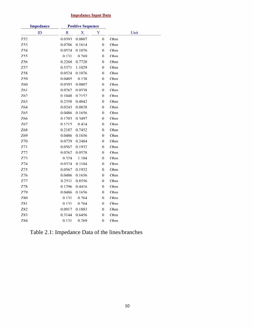
2.1 Impedance Data of lines/branches 9-10

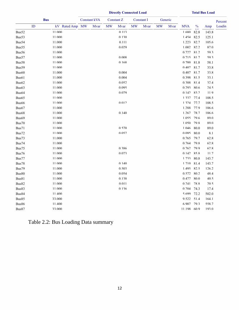
2.2 Bus Loading Data Summary 11-12

3.1 Load Flow Report 14-17

3.3 Short Circuit Analysis Report 19

LIST OF FIGURES

1.3 CPS architecture framework 3

1.4 Future outlook of CPS 5

2.1 Distribution Network of System under Study 7

2.2 Single Line Diagram of System under Study 8

3.1 Load Flow Study for Normal Case 13

3.2 Short Circuit Analysis of Study Case 18

3.3 Switching Sequence in steps in case of fault 20

4.1 SLD of Six Bus System under Study 21

4.2 MATLAB Simulink of Six Bus System 22

6.2 Communication Layer of Six Bus System 32

6.3 Script (Traffic) send by the Attacker 34

6.4 Infected device count and IP traffic dropped

(packets/secs)

35

6.5 Traffic received by Server (packets/secs) 35

6.6 Client Http Object response time and Traffic

received (packets/secs)

36

1

Chapter 1

Preamble

1.1 Introduction

Smart Grid is a power delivery infrastructure which is integrated with two-

way communications and electricity flows, creating an automated, widely

distributed energy delivery network. It can capture and analyze data regarding power

generation, delivery and usage in near real-time by way of advanced sensing

technologies and control methods to help balance power supply and demand.

Compared to traditional power system, Smart Grid has unique properties such as

high efficiency, high reliability and high security.

CPS refers to a class of complex systems that feature tight integration and

coupling of their cyber and physical aspects. The ability to interact with, and expand

the capabilities of, the physical world through Computation, Communication, and

Control is a key enabler for real-time sensing, dynamic control and information

service of large engineering systems. As the evolution of Internet of Things, CPS

can safely, reliably and efficiently monitor or control the physical entities in near

real-time.

Distribution systems consist of groups of interconnected radial circuits. The

configuration may be varied via switching operations to transfer loads among the

feeders. Two types of switches are used in primary distribution systems. They are

normally closed switches (sectionalizing switches) or normally open switches (tie

switches). Both types are designed for both protection and configuration

management. Network reconfiguration is the process of changing the topology of

distribution systems by altering the open/closed status of switches. From the

mathematical programming viewpoint, the restoration problem is a mixed-integer

due to the status of switches and non-linear due to the power flow constraints

optimization problem.

2

1.2 Self -Healing of Smart Grid

Self-healing is the ability of distribution systems to automatically restore

themselves after a faults and in case of an attack like a DDOS attack which can cause

permanent damage to the system. Self-healing plans to isolate the fault and

reenergize the out of-service zones with minimum human intervention, depending

on the level of automation. After locating a fault, optimum restoration scheme

minimize the number of outage zones while satisfying system and operational

constraints. A fully automated self-healing scheme can only applied within a smart

grid context where remote-controlled switching equipment are used for switching

actions to isolate fault, shed or restore loads and change the system topology.

Various studies have been done to address the service restoration problem, in a

centralized or decentralized manner, each has its own pros and cons.

In traditional distribution network, after happening a fault, the upstream

circuit breaker will be opened and shuts down the power on the entire feeder. The

upstream section of fault can be restored after locating fault by manual switching. In

smart grids with advanced distribution automation, the typical steps of fault location,

isolation and service restoration are done to enhance system reliability and reducing

the effect of fault on system. In the proposed method, after isolating fault, a

switching sequence can be done so as to restore as many loads as possible in the

faulty feeder. The reverse switching sequence is applied to the network after the

faulty section is completely repaired. Then the network can return to its pre-fault

configuration.

The self-healing property will lead to a resilient smart grid, which allows

healthy zones to continue operation after a permanent fault. The proposed structure

depends on situation and plans to reenergize the out-of-service zones after locating

a fault and minimize the number of outage zones while satisfying system and

operational constraints. Switching actions are done to isolate fault, shed or restore

loads and change the system topology. The main goal of self-healing in this paper is

to increase reliability of system, minimize out-of-service area after a fault by using

distributed control approaches. In order to make good decision, it is crucial to gather

enough information. Communication is the key in case of fault and DDOS attack in

order to bring back the system to normal stable state. Therefore, proper mapping

between Physical Layer and Communication Layer is very crucial.

3

1.3 CPS Modelling and Assessment

The gradually increasing dependencies of power grid on its information

system, has been confirmed that it has led to many catastrophic blackouts of power

system owing to the failures of information system. It is necessary to establish a

reasonable theoretical analysis and safety assessment method for CPS, which can

provide direction for optimizing the configuration of its cyber side to enhance the

robustness and reliable operation of CPS.

i. Cyber Physical Modeling

CPS modeling is the basis for achieving safety assessment, fault analysis and

optimization. The starting point is to analyze the effect of mutual coupling between

the primary power grid in physical side and the secondary information system in

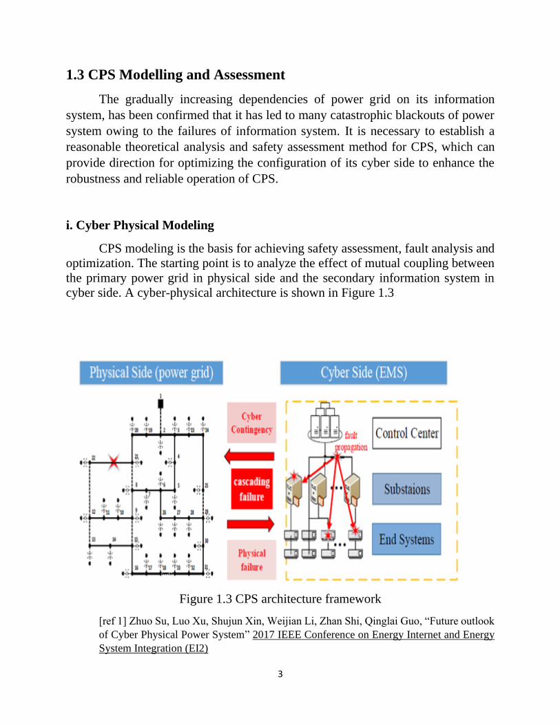
cyber side. A cyber-physical architecture is shown in Figure 1.3

Figure 1.3 CPS architecture framework

[ref 1] Zhuo Su, Luo Xu, Shujun Xin, Weijian Li, Zhan Shi, Qinglai Guo, “Future outlook

of Cyber Physical Power System” 2017 IEEE Conference on Energy Internet and Energy

System Integration (EI2)

4

The biggest challenge for cyber-physical modeling is to combine the continuous

power system based on power flow and the discrete information system. The CPS

architecture framework in figure 1.3 shows the mapping from Physical Side to Cyber

Side. The Physical Side maps to Cyber Side for physical failure. The Cyber Side

maps to Physical Side for cyber contingency. One contingency may leads to

cascading events that could trigger widespread outages.

ii. Cyber Physical Assessment

The strong interdependence of the cyber side and the physical side in power

systems, makes it very important to realize the safety analysis and reliability

assessment of CPS. The traditional approach to safety assessment usually only takes

into account the operating conditions and reliability of the primary system. However,

now the power system is more dependent on the secondary information system

measurement, sensing and control, information systems and power systems are

highly coupled. Therefore, it’s critical to realize the assessment of power systems

from CPS perspective.

1.4 Future outlook of the CPS

The current CPS modeling and simulation models are complex and not

unified. The CPS model and assessment approach based on interdependent network

theory mainly focuses on the topology analysis and lacks the quantitative calculation

of power flow. The research of information attack is often focused on a certain

situation, lack of versatility. With the further popularization of information

technology, the concept of cloud EMS, distributed EMS and IEMS is presented.

Privacy protection has received more and more attention. Privacy protection can be

regarded as a kind of cyber security issues, focusing on the confidentiality of

information in the transmission and decision process. With the implement of more

diversified, more complex and more open EMS, such as IEMS and distributed EMS,

it is necessary to establish unify CPS model and assessment approach for CPS, and

proper information masking algorithm is critical for data protection of these

information systems. The future outlook for cyber-physical power system is shown

in Figure 1.4.

5

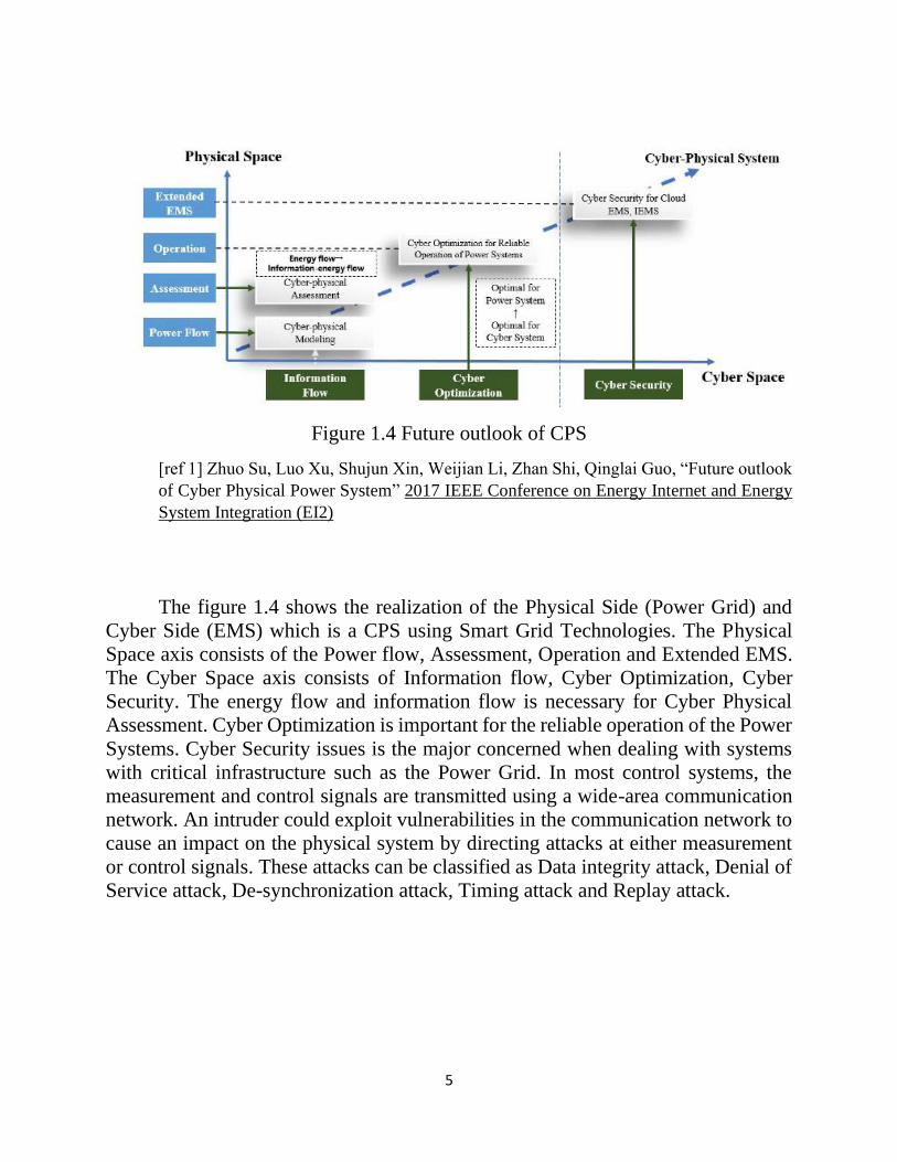
Figure 1.4 Future outlook of CPS

[ref 1] Zhuo Su, Luo Xu, Shujun Xin, Weijian Li, Zhan Shi, Qinglai Guo, “Future outlook

of Cyber Physical Power System” 2017 IEEE Conference on Energy Internet and Energy

System Integration (EI2)

The figure 1.4 shows the realization of the Physical Side (Power Grid) and

Cyber Side (EMS) which is a CPS using Smart Grid Technologies. The Physical

Space axis consists of the Power flow, Assessment, Operation and Extended EMS.

The Cyber Space axis consists of Information flow, Cyber Optimization, Cyber

Security. The energy flow and information flow is necessary for Cyber Physical

Assessment. Cyber Optimization is important for the reliable operation of the Power

Systems. Cyber Security issues is the major concerned when dealing with systems

with critical infrastructure such as the Power Grid. In most control systems, the

measurement and control signals are transmitted using a wide-area communication

network. An intruder could exploit vulnerabilities in the communication network to

cause an impact on the physical system by directing attacks at either measurement

or control signals. These attacks can be classified as Data integrity attack, Denial of

Service attack, De-synchronization attack, Timing attack and Replay attack.

6

1.5 Attack Resilient Control

State estimation has been the traditional technique for bad data detection in

power systems. As the attackers become more sophisticated and as more resources

are available to them, legacy attack detection techniques might not be sufficient. To

detect attacks of these type, advanced cyber defense techniques that incorporate

power system concepts have to be developed. Attack resilient control algorithms

provide defense in depth to the control system by adding security at the application

layer. The defense algorithms should be developed with the assumption that the

attacker has knowledge of system operation. As a basic test, the algorithm should

perform a range check to see if the obtained measurements lie within acceptable

values. Additional tests that are based on forecasts, historical data and engineering

sense should also be devised to ascertain the current state of the system. These

parameters play a part in determining the state of the system and system response to

an event. Hence, algorithms that incorporate such checks could help in identifying

malicious data when an attacker attempts to infiltrate and mislead the operator into

executing incorrect commands. Intelligent power system control algorithms that are

able to keep the system within stability limits during contingencies are critical. Also,

the development of enhanced power management systems capable of addressing

high-impact contingency scenarios.

7

Chapter 2

Power System Network Modelling

2.1 System under Study

In this section, a practical distribution network of the Taiwan Power Company

(TPC) is used as a model for restoration problem. The system is shown in figure 2.1.

It is a three phase, 11.4-kv system with 2 substations. The system consists of 11

feeders, 83 normally closed switches, and 13 normally open tie switches. Three

phase balance and constant load are assumed. Details of data are shown in table 1.

The figure 2.1 shown is modelled in ETAP 16.0.0 software and the simulations are

performed.

Fig 2.1: Distribution Network of System under study [ref. 3] Ching-Tzong Su, and Chu-Sheng Lee, “Network Reconfiguration of Distribution

Systems Using Improved Mixed-Integer Hybrid Differential Evolution”.

8

2.2 Physical Layer Modelling in ETAP 16.0.0

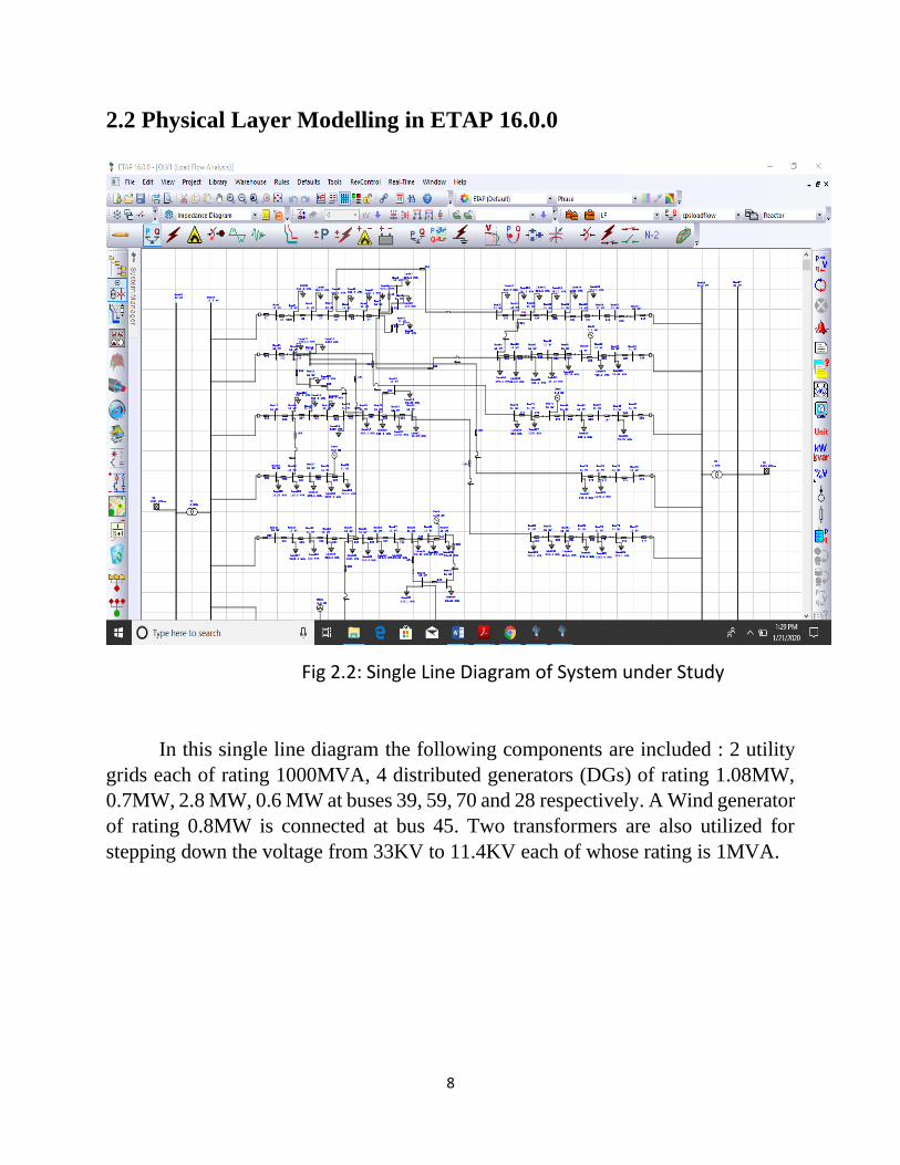
Fig 2.2: Single Line Diagram of System under Study

In this single line diagram the following components are included : 2 utility

grids each of rating 1000MVA, 4 distributed generators (DGs) of rating 1.08MW,

0.7MW, 2.8 MW, 0.6 MW at buses 39, 59, 70 and 28 respectively. A Wind generator

of rating 0.8MW is connected at bus 45. Two transformers are also utilized for

stepping down the voltage from 33KV to 11.4KV each of whose rating is 1MVA.

9

Impedance Input Data

ID R X Y Unit

Impedance Positive Sequence

Impedance

Z1 Ohm 0.1944 0.6624 0

Ohm Z3 0.2358 0.4842 0

Ohm Z4 0.0917 0.1883 0

Ohm Z5 0.2096 0.4304 0

Ohm Z6 0.0393 0.0807 0

Ohm Z7 0.0405 1380 0

Ohm Z8 0.1048 2152 0

Ohm Z9 0.2358 0.4842 0

Ohm Z10 0.1048 0.2152 0

Ohm Z11 0.0786 0.1614 0

Ohm Z12 0.3406 0.6944 0

Ohm Z13 0.0262 0.0538 0

Ohm Z14 0.0786 0.1614 0

Ohm Z15 0.1134 0.3864 0

Ohm Z16 0.0524 0.1076 0

Ohm Z17 0.0524 0.1076 0

Ohm Z18 0.1572 0.3228 0

Ohm Z19 0.0393 0.0807 0

Ohm Z20 0.1703 0.3497 0

Ohm Z21 0.2358 0.4842 0

Ohm Z22 0.1572 0.3228 0

Ohm Z23 0.1965 0.4035 0

Ohm Z24 0.131 0.269 0

Ohm Z25 0.0567 0.1932 0

Ohm Z26 0.1048 0.2152 0

Ohm Z27 0.2489 0.5111 0

Ohm Z28 0.0486 0.1656 0

Ohm Z29 0.131 0.269 0

Ohm Z30 0.1965 0.396 0

Ohm Z31 0.131 0.269 0

Ohm Z32 0.131 0.269 0

Ohm Z33 0.0262 0.0538 0

Ohm Z34 0.1703 0.3497 0

Ohm Z35 0.0524 0.1076 0

Ohm Z36 0.4978 1.0222 0

Ohm Z37 0.0393 0.0807 0

Ohm Z38 0.0393 0.0807 0

Ohm Z39 0.0786 0.1614 0

Ohm Z40 0.2096 0.4304 0

Ohm Z41 0.1965 0.4035 0

Ohm Z42 0.2096 0.4304 0

Ohm Z43 0.0486 0.1656 0

Ohm Z44 0.0393 0.0807 0

Ohm Z45 0.131 0.269 0

Ohm Z46 0.2358 0.4842 0

Ohm Z47 0.243 0.828 0

Ohm Z48 0.0655 0.1345 0

Ohm Z49 0.0655 0.1345 0

Ohm Z50 0.0393 0.0807 0

Ohm Z51 0.0786 0.1614 0

10

Table 2.1: Impedance Data of the lines/branches

Impedance Input Data

ID R X Y Unit

Impedance Positive Sequence

Impedance

Z52 Ohm 0.0393 0.0807 0

Ohm Z53 0.0786 0.1614 0

Ohm Z54 0.0524 0.1076 0

Ohm Z55 0.131 0.269 0

Ohm Z56 0.2268 0.7728 0

Ohm Z57 0.5371 1.1029 0

Ohm Z58 0.0524 0.1076 0

Ohm Z59 0.0405 0.138 0

Ohm Z60 0.0393 0.0807 0

Ohm Z61 0.0262 0.0538 0

Ohm Z62 0.1048 0.2152 0

Ohm Z63 0.2358 0.4842 0

Ohm Z64 0.0243 0.0828 0

Ohm Z65 0.0486 0.1656 0

Ohm Z66 0.1703 0.3497 0

Ohm Z67 0.1215 0.414 0

Ohm Z68 0.2187 0.7452 0

Ohm Z69 0.0486 0.1656 0

Ohm Z70 0.0729 0.2484 0

Ohm Z71 0.0567 0.1932 0

Ohm Z72 0.0262 0.0528 0

Ohm Z73 0.324 1.104 0

Ohm Z74 0.0324 0.1104 0

Ohm Z75 0.0567 0.1932 0

Ohm Z76 0.0486 0.1656 0

Ohm Z77 0.2511 0.8556 0

Ohm Z78 0.1296 0.4416 0

Ohm Z79 0.0486 0.1656 0

Ohm Z80 0.131 0.264 0

Ohm Z81 0.131 0.264 0

Ohm Z82 0.0917 0.1883 0

Ohm Z83 0.3144 0.6456 0

Ohm Z84 0.131 0.269 0

11

Bus Loading Summary Report

ID

Bus

Directly Connected Load

%PF Amp Rated Amp Loadin

g

Constant kVA Constant Z Constant I Percent

Generic

Total Bus Load

kV MW Mvar MW Mvar MW Mvar Mvar MW MVA

Bus1 11.000

Bus2 3.5 89.4 11.000 0.018 0.040

Bus3 14.8 84.8 11.000 0.072 0.169

Bus4 28.3 83.2 11.000 0.090 0.324

Bus5 80.4 81.3 11.000 0.036 0.921

Bus6 44.6 78.1 11.000 0.289 0.510

Bus7 2.8 82.7 11.000 - 0.002

Bus8 0.4 83.2 11.000 - 0.000

Bus9 0.9 79.4 11.000 - 0.001

Bus10 0.9 75.6 11.000 0.001 0.001

Bus11 100.9 81.2 11.000 1.141

Bus12 100.9 81.8 11.000 0.271 1.120

Bus13 30.6 80.0 11.000 0.203 0.339

Bus14 26.3 81.4 11.000 0.169 0.291

Bus15 133.8 80.2 11.000 1.501

Bus16 133.8 80.3 11.000 0.052 1.496

Bus17 123.6 79.6 11.000 0.120 1.377

Bus18 104.9 79.4 11.000 0.134 1.158

Bus19 80.7 76.9 11.000 0.334 0.889

Bus20 33.3 77.1 11.000 0.100 0.365

Bus21 20.5 80.9 11.000 0.116 0.225

Bus22 1.6 92.9 11.000 0.007 0.018

Bus23 3.1 95.8 11.000 0.007 0.034

Bus24 1.5 98.1 11.000 0.003 0.017

Bus25 84.2 81.3 11.000 0.011 0.953

Bus26 82.4 81.3 11.000 0.021 0.928

Bus27 78.8 81.4 11.000 0.024 0.878

Bus28 75.1 81.5 11.000 0.442 0.834

Bus29 7.1 85.8 11.000 0.041 0.079

Bus30 136.8 77.9 11.000 1.531

Bus31 136.8 78.2 11.000 0.541 1.516

Bus32 63.6 82.0 11.000 0.050 0.701

Bus33 56.0 82.3 11.000 0.033 0.617

Bus34 49.3 81.3 11.000 0.199 0.540

Bus35 19.1 83.3 11.000 0.020 0.209

Bus36 15.6 82.9 11.000 0.020 0.170

Bus37 12.1 82.0 11.000 0.003 0.132

Bus38 11.4 81.5 11.000 0.003 0.125

Bus39 1.3 89.4 11.000 0.003 0.015

Bus40 0.7 89.4 11.000 0.003 0.007

Bus41 9.4 79.6 11.000 0.052 0.103

Bus42 1.8 85.8 11.000 0.010 0.019

Bus43 81.0 47.6 11.000 0.917

Bus44 81.5 48.6 11.000 0.007 0.921

Bus45 100.0 71.0 11.000 0.245 1.126

Bus46 7.8 80.0 11.000 0.052 0.087

Bus47 184.4 81.3 11.000 2.210

Bus48 184.4 81.5 11.000 2.196

Bus49 184.4 81.7 11.000 2.183

Bus50 184.4 81.8 11.000 0.061 2.175

Bus51 176.1 82.2 11.000 0.227 2.062

12

Table 2.2: Bus Loading Data summary

ID

Bus

Directly Connected Load

%

PF

Amp Rated Amp Loadin

g

Constant kVA Constant Z Constant I Percent

Generic

Total Bus Load

kV MW Mvar MW Mvar MW Mvar Mvar MW MVA

Bus52 143.8 82.8 11.000 0.113 1.680

Bus53 125.1 82.5 11.000 0.130 1.454

Bus54 105.6 82.7 11.000 0.111 1.223

Bus55 87.0 82.2 11.000 0.029 1.002

Bus56 59.3 81.2 11.000 0.727

Bus57 59.3 81.7 11.000 0.008 0.715

Bus58 58.1 81.8 11.000 0.168 0.700

Bus59 33.8 81.7 11.000 0.407

Bus60 33.8 81.7 11.000 0.004 0.407

Bus61 33.1 81.5 11.000 0.004 0.398

Bus62 32.4 81.4 11.000 0.052 0.388

Bus63 24.5 80.6 11.000 0.095 0.293

Bus64 11.9 83.2 11.000 0.079 0.142

Bus65 108.5 77.4 11.000 1.337

Bus66 108.5 77.7 11.000 0.012 1.324

Bus67 106.6 77.9 11.000 1.288

Bus68 106.6 78.7 11.000 0.140 1.267

Bus69 89.0 79.6 11.000 1.055

Bus70 89.0 79.8 11.000 1.050

Bus71 89.0 80.0 11.000 0.570 1.046

Bus72 8.1 80.0 11.000 0.057 0.095

Bus73 62.8 79.7 11.000 0.765

Bus74 62.8 79.8 11.000 0.764

Bus75 62.8 79.9 11.000 0.386 0.762

Bus76 11.7 85.8 11.000 0.073 0.142

Bus77 143.7 80.8 11.000 1.733

Bus78 143.7 81.4 11.000 0.140 1.710

Bus79 126.2 82.5 11.000 0.503 1.495

Bus80 48.4 80.2 11.000 0.054 0.572

Bus81 40.5 80.0 11.000 0.138 0.477

Bus82 20.5 78.8 11.000 0.011 0.241

Bus83 17.4 74.3 11.000 0.136 0.204

Bus84 502.0 72.2 11.400 5.699

Bus85 164.1 51.4 33.000 9.522

Bus86 558.7 79.3 11.400 6.907

Bus87 193.0 60.9 33.000 11.198

13

Chapter 3

Physical Layer Simulation in ETAP 16.0.0

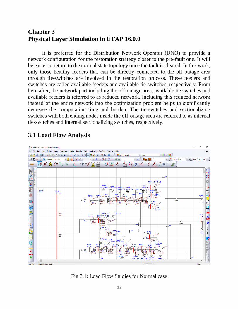
It is preferred for the Distribution Network Operator (DNO) to provide a

network configuration for the restoration strategy closer to the pre-fault one. It will

be easier to return to the normal state topology once the fault is cleared. In this work,

only those healthy feeders that can be directly connected to the off-outage area

through tie-switches are involved in the restoration process. These feeders and

switches are called available feeders and available tie-switches, respectively. From

here after, the network part including the off-outage area, available tie switches and

available feeders is referred to as reduced network. Including this reduced network

instead of the entire network into the optimization problem helps to significantly

decrease the computation time and burden. The tie-switches and sectionalizing

switches with both ending nodes inside the off-outage area are referred to as internal

tie-switches and internal sectionalizing switches, respectively.

3.1 Load Flow Analysis

Fig 3.1: Load Flow Studies for Normal case

14

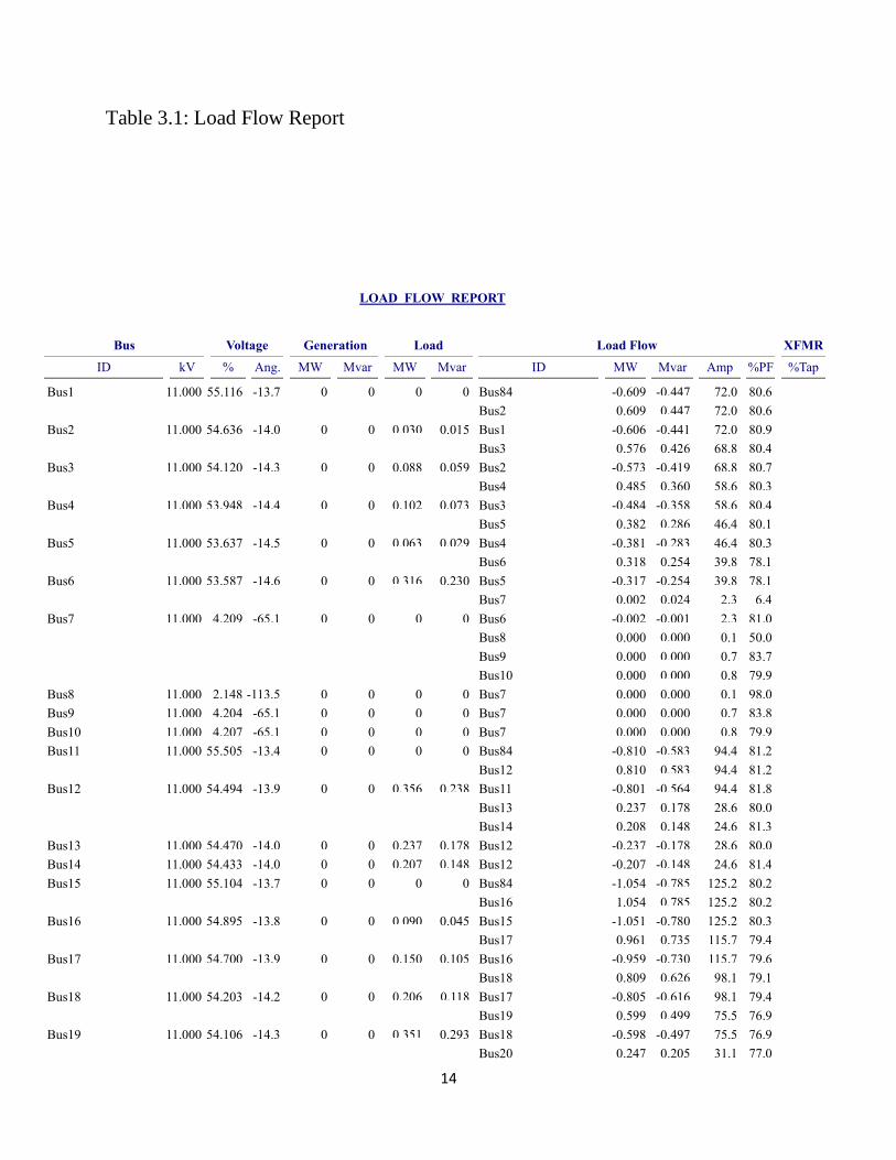
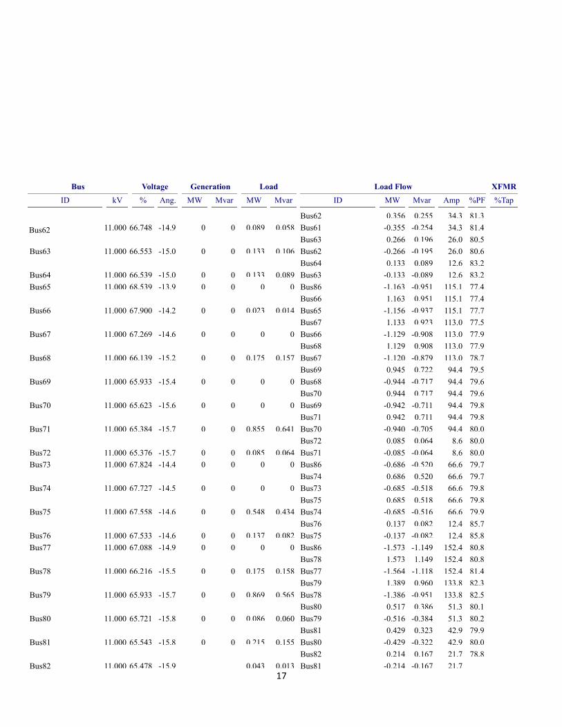
Table 3.1: Load Flow Report

LOAD FLOW REPORT

Bus

ID kV

Voltage

Ang. %

Mag.

Generation

MW Mvar

Load

MW Mvar

Load Flow

MW Mvar Amp ID %PF

XFMR

%Tap

Bus1 11.000 -13.7 55.116 Bus84 -0.609 -0.447 72.0 80.6 0 0 0 0

Bus2 0.609 0.447 72.0 80.6

Bus2 11.000 -14.0 54.636 0.015 0.030 Bus1 -0.606 -0.441 72.0 80.9 0 0

Bus3 0.576 0.426 68.8 80.4

Bus3 11.000 -14.3 54.120 0.059 0.088 Bus2 -0.573 -0.419 68.8 80.7 0 0

Bus4 0.485 0.360 58.6 80.3

Bus4 11.000 -14.4 53.948 0.073 0.102 Bus3 -0.484 -0.358 58.6 80.4 0 0

Bus5 0.382 0.286 46.4 80.1

Bus5 11.000 -14.5 53.637 0.029 0.063 Bus4 -0.381 -0.283 46.4 80.3 0 0

Bus6 0.318 0.254 39.8 78.1

Bus6 11.000 -14.6 53.587 0.230 0.316 Bus5 -0.317 -0.254 39.8 78.1 0 0

Bus7 0.002 0.024 2.3 6.4

Bus7 11.000 -65.1 4.209 Bus6 -0.002 -0.001 2.3 81.0 0 0 0 0

Bus8 0.000 0.000 0.1 50.0

Bus9 0.000 0.000 0.7 83.7

Bus10 0.000 0.000 0.8 79.9

Bus8 11.000 -113.5 2.148 Bus7 0.000 0.000 0.1 98.0 0 0 0 0

Bus9 11.000 -65.1 4.204 Bus7 0.000 0.000 0.7 83.8 0 0 0 0

Bus10 11.000 -65.1 4.207 Bus7 0.000 0.000 0.8 79.9 0 0 0 0

Bus11 11.000 -13.4 55.505 Bus84 -0.810 -0.583 94.4 81.2 0 0 0 0

Bus12 0.810 0.583 94.4 81.2

Bus12 11.000 -13.9 54.494 0.238 0.356 Bus11 -0.801 -0.564 94.4 81.8 0 0

Bus13 0.237 0.178 28.6 80.0

Bus14 0.208 0.148 24.6 81.3

Bus13 11.000 -14.0 54.470 0.178 0.237 Bus12 -0.237 -0.178 28.6 80.0 0 0

Bus14 11.000 -14.0 54.433 0.148 0.207 Bus12 -0.207 -0.148 24.6 81.4 0 0

Bus15 11.000 -13.7 55.104 Bus84 -1.054 -0.785 125.2 80.2 0 0 0 0

Bus16 1.054 0.785 125.2 80.2

Bus16 11.000 -13.8 54.895 0.045 0.090 Bus15 -1.051 -0.780 125.2 80.3 0 0

Bus17 0.961 0.735 115.7 79.4

Bus17 11.000 -13.9 54.700 0.105 0.150 Bus16 -0.959 -0.730 115.7 79.6 0 0

Bus18 0.809 0.626 98.1 79.1

Bus18 11.000 -14.2 54.203 0.118 0.206 Bus17 -0.805 -0.616 98.1 79.4 0 0

Bus19 0.599 0.499 75.5 76.9

Bus19 11.000 -14.3 54.106 0.293 0.351 Bus18 -0.598 -0.497 75.5 76.9 0 0

Bus20 0.247 0.205 31.1 77.0

15

Bus

ID kV

Voltage

Ang. %

Mag.

Generation

MW Mvar

Load

MW Mvar

Load Flow

MW Mvar Amp ID %PF

XFMR

%Tap

Bus20 11.000 -14.3 53.932 0.087 0.087 Bus19 -0.247 -0.204 31.1 77.1 0 0

Bus21 0.159 0.116 19.2 80.8

Bus21 11.000 -14.4 53.789 0.101 0.116 Bus20 -0.159 -0.116 19.2 80.9 0 0

Bus22 0.014 0.006 1.5 92.8

Bus23 0.029 0.009 2.9 95.8

Bus22 11.000 -14.4 53.782 0.006 0.014 Bus21 -0.014 -0.006 1.5 92.9 0 0

Bus23 11.000 -14.4 53.774 0.006 0.014 Bus21 -0.029 -0.009 2.9 95.8 0 0

Bus24 0.014 0.003 1.4 98.1

Bus24 11.000 -14.4 53.770 0.003 0.014 Bus23 -0.014 -0.003 1.4 98.1 0 0

Bus25 11.000 -13.4 55.543 0.009 0.015 Bus84 -0.678 -0.486 78.8 81.3 0 0

Bus26 0.662 0.477 77.1 81.2

Bus26 11.000 -13.5 55.287 0.018 0.031 Bus25 -0.661 -0.473 77.1 81.3 0 0

Bus27 0.630 0.454 73.7 81.1

Bus27 11.000 -13.9 54.707 0.021 0.030 Bus26 -0.626 -0.446 73.7 81.4 0 0

Bus28 0.596 0.425 70.2 81.4

Bus28 11.000 -14.0 54.557 0.387 0.536 Bus27 -0.595 -0.423 70.2 81.5 0 0

Bus29 0.059 0.036 6.7 85.7

Bus29 11.000 -14.0 54.530 0.036 0.059 Bus28 -0.059 -0.036 6.7 85.8 0 0

Bus30 11.000 -13.6 54.929 Bus84 -1.043 -0.841 128.0 77.9 0 0 0 0

Bus31 1.043 0.841 128.0 77.9

Bus31 11.000 -13.9 54.384 0.473 0.532 Bus30 -1.037 -0.827 128.0 78.2 0 0

Bus32 0.504 0.354 59.5 81.8

Bus32 11.000 -14.0 54.139 0.044 0.059 Bus31 -0.503 -0.351 59.5 82.0 0 0

Bus33 0.444 0.307 52.4 82.3

Bus33 11.000 -14.1 54.096 0.029 0.059 Bus32 -0.444 -0.307 52.4 82.3 0 0

Bus34 0.386 0.278 46.1 81.2

Bus34 11.000 -14.2 53.848 0.174 0.232 Bus33 -0.385 -0.275 46.1 81.3 0 0

Bus35 0.153 0.101 17.9 83.3

Bus35 11.000 -14.2 53.819 0.017 0.029 Bus34 -0.153 -0.101 17.9 83.3 0 0

Bus36 0.124 0.084 14.6 82.7

Bus36 11.000 -14.4 53.593 0.017 0.029 Bus35 -0.123 -0.083 14.6 82.9 0 0

Bus37 0.095 0.066 11.3 82.0

Bus37 11.000 -14.4 53.579 0.003 0.006 Bus36 -0.095 -0.066 11.3 82.0 0 0

Bus38 0.089 0.063 10.7 81.5

Bus38 11.000 -14.4 53.565 0.003 0.006 Bus37 -0.089 -0.063 10.7 81.5 0 0

Bus39 0.011 0.006 1.3 89.4

Bus41 0.072 0.054 8.8 79.6

Bus39 11.000 -14.4 53.563 0.003 0.006 Bus38 -0.011 -0.006 1.3 89.4 0 0

Bus40 0.006 0.003 0.6 89.4

Bus

ID kV

Voltage

Ang. %

Mag.

Generation

MW Mvar

Load

MW Mvar

Load Flow

MW Mvar Amp ID %PF

XFMR

%Tap

Bus40 11.000 -14.4 53.559 0.003 0.006 Bus39 -0.006 -0.003 0.6 89.4 0 0

Bus41 11.000 -14.4 53.510 0.046 0.057 Bus38 -0.072 -0.054 8.8 79.6 0 0

Bus42 0.014 0.009 1.6 85.7

Bus42 11.000 -14.4 53.500 0.009 0.014 Bus41 -0.014 -0.009 1.6 85.8 0

16

0

Bus43 11.000 -13.1 55.585 Bus84 0.481 -0.770 85.7 -53.0 0 0 0 0

Bus44 -0.481 0.770 85.7 -53.0

Bus44 11.000 -13.0 55.521 0.006 0.009 Bus43 0.482 -0.768 85.7 -53.2 0 0

Bus45 -0.491 0.762 85.7 -54.2

Bus45 11.000 -12.6 55.313 -0.496 0.800 0.214 0.245 Bus44 0.494 -0.756 85.7 -54.7

Bus46 0.061 0.046 7.3 80.0

Bus46 11.000 -12.6 55.258 0.046 0.061 Bus45 -0.061 -0.046 7.3 80.0 0 0

Bus47 11.000 -14.6 67.604 Bus86 -1.210 -0.817 113.3 82.9 0 0 0 0

Bus48 1.210 0.817 113.3 82.9

Bus48 11.000 -14.7 67.373 Bus47 -1.207 -0.812 113.3 83.0 0 0 0 0

Bus49 1.207 0.812 113.3 83.0

Bus49 11.000 -14.8 67.143 Bus48 -1.205 -0.807 113.3 83.1 0 0 0 0

Bus50 1.205 0.807 113.3 83.1

Bus50 11.000 -14.9 67.004 0.072 0.090 Bus49 -1.203 -0.803 113.3 83.2 0 0

Bus51 1.114 0.732 104.4 83.6

Bus51 11.000 -15.0 66.751 0.267 0.356 Bus50 -1.111 -0.726 104.4 83.7 0 0

Bus52 0.755 0.459 69.4 85.4

Bus52 11.000 -15.1 66.668 0.133 0.222 Bus51 -0.754 -0.458 69.4 85.5 0 0

Bus53 0.532 0.325 49.0 85.4

Bus53 11.000 -15.2 66.551 0.155 0.221 Bus52 -0.531 -0.323 49.0 85.4 0 0

Bus54 0.310 0.168 27.8 87.9

Bus54 11.000 -15.2 66.509 0.133 0.221 Bus53 -0.310 -0.168 27.8 87.9 0 0

Bus55 0.088 0.035 7.5 92.8

Bus55 11.000 -15.2 66.483 0.035 0.088 Bus54 -0.088 -0.035 7.5 92.9 0 0

Bus56 11.000 -14.2 68.167 Bus86 -0.664 -0.476 62.9 81.2 0 0 0 0

Bus57 0.664 0.476 62.9 81.2

Bus57 11.000 -14.7 67.100 0.009 0.014 Bus56 -0.657 -0.463 62.9 81.7 0 0

Bus58 0.644 0.454 61.6 81.7

Bus58 11.000 -14.7 66.999 0.189 0.269 Bus57 -0.643 -0.453 61.6 81.8 0 0

Bus59 0.374 0.265 35.9 81.6

Bus59 11.000 -14.8 66.935 Bus58 -0.374 -0.264 35.9 81.7 0 0 0 0

Bus60 0.374 0.264 35.9 81.7

Bus60 11.000 -14.8 66.890 0.004 0.009 Bus59 -0.374 -0.264 35.9 81.7 0 0

Bus61 0.365 0.259 35.1 81.5

Bus61 11.000 -14.8 66.861 0.004 0.009 Bus60 -0.365 -0.259 35.1 81.5 0 0

Bus

ID kV

Voltage

Ang. %

Mag.

Generation

MW Mvar

Load

MW Mvar

Load Flow

MW Mvar Amp ID %PF

XFMR

%Tap

Bus40 11.000 -14.4 53.559 0.003 0.006 Bus39 -0.006 -0.003 0.6 89.4 0 0

Bus41 11.000 -14.4 53.510 0.046 0.057 Bus38 -0.072 -0.054 8.8 79.6 0 0

Bus42 0.014 0.009 1.6 85.7

Bus42 11.000 -14.4 53.500 0.009 0.014 Bus41 -0.014 -0.009 1.6 85.8 0 0

Bus43 11.000 -13.1 55.585 Bus84 0.481 -0.770 85.7 -53.0 0 0 0 0

Bus44 -0.481 0.770 85.7 -53.0

Bus44 11.000 -13.0 55.521 0.006 0.009 Bus43 0.482 -0.768 85.7 -53.2 0 0

Bus45 -0.491 0.762 85.7 -54.2

Bus45 11.000 -12.6 55.313 -0.496 0.800 0.214 0.245 Bus44 0.494 -0.756 85.7 -54.7

Bus46 0.061 0.046 7.3 80.0

Bus46 11.000 -12.6 55.258 0.046 0.061 Bus45 -0.061 -0.046 7.3 80.0 0 0

Bus47 11.000 -14.6 67.604 Bus86 -1.210 -0.817 113.3 82.9 0 0 0 0

Bus48 1.210 0.817 113.3 82.9

Bus48 11.000 -14.7 67.373 Bus47 -1.207 -0.812 113.3 83.0 0 0 0 0

Bus49 1.207 0.812 113.3 83.0

Bus49 11.000 -14.8 67.143 Bus48 -1.205 -0.807 113.3 83.1 0 0 0 0

Bus50 1.205 0.807 113.3 83.1

Bus50 11.000 -14.9 67.004 0.072 0.090 Bus49 -1.203 -0.803 113.3 83.2 0 0

Bus51 1.114 0.732 104.4 83.6

Bus51 11.000 -15.0 66.751 0.267 0.356 Bus50 -1.111 -0.726 104.4 83.7 0 0

Bus52 0.755 0.459 69.4 85.4

Bus52 11.000 -15.1 66.668 0.133 0.222 Bus51 -0.754 -0.458 69.4 85.5 0 0

Bus53 0.532 0.325 49.0 85.4

Bus53 11.000 -15.2 66.551 0.155 0.221 Bus52 -0.531 -0.323 49.0 85.4 0 0

Bus54 0.310 0.168 27.8 87.9

Bus54 11.000 -15.2 66.509 0.133 0.221 Bus53 -0.310 -0.168 27.8 87.9 0 0

Bus55 0.088 0.035 7.5 92.8

Bus55 11.000 -15.2 66.483 0.035 0.088 Bus54 -0.088 -0.035 7.5 92.9 0 0

Bus56 11.000 -14.2 68.167 Bus86 -0.664 -0.476 62.9 81.2 0 0 0 0

Bus57 0.664 0.476 62.9 81.2

Bus57 11.000 -14.7 67.100 0.009 0.014 Bus56 -0.657 -0.463 62.9 81.7 0 0

Bus58 0.644 0.454 61.6 81.7

Bus58 11.000 -14.7 66.999 0.189 0.269 Bus57 -0.643 -0.453 61.6 81.8 0 0

Bus59 0.374 0.265 35.9 81.6

Bus59 11.000 -14.8 66.935 Bus58 -0.374 -0.264 35.9 81.7 0 0 0 0

Bus60 0.374 0.264 35.9 81.7

Bus60 11.000 -14.8 66.890 0.004 0.009 Bus59 -0.374 -0.264 35.9 81.7 0 0

Bus61 0.365 0.259 35.1 81.5

Bus61 11.000 -14.8 66.861 0.004 0.009 Bus60 -0.365 -0.259 35.1

17

Bus

ID kV

Voltage

Ang. %

Mag.

Generation

MW Mvar

Load

MW Mvar

Load Flow

MW Mvar Amp ID %PF

XFMR

%Tap

Bus62 0.356 0.255 34.3 81.3

Bus62 11.000 -14.9 66.748 0.058 0.089 Bus61 -0.355 -0.254 34.3 81.4 0 0

Bus63 0.266 0.196 26.0 80.5

Bus63 11.000 -15.0 66.553 0.106 0.133 Bus62 -0.266 -0.195 26.0 80.6 0 0

Bus64 0.133 0.089 12.6 83.2

Bus64 11.000 -15.0 66.539 0.089 0.133 Bus63 -0.133 -0.089 12.6 83.2 0 0

Bus65 11.000 -13.9 68.539 Bus86 -1.163 -0.951 115.1 77.4 0 0 0 0

Bus66 1.163 0.951 115.1 77.4

Bus66 11.000 -14.2 67.900 0.014 0.023 Bus65 -1.156 -0.937 115.1 77.7 0 0

Bus67 1.133 0.923 113.0 77.5

Bus67 11.000 -14.6 67.269 Bus66 -1.129 -0.908 113.0 77.9 0 0 0 0

Bus68 1.129 0.908 113.0 77.9

Bus68 11.000 -15.2 66.139 0.157 0.175 Bus67 -1.120 -0.879 113.0 78.7 0 0

Bus69 0.945 0.722 94.4 79.5

Bus69 11.000 -15.4 65.933 Bus68 -0.944 -0.717 94.4 79.6 0 0 0 0

Bus70 0.944 0.717 94.4 79.6

Bus70 11.000 -15.6 65.623 Bus69 -0.942 -0.711 94.4 79.8 0 0 0 0

Bus71 0.942 0.711 94.4 79.8

Bus71 11.000 -15.7 65.384 0.641 0.855 Bus70 -0.940 -0.705 94.4 80.0 0 0

Bus72 0.085 0.064 8.6 80.0

Bus72 11.000 -15.7 65.376 0.064 0.085 Bus71 -0.085 -0.064 8.6 80.0 0 0

Bus73 11.000 -14.4 67.824 Bus86 -0.686 -0.520 66.6 79.7 0 0 0 0

Bus74 0.686 0.520 66.6 79.7

Bus74 11.000 -14.5 67.727 Bus73 -0.685 -0.518 66.6 79.8 0 0 0 0

Bus75 0.685 0.518 66.6 79.8

Bus75 11.000 -14.6 67.558 0.434 0.548 Bus74 -0.685 -0.516 66.6 79.9 0 0

Bus76 0.137 0.082 12.4 85.7

Bus76 11.000 -14.6 67.533 0.082 0.137 Bus75 -0.137 -0.082 12.4 85.8 0 0

Bus77 11.000 -14.9 67.088 Bus86 -1.573 -1.149 152.4 80.8 0 0 0 0

Bus78 1.573 1.149 152.4 80.8

Bus78 11.000 -15.5 66.216 0.158 0.175 Bus77 -1.564 -1.118 152.4 81.4 0 0

Bus79 1.389 0.960 133.8 82.3

Bus79 11.000 -15.7 65.933 0.565 0.869 Bus78 -1.386 -0.951 133.8 82.5 0 0

Bus80 0.517 0.386 51.3 80.1

Bus80 11.000 -15.8 65.721 0.060 0.086 Bus79 -0.516 -0.384 51.3 80.2 0 0

Bus81 0.429 0.323 42.9 79.9

Bus81 11.000 -15.8 65.543 0.155 0.215 Bus80 -0.429 -0.322 42.9 80.0 0 0

Bus82 0.214 0.167 21.7 78.8

Bus82 11.000 -15.9 65.478 0.013 0.043 Bus81 -0.214 -0.167 21.7

18

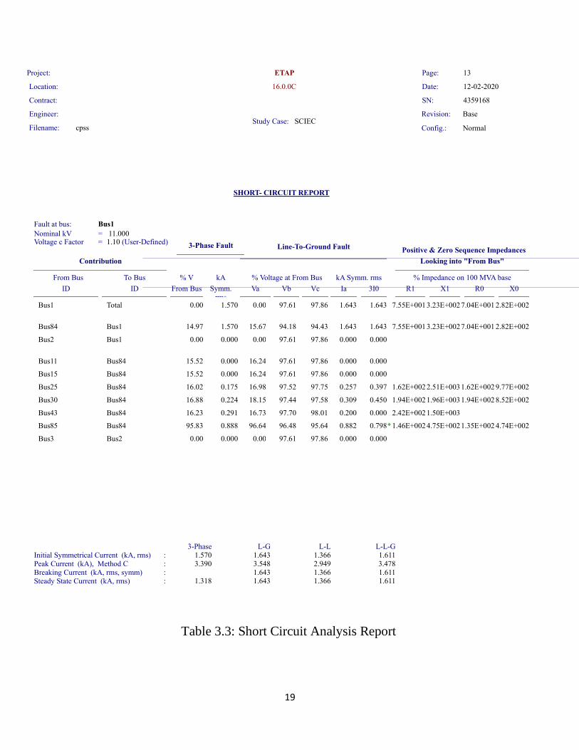
3.2 Short Circuit Analysis

Fig 3.2: Short Circuit Analysis of the System under Study (fault at bus 1)

19

Project:

Study Case: SCIEC Revision: Base

Config.: Normal

Location:

Contract:

Engineer:

Filename: cpss

ETAP

16.0.0C

Page: 13

Date: 12-02-2020

SN: 4359168

SHORT- CIRCUIT REPORT

Fault at bus:

Looking into "From Bus"

ID Symm.

rms From Bus ID Va

From Bus To Bus % V kA % Voltage at From Bus

Contribution

3-Phase Fault

Vb Vc Ia 3I0 R1 X1 R0 X0

kA Symm. rms % Impedance on 100 MVA base

Line-To-Ground Fault Positive & Zero Sequence Impedances

Nominal kV Voltage c Factor

Bus1

= 1.10 (User-Defined) = 11.000

Bus1 Total 0.00 1.570 0.00 97.61 97.86 1.643 1.643 7.04E+001 2.82E+002 7.55E+001 3.23E+002

Bus84 Bus1 14.97 1.570 15.67 94.18 94.43 1.643 1.643 7.04E+001 2.82E+002 7.55E+001 3.23E+002

Bus2 Bus1 0.00 0.000 0.00 97.61 97.86 0.000 0.000

Bus11 Bus84 15.52 0.000 16.24 97.61 97.86 0.000 0.000

Bus15 Bus84 15.52 0.000 16.24 97.61 97.86 0.000 0.000

Bus25 Bus84 16.02 0.175 16.98 97.52 97.75 0.257 0.397 1.62E+002 9.77E+002 1.62E+002 2.51E+003

Bus30 Bus84 16.88 0.224 18.15 97.44 97.58 0.309 0.450 1.94E+002 8.52E+002 1.94E+002 1.96E+003

Bus43 Bus84 16.23 0.291 16.73 97.70 98.01 0.200 0.000 2.42E+002 1.50E+003

Bus85 Bus84 95.83 0.888 96.64 96.48 95.64 0.882 0.798 1.35E+002 4.74E+002 1.46E+002 4.75E+002 *

Bus3 Bus2 0.00 0.000 0.00 97.61 97.86 0.000 0.000

Initial Symmetrical Current (kA, rms) :

3-Phase L-G L-L L-L-G

1.570 Peak Current (kA), Method C Breaking Current (kA, rms, symm) Steady State Current (kA, rms)

: : :

3.390

1.318

1.643 3.548 1.643 1.643

1.366 2.949 1.366 1.366

1.611 3.478 1.611 1.611

Table 3.3: Short Circuit Analysis Report

20

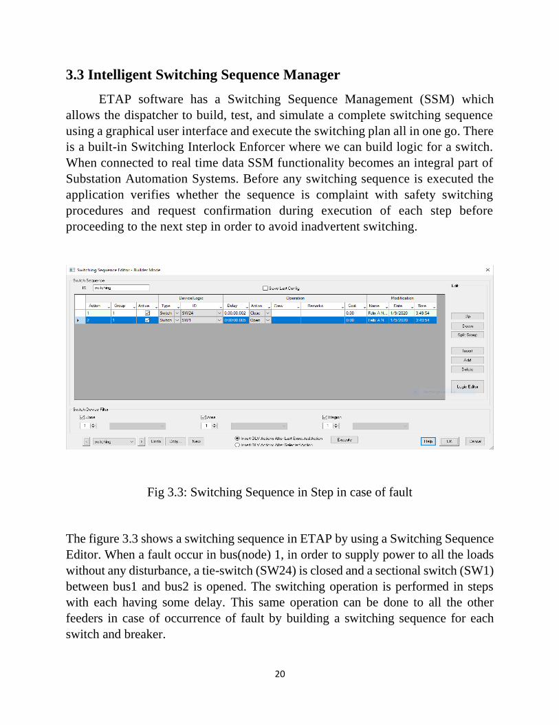
3.3 Intelligent Switching Sequence Manager

ETAP software has a Switching Sequence Management (SSM) which

allows the dispatcher to build, test, and simulate a complete switching sequence

using a graphical user interface and execute the switching plan all in one go. There

is a built-in Switching Interlock Enforcer where we can build logic for a switch.

When connected to real time data SSM functionality becomes an integral part of

Substation Automation Systems. Before any switching sequence is executed the

application verifies whether the sequence is complaint with safety switching

procedures and request confirmation during execution of each step before

proceeding to the next step in order to avoid inadvertent switching.

Fig 3.3: Switching Sequence in Step in case of fault

The figure 3.3 shows a switching sequence in ETAP by using a Switching Sequence

Editor. When a fault occur in bus(node) 1, in order to supply power to all the loads

without any disturbance, a tie-switch (SW24) is closed and a sectional switch (SW1)

between bus1 and bus2 is opened. The switching operation is performed in steps

with each having some delay. This same operation can be done to all the other

feeders in case of occurrence of fault by building a switching sequence for each

switch and breaker.

21

Chapter 4

Cyber Physical System Application

Fig 4.1: Single Line Diagram of Six Bus System under Study

22

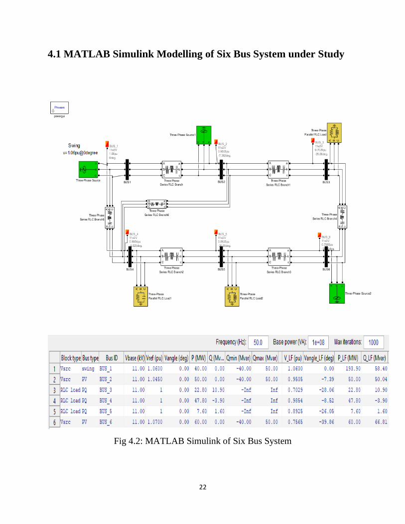
4.1 MATLAB Simulink Modelling of Six Bus System under Study

Fig 4.2: MATLAB Simulink of Six Bus System

23

Chapter 5

State Estimation Controller

The State Estimation algorithm used to build the controller for SCADA is

‘Weighted Least Square Method’. As it is difficult to realize a real PMU, in this

work the PMUs measurements data are assumed to be collected initially before

running the algorithm. The measurements data of real and reactive power are

assumed to be known and the unknown values or state vectors to be determined using

WLS algorithm are voltages and bus angles. Using State Estimation technique the

bad data injected to the buses in normal and abnormal conditions can be corrected

by comparing with the data assigned by the algorithm, and the residual values can

be discarded.

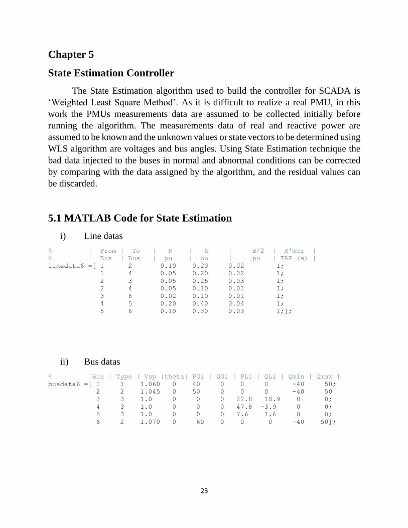
5.1 MATLAB Code for State Estimation

i) Line datas

% | From | To | R | X | B/2 | X'mer |

% | Bus | Bus | pu | pu | pu | TAP (a) |

linedata6 =[ 1 2 0.10 0.20 0.02 1;

1 4 0.05 0.20 0.02 1;

2 3 0.05 0.25 0.03 1;

2 4 0.05 0.10 0.01 1;

3 6 0.02 0.10 0.01 1;

4 5 0.20 0.40 0.04 1;

5 6 0.10 0.30 0.03 1;];

ii) Bus datas

% |Bus | Type | Vsp |theta| PGi | QGi | PLi | QLi | Qmin | Qmax |

busdata6 =[ 1 1 1.060 0 40 0 0 0 -40 50;

2 2 1.045 0 50 0 0 0 -40 50

3 3 1.0 0 0 0 22.8 10.9 0 0;

4 3 1.0 0 0 0 47.8 -3.9 0 0;

5 3 1.0 0 0 0 7.6 1.6 0 0;

6 2 1.070 0 60 0 0 0 -40 50];

24

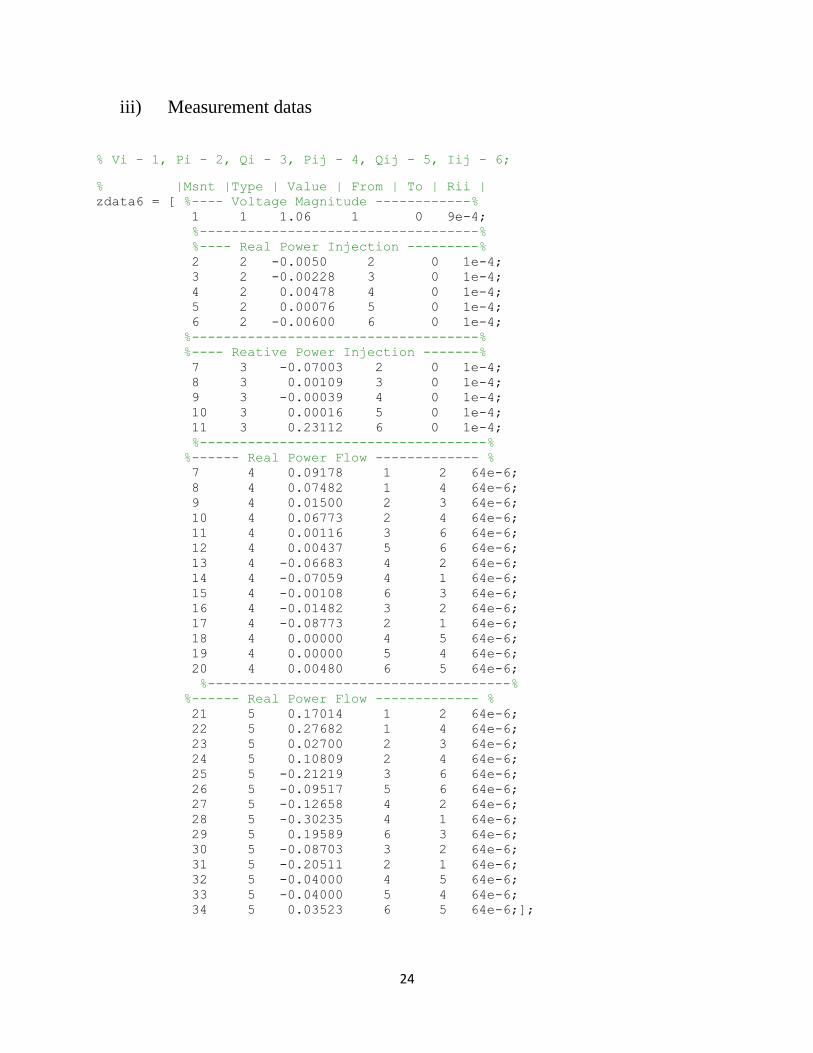
iii) Measurement datas

% Vi - 1, Pi - 2, Qi - 3, Pij - 4, Qij - 5, Iij - 6;

% |Msnt |Type | Value | From | To | Rii | zdata6 = [ %---- Voltage Magnitude ------------% 1 1 1.06 1 0 9e-4; %-----------------------------------% %---- Real Power Injection ---------% 2 2 -0.0050 2 0 1e-4; 3 2 -0.00228 3 0 1e-4; 4 2 0.00478 4 0 1e-4; 5 2 0.00076 5 0 1e-4; 6 2 -0.00600 6 0 1e-4; %------------------------------------% %---- Reative Power Injection -------% 7 3 -0.07003 2 0 1e-4; 8 3 0.00109 3 0 1e-4; 9 3 -0.00039 4 0 1e-4; 10 3 0.00016 5 0 1e-4; 11 3 0.23112 6 0 1e-4; %------------------------------------% %------ Real Power Flow ------------- % 7 4 0.09178 1 2 64e-6; 8 4 0.07482 1 4 64e-6; 9 4 0.01500 2 3 64e-6; 10 4 0.06773 2 4 64e-6; 11 4 0.00116 3 6 64e-6; 12 4 0.00437 5 6 64e-6; 13 4 -0.06683 4 2 64e-6; 14 4 -0.07059 4 1 64e-6; 15 4 -0.00108 6 3 64e-6; 16 4 -0.01482 3 2 64e-6; 17 4 -0.08773 2 1 64e-6; 18 4 0.00000 4 5 64e-6; 19 4 0.00000 5 4 64e-6; 20 4 0.00480 6 5 64e-6; %--------------------------------------% %------ Real Power Flow ------------- % 21 5 0.17014 1 2 64e-6; 22 5 0.27682 1 4 64e-6; 23 5 0.02700 2 3 64e-6; 24 5 0.10809 2 4 64e-6; 25 5 -0.21219 3 6 64e-6; 26 5 -0.09517 5 6 64e-6; 27 5 -0.12658 4 2 64e-6; 28 5 -0.30235 4 1 64e-6; 29 5 0.19589 6 3 64e-6; 30 5 -0.08703 3 2 64e-6; 31 5 -0.20511 2 1 64e-6; 32 5 -0.04000 4 5 64e-6; 33 5 -0.04000 5 4 64e-6; 34 5 0.03523 6 5 64e-6;];

25

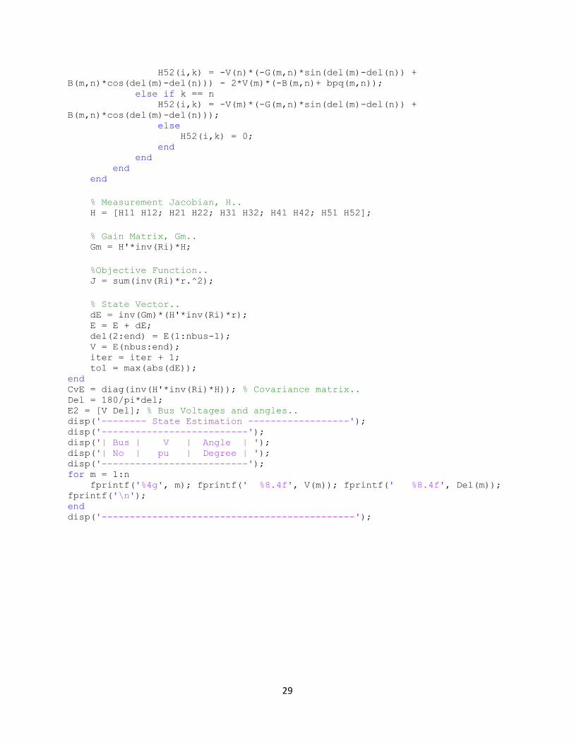
iv) Power System State Estimation using Weighted Least Square Method

num =6; % six bus system ybus = ybusppg(num); % Get YBus.. zdata = zdatas(num); % Get Measurement data.. bpq = bbusppg(num); % Get B data.. nbus = max(max(zdata(:,4)),max(zdata(:,5))); % Get number of buses.. type = zdata(:,2); % Type of measurement, Vi - 1, Pi - 2, Qi - 3, Pij - 4,

Qij - 5, Iij - 6.. z = zdata(:,3); % Measuement values.. fbus = zdata(:,4); % From bus.. tbus = zdata(:,5); % To bus.. Ri = diag(zdata(:,6)); % Measurement Error.. V = ones(nbus,1); % Initialize the bus voltages.. del = zeros(nbus,1); % Initialize the bus angles.. E = [del(2:end); V]; % State Vector.. G = real(ybus); B = imag(ybus); vi = find(type == 1); % Index of voltage magnitude measurements.. ppi = find(type == 2); % Index of real power injection measurements.. qi = find(type == 3); % Index of reactive power injection measurements.. pf = find(type == 4); % Index of real powerflow measurements.. qf = find(type == 5); % Index of reactive powerflow measurements.. nvi = length(vi); % Number of Voltage measurements.. npi = length(ppi); % Number of Real Power Injection measurements.. nqi = length(qi); % Number of Reactive Power Injection measurements.. npf = length(pf); % Number of Real Power Flow measurements.. nqf = length(qf); % Number of Reactive Power Flow measurements.. iter = 1; tol = 5; while(tol > 1e-4)

%Measurement Function, h h1 = V(fbus(vi),1); h2 = zeros(npi,1); h3 = zeros(nqi,1); h4 = zeros(npf,1); h5 = zeros(nqf,1);

for i = 1:npi m = fbus(ppi(i)); for k = 1:nbus h2(i) = h2(i) + V(m)*V(k)*(G(m,k)*cos(del(m)-del(k)) +

B(m,k)*sin(del(m)-del(k))); end end

for i = 1:nqi m = fbus(qi(i)); for k = 1:nbus h3(i) = h3(i) + V(m)*V(k)*(G(m,k)*sin(del(m)-del(k)) -

B(m,k)*cos(del(m)-del(k))); end end

26

for i = 1:npf m = fbus(pf(i)); n = tbus(pf(i)); h4(i) = -V(m)^2*G(m,n) - V(m)*V(n)*(-G(m,n)*cos(del(m)-del(n)) -

B(m,n)*sin(del(m)-del(n))); end

for i = 1:nqf m = fbus(qf(i)); n = tbus(qf(i)); h5(i) = -V(m)^2*(-B(m,n)+bpq(m,n)) - V(m)*V(n)*(-G(m,n)*sin(del(m)-

del(n)) + B(m,n)*cos(del(m)-del(n))); end

h = [h1; h2; h3; h4; h5];

% Residue.. r = z - h;

% Jacobian.. % H11 - Derivative of V with respect to angles.. All Zeros H11 = zeros(nvi,nbus-1); % H12 - Derivative of V with respect to V.. H12 = zeros(nvi,nbus); for k = 1:nvi for n = 1:nbus if n == k H12(k,n) = 1; end end end % H21 - Derivative of Real Power Injections with Angles.. H21 = zeros(npi,nbus-1); for i = 1:npi m = fbus(ppi(i)); for k = 1:(nbus-1) if k+1 == m for n = 1:nbus H21(i,k) = H21(i,k) + V(m)* V(n)*(-G(m,n)*sin(del(m)-

del(n)) + B(m,n)*cos(del(m)-del(n))); end H21(i,k) = H21(i,k) - V(m)^2*B(m,m); else H21(i,k) = V(m)* V(k+1)*(G(m,k+1)*sin(del(m)-del(k+1)) -

B(m,k+1)*cos(del(m)-del(k+1))); end end end

% H22 - Derivative of Real Power Injections with V.. H22 = zeros(npi,nbus); for i = 1:npi m = fbus(ppi(i)); for k = 1:(nbus) if k == m for n = 1:nbus

27

H22(i,k) = H22(i,k) + V(n)*(G(m,n)*cos(del(m)-del(n)) +

B(m,n)*sin(del(m)-del(n))); end H22(i,k) = H22(i,k) + V(m)*G(m,m); else H22(i,k) = V(m)*(G(m,k)*cos(del(m)-del(k)) +

B(m,k)*sin(del(m)-del(k))); end end end

% H31 - Derivative of Reactive Power Injections with Angles.. H31 = zeros(nqi,nbus-1); for i = 1:nqi m = fbus(qi(i)); for k = 1:(nbus-1) if k+1 == m for n = 1:nbus H31(i,k) = H31(i,k) + V(m)* V(n)*(G(m,n)*cos(del(m)-

del(n)) + B(m,n)*sin(del(m)-del(n))); end H31(i,k) = H31(i,k) - V(m)^2*G(m,m); else H31(i,k) = V(m)* V(k+1)*(-G(m,k+1)*cos(del(m)-del(k+1)) -

B(m,k+1)*sin(del(m)-del(k+1))); end end end

% H32 - Derivative of Reactive Power Injections with V.. H32 = zeros(nqi,nbus); for i = 1:nqi m = fbus(qi(i)); for k = 1:(nbus) if k == m for n = 1:nbus H32(i,k) = H32(i,k) + V(n)*(G(m,n)*sin(del(m)-del(n)) -

B(m,n)*cos(del(m)-del(n))); end H32(i,k) = H32(i,k) - V(m)*B(m,m); else H32(i,k) = V(m)*(G(m,k)*sin(del(m)-del(k)) -

B(m,k)*cos(del(m)-del(k))); end end end

% H41 - Derivative of Real Power Flows with Angles.. H41 = zeros(npf,nbus-1); for i = 1:npf m = fbus(pf(i)); n = tbus(pf(i)); for k = 1:(nbus-1) if k+1 == m H41(i,k) = V(m)* V(n)*(-G(m,n)*sin(del(m)-del(n)) +

B(m,n)*cos(del(m)-del(n)));

28

else if k+1 == n H41(i,k) = -V(m)* V(n)*(-G(m,n)*sin(del(m)-del(n)) +

B(m,n)*cos(del(m)-del(n))); else H41(i,k) = 0; end end end end

% H42 - Derivative of Real Power Flows with V.. H42 = zeros(npf,nbus); for i = 1:npf m = fbus(pf(i)); n = tbus(pf(i)); for k = 1:nbus if k == m H42(i,k) = -V(n)*(-G(m,n)*cos(del(m)-del(n)) -

B(m,n)*sin(del(m)-del(n))) - 2*G(m,n)*V(m); else if k == n H42(i,k) = -V(m)*(-G(m,n)*cos(del(m)-del(n)) -

B(m,n)*sin(del(m)-del(n))); else H42(i,k) = 0; end end end end

% H51 - Derivative of Reactive Power Flows with Angles.. H51 = zeros(nqf,nbus-1); for i = 1:nqf m = fbus(qf(i)); n = tbus(qf(i)); for k = 1:(nbus-1) if k+1 == m H51(i,k) = -V(m)* V(n)*(-G(m,n)*cos(del(m)-del(n)) -

B(m,n)*sin(del(m)-del(n))); else if k+1 == n H51(i,k) = V(m)* V(n)*(-G(m,n)*cos(del(m)-del(n)) -

B(m,n)*sin(del(m)-del(n))); else H51(i,k) = 0; end end end end

% H52 - Derivative of Reactive Power Flows with V.. H52 = zeros(nqf,nbus); for i = 1:nqf m = fbus(qf(i)); n = tbus(qf(i)); for k = 1:nbus if k == m

29

H52(i,k) = -V(n)*(-G(m,n)*sin(del(m)-del(n)) +

B(m,n)*cos(del(m)-del(n))) - 2*V(m)*(-B(m,n)+ bpq(m,n)); else if k == n H52(i,k) = -V(m)*(-G(m,n)*sin(del(m)-del(n)) +

B(m,n)*cos(del(m)-del(n))); else H52(i,k) = 0; end end end end

% Measurement Jacobian, H.. H = [H11 H12; H21 H22; H31 H32; H41 H42; H51 H52];

% Gain Matrix, Gm.. Gm = H'*inv(Ri)*H;

%Objective Function.. J = sum(inv(Ri)*r.^2);

% State Vector.. dE = inv(Gm)*(H'*inv(Ri)*r); E = E + dE; del(2:end) = E(1:nbus-1); V = E(nbus:end); iter = iter + 1; tol = max(abs(dE)); end CvE = diag(inv(H'*inv(Ri)*H)); % Covariance matrix.. Del = 180/pi*del; E2 = [V Del]; % Bus Voltages and angles.. disp('-------- State Estimation ------------------'); disp('--------------------------'); disp('| Bus | V | Angle | '); disp('| No | pu | Degree | '); disp('--------------------------'); for m = 1:n fprintf('%4g', m); fprintf(' %8.4f', V(m)); fprintf(' %8.4f', Del(m));

fprintf('\n'); end disp('---------------------------------------------');

30

5.2 Result for State Estimation of Six Bus System

>> wls

-------- State Estimation ------------------

--------------------------

| Bus | V | Angle |

| No | pu | Degree |

--------------------------

1 0.6370 0.0000

2 0.5668 0.2923

3 0.5504 -0.3368

4 0.5565 0.0053

5 0.5395 0.0538

---------------------------------------------

31

Chapter 6

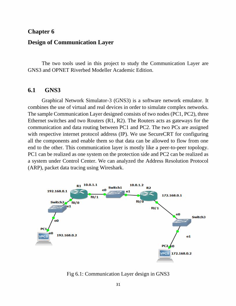
Design of Communication Layer

The two tools used in this project to study the Communication Layer are

GNS3 and OPNET Riverbed Modeller Academic Edition.

6.1 GNS3

Graphical Network Simulator-3 (GNS3) is a software network emulator. It

combines the use of virtual and real devices in order to simulate complex networks.

The sample Communication Layer designed consists of two nodes (PC1, PC2), three

Ethernet switches and two Routers (R1, R2). The Routers acts as gateways for the

communication and data routing between PC1 and PC2. The two PCs are assigned

with respective internet protocol address (IP). We use SecureCRT for configuring

all the components and enable them so that data can be allowed to flow from one

end to the other. This communication layer is mostly like a peer-to-peer topology.

PC1 can be realized as one system on the protection side and PC2 can be realized as

a system under Control Center. We can analyzed the Address Resolution Protocol

(ARP), packet data tracing using Wireshark.

Fig 6.1: Communication Layer design in GNS3

32

6.2 Riverbed Modeller Academic Edition

The Communication Layer for the 6 Bus System under Study is modelled

using OPNET Riverbed Modeller Academic Edition.

Fig 6.2: Communication Layer of Six Bus System

33

6.3 DDOS attack on Communication Layer

i. Network configuration:

The network components are:

- "Attacker" node will conduct the attacks.

- SCADA node "Control Center" will execute remedy actions.

- Server under DDoS attack "Server". This node has its IP address manually assigned

to 192.102.100.1.

- Node_1-6 are the six buses map according to the physical layer.

- All the nodes above are connected to the network through routers and/or switches

and all the nodes in the network can reach each other.

ii. Attack and Remedy settings:

The "Cyber Effects Config" node has the necessary script, attack and remedy

definitions to execute a DDoS attack, and apply a scan/clean remedy action. The

attack and remedy profiles are set as follows. The Attacker has an attack profile

"DDoS Attack" configured to start between 100 and 110 seconds.

DDoS Attack" is defined in the "Cyber Effects Config" node. This attack is

set as follows:

Phase "P1": At the start of the attack, a script is sent to all nodes (e.g. all nodes

supporting Cyber Effects) in an attempt to "infect" the devices, and return a message

back to the "Attacker" indicating if the infection was successful or not.

Phase "P2": 150 seconds after the attack started (~250 seconds simulation time),

another script is sent that instructs the now infected nodes to start sending traffic to

"Server" in an attempt to flood this node. Note that the script in phase "P2" will only

send to those nodes that in the previous phase reported a successful infection. Their

vulnerability settings have an 80% probability of becoming infected if they receive

a malicious infection message from the "Attacker".

34

“Control Center” node has remedy profile "Scan and Clean" configured to start

between 300 and 310 seconds. "Scan and Clean" remedy profile is defined in the

"Cyber Effects Config" node. This remedy has only one phase, which sends a

"Clean" script to all the nodes in the network. The "Clean" script has the effect "Scan

for Infections" configured with a cleaning probability. Those nodes that are

successfully cleaned will stop sending traffic to "Server", reducing the flooding

effect of the attack.

iii. Results:

The Malicious scripts sent by Attacker shows the "Cyber Effects" traffic sent by

"Attacker". The first spike corresponds to phase "P1" of the attack, where the attempt

to infect is made. The second spike corresponds to phase "P2" where the command

to send traffic is distributed to the infected nodes. The level of the second spike is

lower as the second script is only sent to those destinations that get infected by the

first script.

Fig 6.3: Script (traffic) send by the attacker

35

6.4 Global Statistics:

i) All Nodes traffic simulation result

Fig 6.4: Infected devices count and IP Traffic dropped (packets /sec)

6.5 Object Statistics:

i) Server Performance

Fig 6.5: Traffic received by server (packets/sec)

36

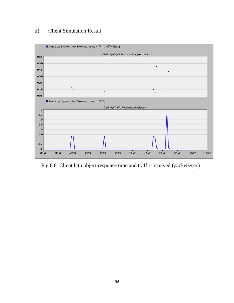
ii) Client Simulation Result

Fig 6.6: Client http object response time and traffic received (packets/sec)

37

Conclusion

Chapter 1, provide introduction on this project and self-healing property of

the smart grids.

In Chapter 2, the System under Study which is a distribution network, the

Physical Layer is modelled using ETAP 16.0.0.

To check if the circuit is converging or not, in Chapter 3, Load Flow studies

and Short Circuit Analysis is performed. Then switching automation is carried out

using in-built Switching Sequence Manager in ETAP 16.0.0 to change the status of

the switches.

In Chapter 4, a System under Study is a Six Bus System. The circuit is

modelled in MATLAB and also Load flow studies is also shown.

In Chapter 5, a controller for the Control Center is built. The algorithm for

State Estimation used here is Weighted Least Square method provided the

measurement data for real and reactive are assumed to be already collected from

PMUs/IEDS. The state vectors to be determined are voltage and bus angles. The

code is written and run in MATLAB and the results is as shown.

In Chapter 6, the Communication Layer can be modelled using two tools

GNS3 and Riverbed Modeller Academic Edition. In GNS3, SecureCRT is used for

configuring all the components and enable them so that data can be allowed to flow

from one end to the other. This Communication Layer is mostly like a peer-to-peer

topology.

A Communication Layer for Six Bus System is modelled using Opnet

Riverbed Modeller Academic Edition. In this model a DDoS attack is introduced by

an external Attacker. The Attacker infect the nodes and flood the Server with the

simulation results showing heavy traffic experience by the Server and the Clients

and the Server performance is bad. The Control Center on the other hand will try to

clean these infected nodes by sending a clean script and heal the system to its normal

state.

38

The CPS has been realized using Intelligent Switching Sequence Management

in the first system under study where during abnormal condition on the power grid,

the system restoration is automated by transferring the load in the off outage area

and transferred to the neighboring feeders through changing the status of normally

–closed (sectionalizing) and normally-open (tie) switches. In the second study case

–Six Bus System a Distributed Denail of Service Attack (DDOS) is performed to

study self-heal property of the system. The simulation results shows that during

attack phase the Nodes are being infected and the Server is being flooded. The Client

Http traffic to access data from the Server is heavy and response time is slow. The

Control Center on the other hand keeps track of the infected Nodes and sends a clean

script to clear the infected Nodes and reduce the traffic on data streaming. Thus, by

intelligent mapping of physical layer to communication layer resiliency of the grid

can be ensured.

39

References

1. Zhuo Su, Luo Xu, Shujun Xin, Weijian Li, Zhan Shi, Qinglai Guo, “Future

outlook of Cyber Physical Power System”, IEEE Conference on Energy

Internet and Energy System Integration (EI2), 2017.

2. Siddharth Sridhar, Adam Hahn, and Manimaran Govindarasu, “Cyber Attack-

resilient Control for Smart Grid”, IEEE 2011.

3. Ching-Tzong Su, and Chu-Sheng Lee, “Network Reconfiguration of

Distribution Systems Using Improved Mixed-Integer Hybrid Differential

Evolution”, IEEE Transaction on power delivery, Vol.18, No.3, July 2003.

4. Sekhavatmanesh, Hossein, Ecole Polytechnique Federale de Lausanne,

“Analytical Approach for Active Distribution Network Restoration Including

Optimal Voltage Regulation” IEEE Journal, Nov 2018.

5. Xinghuo Yu, Yusheng Xue, “Smart Grids: “A Cyber-Physical Systems

Perspective”, May 2016.