CUSTOMS UNION WITH THE EU: GTAP ANALYSIS FOR UKRAINE

by

Oksana R. Harbuzyuk

A thesis submitted in partial fulfillment of the requirements for the degree of

Master of Arts in Economics

National University “Kyiv-Mohyla Academy”

2001

Approved by ___________________________________________________ Chairperson of Supervisory Committee

__________________________________________________

__________________________________________________

__________________________________________________

Program Authorized to Offer Degree _________________________________________________

Date _________________________________________________________

Abstract

CUSTOMS UNION WITH THE EU: GTAP ANALYSIS FOR

UKRAINE

by Oksana R. Harbuzyuk

Chairperson of the Supervisory Committee: Professor Serhiy Korablin

Institute for Economic Forecasting

At National Academy of Science

The thesis analyzes the possible consequences of Ukraine’s integration into the

large European economic structure – European Union. GTAP multi-country

simulation model of Purdue University Center for Global Trade Analysis is

applied. The welfare measure evaluated is change in equivalent variation (EV). As

all incomes in the model accrue to representative household, EV in full assesses

welfare benefit for Ukraine from bilateral tariff elimination on trade with the EU.

As the model includes Ukraine in Former Soviet Union region, EV is estimated

for FSU and then disaggregated on industry level proportionally to trade shares.

The results of simulations suggest that Ukraine’s EV is sensitive to inclusion of

agricultural sector into customs union. Due to highly protected nature of this

sector in the EU, Ukraine is better off if agriculture is excluded from

liberalization. In this scenario Ukraine gains $91.7 millions.

TABLE OF CONTENTS

Table of Contents...............................................................................................i List of Figures....................................................................................................ii List of Tables....................................................................................................iii Acknowledgments............................................................................................iv Abbreviations ....................................................................................................v Chapter 1 Introduction...................................................................................... 1 Chapter 2 Literature review................................................................................4 Chapter 3 Description of Ukraine’s contemporary situation................................9

Copenhagen criteria .....................................................................................9 Progress made by candidate countries ........................................................12 Rapprochment of Ukraine to the EU.........................................................14 Conclusion ................................................................................................18

Chapter 4 Underlying theory and methodology ................................................19 TABLO file in GTAP model.....................................................................20 Expected static gains from tariff reduction: Theory.....................................23 Tariff reduction: How does it work in GTAP?............................................26 Description of simulations performed........................................................32

Chapter 5 Discussion of results ........................................................................35 Analyzing results of simulations .................................................................35 Disaggregating Ukraine’s EV......................................................................40 Comparing base and alternative scenarios...................................................42 Proposals for future research......................................................................43

Chapter 6 Conclusion ......................................................................................45 Works Cited....................................................................................................47 Appendix A: Aggregation of regions ................................................................52 Appendix B: Aggregation of industries.............................................................54 Appendix C: Shocks performed under the first simulation (base scenario) .........57 Appendix D: Shocks performed under the second simulation (base scenario)....61 Appendix E: Trade data used for calculations...................................................64 Appendix F: GDP data used for calculations....................................................67

ii

LIST OF FIGURES

Number Page

Figure 1. The production tree. Presented by Tom Hertel (2001). Adapted from a presentation of Christian Friis Bach. 21

Figure 2. Tree structure of final demand. Presented by Tom Hertel (2001). 22 Figure 3. Trade creation. 24 Figure 4. Trade diversion. 25

iii

LIST OF TABLES

Number Page

Table 1. Equivalent variation, in millions of US$ 35 Table 2. Decomposition of EV, in millions of US$ 36 Table 3. Decomposition of TOT component for FSU, in millions of US$ 37 Table 4. Decomposing allocation effect for FSU, in millions of US$ 38 Table 5. Decomposing trade tariff effects for FSU, in millions of US$ 38 Table 6. Share of Ukraine’s trade in FSU’s trade 39 Table 7. Ukraine’s EV due to TOT, millions of US$ 40 Table 8. EV for Ukraine due to trade tariffs effect, in millions of US$ 41 Table 9. Decomposition for Ukraine of EV due to capital goods as well as

production, input and consumption tax, in millions of US$ 42 Table 10. Summing up EV for Ukraine, in millions of US$ 42

iv

ACKNOWLEDGMENTS

I thank my advisor, Stefan Lutz, for valuable suggestions used in this thesis and

expert guidance; without him this thesis would not exist. Special thanks to

Charles Steele for multiple reading of drafts and corrections made, Roy Gardner

for encouragement and comments. I appreciate support of my colleagues,

especially Oles Chabanovych for help in choosing this topic and ceaseless

espousal, Oleksandr Zholud for essential hints, and Anastasia Shyshkina for

generous inspiration.

v

ABBREVIATIONS

CEECs - Central and Eastern European Countries

CEA – Central European Associates

CGE – computable general equilibrium

EU – European Union

EV – equivalent variation

FSU – Former Soviet Union

INOGATE - Interstate Oil and Gas Transport to Europe

IRTS - increasing returns to scale

GE – general equilibrium

CIF – cost, insurance, freight (INCOTERMS)

GTAP – Global Trade Analysis Project

NIS - New Independent States

NYOE - Number of years open economy

PE – Partial equilibrium

PHARE – Poland and Hungary: aid and economic reconstruction

PTA - Preferential Trading Arrangements

TOT – Terms of trade

TRACECA - Transport Corridor Europe Caucasus Central Asia

WTO - World Trade Organization

1

C h a p t e r 1

INTRODUCTION

Ukraine passed a tremendous period of its history in the 20th century. And

after collapse of Soviet Empire it recovered more slowly than did the Baltic

States and still more slowly than what used to be called Central and Eastern

European Countries (CEECs). Only in 2000 did GDP begin to rise after a

decade of decline1. Strong state regulation of foreign trade was obvious in

1994. In 1999, there still were no signs on the date Ukraine would join World

Trade Organization (WTO) (see, e.g., Michalopoulos (1999)); and the

country was treated as a non-market economy by this organization2.

Some changes came in 2000. The European Union recognized Ukraine as a

market economy in dumping treatment in October; and the WTO announced

Ukraine could be accepted in 2001 if its Parliament approves changes to

nearly 60 laws and provisions by that time (Postup, 2000d).

The way Ukraine’s western neighbors followed has been to apply for

acceptance into a large European integration structure – the European Union

(EU). The EU puts the following requirements for potential candidates

(Copenhagen European Council, 1993):

1 The growth is reported at 6% for this year (Postup,2001). See also Business Central Europe (2001).

2 This means in considering dumping cases by its partners, costs of Ukrainian producers were not calculated from their actual costs but taken from comparable producer in other, market -economy country. The argument behind this is that non-market economy implicitly subsidises its producers, e.g. through supplying them with cheap energy. Such procedure of treating led to more judgements to detriment of Ukrainian producers.

2

• Democratic regime, protection of minorities’ rights, respect for human

rights

• Market economy, competitive industries capable to compete with

European ones

• Readiness to accept aquis communautaire (about 80 000 pages of law, which

regulates EC’s life (Price and Landau, 2000))

Despite the fact that Ukraine has poor economic and, especially recently,

political performance3, it is encouraged to integrate into international trade

structures. So, in 1994 Partnership and Co-operation agreement with the EU

was signed, which envisioned creation of customs union (CU) in 1998. As

economic conditions were not appropriate then, CU was postponed. If

Ukraine finds a way around its political crisis successfully and retains the

trend in economic growth, CU will be of relevance again. That is my

motivation for assessing its impact on welfare of Ukraine.

Economic theory suggests that there will be trade diversion after Ukraine’s

trade partners enter the EU, which means Ukraine’s firms will lose ties with

some of their counterparts in those countries. Further, Chang and Winters

(1999) demonstrate that if a country enters Preferential Trading

Arrangements (PTA) “other contracting parties [who fail to enter it] may ….

be affected adversely, because they are compelled to reduce their prices to

meet competition from the suppliers within the PTA” (pp.33). Two of

Ukraine’s top-5 trade partners are preparing to enter the EU – Poland and

Turkey4. Besides, the EU is the largest of Ukraine’s trade partners outside the

3 The EU provides a figure for Ukrainian GNP per capita for year 1999 $700. Political situation was

particularly worsened by restrictions to freedom of speech in connection with case of Gongadze.

4 The top-5 Ukraine’s trade partners are ranging as follows (1998): Export – Russia, China (steel), Turkey, Germany, Belarus Import – Russia, Germany, US, Poland, Italy

3

Newly Independent States (NIS); and the trade volume with it is growing

from year to year at the expense of the NIS.

In this thesis I want to show that Ukraine’s acceptance into the EU not only

will help to avoid trade diversion with some partners, but also will foster trade

creation and increase in welfare (evaluated with equivalent variation (EV)).

For this purpose, the GTAP multi-country simulation model of Purdue

University Center for Global Trade Analysis is used. This is a perfect

competition, constant returns to scale (CRTS) model with Armington style

specification of imports and nested structure of demand and supply.

The Computable General Equilibrium (CGE) model GTAP is applied to

calculate results of bilateral tariff reduction. Ukraine is still not disaggregated

in version 4 of this model; that is why computation is actually done for the

Former Soviet Union (FSU). Then EV is disaggregated proportionally to each

Ukrainian industry’s share in total trade of FSU industries.

The thesis outline is as follows. The next chapter elucidates the state of

literature on economic integration, trade, growth, and Ukraine. This includes

overview of writings on theory as well as empirical methods and previous

studies. Chapter three should familiarize the reader with progress in the EU-

Ukraine relations. It also includes the background of the EU-Candidate

countries negotiations and description of accession criteria. Subsequently,

Chapter four is designed to present analytical model of Purdue University

Center for Global Trade Analysis. Also, it shows theoretical underpinning of

consequences of formation of customs union and step-by-step derives change

in EV from bilateral tariff elimination. Chapter five gives an assessment of

results obtained, sensitivity analysis, and suggestions for future work. Finally,

the last chapter draws a conclusion to the work.

4

C h a p t e r 2

LITERATURE REVIEW

This chapter presents a review of the recent literature on economic

integration, followed by a survey of studies on growth and trade. It concludes

by assessing the relevant literature on Ukraine.

There are two approaches to estimation of gains from liberalization. The first

is to assess static gains (Kose and Riezman, 2000; Chang and Winters, 1999).

The second is to approximate dynamic benefits. The first approach is more

elaborated and, actually, less sophisticated.

Kose and Riezman (2000) use a computable general equilibrium (CGE)

model to analyze two large and one small country case. They are interested in

finding better policy choices for the small country. The options that each of

the countries faces are Free Trade Agreement (FTA), Customs Union (CU),

and free trade (FT). The findings suggest that the best outcome for the small

country is FT. Under FTA setting the country prefers to be an “innocent

bystander”. This means that the country favors being left out of the FTA to

forming coalition with one of the large countries. Finally, costs of being

“bystander” become harder if FTA between two large countries is substituted

for CU. Now, the small country would prefer CU with one of two large

countries to staying alone.

This work is valuable to my thesis because it suggests handy methodology –

CGE – and sets theoretical grounds for expected implications for welfare of

CU for small country. Albeit, it uses compensating variation (CV) for welfare

measurement, while I employ equivalent variation (EV). The difference is that

I intend to assess how much country gains in current prices, while CV shows

welfare benefit in new equilibrium prices.

5

Another study on CU is Chang and Winters (1999) that deals with the

problem of trade distortions in MERCOSUR, a customs union of Argentina,

Brazil, Paraguay, and Uruguay. The authors develop a two-firm Bertrand

pricing game – with an insider and an outsider. The first benefits from

his/her country inclusion into a customs union because of possibility of

increasing prices (no tariffs and higher demand), while the latter loses from

exclusion and lower demand. The empirical study, based on the model,

revealed losses of Brazil’s main importers (countries that export to Brazil) in

1996 - USA ($624.1 million), Japan ($58.8 million), Germany ($236 million),

Chile ($17.3 million).

This study is useful for my research in that it states the fact that left out of CU

country not only has opportunity costs – foregone increase in welfare – but

also real damage from losing export markets.

Harrison et al (1996) employ a CGE model of their own to assess implications

for Turkey of customs union with the EU. Their model contains three

regions – Turkey, the EU, and rest of the world. The model has nested

structure, CRTS, and CES function for description of private consumption.

The novelty of the model consists in disaggregating capital (5 types) and labor

(8 types). The authors find that Turkey should gain about 1 to 1.5 % of GDP,

mainly due to improved access to third countries markets. At the same time, it

is supposed to lose about 1.4 % in decreased tariff revenues. The replacement

tax the authors propose is value-added tax (VAT), applied uniformly to all

agents. The study is useful for my work, because the authors provide a

comparable research to what I intend to do, although for different country.

Hertel et al (1997) present a CGE model that is publicly available. In contrast

to Kose and Riezman (2000), their GTAP model is based on real data for the

world. Version 4 of it incorporates 45 regions and 50 industries with input

output (IO) tables and trade flows reported by countries. The model has

nested structures of demand and supply, includes government sector and

6

employs constant difference of elasticities (CDE) function for treating private

expenditures. My research bases mostly on this theory, which is why it is

important to include it here.

The second approach, dynamic in nature, is represented by econometric

techniques and CGE model. This approach is mostly concerned with

assessing changes in growth rate of liberalizing regions.

Wacziarg (1998) is an example of recent investigation on whether trade

liberalization influences growth. The author develops a new index of trade

policy openness and uses it in simultaneous equation system for a panel of 57

countries to confirm strong positive relationship between trade liberalization

and economic growth. The article is criticized by Rodrigues and Rodrik

(1999) because of averages constructed over just 5 years (the authors would

prefer 10 year horizon). They also argue it would be more interesting to see

results, based on indicators of trade policy like tariffs or non-tariff barriers

(NTB).

These articles as well as the next three papers are interesting for me, because

they show recent advances in literature to the question of trade liberalization

effects and call for further elaboration of my thesis.

An author, who undertakes effort to identify all significant sources of growth,

is Sala-I-Martin (1997). He proposes for discussion his results gotten from

running more than 30,000 regressions. The test is designed to answer the

question: which of 60 examined variables are strongly related to growth. As

contrary to the claim “Nothing is Robust”, Sala-I-Martin finds 21 variables to

be strongly related to growth, when extreme bound analysis is avoided. The

variable “Number of years open economy” (NYOE) is among the variables

with the best explanatory power, while other trade-openness variables seem

to be insignificant.

7

The above investigation is elaborated in Doppelhofer, Miller, and Sala-I-

Martin (2000). Because of stricter requirements to data they test only 32

variables on their correlation with growth. A novel technique, namely

Bayesian Averaging of Classical Estimates, is employed to assess the

robustness of the variables, 11 of which prove to be robustly related to

growth. Regional, religious, and human capital variables as well as log of GDP

per capita are among survivors. Along with NYOE, “Fraction of Primary

Exports in Total Export” appears to be significant, though with negative sign.

However, the authors admit that their model allows only for a linear

relationship. Notably, the data do not include any of the former Central

Planning Economies (CPEs).

Baldwin and Forslid (1998) explain that insignificance of trade liberalization

and growth link in results of other authors is due to non-linearity of this

relationship. The authors bring forward an argument of Rivera -Batiz and

Romer (1991), which suggest that gradual liberalization from autarky to free

trade first decreases and then raises growth. Baldwin and Forslid develop a

simple innovation based growth model and estimate impact on growth of

different (ad valorem and specific) tariff and non-tariff barriers. Their model is

consistent with U-shape relationship between ad valorem tariffs and growth;

they find it to be bell-shaped for specific tariffs and insignificant for technical

barriers in case of small import of inputs to R&D sector.

Hertel et al (1997) use perfect competition and constant returns to scale

(CRTS) in all industries, although the model allows for alteration in those two

assumptions. Rutherford and Tarr (1998) propose a model with large group

monopolistic competition and increasing re turns to scale (IRTS) in industries

producing intermediate commodities. They construct 2 goods sector

economy where goods interact through Dixit-Stiglitz function. The advantage

of this paper is that it allows to ex ante estimate dynamic gains from

liberalization. The authors apply their model to five small countries and

8

emphasize the finding that the resulting from liberalization growth crucially

depends on free movement of capital.

Literature on Ukraine, its growth and possible integration in the EU is not

very abundant. This is, e.g., represented by Kaufmann (1997) and Hoffmann

and Moellers, ed. (2001). Kaufmann discusses obstacles to growth in Ukraine,

while the book of Hoffmann and Moellers concerns the place of Ukraine in

contemporary Europe, discusses the role of Partnership and Co-operation

Agreement (1994) for Ukraine, and also projects influence of eastern

enlargement of the EU on Ukraine.

9

C h a p t e r 3

DESCRIPTION OF UKRAINE’S CONTEMPORARY SITUATION

In this chapter I first describe the documents, which address the question of

European Eastern enlargement. In this part, the three requirements to EU

candidates are summarized and clarified. The discussion is based on three

original sources: The Presidency Conclusions of Copenhagen and Helsinki

European Councils and the Composite Paper of the European Commission.

Second, a general picture is given on how Ukraine’s Western neighbors meet

the Copenhagen criteria, their policies pursued and documents applied. Again,

the use is made of the Composite Paper of European Commission. Third, the

state of play in Ukraine is elucidated and relevant summaries of three basic

documents in this field are being made, i.e. Partnership and Co-operation

Agreement, European Council Common Strategy on Ukraine, and Program

of Integration into the EU.

Copenhagen criteria

In response to a large number of countries applying for accession to the

European Union, the European Council adopted the Copenhagen criteria in

June 1993. These are explicit requirements that the candidate countries should

meet in order to become full members of the EU. The criteria can be split in

three areas: political, economic and acquis-related5. They are described as

follows:

“Membership requires that the candidate country has achieved stability of institutions guaranteeing democracy, the rule of law, human rights and respect

5 Acquis is about 80,000 pages of directives and regulations adopted in the European Union since Treaty

of Rome (1957) (Price and Landau, 2000).

10

for and protection of minorities [political criteria], the existence of a functioning market economy as well as the capacity to cope with competitive pressure and market forces within the Union [economic criteria]. Membership presupposes the candidate's ability to take on the obligations of membership including adherence to the aims of political, economic and monetary union [acquis-related criteria]”(7.A).

The political criteria are consistent with Article 6 of the Amsterdam Treaty:

“The Union is founded on the principles of liberty, democracy, respect for

human rights and fundamental freedoms and the rule of law”. Furthermore,

the Helsinki European Council stresses that meeting these cri teria “is a

prerequisite for the opening of accession negotiation” (I.4).

The Commission has construed the economic criteria in Agenda 2000 as “the

existence of a functioning market economy” and “the capacity to cope with

competitive pressure” (Article T). The existence of a functioning market

economy in Composite Paper (June 1999)6 is judged by the following:

• Equilibrium between demand and supply is influenced only by market

forces

• Trade and prices are liberalized

• Barriers to market entry and exit are not significant (transparent

legislation on business establishment and bankruptcy)

• Effective enforcement of legislation on property rights

• Macroeconomic stability (low inflation, public debt, and budget deficit)

• Developed financial sector

The capacity to withstand the competitive pressure within the Union in the

same paper is subdivided as follows:

• Economic agents are able to make macroeconomic decisions in stable and

predictable environment

6 Reports on progress towards accession by each of the candidate countries.

11

• Developed infrastructure (transport, energy sector, telecommunication) in

place

• Properly trained and educated labor force

• Ample spending on research and development by country

• Weighted government role in trade and competition policy, state aid,

support for SMEs

• Significant trade volume of appropriate nature with the Union

• Large proportion of small firms, which are flexible enough to withstand

competition

The Helsinki European Council (1999) states that ”[p]rogress in negotiations

must go hand in hand with progress in incorporating the acquis into legislation

and actually implementing and enforcing it.” Acquis is divided in 31 chapters

for candidate countries:

November 19987(7 chapters): science & research, education & training, small

& medium-sized enterprises, culture & audio-visual policy,

telecommunications, industrial policy, common foreign & security policy;

First semester of 1999 (8 chapters): company law, statistics, consumer &

health protection, fisheries, competition policy, free movement of goods,

customs union and external relations;

By the end of 19998 (8 chapters): social policy, EMU, free movement of

capital, energy, transport, taxation, freedom to provide services and

environment;

By the end of June 2000 (7 chapters): agriculture, regional policy, free

movement of persons, justice & home affairs, financial control, financial &

budgetary provisions and institutions.

7 The date, when respective chapters were opened

8 The date, when appropriate chapters were intended to be opened

12

Progress made by candidate countries

13 countries applied for EU membership and became candidates in the

1990s: Poland, Hungary, the Czech Republic, Estonia, Slovenia, Cyprus,

Slovakia, Latvia, Lithuania, Malta, Bulgaria, Romania, and Turkey (European

Commission, 1998). If Ukraine applies it will have to pass the same procedure

as described below.

The relations of the EU with each of the candidate countries are based on the

Accession Partnerships and Europe Agreements. The Accession Partnerships

set out the short and medium term priorities for preparation to EU accession.

They also allocate financial assistance from the EU (3 billion euro a year from

2000). The Europe Agreements establish and guide functioning of

Association Councils, Committees and sub-committees, which oversee the

pre-accession process in the candidate countries. Each of the candidate

countries has also approved its national program for the adoption of the

acquis.

All candidate countries from Central and Eastern Europe participate in the

programs of the Union on education, training, youth, culture, environment,

energy, research, and SMEs.

The financial support of the EU is split in three programs from the year 2000:

PHARE, ISPA, and SAPARD. PHARE9 (1.5 billion euro yearly) is aimed at

financing institution building and investments in acquis in the candidate

countries. An example of the latter is financing computerization of the eastern

border of Poland or equipment of testing laboratories in the Czech

Republic10. Two other programs are structural funds, of which ISPA (1billion

9 Poland and Hungary: aid and economic reconstruction.

10 Composite Paper.

13

euro) allocates funds to transport and environmental protection and

SAPARD11 (500 million euro) – to agriculture and rural development.

The European Commission prepared questionnaires in April 199612, which

became the basis for opening negotiations with the first-wave five countries

(Poland, Hungary, the Czech Republic, Estonia, Slovenia). Slovakia failed to

meet political criteria. Cyprus was added to the negotiation list shortly

thereafter. Official date of opening negotiations is March 1998. The

negotiations pass in the form of bilateral accession conferences, during which

progress on conforming to open chapters (see the previous page) is discussed.

Simultaneously in April 1998, the Commission started the process of

screening for candidate countries, i.e. explaining legislation of the EU. In

1999, some officials of the Commission forecasted Accession Treaties to be

signed for the most advanced candidates in the year 2000 (Franco, 2000,

p.75), but as for now the date is postponed till 2002. On the one side, the

Commission doesn’t want to bring the loss of momentum. On the other, it

wants the newcomers to become full Members, so it faces a trade-off.

What are the main obstacles in accession for the candidates? First, this is a

poor political environment in the candidate countries. Slovakia was close to

meeting the Copenhagen criteria in 1996 if not for “Prime Minister Meciar’s

antics and undemocratic methods“ (Price and Landau, 2000, p.17). In

November 2000, EU Enlargement Commission Guenter Verheugen

declared that two of the second-wave candidates caught up with the first

wave candidates. So, the division in waves is no longer meaningful. Though

the two successful countries were not announced, EU representatives

singled out Slovakia and Malta in the past (Eubusiness, 2000a). Other

political criteria to be overcome are the mistreatment of minorities in Latvia

11 The program is foreseen for years 2000-2006, in November 2000 EUR 520 are available (Composite

Paper, 1999).

12 The questionnaires comprised 150 pages of questions, which the applying countries had to answer in three months. Some answers amounted to 1,500 pages.

14

as well as unsatisfactory childcare and Roma treatment in Romania

(Composite Paper, 1999).

Second, most of the candidates face financial difficulties. For instance,

different experts mention sum of 30 to 40 billion of ECU for application of

environmental regulations of acquis in Poland and ECU 120 billion for the

first-wave candidate countries, except Cyprus, together (Cosgrove-Sacks,

2000, p. 61).

Further, the question of nuclear power safety is of great concern for the EU.

For the moment, three of the candidate countries have non-upgradeable

reactors, namely Lithuania, Slovakia and Bulgaria. Slovakia already

committed itself to close its units in 2006 and 2008; Lithuania will close one

unit in 2005 and decide on the second in 2004. Only Bulgaria is still not

prepared to decide anything on this matter (Composite Paper, 1999).

Finally, economic development statistics in candidates show greater variability

in 1998-1999 because of Asian and Russian crisis. The countries that still

have substantial ties with Russia were affected considerably by Russian

financial crisis. As reforms in Romania were sluggish, its economic growth

dropped to –7.3% in 1998 and –5% in 1999. Poland and Hungary endured

the crisis most easily - 5.1% and 4.8% growth in 1998 respectively and

about 4% in 1999 (Composite Paper, 1999). This is a crucial question as the

candidate countries had GDP per capita 18% (Latvia) to 62% (Cyprus) of

the EU average in 1996 (The Economist, 1997) and can only catch up through

growing more quickly.

Rapprochment of Ukraine to the EU

“Any European state may apply to become a Member of the Union. It shall address its application to the Council, which shall act

15

unanimously after consulting the Commission and after receiving the assent of the European Parliament, which shall act by an absolute majority of its component members.”

Article O of the Treaty of Rome (now article 49 of the Amsterdam Treaty)

The basis for EU-Ukraine relations was laid down in the Partnership and Co-

operation Agreement (PCA) on 14 June 1994. Ukraine was the first of the

Newly Independent States (NIS) to sign this kind of document with the EU

to replace former Agreement on Trade and Commercial and Economic Co-

operation with the USSR. The aim of the Parties to the document is to

establish a free trade area between them starting from year 1998 if appropriate

(Article 4 of PCA). According to the Agreement, the Parties grant to each

other most-favored-nation (MFN) treatment and the products of the other

party should not be subject to discriminatory direct or indirect taxation, i.e.

higher taxed than domestic products (A10 and 15 respectively). However,

textile and steel products are exempted from the latter clause. Further, the

Agreement encourages “the approximation of Ukraine’s existing and future

legislation to that of the Community” (A51). The areas, the co-operation will

concentrate, are close to the 31 chapters for negotiation with the candidate

countries (see end of part I of this chapter):

“industrial cooperation, investment promotion and protection, public procurement, standards and conformity assessments, mining and raw materials, science and technology, education and training, agriculture and agro-industrial sector, energy, civil nuclear sector, environment, transport, space, telecommunications, financial services, money laundering, monetary policy, regional development, social co-operation, tourism, small and medium-seized enterprises, information and communication, consumer protection, customs, statistical co-operation, economics and drugs”13 (Article 52 of PCA).

13 Article 52.

16

The newly created Co-operation Council is entrusted with the supervision

duty on the Agreement (A85). Other established institutions are the Co-

operation Committee and the Parliamentary Co-operation Committee. The

Agreement is concluded for ten years to be renewable on a year-by-year basis

(A101). Except for Articles 30 (on companies) and 59 (on education) this

document seems to be very equitable14.

The next step in the EU-Ukraine relations was the adopted by European

Council Common Strategy on Ukraine (December 1999). In this document,

“[t]he EU acknowledges Ukraine’s European aspirations and welcomes

Ukraine’s pro-European choice” (A6). Likewise, “[t]he European Council

recognizes that a successful, stable and secure Ukraine is in the best of

interests of the EU” (A7). Further, the European Council reminds Ukraine of

all the Conventions it has signed and all the commitments it has made,

especially those with the Council of Europe in 199515 (A12). Finally, the EU

promises to foster development of infrastructure networks in Ukraine

through its TACIS programs (INOGATE and TRACECA16) and to assist in

the transmission of Euronews on Ukrainian television by June 2000 (A37, 50

and 65).

Ukraine started to actively strive for the EU membership at about that time

(1999), providing its foreign policy accordingly (James, 1999a, 1999b;

Partridge, 1999). In September 2000 Program on Ukraine’s Integration into

the European Union was signed. The program prescribes Ukraine’s strategy

in the following important areas: democracy and rule of law, court system,

human rights and protection of minorities’ rights, economic development of

14 So, Ukraine should provide to EU enterprises environment comparable to its own businesses (not

worse), while the EU agrees to provide best environment given to other non-EU countries (maybe, worth than its own EU businesses). Also, cooperation on studying Ukrainian culture and language as well as training interpreters in the EU is not foreseen.

15 Ukraine attained membership in the Council of Europe on 9 November 1995

16 Interstate Oil and Gas Transport to Europe

and Transport Corridor Europe Caucasus Central Asia

17

the country, internal market without borders, economic and fiscal questions,

sector policy, social harmonization, regional policy and co-operation, living

standards and environmental protection, innovations, information policy,

education and youth, justice and domestic affairs, foreign-economic activity,

foreign and security policy, administration opportunities, and financial

questions. In the document Ukraine affirms its commitments to the Council

of Europe; inter alia, it reminds of canceling death penalty (A4.1.2). Further, it

emphasizes its economic stabilization – industrial growth of 4.3%, inflation

rate 19.2%, budget deficit 1.5%, and positive trade balance in 1999 - and

highlights its objective to gradually increase investments to 27% of GDP in

2010(A5.1). It also announces its intention to encourage trade “far abroad”,

up to 60% of total trade in foodstuffs in 2005 (A8.2.5).

Ukraine’s relations with the World Trade Organization (WTO) and Central

European Free Trade Association (CEFTA) deserve a separate paragraph

because Ukraine holds them as crucial in its pre-accession strategy (A16.1.1,

16.1.2). Currently, Ukraine holds the status of an observer with the prospect

of becoming full member in 2001 in case it brings all the necessary

harmonization to its legislation17. For the moment, Ukraine stands in bilateral

negotiations on market access with almost 30 countries. The negotiation

partners include EU, US, Japan, Canada, Australia, CEFTA Members, etc.

CEFTA was established in March 1993 by Visegrad Three (Hungary,

Czechoslovakia, and Poland) (Program on Ukraine’s Integration, 2000). The

Visegrad Three became the Visegrad Four after Czechoslovakia’s breakup;

and three more countries joined CEFTA from 1996 to 1998 (Slovenia,

Romania, and Bulgaria). The criteria for joining the group are as follows:

• Associated membership in the EU

• Membership in the WTO

17 The Deputy Economy Minister’s words as in Postup’s Infobank, 11 October 2000

18

• Agreements on free trade being signed with every Member Country

CEFTA members trade 90% of their mutual trade volumes duty-free

(Program on Ukraine’s Integration, 2000) and are looking forward to new

members accession. Ukraine, eager to escape a fall in its trade with those

countries after their accession to the EU, strives for CEFTA accession as

soon as possible. It has already signed program documents on trade

liberalization with five of the countries, memorandums being also handed

over to Slovenia and Romania.

Conclusion

Ukraine has made some progress in the process of rapprochment to the EU.

The European Council gave Ukraine the status of a country with market

economy in October 2000 (Postup, 2000a). In November 2000, Ukrainian

lawmakers approved a program to harmonize Ukrainian legislation with

Europe’s. A Commission for European Integration will be established to

verify the conformity of Ukrainian laws with European laws (Postup, 2000c).

The advances were positively evaluated by Mr. Romano Prodi (2000),

President of the European Commission, during his visit to Ukraine:

“Ukraine has stated clearly that its goal is closer integration with the European Union. The EU, in the Common Strategy, has acknowledged Ukraine’s European aspirations and welcomed Ukraine’s pro-European choice.”

The legislative improvements are being supported by progress in

development of industrial co-operation between Ukraine and the EU, which

evidences increased competitive strength of Ukrainian goods (Postup, 2000b,

2000d).

19

C h a p t e r 4

UNDERLYING THEORY AND METHODOLOGY

In my work, I am going to answer the following question: how will Ukraine

benefit from joining the EU. As Rutherford and Tarr (1998) suggest, static

gains often underestimate real benefit from liberalization and, thus, dynamic

estimates would be more precise. Further, Hertel (2001) argues that general

equilibrium (GE) analysis allows for controlling effects of liberalization in

one market on the rest of the markets and, in this way, GE analysis has its

advantages over partial equilibrium (PE). Applied general equilibrium (AGE)

models also take account of resource constraints for economy.

The best model to suit for calculations would be dynamic version of Global

Trade Analysis Project (Dyn-GTAP). That model of Purdue University

Center for Global Trade Analysis takes time as continuous variable in capital

accumulation equation, permits capital mobility among regions to adjust for

difference in risk-free interest rates, hence approximating long-run

equilibrium. The user can perform a series of simulations with controlled path

of tariff reductions for a desirable number of years. Unfortunately, the model

is not available publicly for the moment.

Consequently, I will have to restrain myself to estimation of static result from

tariff reduction, i.e. short-run equilibrium result. Ordinary GTAP model can

serve this purpose, version 4. The main difference from Dyn-GTAP is

absence of time variable. This version includes 45 regions and 50 sectors,

which result in more than 20 000 variables in more than 15 000 equations.

The data in the model is updated for year 1995.

20

TABLO file in GTAP model

All the theory GTAP builds on is contained in the TABLO file. The

underlying theory in the model is as follows. First, perfect competition is

assumed in all sectors. Some authors (Rutherford and Tarr, 1998) prefer large

group monopolistic competition (MC) in the intermediate sector. Basic

argument for this could be high fixed costs for starting business in this sector.

High fixed costs call for mark-up in the industry, which is not possible in

competitive industry but is consistent with monopolistic competition. Second,

Hertel and Tsigas (1997) employ constant returns to scale (CRTS) for all

sectors, while increasing returns to scale (IRTS) are imposed upon

intermediate sector by Rutherford and Tarr (1998) for the same line of

reasoning as MC. Large fixed costs result in ever decreasing average costs and

economy of scale. Both suggestions of Rutherford and Tarr seem to be

reasonable, but those required changes to GTAP demand more

time/expertise than is available for this work.

Further, Hertel and Tsigas (1997) employ Armington style product

differentiation. This means, consumers differentiate among products of

different origins and the country imports according to formula (Geraci and

Prewo, 1982):

)1/(/)1(

−

≠

−

=′ ∑

rr

rr

riirirr xam

σσσσ for r, i=1, 2, …, n

where

m’r = quantity index of total imports into r (prime indicates CES

functional form);

xir = quantity of imports into country r from country i;

air = weight multipliers;

σr = elasticity of substitution between any two imported products of

different origins (σ > 0);

21

n = total number of countries.

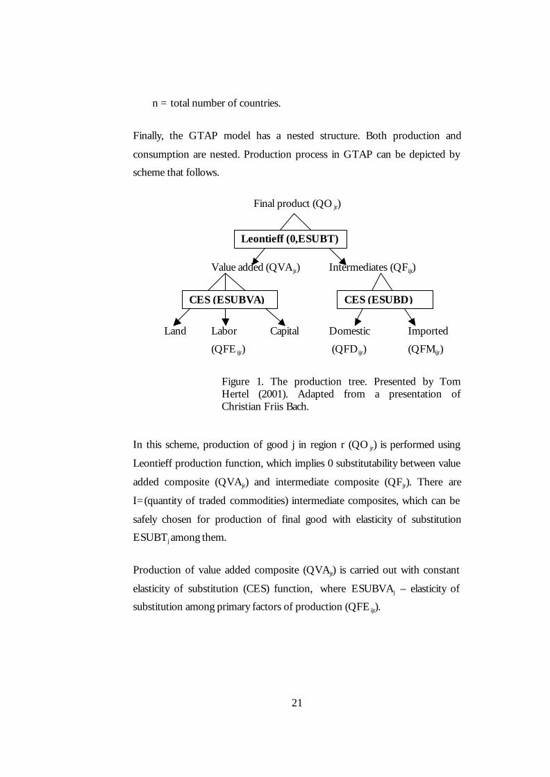
Finally, the GTAP model has a nested structure. Both production and

consumption are nested. Production process in GTAP can be depicted by

scheme that follows.

Final product (QO jr)

Value added (QVA jr) Intermediates (QFijr)

Land Labor Capital Domestic Imported

(QFE ijr) (QFDijr) (QFMijr)

Figure 1. The production tree. Presented by Tom Hertel (2001). Adapted from a presentation of Christian Friis Bach.

In this scheme, production of good j in region r (QO jr) is performed using

Leontieff production function, which implies 0 substitutability between value

added composite (QVAjr) and intermediate composite (QFjr). There are

I=(quantity of traded commodities) intermediate composites, which can be

safely chosen for production of final good with elasticity of substitution

ESUBTj among them.

Production of value added composite (QVAjr) is carried out with constant

elasticity of substitution (CES) function, where ESUBVAj – elasticity of

substitution among primary factors of production (QFE ijr).

Leontieff (0,ESUBT)

CES (ESUBVA) CES (ESUBD)

22

Finally, the intermediate composite is produced from domestic good (QFDijr)

and import composite (QFMijr or m’) with CES production function

(elasticity of substitution ESUBDi).

The production process is performed under assumption of separability, which

means that optimal mix of land, labor, and capital (QFE ijr) doesn’t depend on

prices of intermediates. Thus, solution procedure has two steps: firstly, we

choose optima l mix of primary factors of production and optimal mix of

domestic and foreign goods and, secondly, we choose optimal intermediate

composite for production of final good.

Nested structure of demand takes the following form:

Per Capita Utility (U)

Private expenditure Savings Government expenditure UP QSAVE/POP UG

qp(“1”)…qp(“i”)…qp(“n”) qg(“1”)…qg(“i”)…qg(“n”) Individual commodities

Figure 2. Tree structure of final demand. Presented by Tom Hertel (2001).

Consumer derives utility from private expenditure (UP), savings

(QSAVE/POP), and government expenditure (UG) according to Cobb-

Douglas utility function. Inclusion of savings in static model bases on the

work of Howe (1975) as in Hertel and Tsigas (1997, p.46), who has shown

that intertemporal expenditure system can be derived from static

maximization problem with savings. Government Cobb-Douglas expenditure

(UG) are executed with constant share of outlays for each good (σ=1, i.e. in

Cobb-Douglas, σσ=1

Cobb-Douglas

CDE

23

( ) ( )1221 PPQQ=σ 1% increase in ratio of prices is compensated by 1%

decrease in ratio of quantities). Inclusion of UG into households’ utility is

motivated by the work of Keller (1980) as in Hertel and Tsigas (1997, p.47).

Finally, private expenditure function has constant difference of elasticities

(CDE) form, originally suggested by Hanoch (1975).

Why CDE? Cobb-Douglas and CES are inconsistent with real data because

they are homothetic, i.e. expenditure shares spent for particular goods are

independent on level of income. Thus, there would be no possibility for

luxury goods, which is unrealistic. The function that allows for change not

only in expenditure shares but in marginal expenditure shares (observed in

real life) is CDE (Huff et al, 1997). CDE lies halfway from CES to fully

flexible form function (i.e. one defined in point by fixing second derivative in

that point).

Expected static gains from tariff reduction: Theory

Why should tariff reduction bring welfare gain to a country? International

trade studies answer this question in two categories: trade diversion and trade

creation. Trade creation unambiguously produces welfare gain, while trade

diversion is vague in sign of welfare change. Let’s look at them closer.

Trade creation arises under customs union (CU) formation if a country

engages in trade in a good it didn’t trade in before.

24

Figure 3. Trade creation.

On the graph above, the country has prohibitive tariff t on the good, which

causes Rest of the World (Pw’) and EU (Pe’) supply prices to be higher than

domestic equilibrium price (P*). That’s why the country doesn’t trade that

good. After it forms customs union with the EU, it eliminates tariff t on EU’s

goods and the price lowers below domestic price (P*) to Pe. Consumer

surplus in the country increases from vinous triangle to a bigger upper triangle

bordered with a bold line. The difference between those two triangles (change

in consumer surplus) is equal to equivalent variation under quasilinear utility

function. Initial producer surplus of the country, marked red, decreases to the

lower bordered with bold line triangle. Net gain for the country is the hatched

triangle. Note that it is not the most efficient outcome as the country uses less

efficient supplier (with higher costs) but it is better in terms of efficiency than

initial equilibrium. Thus, we would expect allocation of resources in the

country to improve. Together with better terms of trade (TOT) it would

source increase in welfare.

Trade diversion is switching from cost-effective partner to ineffective one, i.e.

the country trades in the same good but with a different partner.

25

Figure 4. Trade diversion.

On the graph above, the country maintained tariff rate t, which was

prohibitive for the EU but not for Rest of the World. Thus, the country

imported some of the good from the Rest of the World (ROW) at price Pw’

and gathered import duty equivalent to the area of yellow rectangular. There

was no trade with the EU. Consumer surplus (CS) was equal to the area of

vinous triangle and producer surplus (PS) corresponded to the red triangle.

Now, that the country forms a customs union with the EU, it eliminates

import tariff t for the EU. The equilibrium price falls to Pe. At once, there is

no import of the commodity from ROW but only from the EU. Consumer

and producer surpluses change to the areas bounded with bold line; tax

revenues for the country disappear. On the net, the country gains two

hatched triangles and looses hatched part of the yellow rectangular. As the

things are, gains prevail, but if Pe rises or Pw decreases the hatched rectangular

becomes larger and two triangles can decrease so that loses come to

overweigh gains. Hence, change in consumer surplus (under quasilinear utility

– EV) is positive and overall effect is ambiguous. Note partial equilibrium

26

(PE) nature of analysis in this section. See Suranovic (1999) for detailed (PE)

treatment of the topic.

In GTAP, all the income, including taxes, accrues to consumers. That’s why

EV encompasses change in both CS and PS as well as government revenue

and equals total effect of trade creation or trade diversion. Its sign is

ambiguous. The formula for EV in the model is (Hertel and Tsigas, 1997,

p.61):

EV(r) = u(r) * INC(r) / 100,

where u(r) = percent change in per capita utility (see Figure 2);

INC(r) = income of region r before simulation.

As population shocks are possible in GTAP, the final equation takes more

sophisticated form. I won’t present it here because in my simulations

population is held constant.

Tariff reduction: How does it work in GTAP?

When Ukraine enters into a customs union with the EU, both eliminate

bilateral tariffs on all goods (eventually). Let’s consider in details how

elimination of tariff on import of good i from the EU to Ukraine influences

general equilibrium (Hertel and Tsigas, 1997, p.45-46). A remark should be

made that uppercase letters define absolute changes (X), while lowercase

letters label mostly relative changes (x=ÄX/X) in GTAP. Concerning import

tariffs, uppercase letters mark power of the tax (T) – ratio of domestic

(market) price to world price. T>1 in case of import tax and T<1 in case of

import subsidy. Again, lowercase letters mark change in the power of the tax.

I will adhere to GTAP designation.

27

Elimination of bilateral import tariff on good i will decrease the tariff to 0

(decrease the power of import tax to 1). It will lower price of good i in

Ukraine according to equation:

pms(i,EU,Ukr) = tm(i,Ukr) + tms(i,EU,Ukr) + pcif(i,EU,Ukr), (1)

where pms(i,EU,Ukr) = change in domestic (market) price in Ukraine of

commodity i imported from the EU

tm(i,Ukr) = change in power of the source-generic import tax on

imports of commodity i in Ukraine

tms(i,EU,Ukr) = change in power of the tax on imports of

commodity i from the EU to Ukraine

pcif(i,EU,Ukr) = change in world price of commodity i imported

from the EU to Ukraine

In the equation, tm(i,Ukr)=0 (this tax doesn’t change), tms(i,EU,Ukr)<0 (this

tax is eliminated), and pcif(i,EU,Ukr)=0 (world CIF price doesn’t change too).

Thus, change in domestic price of commodity i is negative, i.e. this good

becomes cheaper in Ukraine.

Further, lower prices for commodity i from the EU induce consumers in

Ukraine to substitute it for commodity i from other countries. Consequently,

quantity of imports of commodity i from the EU (export for the EU)

increases:

qxs(i,EU,Ukr) = qim(i,Ukr)–ESUBM(i)*[pms(i,EU,Ukr)–pim(i,Ukr)], (2)

where qxs(i,EU,Ukr) = change in quantity of exports of commodity i from

the EU to Ukraine

28

qim(i,Ukr) = change in quantity of aggregate imports (mf=Ukk in

Armington formula) of commodity i demanded by

Ukraine

ESUBM(i) = elasticity of substitution among imports from different

countries of commodity i (σr in Armington formula)

pim(i,Ukr) = change in market price of aggregate imports of

commodity i in Ukraine

In this equation, pms(i,EU,Ukr)<0 from equation (1), ESUBM>0, and other

variables are equal zero(PIM an QIM don’t change). Therefore,

qxs(i,EU,Ukr)>0.

Immediately, price of composite imports (mr) of commodity i decreases,

because the share of cheaper imports from the EU increases:

pim(i,Ukr) = ∑∈REGk

MSHRS(i,k,Ukr) * pms (i,k,Ukr), (3)

where MSHRS(i,k,Ukr) = market share of country k (k runs through all

regions) in aggregate imports to Ukraine

assessed at market prices

Market share of the EU increases MSHRS(i,EU,Ukr)� and pms(i,EU,Ukr)<0

from equation (1). As prices of imported commodity i from other countries

don’t change, i.e. pms (i,k�EU,Ukr)=0, price of import composite of

commodity i decreases (pim(i,Ukr)<0).

Decrease in price of import composite causes decrease in price that other

industries j in Ukraine pay for this input:

pfm(i,j,Ukr) = tfm(i,j,Ukr) + pim(i,Ukr), (4)

29

where pfm(i,j,Ukr) = demand price of imported commodity i for firms in

industry j in Ukraine

tfm(i,j,Ukr) = change in the power of the tax on imported commodity

i for usage in industry j in Ukraine

Tax on intermediate usage of commodity i doesn’t change, i.e. tfm(i,j,Ukr)=0,

and pim(i,Ukr)<0 from equation (3). Hence, demand price on imported

composite i for production of intermediate composite j decreases too

(pfm(i,j,Ukr)<0).

Lower price of commodity i for intermediate usage induces expansion in

demand on that composite from industries j that use commodity i as input:

qfm(i,j,Ukr) = qf(i,j,Ukr) – ESUBD(i) * [pfm(i,j,Ukr) - pf(i,j,Ukr)], (5)

where qfm(i,j,Ukr) = change in quantity of imported composite i demanded

by firms in industry j in Ukraine

qf(i,j,Ukr) = change in quantity of intermediate composite i (see

figure 1) demanded by firms in industry j in Ukraine

ESUBD(i) = elasticity of substitution between domestic commodity

i and import composite i for production of

intermediate composite i

pf(i,j,Ukr) = change in price of intermediate composite i demanded

by firms in industry j in Ukraine

As pfm(i,j,Ukr)<0 from equation (4) and ESUBD(i)>0, the other two right-

hand side (RHS) variables being equal zero, qfm(i,j,Ukr)>0, i.e. demand for

imported composite increases.

30

Cheaper aggregate imports also trigger decrease in price of intermediate

composite:

pf(i,j,Ukr) = FMSHR(i,j,Ukr) * pfm(i,j,Ukr) + [1 – FMSHR(i,j,Ukr)] *

pfd(i,j,Ukr), (6)

where FMSHR(i,j,Ukr) = share of import i in the intermediate composite j in

Ukraine calculated at agent prices

pfd(i,j,Ukr) = change in demand price of domestic commodity i by

firms in industry j in Ukraine for production of

intermediate composite

In this equation, pfm(i,j,Ukr)<0 from equation (4) and FMSHR(i,j,Ukr)>0. As

the third RHS variable equals zero, pf(i,j,Ukr)<0, which means price of

intermediate composite declined.

At this moment, producers catch a rise in their profits:

VOA(j,Ukr) * ps(j,Ukr) = ∑=ENDWi

VFA(i,j,Ukr) * pfe(i,j,Ukr) +

∑∈TRADi

VFA(i,j,Ukr) * pf(i,j,Ukr) + VOA(j,Ukr) * profitslack(j,Ukr), (7)

where VOA(j,Ukr) = value of non-savings18 commodity j produced or

imported to Ukraine and calculated at agent prices

ps(j,Ukr) = change in supply price of non-savings commodity j in

Ukraine (think of it as the price producers and owners

get for goods and factors of production)

18 Non-savings commodities include: land, labor, capital, natural resources (endowments), tradable

goods, and capital goods

31

VFA(i,j,Ukr) = value of purchases of demanded commodity i by

firms in industry j in Ukraine (note that the first

RHS item is summation over endowments and the

second is summation over tradables)

pfe(i,j,Ukr) = change in demand price of endowment i by firms in

industry j in Ukraine

profitslack(j,Ukr) = slack variable that incorporates profit in industry

j in Ukraine; under zero profit condition applied to

this perfect competition model should be equal

zero in equilibrium

As endowment and supply prices still didn’t change (pfe(i,j,Ukr)=

ps(j,Ukr)=0) and value variables are positive by nature, negative shock to

demand price of intermediate composite i (pf(i,j,Ukr)<0) translates in non-

zero profit in industry j (profitslack(j,Ukr)>0) in the short run.

Positive profit of producers of final goods causes upsurge in their production.

This results in expansion effect for manufacturing value added and

intermediate composites:

qva(j,Ukr) + ava(j,Ukr) = qo(j,Ukr) + ao(j,Ukr) (8)

qf(i,j,Ukr) + af(i,j,Ukr) = qo(j,Ukr) + ao(j,Ukr) (9)

where qva(j,Ukr) = change in quantity of value added composite j in Ukraine

ava(j,Ukr), af(i,j,Ukr), and ao(j,Ukr) = technology changes in

production of value added composite, intermediate

composite, and final good, respectively

qo(j,Ukr) = change in quantity of final good j produced in Ukraine

32

As technologies are held constant (respective variables equal zero), positive

qo(j,Ukr) transforms into positive qva(j,Ukr) and qf(i,j,Ukr). In partial

equilibrium analysis for some industry expansion effect in other industries

would be neglected.

Proliferation in production of value added composite intensifies demand for

primary factors of production:

qfe(i,j,Ukr) + afe(i,j,Ukr) = qva(j,Ukr) – ESUBVA(j) * [pfe(i,j,Ukr)

- afe(i,j,Ukr) - pva(j,Ukr)], (10)

Technologies and prices being constant at this stage, positive qva(j,Ukr)

means positive qfe(i,j,Ukr) in eqilibrium.

Expansion effect in primary factors market generates extra demand on mobile

endowments, raises their price and spreads the tariff reduction shock to all

industries in Ukraine. This is the chain, through which per capita utility and

EV in Ukraine are affected.

Description of simulations performed

Unfortunately, the available GTAP model, version 4, besides its static nature,

has still another deficiency: it does not contain Ukraine as a separate region.

Ukraine is aggregated in the Former Soviet Union (FSU) region.

Disaggrega ting a country from a region is quite a cumbersome procedure in

GTAP that should be subject of a separate research. Therefore, my strategy is

to run simulations for FSU and then disaggregate Ukraine’s part of the static

gains in welfare according to its share in FSU trade on an industry basis.

First of all, I perform aggregation to reduce the number of regions from 45 to

8: Asia, USA, the EU, European Free Trade Association (EFTA), Central

33

European Associates (CEA)19, FSU, Turkey, and the Rest of the World

(ROW); and to cut number of sectors from 50 to 10: agriculture, forest, coal,

oil & gas, other minerals & chemicals, textiles & other clothes, ferrous &

other metals, machinery, electricity, and services. Asia is singled out not on

geographic basis but is a generic abbreviation for Asian quickly growing

countries (including China) and Japan here. For detailed mapping of regions

and sectors see Appendices A and B.

Next, two simulations are performed. As positive consideration of Ukrainian

application to the EU is virtually made conditional on CEA’s full membership

in the EU (TSN, 2001) the first simulation is run in order to model CEA

joining the EU and Turkey forming CU with the EU. The Turkish

agricultural sector is exempted from CU regulations in this simulation

(Harrison et al, 1996). The economy is put out of equilibrium by a series of

shocks that eliminate bilateral import and export tariffs among the EU, CEA,

and Turkey and adjust tariffs with third countries to EU level (See Appendix

C).

The second simulation is run to answer the question posed in my thesis. It

models FSU forming CU with the EU. The simulation constitutes a series of

shocks performed to eliminate bilateral tariffs between FSU, on the one hand,

and the EU, CEECs, and Turkey, on the other hand. It also adjusts bilateral

tariffs of FSU with third countries to EU level and eliminates tariffs in FSU

itself. Again, because of high concern of the EU with its agricultural sector

and undesirability of increasing tariffs with third countries for Ukraine/FSU,

FSU’s agricultural sector is exempted from CU in this base scenario.

Alternative scenario includes agricultural sector for Turkey, in the first

simulation, and for Ukraine, in the second simulation, into CU. There is

19 CEA includes 7 countries: Poland, Hungary, Czech Republic, Slovakia, Slovenia, Romania, and

Bulgaria

34

mostly base scenario considered in the next chapter. Alternative scenario is

used for comparison and policy implications.

35

C h a p t e r 5

DISCUSSION OF RESULTS

Analyzing results of simulations

The results of both simulations are put together into Table 1 as follows. We

can see that the world as a whole gains from both liberalizations, but there is

some redistribution of wealth. CEA and Turkey gain in both simulations,

while USA and ROW lose. Asia and the EU are losers firstly and gain later,

but the EU almost restores its loses while Asia doesn’t. Changes for EFTA

are marginal.

Table 1. Equivalent variation, in millions of US$

Region Simulation 1 Simulation 2 Total change

Asia -1281 58 -1223

USA -528 -42 -570

EU -583 561 -22

EFTA 50 -99 -50

CEA 2915 251 3166

FSU -127 195 67

Turkey 1441 165 1606

ROW -859 -430 -1289

World total 1028 658 1687

FSU loses somewhat (-$127mn) when CEA and Turkey tighten their trade

relations with the EU, but recovers after forming CU with enlarged EU

36

(+$195mn). This latter figure is disaggregated with the purpose of singling out

Ukraine’s EV in the next section of this chapter.

We can decompose welfare changes for second simulation (those $658mn) by

component (see Table 2).

Table 2. Decomposition of EV, in millions of US$

Region Allocation TOT Capital goods Total

Asia -44 123 -20 58

USA 6 10 -58 -42

EU 59 527 -26 561

EFTA -20 -83 4 -99

CEA 17 220 13 251

FSU 589 -498 105 195

Turkey 23 138 4 165

ROW 29 -438 -22 -430

World total 659 -1 0 658

In this table, “allocation” is EV due to changes in tax revenues, “TOT” is EV

due to changes in terms of trade, and “capital goods” is EV due to change in

price of investment goods. We can see that positive figure for FSU comes

mainly from increase in taxes gathered. TOT are affected negatively (they

deteriorate) and investment goods appreciate slightly.

Further investigation reveals that TOT of FSU worsen for exports and

improve for imports in general (see Table 3). This means that both prices of

exports and prices of imports more often than not decrease, but deterioration

in value of exports overweighs gain from cheaper imports. Changes in world

prices also contribute to negative number for FSU’s EV due to TOT. Note

37

significant negative numbers for exports in forestry and oil & gas sectors.

This table is used further for singling out Ukraine’s EV – the first constituent

of it – on an industry basis.

Table 3. Decomposition of TOT component for FSU, in millions of US$

Sector World price Price of

export

Price of

import

Total

1 Agriculture -2 19 -7 10

2 Forestry 0 -116 6 -110

3 Coal 0 -8 4 -4

4 Oil & gas -39 -360 19 -380

5 Minerals 0 -43 36 -7

6 Textiles -1 -44 -55 -100

7 Metals -2 -70 8 -64

8 Machinery -4 -29 -10 -42

9 Electricity 0 3 -2 2

10 Services -1 33 165 197

Total -49 -615 166 -498

Also, GTAP allows for decomposition of allocation effect ($589mn) from

Table 2 by tax type. Table 4 presents the result. The first column of the table

shows the type of tax and the second column displays how changes in

proceeds from various taxes influence EV. The results suggest that revenues

from almost all taxes rise; only proceeds from consumption tax decline.

This table is applied further for calculating the second and third constituents

of Ukraine’s EV. The second constituent is singled out from EV due to trade

tariffs on an industry basis (see Table 5 for decomposing trade tariffs effects

38

by industry). The last (third) constituent incorporates components that are

proportional to GDP rather than trade – capital goods effect from Table 2 as

well as production, input, and consumption tax effects from Table 4.

Table 4. Decomposing allocation effect for FSU, in millions of US$

Type of tax Contribution to EV

1. Tax on production 36

2. Tax on inputs 38

3. Consumption tax -33

4. Export tariff 32

5. Import tariff 516

Total 589

Table 5. Decomposing trade tariff effects for FSU, in millions of US$

Sector EV due to export tariff EV due to import tariff

1 Agriculture -2 5

2 Forestry 4 40

3 Coal 0 2

4 Oil & gas 19 5

5 Minerals 4 78

6 Textiles 3 80

7 Metals 0 55

8 Machinery 3 241

9 Electricity 0 0

10 Services 1 9

Total 32 516

39

Weights applied for calculating the first two trade-related constituents of EV

for Ukraine are displayed in Table 6.

Table 6. Share of Ukraine’s trade in FSU’s trade

Sector Export and import Export Import 1 Agriculture 0.12 0.25 0.06

2 Forestry 0.06 0.02 0.11

3 Coal 0.35 0.05 1.00

4 Oil & gas 0.07 0.01 1.00

5 Minerals 0.13 0.11 0.16

6 Textiles 0.07 0.09 0.06

7 Metals 0.14 0.13 0.23

8 Machinery 0.16 0.39 0.12

9 Electricity 0.15 0.21 0.00

10 Services 0.07 0.11 0.04

Ukraine’s small share in negatively affected export industries – 2% in forestry

and 1% in oil & gas – is noteworthy. See Appendix E for description of data

underlying the calculations.

Data from IMF (1998) is used for assessing share of Ukraine’s GDP in FSU’s

GDP (see Appendix F). The number comprises roughly 10%. This figure is

employed for receiving the third constituent of EV for Ukraine.

40

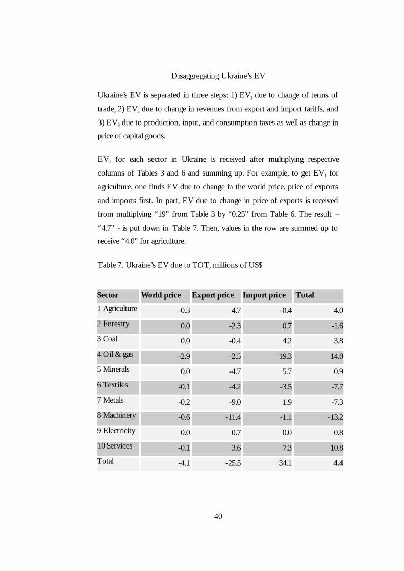
Disaggregating Ukraine’s EV

Ukraine’s EV is separated in three steps: 1) EV1 due to change of terms of

trade, 2) EV2 due to change in revenues from export and import tariffs, and

3) EV3 due to production, input, and consumption taxes as well as change in

price of capital goods.

EV1 for each sector in Ukraine is received after multiplying respective

columns of Tables 3 and 6 and summing up. For example, to get EV1 for

agriculture, one finds EV due to change in the world price, price of exports

and imports first. In part, EV due to change in price of exports is received

from multiplying “19” from Table 3 by “0.25” from Table 6. The result –

“4.7” - is put down in Table 7. Then, values in the row are summed up to

receive “4.0” for agriculture.

Table 7. Ukraine’s EV due to TOT, millions of US$

Sector World price Export price Import price Total

1 Agriculture -0.3 4.7 -0.4 4.0

2 Forestry 0.0 -2.3 0.7 -1.6

3 Coal 0.0 -0.4 4.2 3.8

4 Oil & gas -2.9 -2.5 19.3 14.0

5 Minerals 0.0 -4.7 5.7 0.9

6 Textiles -0.1 -4.2 -3.5 -7.7

7 Metals -0.2 -9.0 1.9 -7.3

8 Machinery -0.6 -11.4 -1.1 -13.2

9 Electricity 0.0 0.7 0.0 0.8

10 Services -0.1 3.6 7.3 10.8

Total -4.1 -25.5 34.1 4.4

41

EV due to change in TOT comprises $4.4mn for Ukraine. We can se that

despite negative figure for FSU (-$498mn) the number for Ukraine is positive.

This result is, mainly, due to small exports by Ukraine of forestry and oil &

gas.

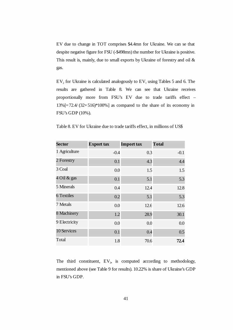
EV2 for Ukraine is calculated analogously to EV1 using Tables 5 and 6. The

results are gathered in Table 8. We can see that Ukraine receives

proportionally more from FSU’s EV due to trade tariffs effect –

13%[=72.4/(32+516)*100%] as compared to the share of its economy in

FSU’s GDP (10%).

Table 8. EV for Ukraine due to trade tariffs effect, in millions of US$

Sector Export tax Import tax Total

1 Agriculture -0.4 0.3 -0.1

2 Forestry 0.1 4.3 4.4

3 Coal 0.0 1.5 1.5

4 Oil & gas 0.1 5.1 5.3

5 Minerals 0.4 12.4 12.8

6 Textiles 0.2 5.1 5.3

7 Metals 0.0 12.6 12.6

8 Machinery 1.2 28.9 30.1

9 Electricity 0.0 0.0 0.0

10 Services 0.1 0.4 0.5

Total 1.8 70.6 72.4

The third constituent, EV3, is computed according to methodology,

mentioned above (see Table 9 for results). 10.22% is share of Ukraine’s GDP

in FSU’s GDP.

42

Table 9. Decomposition for Ukraine of EV due to capital goods as well as production, input and consumption tax, in millions of US$

Type of tax FSU Weighing, % Ukraine

Capital goods 104.6 10.22 10.7

Input tax 36.3 10.22 3.7

Production tax 38.0 10.22 3.9

Consumption tax -33.2 10.22 -3.4

Total 145.6 14.9

The final step is gathering all the figures together (Table 10). We see that

Ukraine gets about 47% of FSU’s EV (=91.7/195).

Table 10. Summing up EV for Ukraine, in millions of US$

TOT 4.4

Allocation, trade tariffs 72.4

The rest, proportional to GDP 14.9

Total 91.7

Comparing base and alternative scenarios

Calculations for alternative scenario are performed under the same

methodology as for base scenario. EV for Ukraine under alternative scenario

constitutes –$52.5 millions and for FSU the number is -$1182 millions. The

received numbers suggest that Ukraine would appropriate 4.44% [= (-52.5)/

(-1182)*100%] of FSU’s loss from joining CU with the EU if agricultural

sector were liberalized too. Negative figure for FSU comes from deterioration

43

in TOT for imported agricultural products. As Ukraine comprises 6% of total

FSU’s agricultural imports, it is hurt less. But still, it also faces deterioration in

export prices, which results in negative figure for Ukraine in general.

Proposals for future research

This research has a few weaknesses that free space for future research. The

first weakness is inconsistency of data on FSU in GTAP. Data on FSU’s trade

(IMF, 1998) used for disaggregation is higher than this in GTAP. As GTAP

data on FSU resembles the data provided by the WTO (2000), I can question

the quality of FSU trade data in GTAP. The reason for this is that WTO also

uses COMTRADE (COModity TRADE) data of the UN as GTAP does, but

there is a remark in WTO (2000) that the data for FSU includes intra-region

trade only starting from the year 1996. Version 4 of GTAP is composed for

the year 1995 and total FSU’s trade is argued to include intra-region trade.

Such explanation clarifies also inconsistency faced during disaggregation,

when Ukraine’s adjusted imports of oil & gas as well as coal exceeded the

respective figure for FSU (part of which Ukraine is). As Ukrainian imports of

fuel mostly come from Russia (intra-region trade), this number is not included

in inter-region trade (reported by WTO and supposedly used in GTAP).

Refining data on FSU or, due to the problem of lack of data for 1995, using

the next version of GTAP (forthcoming version 5 is composed for year 1997)

should make estimates more precise. Using version 5 would also eliminate the

shortcomings from Baltic States being part of FSU. They are represented

separately in version 5.

The second problem is availability of data on other states of FSU region.

GTAP allows disaggregating non-trade allocation effects (Table 9) on industry

basis. As input-output tables for other countries of FSU are not accumulated

in Derzhkomstat and it is rather specific information to be gathered by

international organizations, I made disaggregation proportionally to share of

44

Ukraine’s GDP in FSU’s GDP. This introduces inaccuracy into calculations

and can be treated by applying for data to State Statistical Committees of

respective states.

The next suggestion for research comes from absence of Ukraine as a

separate region in GTAP. Singling out Ukraine in the model and performing a

standard for GTAP procedure of data correction would refine the evaluation

considerably. This procedure would also allow simulating joining of Ukraine

alone to the EU, and not in the family of all FSU countries.

Further, the model assumes perfect competition and constant returns to scale,

while some authors (Rutherford and Tarr, 1998) contend that large group

monopolistic competition and IRTS should be used. Those claims could be

investigated and implemented in future research too.

Finally, static models underestimate consequences from trade liberalization

(Rutherford and Tarr, 1998). Thus, when dynamic model is publicly available,

it could be used for refining results received with this static model.

45

C h a p t e r 6

CONCLUSION

As the model predicts, Ukraine stands to gain from joining customs union

with the European Union if agricultural sector is excluded from agreement.

The respective gain – $91.7 millions – is to accrue yearly in terms of better

terms of trade (TOT), higher budget revenue from taxes gathered, and

appreciation in the value of investment goods. Ukraine’s gain constitutes 47%

of FSU’s equivalent variation, while its GDP comprises 10% and volume of

trade – 13% of respective indicators of FSU. This means Ukraine would gain

disproportionally more than on average other FSU countries under base

scenario.

The alternative scenario suggests that imitating EU’s highly protected

agricultural sector would be undesirable for Ukraine. It would worsen TOT in

import as well as export of agricultural products for Ukraine (EV makes up

-$101 and -$88 millions, respectively). Import prices would increase because

of elimination of 20% subsidy on export of agricultural products from EU

(on average) and higher common external tariffs (CET) in the EU on imports

from third countries. Export prices would decrease due to higher import

taxes of third countries on agricultural products from the EU (and its CU

partners) as response to EU’s protectionism.

Therefore, the final result is sensitive to shocks performed on tariffs to

agricultural products. The EU is considering slashing its export subsidies to

avoid difficulties with common agricultural policy after enlargement. Such

step will be followed by bilateral reducing tariffs with third countries in this

sector. Such modifications are expected to make Ukraine’s gain higher,

46

because it would benefit from expanding its exports to the EU and not lose

on the markets of third countries.

47

WORKS CITED

Baldwin, Richard E. and Rikard Forslid (1998). “Incremental Trade and Endogenous Growth: A q-Theory Approach”. NBER Working Paper # 6477. March.

Business Central Europe (2001). EBRD. Accessed May 2001 at: www.bcemag.com /statsdb/

Chang, Won, L. Allan Winters (1999). “How Regional Blocks Affect Excluded Countries. The Price Effects of MERCOSUR”. World Bank Working Paper # 2157. August.

Commission press release (2000). 29 November.

“Composite Paper. Reports on progress towards accession by each of the candidate countries “ (1999). European Commission. July.

Copenhagen European Council (1993). Presidency Conclusions. 21 and 22 June. Available at: http://www.europarl.eu.int/enlargement/ec/en/cop.htm

Cosgrove-Sacks, Carol (2000). “The role of the

Economic Commission for Europe” in Victoria Curzon Price, Alice Landau and Richard G. Whitman, ed. “The Enlargement of the European Union”.

Dixit, Avinash K., Joseph E. Stiglitz (1977). “Monopolistic Competition and Optimum Product Diversity”. The American Economic Review 67, pp.297-308. *

Doppelhofer, Gernot, Ronald I. Miller, and Xavier Sala-i-Martin (2000). “Determinants of Long-Term Growth: A Bayesian Averaging of Classical Estimates (BACE) Approach”. NBER Working Paper # 7750. June.

EU business (2000). 21 November, 29 November. Available at: www.eubusiness.com

EU/Ukraine Summit Vienna (1998). 16 October. Available at: http://www.eubusiness.com/easteuro/981015co.htm

European Commission (1998). Available at: www.newsroom.de/eu-kommission/themen/themen.cfm?main=white.htm&menu=er_link.htm

48

European Council Common Strategy on Ukraine (1999). December.

Franco, Mark (2000). “The enlargement: the European Commission’s viewpoint” in Victoria Curzon Price, Alice Landau and Richard G. Whitman, ed. “The Enlargement of the European Union”.

Geraci, Vincent J., Wilfried Prewo (1982). “An Empirical Demand and Supply Model of Multilateral Trade”. The Review of Economics and Statistics 64, pp.432-441. *

Hanoch, Giora (1975). “Production and Demand Models with Direct and Indirect Implicit Additivity”. Econometrica 43, pp. 395-420. May.

Harrison, Glenn W., Thomas F. Rutherford, and David G. Tarr (1996). “Economic Implications for Turkey of a Customs Union with the European Union”. World Bank Working Paper # 1599. May.

Helsinki European Council (1999). Presidency Conclusions. 10 and 11 December. Press Release: Brussels, No 00300/99. Available at: http://www.europarl.eu.int/enlargement/ec/en/hel.htm

Hertel, Thomas W., ed. (1997). “Global Trade Analysis: Modeling and Applications”. Cambridge University Press.

Hertel, Thomas W., ed. (2001). Lecture Notes to Internet Course of GTAP. Center for Global Trade Analysis. Purdue University. Available at: www.agecon.purdue.edu/gtap/courses

Hertel, Thomas W. and Marinos E. Tsigas (1997). “Structure of GTAP” as in Hertel, Thomas W. (1997). “Global Trade Analysis: Modeling and Applications”. Cambridge University Press.

Hoffmann, Lutz and Felicitas Moellers, ed. (2001). “Ukrayina na shlyakhu do Yevropy” (In Ukrainian - “Ukraine on the road to Europe”). “Fenix”.

Huff, Karen M., Kevin Hanslow, Thomas W. Hertel, and Marinos E. Tsigas (1997). “GTAP behavioral parameters” as in Hertel, Thomas W. (1997). “Global Trade Analysis: Modeling and Applications”. Cambridge University Press.

Howe, H. (1975). “Development of the Extended Linear Expenditure System from

49

Simple Savings Assumptions”. European Economic Review 6, pp. 305-310.

Institutions of the European Union (2000). Available at: http://europa.eu.int/inst-en.htm

IMF (1998). “Direction of Trade Statistics Yearbook”.

James, Barry (1999a). “Left out of EU, Ukraine Fears ‘Eurocurtain’ Isolation”. International Harold Tribune. Available at: http://www.iht.com/IHT/BJ/99/bj111299.html

----------------- (1999b). “Ukraine Doesn’t Take EU ‘No’ as Final”. The World’s Daily Newspaper. 20 December 1999.

“Joint Statement by the President of the European Council, J. Chirac assisted by the Secretary General of the Council/ High Representative for Common Foreign and Security Policy of the EU, J. Solana, the President of the Commission of the European Communities R. Prodi, and the President of Ukraine L. D. Kuchma” (2000). EU-Ukraine Summit. Paris. 15 September.

Kaufmann, Daniel (1997). "The Missing Pillar of a Growth Strategy for Ukraine: Institutional and Policy Reforms for Private Sector Development." HIID Development Discussion Paper #603. September.

Keller, W. J. (1980). “Tax Incidence: A General Equilibrium Approach”. Amsterdam. North Holand.

Kose, M. Ayahan and Raymond Riezman (2000). “Small Countries and Preferential Trade Agreements: How Severe is the Innocent Bystander Problem?”. CESifo Working Paper # 253. February.

Maastricht Treaty (1992). Heads of State of Government of countries of the EU. Accessed November 2000 at: www.ph.kcl.ac.uk/local /maas/protoco.txt

Michalopoulos, Constantine (1999). “The Integration of Transition Economies into the World Trading System”. World Bank Working Paper #2182. September.

Pakhomov, Y. M., D. G. Lukya-nenko, B. V. Hubskyi (1997). “Natsionalna ekonomika v hlobalnomu konkurentnomu ceredovyshchi” (In Ukrainian - “National

50

Economy in Global Competitive Environment”). “Ukrayina”. Kyiv.

Partnership and Co-operation Agreement between the European Communities and their Member States, and Ukraine (1994). 14 June.

Partridge, Ben (1999). “Ukraine: Minister Wants Positive Signal From EU On Membership”. RFE/RL. 3 February. Available at: http://www.rferl.org/nca/features/1999/02/F.RU.990203125905.HTML

Postup’s Infobank (2000). 11 October, 19 October, 2 November, 7 November.

Postup’s Infobank (2001). 17 January.

Price, Victoria Curzon and Alice Landau (2000). “The enlargement of the European Union: dealing with complexity” in Victoria Curzon Price, Alice Landau and Richard G. Whitman, ed. “The Enlargement of the European Union”.

Price, Victoria Curzon, Alice Landau and Richard G. Whitman, ed. (2000). “The Enlargement of the European Union”. Routledge.

Prodi, Romano (2000). President of the European Commission. Speech in Kiev, 10 November.

“Program of Ukraine’s integration into the EU” (2000). (In Ukrainian). #10-72 of 14 September.

Rivera-Batiz, L. and P. Romer (1991). “International Trade with Endogenous Technological Change”. European Economic Review 35, pp. 715-721.

Rodriguez, Francisco, Dani Rodrik (1999). “Trade Policy and Economic Growth: A Skeptic’s Guide to the Cross-National Evidence”. NBER Working Paper # 7081. Available at: http:// www.nber.org/papers/w7081

Rutherford, Thomas F, David G. Tarr (1998). “Trade Liberalization and Endogenous Growth in a Small Open Economy : A Quantitative Assessment”. World Bank Working Paper #1970. September.

Sala-i-Martin, Xavier X. (1997). “I Just Run Four Million Regressions”. NBER Working Paper # 6252. November.

Suranovic, Steven (1999). “International Trade

51

Theory and Policy Lecture Notes”. Accessed September 2000 at: inter nationalecon.com/test/

The Economist (1997). 20 December.

TSN (2001). News service on the channel “1 plus 1”. April 18.

Wacziarg, Romain (1998). “Measuring the Dynamic Gains from Trade”. World Bank Discussion Paper. Version from May.

World Bank (2001). World Bank Development Statistics. Available at: devdata.worldbank.org

WTO (2000). “Monitoring Country Progress in Central and Eastern Europe and Eurasia”. International Trade Statistics 2000. USAID/E&E/PCS. May.

52

APPENDIX A: AGGREGATION OF REGIONS

Definition of new (aggregated) regions

ase Quickly growing Asian economies (including China) and Japan

usa USA

eun European Union

eft EFTA

cea Central European Associates

fsu Former Soviet Union

tur Turkey

row Rest of the world

Regions mapping

Previous Previous region definition New

AUS Australia row

NZL New Zealand row

JPN Japan ase

KOR Republic of Korea ase

IDN Indonesia ase

MYS Malaysia ase

PHL Philippines ase

SGP Singapore ase

THA Thailand ase

VNM Viet Nam row

CHN China ase

HKG Hong Kong ase

TWN Taiwan ase

IND India row

LKA Sri Lanka row

53

RAS Rest of South Asia row

CAN Canada row

USA United States of America usa

MEX Mexico row

CAM Central America and Caribbean row

VEN Venezuela row

COL Colombia row

RAP Rest of Andean Pact row

ARG Argentina row

BRA Brazil row

CHL Chile row

URY Uruguay row

RSM Rest of South America row

GBR United Kingdom eun

DEU Germany eun

DNK Denmark eun

SWE Sweden eun

FIN Finland eun

REU Rest of European Union eun

EFT European Free Trade Area eft

CEA Central European Associates cea

FSU Former Soviet Union fsu

TUR Turkey tur

RME Rest of Middle East row

MAR Morocco row

RNF Rest of North Africa row

SAF South African Customs Union row

RSA Rest of Southern Africa row

RSS Rest of Sub Saharan Africa row

ROW Rest of World row

54

APPENDIX B: AGGREGATION OF INDUSTRIES

Definition of new (aggregated) sectors

1. agr Food products, plant-based fibers, fishery, beverages and

tobacco

2. for Forestry, wood and paper products

3. col Coal

4. o_g Oil, gas, petroleum and coal products

5. min Minerals and chemicals

6. tex Textiles, wearing apparels, and leather products

7. fer Metals and metal products

8. mac Motor vehicles, transport and electronic equipment, machinery

9. ele Electricity

10. ser Utilities, trade, transport, construction, financial services

Industries mapping

Previous Previous industry definition New

1. pdr Paddy rice agr

2. wht Wheat agr

3. gro Other cereal grains agr

4. v_f Vegetables, fruit, nuts agr

5. osd Oil seeds agr

6. c_b Sugar cane, sugar beet agr

7. pfb Plant-based fibers agr

8. ocr Other crops agr

9. ctl Bovine cattle, sheep and goats, horses agr

10. oap Other animal products agr

55

11. rmk Raw milk agr

12. wol Wool silk-worm cocoons agr

13. for Forestry for

14. fsh Fishing agr

15. col Coal col

16. oil Oil o_g

17. gas Gas o_g

18. omn Other minerals min

19. cmt Bovine cattle, sheep and goat, horse meat prods agr

20. omt Other meat products agr

21. vol Vegetable oils and fats agr

22. mil Dairy products agr

23. pcr Processed rice agr

24. sgr Sugar agr

25. ofd Other food products agr

26. b_t Beverages and tobacco products agr

27. tex Textiles tex

28. wap Wearing apparel tex

29. lea Leather products tex

30. lum Wood products for

31. ppp Paper products, publishing for

32. p_c Petroleum, coal products o_g

33. crp Chemical, rubber, plastic products min

34. nmm Other mineral products min

35. i_s Ferrous metals fer

36. nfm Other metals fer

37. fmp Metal products fer

38. mvh Motor vehicles and parts mac

39. otn Other transport equipment mac

40. ele Electronic equipment mac

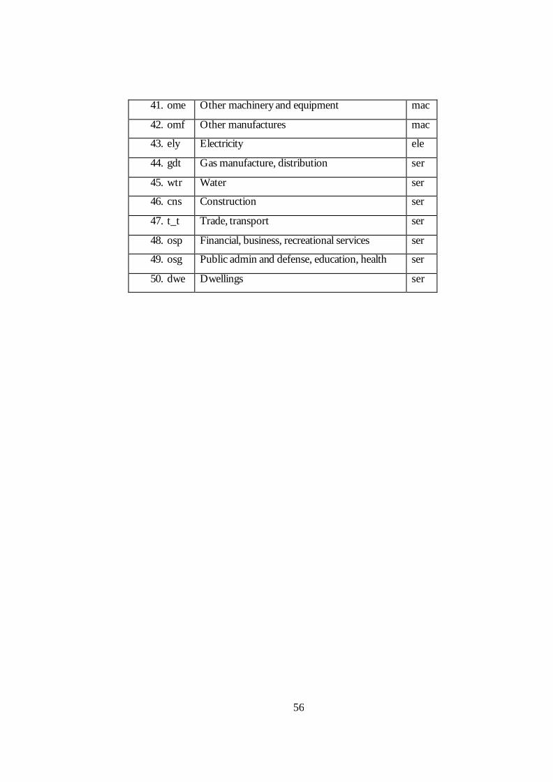
56

41. ome Other machinery and equipment mac

42. omf Other manufactures mac

43. ely Electricity ele

44. gdt Gas manufacture, distribution ser

45. wtr Water ser

46. cns Construction ser

47. t_t Trade, transport ser

48. osp Financial, business, recreational services ser

49. osg Public admin and defense, education, health ser

50. dwe Dwellings ser

57

APPENDIX C: SHOCKS PERFORMED UNDER THE FIRST

SIMULATION (BASE SCENARIO)

Shock tms("for","eun","tur") = -4.74 - change in power of import tariff on forestry delivered from the EU to Turkey, levied in Turkey Shock txs("ele","cea","eun") = -0.76 - change in the power of export tariff on electricity delivered from CEA to the EU, levied in CEA ! Sim 1d: CEEC&Turkey(-agr) join the EU/ form CU with it + adj! !CEEC eliminate tariffs in itself! Shock tms("agr","cea","cea") = -10.79; Shock tms("for","cea","cea") = -3.97; Shock tms("col","cea","cea") = -2.89; Shock tms("o_g","cea","cea") = -4.66; Shock tms("min","cea","cea") = -6.09; Shock tms("tex","cea","cea") = -9.60; Shock tms("fer","cea","cea") = -4.43; Shock tms("mac","cea","cea") = -7.46; Shock txs("agr","cea","cea") = -2.35; Shock txs("mac","cea","cea") = -0.05; Shock txs("ele","cea","cea") = -0.76; ! The EU eliminates bilateral tariffs with CEEC! Shock tms("agr","cea","eun") = -22.32; Shock tms("for","cea","eun") = -2.59; Shock tms("o_g","cea","eun") = -1.69; Shock tms("min","cea","eun") = -3.06; Shock tms("tex","cea","eun") = -6.23; Shock tms("fer","cea","eun") = -3.40; Shock tms("mac","cea","eun") = -3.86; Shock tms("ser","cea","eun") = -0.02; Shock txs("agr","eun","cea") = -11.16; Shock txs("for","eun","cea") = 0.34; Shock txs("col","eun","cea") = 0.53; Shock txs("o_g","eun","cea") = 0.59; Shock txs("min","eun","cea") = 0.49; Shock txs("tex","eun","cea") = 0.46; Shock txs("fer","eun","cea") = 0.39; Shock txs("mac","eun","cea") = 0.38; Shock txs("ele","eun","cea") = 0.65; Shock txs("ser","eun","cea") = 0.81; !CEEC eliminates bilateral tariffs with the EU! Shock tms("agr","eun","cea") = -14.06; Shock tms("for","eun","cea") = -5.92; Shock tms("col","eun","cea") = -4.74; Shock tms("o_g","eun","cea") = -6.34; Shock tms("min","eun","cea") = -7.68; Shock tms("tex","eun","cea") = -8.39; Shock tms("fer","eun","cea") = -5.97; Shock tms("mac","eun","cea") = -7.21; Shock txs("agr","cea","eun") = -8.54; Shock txs("tex","cea","eun") = 0.01; Shock txs("mac","cea","eun") = -0.06; Shock txs("ele","cea","eun") = -0.76; !Turkey eliminates bilateral tariffs with the EU!

Shock tms("for","eun","tur") = -4.74; Shock tms("col","eun","tur") = -1.22; Shock tms("o_g","eun","tur") = -12.94; Shock tms("min","eun","tur") = -4.56; Shock tms("tex","eun","tur") = -6.37; Shock tms("fer","eun","tur") = -4.15; Shock tms("mac","eun","tur") = -4.36; Shock txs("for","tur","eun") = -0.10; Shock txs("col","tur","eun") = -27.42; Shock txs("o_g","tur","eun") = -7.29; Shock txs("min","tur","eun") = -3.72; Shock txs("tex","tur","eun") = 0.03; Shock txs("mac","tur","eun") = -0.08; !The EU eliminates bilateral tariffs with Turkey! Shock tms("for","tur","eun") = -2.61; Shock tms("col","tur","eun") = -0.60; Shock tms("o_g","tur","eun") = -1.40; Shock tms("min","tur","eun") = -3.61; Shock tms("tex","tur","eun") = -8.30; Shock tms("fer","tur","eun") = -3.44; Shock tms("mac","tur","eun") = -4.47; Shock tms("ser","tur","eun") = -0.01; Shock txs("for","eun","tur") = 0.42; Shock txs("col","eun","tur") = 0.82; Shock txs("o_g","eun","tur") = 1.04; Shock txs("min","eun","tur") = 0.58; Shock txs("tex","eun","tur") = 0.58; Shock txs("fer","eun","tur") = 0.61; Shock txs("mac","eun","tur") = 0.40; Shock txs("ser","eun","tur") = 0.75; !Turkey eliminates bilateral tariffs with CEEC! Shock tms("agr","cea","tur") =18.04 ; Shock tms("for","cea","tur") = -7.12; Shock tms("col","cea","tur") = -1.35; Shock tms("o_g","cea","tur") = -17.53; Shock tms("min","cea","tur") = -8.42; Shock tms("tex","cea","tur") = -8.89; Shock tms("fer","cea","tur") = -4.66; Shock tms("mac","cea","tur") = -9.10; Shock txs("agr","tur","cea") = 2.19; Shock txs("for","tur","cea") = -0.11; Shock txs("col","tur","cea") = -27.42; Shock txs("o_g","tur","cea") = -37.64; Shock txs("min","tur","cea") = -2.24; Shock txs("mac","tur","cea") = -0.08; !CEEC eliminate bilateral tariffs with Turkey! Shock tms("agr","tur","cea") = -8.33;

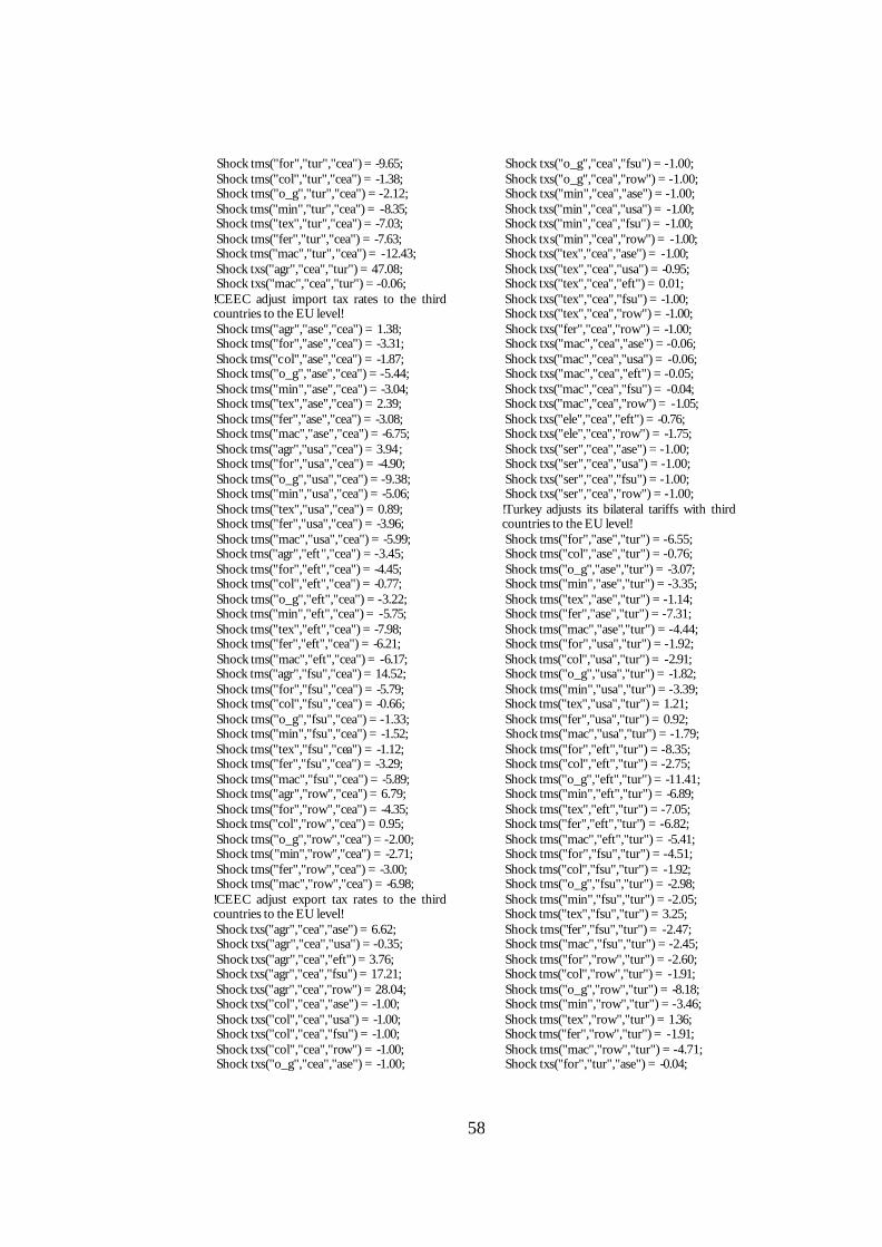
58

Shock tms("for","tur","cea") = -9.65; Shock tms("col","tur","cea") = -1.38; Shock tms("o_g","tur","cea") = -2.12; Shock tms("min","tur","cea") = -8.35; Shock tms("tex","tur","cea") = -7.03; Shock tms("fer","tur","cea") = -7.63; Shock tms("mac","tur","cea") = -12.43; Shock txs("agr","cea","tur") = 47.08; Shock txs("mac","cea","tur") = -0.06; !CEEC adjust import tax rates to the third countries to the EU level! Shock tms("agr","ase","cea") = 1.38; Shock tms("for","ase","cea") = -3.31; Shock tms("col","ase","cea") = -1.87; Shock tms("o_g","ase","cea") = -5.44; Shock tms("min","ase","cea") = -3.04; Shock tms("tex","ase","cea") = 2.39; Shock tms("fer","ase","cea") = -3.08; Shock tms("mac","ase","cea") = -6.75; Shock tms("agr","usa","cea") = 3.94; Shock tms("for","usa","cea") = -4.90; Shock tms("o_g","usa","cea") = -9.38; Shock tms("min","usa","cea") = -5.06; Shock tms("tex","usa","cea") = 0.89; Shock tms("fer","usa","cea") = -3.96; Shock tms("mac","usa","cea") = -5.99; Shock tms("agr","eft","cea") = -3.45; Shock tms("for","eft","cea") = -4.45; Shock tms("col","eft","cea") = -0.77; Shock tms("o_g","eft","cea") = -3.22; Shock tms("min","eft","cea") = -5.75; Shock tms("tex","eft","cea") = -7.98; Shock tms("fer","eft","cea") = -6.21; Shock tms("mac","eft","cea") = -6.17; Shock tms("agr","fsu","cea") = 14.52; Shock tms("for","fsu","cea") = -5.79; Shock tms("col","fsu","cea") = -0.66; Shock tms("o_g","fsu","cea") = -1.33; Shock tms("min","fsu","cea") = -1.52; Shock tms("tex","fsu","cea") = -1.12; Shock tms("fer","fsu","cea") = -3.29; Shock tms("mac","fsu","cea") = -5.89; Shock tms("agr","row","cea") = 6.79; Shock tms("for","row","cea") = -4.35; Shock tms("col","row","cea") = 0.95; Shock tms("o_g","row","cea") = -2.00; Shock tms("min","row","cea") = -2.71; Shock tms("fer","row","cea") = -3.00; Shock tms("mac","row","cea") = -6.98; !CEEC adjust export tax rates to the third countries to the EU level! Shock txs("agr","cea","ase") = 6.62; Shock txs("agr","cea","usa") = -0.35; Shock txs("agr","cea","eft") = 3.76; Shock txs("agr","cea","fsu") = 17.21; Shock txs("agr","cea","row") = 28.04; Shock txs("col","cea","ase") = -1.00; Shock txs("col","cea","usa") = -1.00; Shock txs("col","cea","fsu") = -1.00; Shock txs("col","cea","row") = -1.00; Shock txs("o_g","cea","ase") = -1.00;

Shock txs("o_g","cea","fsu") = -1.00; Shock txs("o_g","cea","row") = -1.00; Shock txs("min","cea","ase") = -1.00; Shock txs("min","cea","usa") = -1.00; Shock txs("min","cea","fsu") = -1.00; Shock txs("min","cea","row") = -1.00; Shock txs("tex","cea","ase") = -1.00; Shock txs("tex","cea","usa") = -0.95; Shock txs("tex","cea","eft") = 0.01; Shock txs("tex","cea","fsu") = -1.00; Shock txs("tex","cea","row") = -1.00; Shock txs("fer","cea","row") = -1.00; Shock txs("mac","cea","ase") = -0.06; Shock txs("mac","cea","usa") = -0.06; Shock txs("mac","cea","eft") = -0.05; Shock txs("mac","cea","fsu") = -0.04; Shock txs("mac","cea","row") = -1.05; Shock txs("ele","cea","eft") = -0.76; Shock txs("ele","cea","row") = -1.75; Shock txs("ser","cea","ase") = -1.00; Shock txs("ser","cea","usa") = -1.00; Shock txs("ser","cea","fsu") = -1.00; Shock txs("ser","cea","row") = -1.00; !Turkey adjusts its bilateral tariffs with third countries to the EU level! Shock tms("for","ase","tur") = -6.55; Shock tms("col","ase","tur") = -0.76; Shock tms("o_g","ase","tur") = -3.07; Shock tms("min","ase","tur") = -3.35; Shock tms("tex","ase","tur") = -1.14; Shock tms("fer","ase","tur") = -7.31; Shock tms("mac","ase","tur") = -4.44; Shock tms("for","usa","tur") = -1.92; Shock tms("col","usa","tur") = -2.91; Shock tms("o_g","usa","tur") = -1.82; Shock tms("min","usa","tur") = -3.39; Shock tms("tex","usa","tur") = 1.21; Shock tms("fer","usa","tur") = 0.92; Shock tms("mac","usa","tur") = -1.79; Shock tms("for","eft","tur") = -8.35; Shock tms("col","eft","tur") = -2.75; Shock tms("o_g","eft","tur") = -11.41; Shock tms("min","eft","tur") = -6.89; Shock tms("tex","eft","tur") = -7.05; Shock tms("fer","eft","tur") = -6.82; Shock tms("mac","eft","tur") = -5.41; Shock tms("for","fsu","tur") = -4.51; Shock tms("col","fsu","tur") = -1.92; Shock tms("o_g","fsu","tur") = -2.98; Shock tms("min","fsu","tur") = -2.05; Shock tms("tex","fsu","tur") = 3.25; Shock tms("fer","fsu","tur") = -2.47; Shock tms("mac","fsu","tur") = -2.45; Shock tms("for","row","tur") = -2.60; Shock tms("col","row","tur") = -1.91; Shock tms("o_g","row","tur") = -8.18; Shock tms("min","row","tur") = -3.46; Shock tms("tex","row","tur") = 1.36; Shock tms("fer","row","tur") = -1.91; Shock tms("mac","row","tur") = -4.71; Shock txs("for","tur","ase") = -0.04;

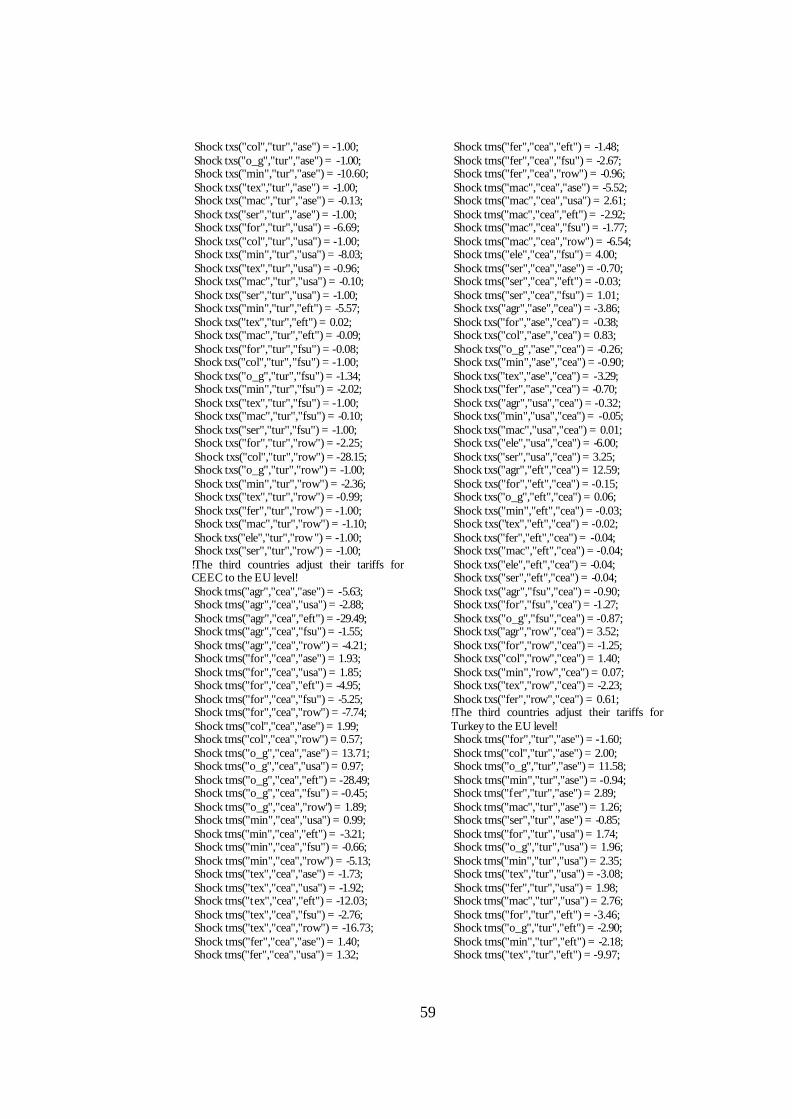
59

Shock txs("col","tur","ase") = -1.00; Shock txs("o_g","tur","ase") = -1.00; Shock txs("min","tur","ase") = -10.60; Shock txs("tex","tur","ase") = -1.00; Shock txs("mac","tur","ase") = -0.13; Shock txs("ser","tur","ase") = -1.00; Shock txs("for","tur","usa") = -6.69; Shock txs("col","tur","usa") = -1.00; Shock txs("min","tur","usa") = -8.03; Shock txs("tex","tur","usa") = -0.96; Shock txs("mac","tur","usa") = -0.10; Shock txs("ser","tur","usa") = -1.00; Shock txs("min","tur","eft") = -5.57; Shock txs("tex","tur","eft") = 0.02; Shock txs("mac","tur","eft") = -0.09; Shock txs("for","tur","fsu") = -0.08; Shock txs("col","tur","fsu") = -1.00; Shock txs("o_g","tur","fsu") = -1.34; Shock txs("min","tur","fsu") = -2.02; Shock txs("tex","tur","fsu") = -1.00; Shock txs("mac","tur","fsu") = -0.10; Shock txs("ser","tur","fsu") = -1.00; Shock txs("for","tur","row") = -2.25; Shock txs("col","tur","row") = -28.15; Shock txs("o_g","tur","row") = -1.00; Shock txs("min","tur","row") = -2.36; Shock txs("tex","tur","row") = -0.99; Shock txs("fer","tur","row") = -1.00; Shock txs("mac","tur","row") = -1.10; Shock txs("ele","tur","row ") = -1.00; Shock txs("ser","tur","row") = -1.00; !The third countries adjust their tariffs for CEEC to the EU level! Shock tms("agr","cea","ase") = -5.63; Shock tms("agr","cea","usa") = -2.88; Shock tms("agr","cea","eft") = -29.49; Shock tms("agr","cea","fsu") = -1.55; Shock tms("agr","cea","row") = -4.21; Shock tms("for","cea","ase") = 1.93; Shock tms("for","cea","usa") = 1.85; Shock tms("for","cea","eft") = -4.95; Shock tms("for","cea","fsu") = -5.25; Shock tms("for","cea","row") = -7.74; Shock tms("col","cea","ase") = 1.99; Shock tms("col","cea","row") = 0.57; Shock tms("o_g","cea","ase") = 13.71; Shock tms("o_g","cea","usa") = 0.97; Shock tms("o_g","cea","eft") = -28.49; Shock tms("o_g","cea","fsu") = -0.45; Shock tms("o_g","cea","row") = 1.89; Shock tms("min","cea","usa") = 0.99; Shock tms("min","cea","eft") = -3.21; Shock tms("min","cea","fsu") = -0.66; Shock tms("min","cea","row") = -5.13; Shock tms("tex","cea","ase") = -1.73; Shock tms("tex","cea","usa") = -1.92; Shock tms("tex","cea","eft") = -12.03; Shock tms("tex","cea","fsu") = -2.76; Shock tms("tex","cea","row") = -16.73; Shock tms("fer","cea","ase") = 1.40; Shock tms("fer","cea","usa") = 1.32;

Shock tms("fer","cea","eft") = -1.48; Shock tms("fer","cea","fsu") = -2.67; Shock tms("fer","cea","row") = -0.96; Shock tms("mac","cea","ase") = -5.52; Shock tms("mac","cea","usa") = 2.61; Shock tms("mac","cea","eft") = -2.92; Shock tms("mac","cea","fsu") = -1.77; Shock tms("mac","cea","row") = -6.54; Shock tms("ele","cea","fsu") = 4.00; Shock tms("ser","cea","ase") = -0.70; Shock tms("ser","cea","eft") = -0.03; Shock tms("ser","cea","fsu") = 1.01; Shock txs("agr","ase","cea") = -3.86; Shock txs("for","ase","cea") = -0.38; Shock txs("col","ase","cea") = 0.83; Shock txs("o_g","ase","cea") = -0.26; Shock txs("min","ase","cea") = -0.90; Shock txs("tex","ase","cea") = -3.29; Shock txs("fer","ase","cea") = -0.70; Shock txs("agr","usa","cea") = -0.32; Shock txs("min","usa","cea") = -0.05; Shock txs("mac","usa","cea") = 0.01; Shock txs("ele","usa","cea") = -6.00; Shock txs("ser","usa","cea") = 3.25; Shock txs("agr","eft","cea") = 12.59; Shock txs("for","eft","cea") = -0.15; Shock txs("o_g","eft","cea") = 0.06; Shock txs("min","eft","cea") = -0.03; Shock txs("tex","eft","cea") = -0.02; Shock txs("fer","eft","cea") = -0.04; Shock txs("mac","eft","cea") = -0.04; Shock txs("ele","eft","cea") = -0.04; Shock txs("ser","eft","cea") = -0.04; Shock txs("agr","fsu","cea") = -0.90; Shock txs("for","fsu","cea") = -1.27; Shock txs("o_g","fsu","cea") = -0.87; Shock txs("agr","row","cea") = 3.52; Shock txs("for","row","cea") = -1.25; Shock txs("col","row","cea") = 1.40; Shock txs("min","row","cea") = 0.07; Shock txs("tex","row","cea") = -2.23; Shock txs("fer","row","cea") = 0.61; !The third countries adjust their tariffs for Turkey to the EU level! Shock tms("for","tur","ase") = -1.60; Shock tms("col","tur","ase") = 2.00; Shock tms("o_g","tur","ase") = 11.58; Shock tms("min","tur","ase") = -0.94; Shock tms("fer","tur","ase") = 2.89; Shock tms("mac","tur","ase") = 1.26; Shock tms("ser","tur","ase") = -0.85; Shock tms("for","tur","usa") = 1.74; Shock tms("o_g","tur","usa") = 1.96; Shock tms("min","tur","usa") = 2.35; Shock tms("tex","tur","usa") = -3.08; Shock tms("fer","tur","usa") = 1.98; Shock tms("mac","tur","usa") = 2.76; Shock tms("for","tur","eft") = -3.46; Shock tms("o_g","tur","eft") = -2.90; Shock tms("min","tur","eft") = -2.18; Shock tms("tex","tur","eft") = -9.97;

60

Shock tms("fer","tur","eft") = -2.02; Shock tms("mac","tur","eft") = -1.93; Shock tms("ser","tur","eft") = -0.03; Shock tms("for","tur","fsu") = -5.83; Shock tms("col","tur","fsu") = 5.00; Shock tms("o_g","tur","fsu") = -7.15; Shock tms("min","tur","fsu") = -4.74; Shock tms("tex","tur","fsu") = -3.72; Shock tms("fer","tur","fsu") = -3.70; Shock tms("mac","tur","fsu") = -6.24; Shock tms("ele","tur","fsu") = 4.00; Shock tms("for","tur","row") = -4.98; Shock tms("col","tur","row") = -7.88; Shock tms("o_g","tur","row") = -2.66; Shock tms("min","tur","row") = -3.39; Shock tms("tex","tur","row") = 3.22; Shock tms("fer","tur","row") = 2.86; Shock tms("mac","tur","row") = -7.87; Shock tms("ele","tur","row") = 0.82; Shock txs("for","ase","tur") = 0.18; Shock txs("col","ase","tur") = -1.14; Shock txs("o_g","ase","tur") = -2.54; Shock txs("min","ase","tur") = -0.31; Shock txs("tex","ase","tur") = -4.96; Shock txs("fer","ase","tur") = 0.53;

Shock txs("mac","ase","tur") = -1.45; Shock txs("ser","ase","tur") = 0.29; Shock txs("o_g","usa","tur") = 0.01; Shock txs("min","usa","tur") = -0.06; Shock txs("fer","usa","tur") = 0.41; Shock txs("ele","usa","tur") = -6.00; Shock txs("ser","usa","tur") = 3.46; Shock txs("for","eft","tur") = -0.15; Shock txs("o_g","eft","tur") = 0.36; Shock txs("min","eft","tur") = -0.03; Shock txs("tex","eft","tur") = -0.02; Shock txs("fer","eft","tur") = -0.06; Shock txs("mac","eft","tur") = -0.04; Shock txs("ser","eft","tur") = -0.04; Shock txs("for","fsu","tur") = -1.41; Shock txs("o_g","fsu","tur") = -1.03; Shock txs("ele","fsu","tur") = 1.00; Shock txs("ser","fsu","tur") = -0.80; Shock txs("for","row","tur") = 0.69; Shock txs("o_g","row","tur") = -1.33; Shock txs("min","row","tur") = 0.22; Shock txs("tex","row","tur") = -1.94; Shock txs("fer","row","tur") = 0.25; Shock txs("ser","row","tur") = 0.18;

61

APPENDIX D: SHOCKS PERFORMED UNDER THE SECOND

SIMULATION (BASE SCENARIO)

Shock tms("for","eun","fsu") = -9.91 - change in power of import tariff on forestry delivered from the EU to FSU, levied in FSU Shock txs("agr","fsu","eun") = 1.83 - change in the power of export tariff on electricity delivered from FSU to the EU, levied in FSU ! Sim2d: FSU joins the EU (AA, --agr)! !FSU eliminates tariffs in itself! Shock tms("for","fsu","fsu") = -12.05; Shock tms("col","fsu","fsu") = -4.76; Shock tms("o_g","fsu","fsu") = -4.79; Shock tms("min","fsu","fsu") = -9.80; Shock tms("tex","fsu","fsu") = -12.90; Shock tms("fer","fsu","fsu") = -11.42; Shock tms("mac","fsu","fsu") = -8.98; Shock tms("ele","fsu","fsu") = -3.66; Shock tms("ser","fsu","fsu") = -1.75; Shock txs("for","fsu","fsu") = 0.58; Shock txs("col","fsu","fsu") = 1.05; Shock txs("o_g","fsu","fsu") = 3.18; Shock txs("min","fsu","fsu") = 0.32; Shock txs("tex","fsu","fsu") = 0.18; Shock txs("fer","fsu","fsu") = 0.19; Shock txs("mac","fsu","fsu") = 0.25; Shock txs("ele","fsu","fsu") = -0.72; Shock txs("ser","fsu","fsu") = 1.05; !The EU eliminates bilateral tariffs with FSU! Shock tms("for","fsu","eun") = -1.25; Shock tms("col","fsu","eun") = -0.50; Shock tms("o_g","fsu","eun") = -0.20; Shock tms("min","fsu","eun") = -3.85; Shock tms("tex","fsu","eun") = -7.37; Shock tms("fer","fsu","eun") = -2.12; Shock tms("mac","fsu","eun") = -4.42; Shock tms("ele","fsu","eun") = -0.10; Shock tms("ser","fsu","eun") = -0.03; Shock txs("for","eun","fsu") = 0.38; Shock txs("col","eun","fsu") = 1.04; Shock txs("o_g","eun","fsu") = 0.53; Shock txs("min","eun","fsu") = 0.45; Shock txs("tex","eun","fsu") = 0.52; Shock txs("fer","eun","fsu") = 0.37; Shock txs("mac","eun","fsu") = 0.31; Shock txs("ser","eun","fsu") = 0.78; !FSU eliminates bilateral tariffs with the EU! Shock tms("for","eun","fsu") = -9.91; Shock tms("col","eun","fsu") = -4.61; Shock tms("o_g","eun","fsu") = -4.77; Shock tms("min","eun","fsu") = -9.49; Shock tms("tex","eun","fsu") = -12.47; Shock tms("fer","eun","fsu") = -10.86; Shock tms("mac","eun","fsu") = -7.79; Shock tms("ele","eun","fsu") = -3.66; Shock tms("ser","eun","fsu") = -1.74;

Shock txs("for","fsu","eun") = 1.54; Shock txs("col","fsu","eun") = 1.05; Shock txs("o_g","fsu","eun") = 2.85; Shock txs("min","fsu","eun") = 0.37; Shock txs("tex","fsu","eun") = 0.15; Shock txs("fer","fsu","eun") = 0.25; Shock txs("mac","fsu","eun") = 0.27; Shock txs("ele","fsu","eun") = -0.72; Shock txs("ser","fsu","eun") = 0.61; !FSU eliminates bilateral tariffs with CEEC! Shock tms("for","cea","fsu") = -9.91; Shock tms("col","cea","fsu") = -4.76; Shock tms("o_g","cea","fsu") = -4.77; Shock tms("min","cea","fsu") = -9.91; Shock tms("tex","cea","fsu") = -12.28; Shock tms("fer","cea","fsu") = -10.71; Shock tms("mac","cea","fsu") = -8.25; Shock tms("ser","cea","fsu") = -1.96; Shock txs("for","fsu","cea") = 2.04; Shock txs("col","fsu","cea") = 1.05; Shock txs("o_g","fsu","cea") = 3.09; Shock txs("min","fsu","cea") = 0.41; Shock txs("tex","fsu","cea") = 0.19; Shock txs("fer","fsu","cea") = 0.23; Shock txs("mac","fsu","cea") = 0.31; Shock txs("ele","fsu","cea") = -0.72; Shock txs("ser","fsu","cea") = 0.75; !CEEC eliminate bilateral tariffs with FSU! Shock tms("for","fsu","cea") = -0.99; Shock tms("col","fsu","cea") = -0.99; Shock tms("min","fsu","cea") = -3.85; Shock tms("tex","fsu","cea") = -7.41; Shock tms("fer","fsu","cea") = -1.96; Shock tms("mac","fsu","cea") = -4.77; Shock txs("col","cea","fsu") = 1.01; Shock txs("o_g","cea","fsu") = 1.01; Shock txs("min","cea","fsu") = 1.01; Shock txs("tex","cea","fsu") = 1.01; Shock txs("ser","cea","fsu") = 1.01; !FSU eliminates bilateral tariffs w ith Turkey! Shock tms("for","tur","fsu") = -9.91; Shock tms("o_g","tur","fsu") = -4.77; Shock tms("min","tur","fsu") = -9.91; Shock tms("tex","tur","fsu") = -12.28; Shock tms("fer","tur","fsu") = -10.72; Shock tms("mac","tur","fsu") = -8.26; Shock tms("ser","tur","fsu") = -1.72; Shock txs("for","fsu","tur") = 2.04;

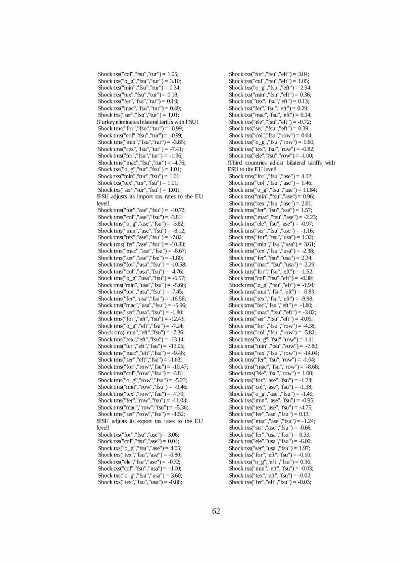
62

Shock txs("col","fsu","tur") = 1.05; Shock txs("o_g","fsu","tur") = 3.10; Shock txs("min","fsu","tur") = 0.34; Shock txs("tex","fsu","tur") = 0.18; Shock txs("fer","fsu","tur") = 0.19; Shock txs("mac","fsu","tur") = 0.49; Shock txs("ser","fsu","tur") = 1.01; !Turkey eliminates bilateral tariffs with FSU! Shock tms("for","fsu","tur") = -0.99; Shock tms("col","fsu","tur") = -0.99; Shock tms("min","fsu","tur") = -3.85; Shock tms("tex","fsu","tur") = -7.41; Shock tms("fer","fsu","tur") = -1.96; Shock tms("mac","fsu","tur") = -4.76; Shock txs("o_g","tur","fsu") = 1.01; Shock txs("min","tur","fsu") = 1.01; Shock txs("tex","tur","fsu") = 1.01; Shock txs("ser","tur","fsu") = 1.01; !FSU adjusts its import tax rates to the EU level! Shock tms("for","ase","fsu") = -10.72; Shock tms("col","ase","fsu") = -3.81; Shock tms("o_g","ase","fsu") = -3.82; Shock tms("min","ase","fsu") = -8.12; Shock tms("tex","ase","fsu") = -7.82; Shock tms("fer","ase","fsu") = -10.83; Shock tms("mac","ase","fsu") = -8.67; Shock tms("ser","ase","fsu") = -1.80; Shock tms("for","usa","fsu") = -10.58; Shock tms("col","usa","fsu") = -4.76; Shock tms("o_g","usa","fsu") = -6.57; Shock tms("min","usa","fsu") = -5.66; Shock tms("tex","usa","fsu") = -7.45; Shock tms("fer","usa","fsu") = -16.58; Shock tms("mac","usa","fsu") = -5.96; Shock tms("ser","usa","fsu") = -1.80; Shock tms("for","eft","fsu") = -12.43; Shock tms("o_g","eft","fsu") = -7.24; Shock tms("min","eft","fsu") = -7.36; Shock tms("tex","eft","fsu") = -13.14; Shock tms("fer","eft","fsu") = -13.05; Shock tms("mac","eft","fsu") = -9.46; Shock tms("ser","eft","fsu") = -1.63; Shock tms("for","row","fsu") = -10.47; Shock tms("col","row","fsu") = -3.81; Shock tms("o_g","row","fsu") = -5.23; Shock tms("min","row","fsu") = -9.46; Shock tms("tex","row","fsu") = -7.79; Shock tms("fer","row","fsu") = -11.03; Shock tms("mac","row","fsu") = -5.36; Shock tms("ser","row","fsu") = -1.52; !FSU adjusts its export tax rates to the EU level! Shock txs("for","fsu","ase") = 3.06; Shock txs("col","fsu","ase") = 0.04; Shock txs("o_g","fsu","ase") = 4.05; Shock txs("tex","fsu","ase") = -0.80; Shock txs("ele","fsu","ase") = -0.72; Shock txs("col","fsu","usa") = -1.00; Shock txs("o_g","fsu","usa") = 3.60; Shock txs("tex","fsu","usa") = -0.88;

Shock txs("for","fsu","eft") = 3.04; Shock txs("col","fsu","eft") = 1.05; Shock txs("o_g","fsu","eft") = 2.54; Shock txs("min","fsu","eft") = 0.36; Shock txs("tex","fsu","eft") = 0.13; Shock txs("fer","fsu","eft") = 0.29; Shock txs("mac","fsu","eft") = 0.34; Shock txs("ele","fsu","eft") = -0.72; Shock txs("ser","fsu","eft") = 0.39; Shock txs("col","fsu","row") = 0.04; Shock txs("o_g","fsu","row") = 1.60; Shock txs("tex","fsu","row") = -0.82; Shock txs("ele","fsu","row") = -1.00; !Third countries adjust bilateral tariffs with FSU to the EU level! Shock tms("for","fsu","ase") = 4.12; Shock tms("col","fsu","ase") = 1.46; Shock tms("o_g","fsu","ase") = 11.84; Shock tms("min","fsu","ase") = 0.96; Shock tms("tex","fsu","ase") = 2.01; Shock tms("fer","fsu","ase") = 1.57; Shock tms("mac","fsu","ase") = -2.23; Shock tms("ele","fsu","ase") = -0.97; Shock tms("ser","fsu","ase") = -1.16; Shock tms("for","fsu","usa") = 1.32; Shock tms("min","fsu","usa") = 3.61; Shock tms("tex","fsu","usa") = -2.38; Shock tms("fer","fsu","usa") = 2.34; Shock tms("mac","fsu","usa") = 2.29; Shock tms("for","fsu","eft") = -1.52; Shock tms("col","fsu","eft") = -0.30; Shock tms("o_g","fsu","eft") = -1.94; Shock tms("min","fsu","eft") = -0.83; Shock tms("tex","fsu","eft") = -9.98; Shock tms("fer","fsu","eft") = -1.80; Shock tms("mac","fsu","eft") = -3.82; Shock tms("ser","fsu","eft") = -0.05; Shock tms("for","fsu","row") = -4.38; Shock tms("col","fsu","row") = -5.82; Shock tms("o_g","fsu","row") = 1.11; Shock tms("min","fsu","row") = -7.80; Shock tms("tex","fsu","row") = -14.04; Shock tms("fer","fsu","row") = -1.04; Shock tms("mac","fsu","row") = -8.68; Shock tms("ele","fsu","row") = 1.00; Shock txs("for","ase","fsu") = -1.24; Shock txs("col","ase","fsu") = -1.38; Shock txs("o_g","ase","fsu") = -1.49; Shock txs("min","ase","fsu") = -0.95; Shock txs("tex","ase","fsu") = -4.75; Shock txs("fer","ase","fsu") = 0.13; Shock txs("mac","ase","fsu") = -1.24; Shock txs("ser","ase","fsu") = -0.66; Shock txs("fer","usa","fsu") = 0.33; Shock txs("ele","usa","fsu") = -6.00; Shock txs("ser","usa","fsu") = 1.97; Shock txs("for","eft","fsu") = -0.10; Shock txs("o_g","eft","fsu") = 0.36; Shock txs("min","eft","fsu") = -0.03; Shock txs("tex","eft","fsu") = -0.02; Shock txs("fer","eft","fsu") = -0.03;

63

Shock txs("mac","eft","fsu") = -0.04; Shock txs("ser","eft","fsu") = -0.03; Shock txs("for","row","fsu") = -1.73; Shock txs("col","row","fsu") = 1.24; Shock txs("o_g","row","fsu") = 1.89;

Shock txs("tex","row","fsu") = -1.44; Shock txs("fer","row","fsu") = 0.19; Shock txs("ser","row","fsu") = -0.37;

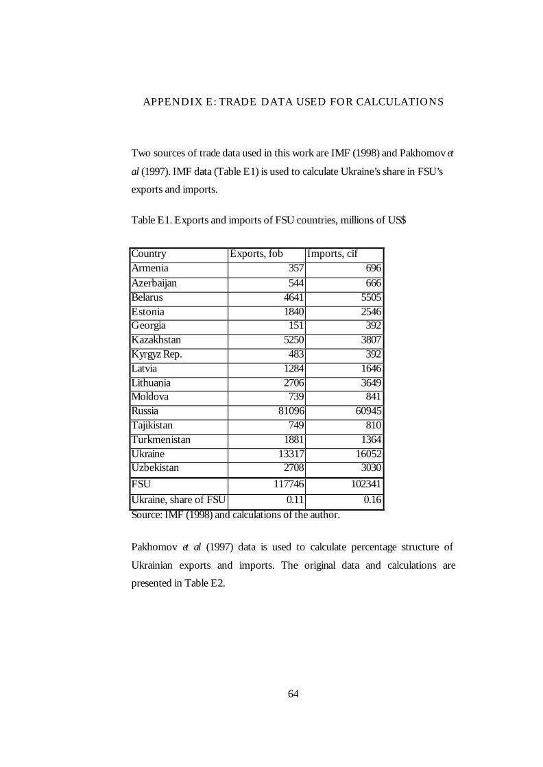
64

APPENDIX E: TRADE DATA USED FOR CALCULATIONS

Two sources of trade data used in this work are IMF (1998) and Pakhomov et

al (1997). IMF data (Table E1) is used to calculate Ukraine’s share in FSU’s

exports and imports.

Table E1. Exports and imports of FSU countries, millions of US$

Country Exports, fob Imports, cif Armenia 357 696 Azerbaijan 544 666 Belarus 4641 5505 Estonia 1840 2546 Georgia 151 392 Kazakhstan 5250 3807 Kyrgyz Rep. 483 392 Latvia 1284 1646 Lithuania 2706 3649 Moldova 739 841 Russia 81096 60945 Tajikistan 749 810 Turkmenistan 1881 1364 Ukraine 13317 16052 Uzbekistan 2708 3030

FSU 117746 102341

Ukraine, share of FSU 0.11 0.16 Source: IMF (1998) and calculations of the author.

Pakhomov et al (1997) data is used to calculate percentage structure of

Ukrainian exports and imports. The original data and calculations are

presented in Table E2.

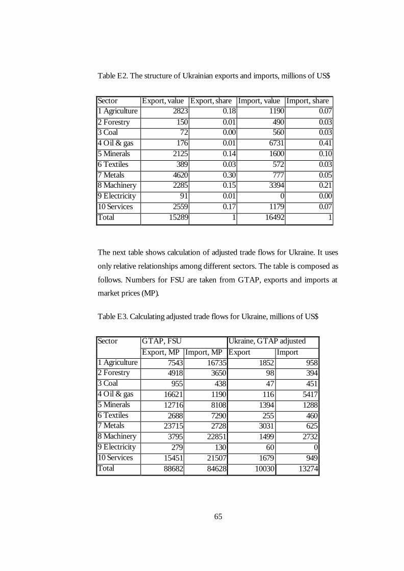
65

Table E2. The structure of Ukrainian exports and imports, millions of US$

Sector Export, value Export, share Import, value Import, share 1 Agriculture 2823 0.18 1190 0.07 2 Forestry 150 0.01 490 0.03 3 Coal 72 0.00 560 0.03 4 Oil & gas 176 0.01 6731 0.41 5 Minerals 2125 0.14 1600 0.10 6 Textiles 389 0.03 572 0.03 7 Metals 4620 0.30 777 0.05 8 Machinery 2285 0.15 3394 0.21 9 Electricity 91 0.01 0 0.00 10 Services 2559 0.17 1179 0.07 Total 15289 1 16492 1

The next table shows calculation of adjusted trade flows for Ukraine. It uses

only relative relationships among different sectors. The table is composed as

follows. Numbers for FSU are taken from GTAP, exports and imports at

market prices (MP).

Table E3. Calculating adjusted trade flows for Ukraine, millions of US$

GTAP, FSU Ukraine, GTAP adjusted Sector Export, MP Import, MP Export Import

1 Agriculture 7543 16735 1852 958 2 Forestry 4918 3650 98 394 3 Coal 955 438 47 451 4 Oil & gas 16621 1190 116 5417 5 Minerals 12716 8108 1394 1288 6 Textiles 2688 7290 255 460 7 Metals 23715 2728 3031 625 8 Machinery 3795 22851 1499 2732 9 Electricity 279 130 60 0 10 Services 15451 21507 1679 949 Total 88682 84628 10030 13274

66

Then the numbers for total adjusted export and import for Ukraine are

calculated using shares from Table E1, i.e. 10,030 = 0.11 * 88,682. Finally, the

value of each sector’s export and import is computed by applying weights

from Table E2 to just calculated total values. For example, adjusted export of

agriculture by Ukraine is computed by multiplying weight from Table E2 –

0.18 – by adjusted total exports – 10,030. The result – 1852 – is put down to

the forth column of Table E3.

Further, Ukrainian adjusted exports are divided by FSU exports from Table

E3 and the same is done for imports. Also, sum of Ukraine’s exports and

imports is divided by sum of FSU’s exports and imports to get weighting

coefficient for EV due to change in world prices. Computed weights are put

down into Table E4 and resemble Table 6 in the body of the thesis.

Table E4. Share of Ukraine’s trade in FSU’s trade

Sector Export and import Export Import 1 Agriculture 0.12 0.25 0.062 Forestry 0.06 0.02 0.113 Coal 0.35 0.05 1.004 Oil & gas 0.07 0.01 1.005 Minerals 0.13 0.11 0.166 Textiles 0.07 0.09 0.067 Metals 0.14 0.13 0.238 Machinery 0.16 0.39 0.129 Electricity 0.15 0.21 0.0010 Services 0.07 0.11 0.04

67

APPENDIX F: GDP DATA USED FOR CALCULATIONS

For disaggregating non-trade allocation effects is used the weighting

coefficient computed from table below. Input data are from the World Bank

(2001).

GDP at market prices (current $US millions), 1995 Armenia 2887 Azerbaijan 2894 Belarus 20071 Estonia 4789 Georgia 1900 Kazakhstan 19925 Kyrgyz Rep. 3325 Latvia 4904 Lithuania 6445 Moldova 3093 Russia 337902 Tajikistan 1827 Turkmenistan 4505 Ukraine 49061 Uzbekistan 16294

FSU 479822 Ukraine, share 0.1022 Source: World Bank (2001) and author’s calculations.