CUBE - User ManualGeneric Display for Application Performance Data

Version 2.0 / June 1, 2005

Fengguang Song, Felix Wolf

Copyright c© 2004 University of Tennessee

Contents

1 Introduction 3

2 Installation 4

2.1 Installing CUBE . . . . . . . . . . . . . . . . . . . . . . . . . . . . . . . . . .. . 4

2.2 Installing CUBE Library only . . . . . . . . . . . . . . . . . . . . . . .. . . . . 5

2.3 License . . . . . . . . . . . . . . . . . . . . . . . . . . . . . . . . . . . . . . . . 5

2.4 Libraries Required . . . . . . . . . . . . . . . . . . . . . . . . . . . . . . .. . . 5

2.5 Support . . . . . . . . . . . . . . . . . . . . . . . . . . . . . . . . . . . . . . . . 5

3 Using the Display 5

3.1 Basic Principles . . . . . . . . . . . . . . . . . . . . . . . . . . . . . . . . .. . . 6

3.2 GUI Components . . . . . . . . . . . . . . . . . . . . . . . . . . . . . . . . . . .7

3.2.1 Tree Browsers . . . . . . . . . . . . . . . . . . . . . . . . . . . . . . . . 7

3.2.2 Menu Bar . . . . . . . . . . . . . . . . . . . . . . . . . . . . . . . . . . . 8

3.2.3 Color Legend . . . . . . . . . . . . . . . . . . . . . . . . . . . . . . . . . 10

3.2.4 Status Bar . . . . . . . . . . . . . . . . . . . . . . . . . . . . . . . . . . . 10

3.2.5 Context Menus . . . . . . . . . . . . . . . . . . . . . . . . . . . . . . . . 10

3.3 Topology Display . . . . . . . . . . . . . . . . . . . . . . . . . . . . . . . . .. . 11

3.3.1 Menu Bar . . . . . . . . . . . . . . . . . . . . . . . . . . . . . . . . . . . 11

4 Performance Algebra 12

4.1 Difference . . . . . . . . . . . . . . . . . . . . . . . . . . . . . . . . . . . . . .. 12

4.2 Merge . . . . . . . . . . . . . . . . . . . . . . . . . . . . . . . . . . . . . . . . . 13

4.3 Mean . . . . . . . . . . . . . . . . . . . . . . . . . . . . . . . . . . . . . . . . . 13

4.4 Implementation . . . . . . . . . . . . . . . . . . . . . . . . . . . . . . . . . .. . 14

4.4.1 Integration of the Performance Space . . . . . . . . . . . . . .. . . . . . 14

4.4.2 Arithmetic Operation . . . . . . . . . . . . . . . . . . . . . . . . . . .. . 14

5 Tools 14

5.1 tau2cube . . . . . . . . . . . . . . . . . . . . . . . . . . . . . . . . . . . . . . . .14

6 Creating CUBE Files 15

6.1 CUBE API . . . . . . . . . . . . . . . . . . . . . . . . . . . . . . . . . . . . . . 15

6.1.1 Metric Dimension . . . . . . . . . . . . . . . . . . . . . . . . . . . . . . 15

6.1.2 Program Dimension . . . . . . . . . . . . . . . . . . . . . . . . . . . . . 16

6.1.3 System Dimension . . . . . . . . . . . . . . . . . . . . . . . . . . . . . . 17

6.1.4 Virtual Topologies . . . . . . . . . . . . . . . . . . . . . . . . . . . . .. 18

6.1.5 Severity Mapping . . . . . . . . . . . . . . . . . . . . . . . . . . . . . . .18

6.1.6 Miscellaneous . . . . . . . . . . . . . . . . . . . . . . . . . . . . . . . . 19

6.2 Typical Usage . . . . . . . . . . . . . . . . . . . . . . . . . . . . . . . . . . . .. 19

Abstract

CUBE is a generic presentation component suitable for displaying a wide variety of perfor-mance metrics for parallel programs includingMPI and OpenMP applications. Program per-formance is represented in a multi-dimensional space including various program and systemresources. The tool allows the interactive exploration of this space in a scalable fashion andbrowsing the different kinds of performance behavior with ease.CUBE also includes a libraryto read and write performance data as well as operators to compare, integrate, and summarizedata from different experiments. This user manual providesinstructions of how to installCUBE,how to use the display, how to use the operators, and how to write CUBE files.

1 Introduction

CUBE (CUBE Uniform Behavioral Encoding) is a generic presentation component suitable for dis-playing a wide variety of performance metrics for parallel programs includingMPI [2] and OpenMP

[3] applications.CUBE allows interactive exploration of a multidimensional metric space in a scal-able fashion. Scalability is achieved in two ways: hierarchical decomposition of individual dimen-sions and aggregation across different dimensions. All metrics are uniformly accommodated in thesame display and thus provide the ability to easily compare the effects of different kinds of programbehavior.

CUBE has been designed around a high-level data model of program behavior called theCUBE

performance space. TheCUBE performance space consists of three dimensions: a metric dimension,a program dimension, and a system dimension. The metric dimension contains a set of metrics, suchas communication time or cache misses. The program dimension contains the program’s call tree,which includes all the call paths onto which metric values can be mapped. The system dimensioncontains all the control flows of the program, which can be processes or threads depending onthe parallel programming model. Each point(m,c, l) of the space can be mapped onto a numberrepresenting the actual measurement for metricm while the control flowl was executing call pathc. This mapping is called theseverity of the performance space.

Each dimension of the performance space is organized in a hierarchy. First, the metric dimensionis organized in an inclusion hierarchy where a metric at a lower level is a subset of its parent, forexample, communication time is below execution time. Second, the program dimension is organizedin a call-tree hierarchy. Flat profiles can be represented asmultiple trivial call trees consisting onlyof a single node. Finally, the system dimension is organizedin a multi-level hierarchy consisting ofthe levels: machine,SMP node, process, and thread.

CUBE also includes a library to read and write instances of the previously described data model inthe form of anXML file. The file representation is divided into ametadata part and adata part. Themetadata part describes the structure of the three dimensions plus the definitions of various programand system resources. The data part contains the actual severity numbers to be mapped onto thedifferent elements of the performance space.

3

The display component can load such a file and display the different dimensions of the performancespace using three coupled tree browsers (Figure 1). The browsers are connected so that the usercan view one dimension with respect to another dimension. For example, the user can click on aparticular metric and see its distribution across the call tree. If theCUBE file contains topologicalinformation, the distribution of the performance metric across the topology can be examined usingtheCUBE topology view. Furthermore, the display is augmented with asource-code display that canshow the exact position of a call site in the source code.

As performance tuning of parallel applications usually involves multiple experiments to compare theeffects of certain optimization strategies,CUBE includes a new feature designed to simplify cross-experiment analysis. TheCUBE algebra [4] is an extension of the framework for multi-executionperformance tuning by Karavanic and Miller [1] and offers a set of operators that can be used tocompare, integrate, and summarize multipleCUBE data sets. The algebra allows the combination ofmultiple CUBE data sets into a single one that can be displayed like the original ones.

The following sections explain how to installCUBE, how to use the display, how to createCUBE

files, and how to use the algebra and other tools.

2 Installation

CUBE is available as a source-code distribution forUNIX platforms. You can downloadCUBE from:

http://icl.cs.utk.edu/kojak/cube/

Building CUBE requires theXML parser libxml2 and theGUI toolkit wxWidgets.

2.1 Installing CUBE

The full installation includes theCUBE library to createCUBE files, and theCUBE display componentto display their contents.

1. gunzip cube-2.0.tar.gz | tar xvf

2. cd cube-2.0

3. EditMakefile.defs

• Set the variablePREFIX to your desired installation path.

• Depending on the platform, select and uncomment a specific block corresponding toyour operating system. Available options areLINUX , AIX , IRIX , and SOLARIS. Tocustomize the compiler setting, please edit the following variables:

CCC: C++ compiler. Note that the compiler must be the same as the compiler used forcompilingWXWIDGETS, unless you build the library only.

CCFLAGS: C++ compiler options

LDFLAGS: Linker options

AR: Archive tool (e.g.,ar or CC)

ARFLAGS: Archive tool options

4

4. make

5. make install

2.2 Installing CUBE Library only

The partial installation will build and install only theCUBE library on your system. This is intendedfor users who just need to createCUBE file, but need not display it on their machines.

1. Same as steps of 1 to 3 described in the above section.

2. make lib

3. make install-lib

2.3 License

This software is free but by downloading and using it you automatically agree to comply with thelicense agreement. You can read the fileLICENSE in the distribution for precise wording.

2.4 Libraries Required

Both libraries listed below are necessary for using theCUBE display component. For those userswho need theCUBE library only, only libxml2 is required to be installed.

• libxml2 (2.5.6), which is an XML C parser and toolkit developed for the Gnome project. It ispre-installed on many systems. Please refer to the libxml2 web page for details:

http://xmlsoft.org/

• wxWidgets (2.4.2), which is a cross-platform C++ framework for writing advanced GUIapplications using native controls. Please refer to the wxWidgets web page for details:

http://www.wxwidgets.org/

2.5 Support

If you have any question or comments you would like to share with theCUBE developers, pleasesend e-mails tokojak@cs.utk.edu.

3 Using the Display

This section explains how to use theCUBE display component. After a brief description of the basicprinciples, different components of theGUI will be described in detail.

5

3.1 Basic Principles

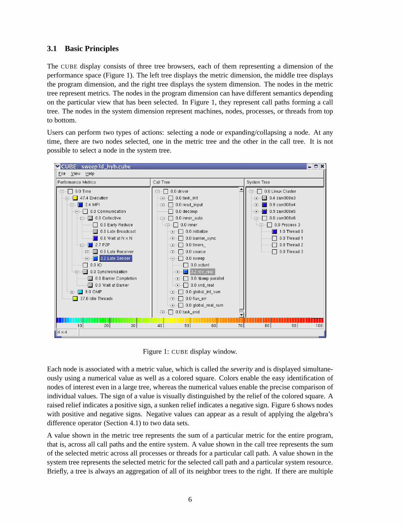
The CUBE display consists of three tree browsers, each of them representing a dimension of theperformance space (Figure 1). The left tree displays the metric dimension, the middle tree displaysthe program dimension, and the right tree displays the system dimension. The nodes in the metrictree represent metrics. The nodes in the program dimension can have different semantics dependingon the particular view that has been selected. In Figure 1, they represent call paths forming a calltree. The nodes in the system dimension represent machines,nodes, processes, or threads from topto bottom.

Users can perform two types of actions: selecting a node or expanding/collapsing a node. At anytime, there are two nodes selected, one in the metric tree andthe other in the call tree. It is notpossible to select a node in the system tree.

Figure 1:CUBE display window.

Each node is associated with a metric value, which is called theseverity and is displayed simultane-ously using a numerical value as well as a colored square. Colors enable the easy identification ofnodes of interest even in a large tree, whereas the numericalvalues enable the precise comparison ofindividual values. The sign of a value is visually distinguished by the relief of the colored square. Araised relief indicates a positive sign, a sunken relief indicates a negative sign. Figure 6 shows nodeswith positive and negative signs. Negative values can appear as a result of applying the algebra’sdifference operator (Section 4.1) to two data sets.

A value shown in the metric tree represents the sum of a particular metric for the entire program,that is, across all call paths and the entire system. A value shown in the call tree represents the sumof the selected metric across all processes or threads for a particular call path. A value shown in thesystem tree represents the selected metric for the selectedcall path and a particular system resource.Briefly, a tree is always an aggregation of all of its neighbortrees to the right. If there are multiple

6

call trees,CUBE has two options to compute the overall severity for a particular metric. Either itcan calculate the sum of all call trees (i.e., their root nodes in collapsed state) or their maximum. IfCUBE is unable to determine the correct mode it will ask the user.

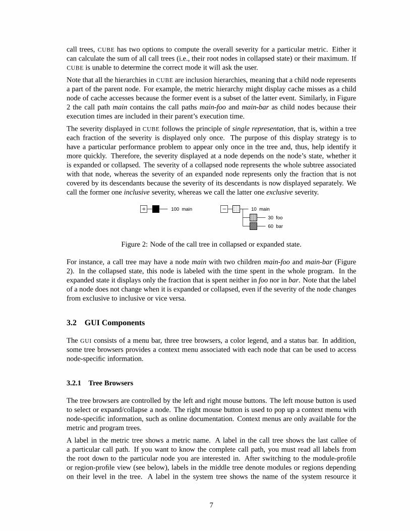
Note that all the hierarchies inCUBE are inclusion hierarchies, meaning that a child node representsa part of the parent node. For example, the metric hierarchy might display cache misses as a childnode of cache accesses because the former event is a subset ofthe latter event. Similarly, in Figure2 the call pathmain contains the call pathsmain-foo and main-bar as child nodes because theirexecution times are included in their parent’s execution time.

The severity displayed inCUBE follows the principle ofsingle representation, that is, within a treeeach fraction of the severity is displayed only once. The purpose of this display strategy is tohave a particular performance problem to appear only once inthe tree and, thus, help identify itmore quickly. Therefore, the severity displayed at a node depends on the node’s state, whether itis expanded or collapsed. The severity of a collapsed node represents the whole subtree associatedwith that node, whereas the severity of an expanded node represents only the fraction that is notcovered by its descendants because the severity of its descendants is now displayed separately. Wecall the former oneinclusive severity, whereas we call the latter oneexclusive severity.

10 main

30 foo

60 bar

100 main

Figure 2: Node of the call tree in collapsed or expanded state.

For instance, a call tree may have a nodemain with two childrenmain-foo andmain-bar (Figure2). In the collapsed state, this node is labeled with the timespent in the whole program. In theexpanded state it displays only the fraction that is spent neither in foo nor inbar. Note that the labelof a node does not change when it is expanded or collapsed, even if the severity of the node changesfrom exclusive to inclusive or vice versa.

3.2 GUI Components

The GUI consists of a menu bar, three tree browsers, a color legend, and a status bar. In addition,some tree browsers provides a context menu associated with each node that can be used to accessnode-specific information.

3.2.1 Tree Browsers

The tree browsers are controlled by the left and right mouse buttons. The left mouse button is usedto select or expand/collapse a node. The right mouse button is used to pop up a context menu withnode-specific information, such as online documentation. Context menus are only available for themetric and program trees.

A label in the metric tree shows a metric name. A label in the call tree shows the last callee ofa particular call path. If you want to know the complete call path, you must read all labels fromthe root down to the particular node you are interested in. After switching to the module-profileor region-profile view (see below), labels in the middle treedenote modules or regions dependingon their level in the tree. A label in the system tree shows thename of the system resource it

7

represents, such as a node name or a machine name. Processes and threads are usually identified bya number, but it is possible to give them specific names when creating aCUBE file. The thread levelof single-threaded applications is hidden. Note that all trees can have multiple root nodes.

Figure 3:CUBE menu bar.

3.2.2 Menu Bar

The menu bar consists of three menus, a file menu, a view menu, and a help menu.

FileThe file menu can be used to open and close a file and to exitCUBE.

ViewThe view menu (Figure 3) can be used to alter the way the program dimension is displayed, tochange the number representation for the entire display, orto hide positive or negative values.

After opening a data set the middle panel shows the call tree of the program - unless the dataset contains a flat profile. However, a user might wish to know which fraction of a metric canbe attributed to a particular region regardless of from where it was called. In this case, the usercan switch from the call-tree mode (default) to the module-profile mode or the region-profilemode (Figure 4). In the module-profile mode, the call-tree hierarchy is replaced with a source-code hierarchy consisting of three levels: module, region,and subregions. The subregions,if applicable, are displayed as a single child node labeledsubregions. A subregions noderepresents all regions directly called from the region above. In this way, the user is able to seewhich fraction of a metric is associated with a region exclusively, that is, without its regionscalled from there. The region-profile mode is similar to the module-profile mode except thatmodules are not shown.

The severity can be displayed in four different ways: as anabsolute value (default), aper-centage, arelative percentage, or as acomparative percentage. The absolute value is the realvalue measured. When displaying a value as a percentage, thepercentage refers to the value

8

shown at the root of the metric tree when it is in collapsed state. However, both absolute modeand percentage mode have the disadvantage that values can become very small the more yougo to the right, since aggregation occurs from right to left.To avoid this problem, the user canswitch to relative percentages. Then, a percentage in the right or middle tree always refers tothe selection in the neighbor to the left, that is, a percentage in the system dimension refersto the selection in the program dimension and a percentage inthe program dimension refersto the selected metric dimension. In this mode the percentages in the middle and right treealways sum up to one hundred percent. Figure 4 shows a region profile with relative percent-ages. Furthermore, to facilitate the comparison of different experiments, users can choose thecomparative percentage mode to display percentages relative to another data set. The com-parative percentage mode is basically like the normal percentage mode except that the valueequal to 100% is determined by another data set. Note that in the absolute mode, all valuesare displayed in scientific notation. To prevent clutteringthe display, only the mantissa isshown at the nodes with the exponent displayed at the color legend.

If one or more virtual topologies have been defined in theCUBE file, theTopology menu itemis enabled. Otherwise it is disabled. After selectingTopology, the Cartesian-selection dialogpops up if theCUBE file has multiple topologies. Through this dialog, users canchoose aspecific topology view to display in a topology window. Each topology is displayed in aseparate window. Please refer to Section 3.3 for detailed information.

Finally, to help users distinguish between positive and negative values more easily, users canhide either positive or negative values.

HelpCurrently, the help menu provides only an About dialog with release information.

Figure 4:CUBE module profile.

9

3.2.3 Color Legend

The color is taken from a spectrum ranging from blue to red representing the whole range of possiblevalues. To avoid an unnecessary distraction, insignificantvalues close to zero are displayed in darkgray. Exact zero values just have the background color. Depending on the severity representation,the color legend shows a numeric scale mapping colors onto values.

3.2.4 Status Bar

The first column showingm×n indicates that there arem processes and for each process there areat mostn threads in the execution.

3.2.5 Context Menus

The metric and program dimensions provide a context menu that can be used to obtain specificinformation on each node. The context menu is accessible viathe right mouse button. It displaysall or a subset of the options described below.

The call tree has a context menu consisting of two levels. Thefirst-level menu items areCall siteandCalled region. Choosing theCall site menu shows the information related to the call site, andchoosing theCalled region menu shows the information related to the region being called by thecall site (i.e., the callee).

Location: Displays the source-code location of a program resource in textual form (i.e., at whichline and in what module). In the module-profile and region-profile modes, it always refersto the location of its associated region. In the call-tree mode, a call-tree node is usuallyassociated with two entities: a callsite and the region called by the callsite. By entering aspecific level of the context menu:Callsite or Called region, users are able to check either theassociated call site’s or the called region’s location. Forthe call site, it shows the call site’slocation where it has been called or its calling region’s location if the line number of the callsite is undefined. For the called region, it shows the location of the region being called by thecall site.

Source code: Displays and highlights the source code of a program resource in the source codebrowser. In the module-profile and region-profile modes, it always shows and highlights thesource code of its associated region. In the call-tree mode,since each call-tree node has acontext menu of two levels, by choosing theCall site menu it displays and highlights thesource code of the call site or the block of source code of the calling region. And by choosingtheCalled region menu it displays and highlights the block of code of the region being calledby the call site. Note that not all data sets provide sufficient line-number information to showthe correct section of the source code.

Online description: Both metrics and regions can be linked to an online description. For ex-ample, metrics might point to an online documentation explaining their semantics, or regionsrepresenting library functions might point to the corresponding library documentation.

Info: A brief description of metrics or regions supplied by theCUBE data set.

10

3.3 Topology Display

In many parallel applications, each process (or thread) communicates only with a limited number ofprocesses. The parallel algorithm divides the applicationdomain into smaller chunks known as subdomains. A process usually communicates with processes owning sub domains adjacent to its own.The mapping of data onto processes and the neighborhood relationship resulting from this mappingis calledvirtual topology. Many applications use one or more virtual topologies (Figure 5) specifiedas one-, two- or three- dimensional Cartesian grids. TheCUBE topology display shows performancedata mapped onto the Cartesian topology of the application.The corresponding grid is specified bytwo parameters: number of dimensions and size of each dimension

Figure 5: Topology display

The display consists of a menu bar andthe actual Cartesian grid. The Cartesiangrid is presented by planes stacked on topof each other in a three dimensional pro-jection. The number of planes dependson the number of dimensions in the grid.Each plane is divided into squares. Thenumber of squares depends on the dimen-sion size. Each square represents a systemresource (e.g a process) of the applicationand has a coordinate associate with it.

The grid displays the severity of the se-lected metric in the selected call path foreach system resource participating in theapplication’s topology. The severity isrepresented as a color. A system resourcemight not be a part of the application’svirtual topology or may have a zero value for a metric. Therefore, it is sometimes possible tohave some uncolored squares in the grid picture.

3.3.1 Menu Bar

The menu bar consists of four menus: a view menu, a geometry menu, a zoom menu and, a colorsmenu.

View: The view menu can be used to choose one of the three possible orientations of the grid. Thecoordinate axes at the bottom of the picture indicate the direction of X, Y and Z dimensionsin the three-dimensional space. In case of one- or two- dimensional grids, users are providedwith only one orientation of the grid.

Geometry: Due to varying dimension sizes, planes in the grid might overlap with each other andthe size of the squares might be too small to recognize their color. This may pose a problemfor the user to view the topology information effectively. The geometry menu circumventsthis problem by providing options to scale the picture in various ways. TheAngle option helpsthe user to adjust the skew of the three-dimensional projection. ThePlane Distance optionhelps to adjust the inter-plane distance. ThePlane Length option helps users scale the area ofeach plane.

11

Zoom: The zoom menu can be used to zoom-in or zoom-out on the grid.

Colors: The colors menu can be used to modify the text color and the background color of thetopology display. Finally, there are two resolution modes to choose from. TheLow Resolutionmode assigns colors to the squares according to the severityvalues shown in the systemdimension. Often, these values have small variations from each other and do not help the userto study the relative distribution of severities across thegrid. To exploit the entire spectrum ofavailable colors and to enable the user to study the relativedistribution of severities, aHighResolution mode is provided. This mode highlights the minute differences between severityvalues of the system resources. Severity values of zero are assigned the background color ofthe display. This mode has its own color legend showing the minimum and maximum valuesfor the selected severities across the grid. These values can be absolute values, percentages,or relative percentages depending on theCUBE view mode.

4 Performance Algebra

As performance tuning of parallel applications usually involves multiple experiments to comparethe effects of certain optimization strategies,CUBE offers a mechanism calledperformance algebrathat can be used to merge, subtract, and average the data fromdifferent experiments and and viewthe results in the form of a single “derived” experiment. Using the same representation for derivedexperiments and original experiments provides access to the derived behavior based on familiarmetaphors and tools in addition to an arbitrary and easy composition of operations. The algebra isan ideal tool to verify and locate performance improvementsand degradations likewise. The algebraincludes three operatorsdiff, merge, andmean provided as command-line utilities which take two ormoreCUBE files as input and generate anotherCUBE file as output. The operations are closed in thesense that the operators can be applied to the results of previous operations. Note that although alloperators are defined for any validCUBE data sets, not all possible operations make actually sense.For example, whereas it can be very helpful to compare two versions of the same code, computingthe difference between entirely different programs is unlikely to yield any useful results.

4.1 Difference

Changing a program can alter its performance behavior. Altering the performance behavior meansthat different results are achieved for different metrics.Some might increase while others mightdecrease. Some might rise in certain parts of the program only, while they drop off in other parts.Finding the reason for a gain or loss in overall performance often requires considering the perfor-mance change as a multidimensional structure. WithCUBE’s difference operator, a user can viewthis structure by computing the difference between two experiments and rendering the derived re-sult experiment like an original one. The difference operator takes two experiments and computes aderived experiment whose severity function reflects the difference between the minuend’s severityand the subtrahend’s severity.

Figure 6 shows the difference betweenKOJAK [5] analysis results obtained from the original and anoptimized version of a nano-particle simulation. Raised reliefs indicate performance improvements,and sunken reliefs indicate performance degradations. Thefigure indicates that a certain optimiza-tion was only partially successful because some of the wait states migrated to other locations in theprogram instead of disappearing.

12

Usage: cube diff <minuend> <subtrahend> [-o <output>]

The default output file name isdiff.cube.

Figure 6: A derived experiment computed usingcube diff.

4.2 Merge

The merge operator’s purpose is the integration of performance data from different sources. Often acertain combination of performance metrics cannot be measured during a single run. For example,certain combinations of hardware events cannot be counted simultaneously due to hardware resourcelimits. Or the combination of performance metrics requiresusing different monitoring tools thatcannot be deployed during the same run. The merge operator takes twoCUBE experiments witha different or overlapping set of metrics and yields a derived CUBE experiment with a joint set ofmetrics.

Usage: cube merge <op1> <op2> [-o <output>]

The default output file name ismerge.cube.

4.3 Mean

The mean operator is intended to smooth the effects of randomerrors introduced by unrelated systemactivity during an experiment or to summarize across a rangeof execution parameters. The user canconduct several experiments and create a single average experiment from the whole series. Differentfrom the previous tow operators, which are binary operators, the mean operator takes an arbitrarynumber of arguments.

Usage: cube mean <op1> <op2> ...<opN> [-o <output>]

The default output file name ismerge.cube.

13

4.4 Implementation

The actions performed by the operators can be divided into two subtasks: integration of the perfor-mance space followed by the actual arithmetic operation.

4.4.1 Integration of the Performance Space

The integration of two or more performance spaces consists of three separate parts: merging themetric dimension, merging the program dimension, and merging the system dimension. Mergingmetric trees and call trees works very similar to the structural merge operator in [1]. While traversingfrom the roots to the leaves,CUBE tries to match up the nodes. Nodes that cannot be matched areseparately included in the new performance space, whereas nodes that can be successfully matchedbecome shared nodes, that is, they appear as a single node in the new space.

Merging the system dimension is slightly different. There are four levels with different mean-ings: machine, node, process, and thread. First, processesand threads are matched based on theirapplication-level identifiers, for example, their globalMPI rank andOpenMP thread number. Next,CUBE examines whether the partitioning of processes into nodes is compatible between the twooperands. If compatible,CUBE copies the entire node and machine hierarchy including the corre-sponding process-node mapping of one of the operands into the result. Otherwise it collapses themachine and node level into a single machine and a single node.

4.4.2 Arithmetic Operation

After performance-space integration, a new severity function is computed whose domain is theintegrated space. An element-wise operation is performed on the two input arrays. To be ableto perform an element-wise operation, the operand’s severity function is extended with respect tothe integrated metadata so that it is defined for every tuple (metric, call path, thread) of the newmetadata. This is done by assigning zero to previously undefined tuples. For example, a call pathoccurring in one metadata set might not occur in another. If this happens the resulting value for thiscall path will be set to zero in those experiments that didn’tcontain the call path before.

In the case of the difference or the mean operators, the element-wise operation is just a subtractionor arithmetic mean operation, respectively. In the case of the merge operatorCUBE makes a simplecase distinction. Recall that the purpose of doing the mergeoperation is to integrate performance ex-periments with different metrics. For example, one experiment counts floating point operations, andthe other one counts cache misses, since we might not be able to count both of them simultaneously.So, if the metric is provided only by one experimentCUBE takes the data from that experiment. If itis provided by both experimentsCUBE takes it from the first one (without loss of generality).

5 Tools

5.1 tau2cube

TAU is designed to provide a framework for integrating program and performance analysis tools andcomponents. Using the tool oftau2cube, TAU profiles are able to be converted to theCUBE format.

14

Usage: tau2cube [<tau-profile-dir>] [-o <output>]

The first parameter is theTAU profile directory. The second parameter is the name of theoutput CUBE file. The default for<tau-profile-dir> is the current directory and the defaultoutput file name isa.cube.

Limitations:

• Converts only flat, two-level (one level more than flat), or full call path profiles (all callers upto main).

• The main function must be included and every other function must be called from withinmain. Static initializers outside the main function are notsupported.

6 Creating CUBE Files

The CUBE data format in anXML instance [6]. The correspondingXMLSchema specification [7]can be found indoc/cube.xsd in theCUBE distribution. TheCUBE library provides an interface tocreateCUBE files. It is a simple class interface and includes only a few methods. This section firstdescribes theCUBE API and then presents a simple C++ program as an example of how to use it.

6.1 CUBE API

The class interface defines aclass Cube. The class provides a default constructor and sixteenmethods. The methods are divided into four groups. The first three groups are used to define thethree dimensions of the performance space and the last groupis used to enter the actual data. Inaddition, an output operator<< to write the data to a file is provided.

The methods used to create the different entities of the performance space always return aconstobject pointer which can be used for further reference.

6.1.1 Metric Dimension

This group refers to the metric dimension of the performancespace. It consist of a single methodused to build metric trees. Each node in the metric tree represents a performance metric. Met-rics have different units of measurement. The unit can be either “sec” (i.e., seconds) for timebased metrics, such as execution time, or “occ” (i.e., occurrences) for event-based metrics, such asfloating-point operations. During the establishment of a metric tree, a child metric is usually morespecific than its parent, and both of them have same unit of measurement. Thus, a child performancemetric has to be a subset of its parent metric (e.g., system time is a subset of execution time).

const Metric* def met (string name, string uom, string url,string descr, const Metric* parent);

Returns a metric with namename and descriptiondescr. uom specifies the unit of measure-ment, which is either “sec” for seconds or “occ” for number of occurrences.parent is apreviously created metric which will be the new metric’s parent. To define a root node, useNULL instead.url is a link to anHTML page describing the new metric in detail. If you want

15

to mirror the page at several locations, you can use the macro@mirror@ as a prefix, whichwill be replaced by an available mirror defined usingdef mirror() (see Section 6.1.6).

6.1.2 Program Dimension

This group refers to the program dimension of the performance space. The entities presented in thisdimension aremodule, region, call site, andcall-tree node (i.e., call paths). A module is a sourcefile, which can contain several code regions. A region can be afunction, a loop, or a basic block.Each region can have multiple call sites from which the control flow of the program enters a newregion. Although we use the term call site here, any place that causes the program to enter a newregion can be represented as a call site, including loop entries. Correspondingly, the region enteredfrom a call site is calledcallee, which might as well be a loop. Every call-tree node points toa callsite. The actual call path represented by a call-tree node can be derived by following all the call sitesstarting at the root node and ending at the particular node ofinterest. Therefore, before defining acall-tree node, the necessary call sites, callees, and modules have to be defined. The user can choseamong three ways of defining the program dimension:

1. Call tree with line numbers

2. Call tree without line numbers

3. Flat profile

A call tree with line numbers is defined as a tree whose nodes point to call sites. A call tree withoutline numbers is defined as a tree whose nodes point to regions (i.e., the callees). A flat profile issimply defined as a set of regions, that is, no tree has to be defined.

const Module* def module (string name);

Returns a new module with module namename, which can be either a complete path or a filename.

const Region* def region (string name, long begln, long endln,string url, string descr,const Module* mod);

Returns a new region with region namename and descriptiondescr. The region is locatedin the modulemod and exists from linebegln to line endln. url is a link to anHTML pagedescribing the new metric in detail. If you want to mirror thepage at several locations, youcan use the macro @mirror@ as a prefix, which will be replaced by an available mirrordefined usingdef mirror() (see Section 6.1.6).

const Callsite* def csite (const Module* mod, int line,const Region* callee);

Returns a new a call site located at the lineline of the modulemod. The call site calls thecalleecallee (i.e., a previously defined region).

const Cnode* def cnode (const Callsite* csite,const Cnode* parent);

16

Returns a new call-tree node representing a call from call site csite. parent is a previouslycreated call-tree node which will be the new one’s parent. Todefine a root node, useNULLinstead. This method is used to create a call tree with line numbers.

const Cnode* def cnode (const Region* region,const Cnode* parent);

Defines a new call-tree node representing a call to the regionregion. parent is a previouslycreated call-tree node which will be the new one’s parent. Todefine a root node, useNULLinstead. Note that different from the previousdef cnode(), this method is used to create acall-tree without line numbers where each call-tree node points to a region, instead of a callsite.

To define a call tree with line numbers usedef csite() anddef cnode(const Callsite*...).To define a call tree without line numbers usedef cnode(const Region*...). To create a flatprofile use neither one - just defining a set of regions will be sufficient.

6.1.3 System Dimension

This group refers to the system dimension of the performancespace. It reflects the system resourceson which the program is using at runtime. The entities present in this dimension aremachine, node,process, and thread, which populate four levels of the system hierarchy in the given order. Thatis, the first level consists of machines, the second level of nodes, and so on. Finally, the last (i.e.,leaf) level is populated only by threads. The system tree is built in a top-down way starting with amachine. Note that even if every process has only one thread,users still need to define the threadlevel.

const Machine* def mach (string name);

Returns a new machine with the namename.

const Node* def node (string name, const Machine* mach);

Returns a new (SMP) node which has the namename and which belongs to the machinemach.

const Process* def proc (string name, int rank,const Node* node);

Returns a new process which has the namename and the rankrank. The rank is a numberfrom 0− (n−1), wheren is the total number of processes.MPI applications may use the rankin MPI COMM WORLD. The process runs on the nodenode.

const Thread* def thrd (string name, int rank,const Process* proc);

Defines a new thread which has the namename and the rankrank. The rank is a numberfrom 0− (n − 1), wheren is the total number of threads spawned by a process. OpenMP

applications may use the OpenMP thread number. The thread belongs to the processproc.

17

6.1.4 Virtual Topologies

Virtual topologies are used to describe adjacency relationships among machines,SMP nodes, pro-cesses or threads. A topology usually consists of a single class of entities such as threads or pro-cesses. TheCUBE API provides a set of functions to create Cartesian topologies and to define themachine/SMP node/process/thread mappings onto coordinates. Note thatthe definition of virtualtopologies is optional.

const Cartesian* def cart (long ndims, const vector<long>& dimv,const vector<bool>& periodv);

Defines a new Cartesian topology.ndims anddimv specify the number of dimensions and thesize of each dimension.periodv specifies the periodicity for each dimension.

void def coords (const Cartesian* cart, const Location* loc,const vector<long>& coordv);

Maps a specific location onto a Cartesian coordinate. The location loc may be a machine,SMP node, process or a thread. It is not recommended to map a mixedset of entities ontoone topology (e.g., machines and threads are located in the same topology). The parameterof cart has been defined by the abovedef cart() method.

6.1.5 Severity Mapping

After the establishment of performance space, users can assign severity values to points of thespace. Each point is identified by a tuple(met, cnode, thrd). The value should be inclusivewith respect to the metric, but exclusive with respect to thecall-tree node, that is it should not coverits children. Taking Figure 2 as an example, this means that if the value refers tomain then it shouldnot includemain-foo or main-bar. The default severity value for the data points left undefined iszero. Thus, users only need to define non-zero data points.

void set sev (const Metric* met, const Cnode* cnode,const Thread* thrd, double value);

Assigns the valuevalue to the point(met, cnode, thrd).

void add sev (const Metric* met, const Cnode* cnode,const Thread* thrd, double value);

Adds the valuevalue to the present value at point(met, cnode, thrd).

The previous two methodsset sev() andadd sev() are intended to be used when the programdimension contains a call tree and not a flat profile. As the flatprofile does not require the definitionof call-tree nodes, the following two functions should be used instead:

void set sev (const Metric* met, const Region* region,const Thread* thrd, double value);

Assigns the valuevalue to the point(met, region, thrd).

void add sev (const Metric* met, const Region* region,const Thread* thrd, double value);

Adds the valuevalue to the present value at point(met, region, thrd).

18

6.1.6 Miscellaneous

Often users may want to define some information related to theCUBE file itself, such as the creationdate, experiment platform, and so on. For this purpose,CUBE allows the definition of arbitraryattributes in everyCUBE data set. An attribute is simply a key-value pair and can be defined usingthe following method:

void def attr (string key, string value);

Assigns the valuevalue to the attributekey.

There is one predefined attributeCUBE CT AGGR with valuesMAX andSUM to stipulate the aggre-gation mode applied in the presence of multiple call trees (Section 3.1). If this attribute is definedCUBE will use the specified mode and suppress the input dialog.

CUBE allows using multiple mirrors for the online documentationassociated with metrics and re-gions. Theurl expression supplied as an argument fordef metric() and def region() cancontain a prefix@mirror@. When the online documentation is accessed,CUBE can substitute allmirrors defined for the prefix until a valid one has been found.If no valid online mirror can befound,CUBE will substitute the./doc directory of the installation path for@mirror@.

void def mirror (string mirror);

Defines the mirrormirror as potential substitution for theURL prefix@mirror@.

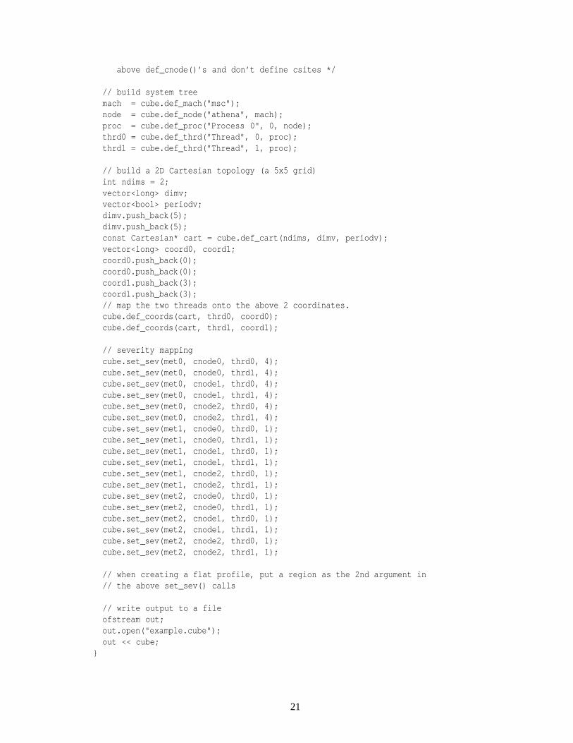
6.2 Typical Usage

A simple C++ program is given to demonstrate how to use theCUBE write interface. Figure 7 showsthe correspondingCUBE display. The source code of the target application is provided in Figure 8.

Figure 7: Display ofexample.cube

// A C++ example using CUBE write interfaceint main(int argc, char* argv[]) {// Declarations (All const class pointers)

...

Cube cube;

// specify mirrors (optional)

19

1 void foo() {...

10 }11 void bar() {

...20 }21 int main(int argc, char* argv) {

...60 foo();

...80 bar();

...100 }

Figure 8: Target-application source codeexample.c

cube.def_mirror("http://icl.cs.utk.edu/software/kojak/");cube.def_mirror("http://www.fz-juelich.de/zam/kojak/");

// specify information related to the file (optional)cube.def_attr("experiment time", "November 1st, 2004");cube.def_attr("description", "a simple example");

// build metric treemet0 = cube.def_met("Time", "sec",

"@mirror@patterns-2.1.html#execution","root node", NULL); // using mirror

met1 = cube.def_met("User time", "sec","http://www.cs.utk.edu/usr.html","2nd level", met0); // withoug using mirror

met2 = cube.def_met("System time", "sec","http://www.cs.utk.edu/sys.html","2nd level", met0); // withoug using mirror

// build a call tree with line numbersmod = cube.def_module("/ICL/CUBE/example.c");regn0 = cube.def_region("main", 21, 100, "", "1st level", mod);regn1 = cube.def_region("foo", 1, 10, "", "2nd level", mod);regn2 = cube.def_region("bar", 11, 20, "", "2nd level", mod);

// When creating flat profiles, you do not need// define call sites and call-tree nodes.csite0 = cube.def_csite(mod, 21, regn0);csite1 = cube.def_csite(mod, 60, regn1);csite2 = cube.def_csite(mod, 80, regn2);cnode0 = cube.def_cnode(csite0, NULL);cnode1 = cube.def_cnode(csite1, cnode0);cnode2 = cube.def_cnode(csite2, cnode0);/* If creating call trees without line numbers,

put a region as the 1st argument in the

20

above def_cnode()’s and don’t define csites */

// build system treemach = cube.def_mach("msc");node = cube.def_node("athena", mach);proc = cube.def_proc("Process 0", 0, node);thrd0 = cube.def_thrd("Thread", 0, proc);thrd1 = cube.def_thrd("Thread", 1, proc);

// build a 2D Cartesian topology (a 5x5 grid)int ndims = 2;vector<long> dimv;vector<bool> periodv;dimv.push_back(5);dimv.push_back(5);const Cartesian* cart = cube.def_cart(ndims, dimv, periodv);vector<long> coord0, coord1;coord0.push_back(0);coord0.push_back(0);coord1.push_back(3);coord1.push_back(3);// map the two threads onto the above 2 coordinates.cube.def_coords(cart, thrd0, coord0);cube.def_coords(cart, thrd1, coord1);

// severity mappingcube.set_sev(met0, cnode0, thrd0, 4);cube.set_sev(met0, cnode0, thrd1, 4);cube.set_sev(met0, cnode1, thrd0, 4);cube.set_sev(met0, cnode1, thrd1, 4);cube.set_sev(met0, cnode2, thrd0, 4);cube.set_sev(met0, cnode2, thrd1, 4);cube.set_sev(met1, cnode0, thrd0, 1);cube.set_sev(met1, cnode0, thrd1, 1);cube.set_sev(met1, cnode1, thrd0, 1);cube.set_sev(met1, cnode1, thrd1, 1);cube.set_sev(met1, cnode2, thrd0, 1);cube.set_sev(met1, cnode2, thrd1, 1);cube.set_sev(met2, cnode0, thrd0, 1);cube.set_sev(met2, cnode0, thrd1, 1);cube.set_sev(met2, cnode1, thrd0, 1);cube.set_sev(met2, cnode1, thrd1, 1);cube.set_sev(met2, cnode2, thrd0, 1);cube.set_sev(met2, cnode2, thrd1, 1);

// when creating a flat profile, put a region as the 2nd argument in// the above set_sev() calls

// write output to a fileofstream out;out.open("example.cube");out << cube;

}

21

References

[1] K. L. Karavanic and B. Miller. A Framework for Multi-Execution Performance Tuning.Paralleland Distributed Computing Practices, 4(3), September 2001. Special Issue on MonitoringSystems and Tool Interoperability.

[2] Message Passing Interface Forum.MPI: A Message Passing Interface Standard, June 1995.http://www.mpi-forum.org.

[3] OpenMP Architecture Review Board.OpenMP Fortran Application Program Interface - Ver-sion 2.0, November 2000.http://www.openmp.org.

[4] F. Song, F. Wolf, N. Bhatia, J. Dongarra, and S. Moore. An Algebra for Cross-ExperimentPerformance Analysis. InProc. of ICPP 2004, pages 63–72, Montreal, Canada, August 2004.

[5] F. Wolf and B. Mohr. Automatic performance analysis of hybrid MPI/OpenMP applications.Journal of Systems Architecture, 49(10-11):421–439, 2003. Special Issue “Evolutions in paral-lel distributed and network-based processing”.

[6] World Wide Web Consortium.Extensible Markup Language (XML) 1.0 (Second Edition), Oc-tober 2000.http://www.w3.org/TR/REC-xml.

[7] World Wide Web Consortium.XML Schema Part 0, 1, 2, May 2001. http://www.w3.org/XML/Schema#dev.

22