CSAE Working Paper WPS/2014-37 · third-party randomly split our dataset in two and gave us sample...
80
Centre for the Study of African Economies Department of Economics . University of Oxford . Manor Road Building . Oxford OX1 3UQ T: +44 (0)1865 271084 . F: +44 (0)1865 281447 . E: [email protected] . W: www.csae.ox.ac.uk Do Politicians’ Relatives Get Better Jobs? Evidence from Municipal Elections Marcel Fafchamps and Julien Labonne ∗ December 2014 Abstract We estimate the impacts of being connected to politicians on occupational choice. We use an administrative dataset collected in 2008-2010 on 20 million individuals and rely on naming conventions to assess family links to candidates in elections held in 2007 and 2010. We first estimate the value of political connections by applying a regression discontinuity design to close elections in 2007. Those estimates likely combine the benefits from connections to current office-holders and the cost associated with being related to a losing candidate. We use individuals connected to successful candidates in the 2010 elections as control group and find that relatives of current office-holders are more likely to employed in better paying occupations. Relatives of candidates who narrowly lost in 2007 have lower occupations. A third-party randomly split our dataset in two and gave us sample 1. Once the review is completed, we will apply the approved methodology to sample 2. ∗ Fafchamps: Stanford University, Freeman Spogli Institute for International Studies, Encina Hall E105, Stan- ford CA 94305 USA ([email protected]). Labonne: Oxford University, Blavatnik School of Government, 10 Merton Street, Oxford OX1 4JJ, United Kingdom ([email protected]). An earlier version of this paper was circulated under the title ‘Nepotism and Punishment: the (Mis-)Performance of Elected Local Officials in the Philippines’. We are indebted to Lorenzo Ductor for agreeing to act as the third party who performed the random sample split. The Department of Social Welfare and Development kindly allowed us to use data from the National Household Targeting System for Poverty Reduction and Pablo Querubin kindly shared some electoral data. We thank Fermin Adriano, Farzana Afridi, Sam Asher, Jean-Marie Baland, Hrithik Bansal, Andrew Beath, Cesi Cruz, Lorenzo Ductor, Taryn Dinkelman, Motoky Hayakawa, Bert Hofman, Clement Imbert, Philip Keefer, Claire Labonne, Horacio Larreguy, Clare Leaver, Pablo Querubin, Simon Quinn, Ronald Rogowski, Matt Stephens and Kate Vyborny as well as seminar and conference participants in the CSAE 2012, South East Asia Sympo- sium 2012, Gorman Workshop, UPSE, AIM Policy Center, DIAL 2013, CMPO Political Economy and Public Services workshop 2013, IFS/EDEPO, RECODE, CERDI, NEUDC 2013, Blavatnik School of Government, NYU Abu Dhabi, IIES, Monash, Yale-NUS, CGD, World Bank and Ateneo School of Government for comments. All remaining errors are ours. 1 CSAE Working Paper WPS/2014-37
Transcript of CSAE Working Paper WPS/2014-37 · third-party randomly split our dataset in two and gave us sample...

Centre for the Study of African EconomiesDepartment of Economics . University of Oxford . Manor Road Building . Oxford OX1 3UQT: +44 (0)1865 271084 . F: +44 (0)1865 281447 . E: [email protected] . W: www.csae.ox.ac.uk
Do Politicians’ Relatives Get Better Jobs?
Evidence from Municipal Elections
Marcel Fafchamps and Julien Labonne∗
December 2014
Abstract
We estimate the impacts of being connected to politicians on occupational choice. We usean administrative dataset collected in 2008-2010 on 20 million individuals and rely on namingconventions to assess family links to candidates in elections held in 2007 and 2010. We firstestimate the value of political connections by applying a regression discontinuity design toclose elections in 2007. Those estimates likely combine the benefits from connections tocurrent office-holders and the cost associated with being related to a losing candidate. Weuse individuals connected to successful candidates in the 2010 elections as control groupand find that relatives of current office-holders are more likely to employed in better payingoccupations. Relatives of candidates who narrowly lost in 2007 have lower occupations. Athird-party randomly split our dataset in two and gave us sample 1. Once the review iscompleted, we will apply the approved methodology to sample 2.
∗Fafchamps: Stanford University, Freeman Spogli Institute for International Studies, Encina Hall E105, Stan-ford CA 94305 USA ([email protected]). Labonne: Oxford University, Blavatnik School of Government, 10Merton Street, Oxford OX1 4JJ, United Kingdom ([email protected]). An earlier version of this paperwas circulated under the title ‘Nepotism and Punishment: the (Mis-)Performance of Elected Local Officials inthe Philippines’. We are indebted to Lorenzo Ductor for agreeing to act as the third party who performed therandom sample split. The Department of Social Welfare and Development kindly allowed us to use data from theNational Household Targeting System for Poverty Reduction and Pablo Querubin kindly shared some electoraldata. We thank Fermin Adriano, Farzana Afridi, Sam Asher, Jean-Marie Baland, Hrithik Bansal, Andrew Beath,Cesi Cruz, Lorenzo Ductor, Taryn Dinkelman, Motoky Hayakawa, Bert Hofman, Clement Imbert, Philip Keefer,Claire Labonne, Horacio Larreguy, Clare Leaver, Pablo Querubin, Simon Quinn, Ronald Rogowski, Matt Stephensand Kate Vyborny as well as seminar and conference participants in the CSAE 2012, South East Asia Sympo-sium 2012, Gorman Workshop, UPSE, AIM Policy Center, DIAL 2013, CMPO Political Economy and PublicServices workshop 2013, IFS/EDEPO, RECODE, CERDI, NEUDC 2013, Blavatnik School of Government, NYUAbu Dhabi, IIES, Monash, Yale-NUS, CGD, World Bank and Ateneo School of Government for comments. Allremaining errors are ours.
1
CSAE Working Paper WPS/2014-37

1 Introduction
In this paper we examine whether people who are related to a successful politician get a better
job. This could arise for different reasons. One possibility is nepotism – politicians could
favor their relatives in public sector jobs, either because of redistributive norms/altruism, or
as a reward for their political support. Another possibility is loyalty or screening – politicians
may search among their relatives the able and reliable workers they need to implement their
policies (Iyer and Mani 2012). It is also conceivable that employers recruit the elected officials’
relatives in the hope of securing political support and protection. We test whether a successful
politician’s relatives are more likely to be employed in a higher-ranked, better paid occupation
in the public or private sector. Evidence in support of this hypothesis would have implications
for political economy models emphasizing the principal-agent relationships between politicians
and either bureaucrats or firms. For example, if politicians are able to staff the bureaucracy
with their relatives then the principal-agent problem in the relationship between politicians and
bureaucrats might be overstated.
The literature on the value of political connections for individuals has faced several difficulties
and is not well-developed.1 First, for lack of better data, researchers often rely on self-reported
links to local politicians as a measure of political connections. Such data are subject to bias
because the likelihood of reporting connections might be correlated with the benefits that are
derived from them (Comola and Fafchamps forthcoming). Second, individuals connected to
politicians may differ from the average citizen along unobservable characteristics that affect
1Thanks to panel data, progress has been made on establishing the value of political connections for firms(Fisman 2001, Khwaja and Mian 2005, Faccio 2006, Cingano and Pinotti 2013). Studies have established thatpolitical connections, either fixed ties (such as family ties) or more direct investment (such as campaign contri-butions) are valuable in the sense the connected firms tend to have higher stock market valuations. This is afeature of both developed and developing economies and those effects tend to be higher in countries with higherlevels of corruption (Faccio 2006). A number of channels have been identified, the most common of which beingthat connected firms are more likely to benefit from procurement contracts, tend to enjoy lower cost of capitaland more favorable regulatory environment. A related literature has explored the private returns to holding officeand has found that politicians’ assets tend to grow faster either while in office or once they’ve left (Eggers andHainmueller 2009, Fisman, Schulz and Vig forthcoming, Querubin and Snyder 2013). Less progress has beenmade in identifying the value of political connections for individuals (Besley, Pande and Rao 2012, Blanes i Vi-dal, Draca and Fons-Rosen 2012, Caeyers and Dercon 2012, Markussen and Tarp forthcoming, Gagliarducci andManacorda 2014). This is related to the literature on the role of family links in labor markets. For example,Wang (2013) documents a significant reduction in earnings when a man’s father-in-law dies.
2
their welfare even when their politician relatives are not in office (Besley 2005). It follows that
when researchers observe a correlation between individual welfare and political connections, it is
unclear how much of this correlation is due to unobserved heterogeneity. Third, the literature on
the value of political connections has not accounted for the possibility that individuals connected
to politicians who lost an election can suffer from their connections, especially in areas where
elected officials have discretionary powers.
Using a large dataset from the Philippines, collected between the 2007 and 2010 municipal
elections, we test whether individuals who are connected to politicians in municipal elections are
employed in better-paying occupations.2 We contribute to the literature on the value of political
connections in three ways. First, we distinguish between individuals connected to successful and
unsuccessful candidates in different municipal elections. This allows us to estimate both the value
of being connected to an elected local official and, for the first time, the cost of being connected
to a losing candidate, both of which are present in our data. Second, we test the robustness of
our findings to the use of different control groups. We find that this matters. Third, we rely on
Filipino naming conventions introduced by Spanish colonial authorities to infer family ties to
local politicians (see Angelucci, De Giorgi, Rangel and Rasul (2010) and Angelucci, De Giorgi
and Rasul (2012) for a similar approach in Mexico).3 This bypasses the need to rely on self-
reported links. Because Spanish family names were introduced in the Philippines recently (i.e,
in the middle of the 19th century) and because local naming conventions are informative, they
allow an unusually precise and objective identification of family ties.
To address concerns about specification search and publication bias (Leamer 1978, Leamer
1983, Glaeser 2006), we propose and implement a split sample approach. We asked a third
party to split the data into two randomly generated, non-overlapping subsets, A and B, and to
hand over sample A to us. This version of the paper uses sample A to narrow down the list of
hypotheses we wish to test and to refine our methodology. Once the review process is completed,
we will apply to sample B, to which we do not have access yet, the detailed methodology
(including the exact list of definitions of dependent and control variables, estimation strategy
2The dataset does not include information on the sector of employment.3Others have used information on rare surnames to study intergenerational mobility (e.g, Clark (2014) and
Guell, Rodriguez Mora and Telmer (2014)).
3

and sample) that has been approved by the referees and editor, and this is what will be published.
We believe that our approach can improve the reliability of empirical work and could be adopted
widely in a world of ‘big data’ (Einav and Levin 2013).
Our results can be summarized as follows. Individuals who share one or more family names
with local elected officials are more likely to be employed in better paying occupations. This
effect persists when we control for individual characteristics and when we compare relatives
of politicians elected in 2007 and in 2010. The effect is particularly noticeable at the top
of the occupational distribution: the probability of being employed in a managerial position
increases by 0.54 percentage-points, or more than 22 percent of the control group mean, for
individuals related to current office holders compared to relatives of politicians elected after the
occupational data were collected. This result is robust to the use of different control groups,
alternative specifications, and estimation techniques.
While we provide RD estimates based on close elections, we argue that they are problematic
in contexts similar to ours.4 Indeed, RD designs imply the use of losing candidates’ relatives as
control group but it might not be valid as they might suffer from their connections. As pointed
out by Medina and Stokes (2007), this is likely to be a concern when elected officials have
some information about how specific groups of individuals voted and have discretion over the
distribution of some goods or benefits to punish or rewards individuals. There is ample evidence
that politicians can discriminate against their opponents’ supporters in settings as diverse as
India (Wilkinson 2007), Russia (Hale 2007), Singapore (Tremewan 1994), Venezuela (Hsieh,
Miguel, Ortega and Rodriguez 2011) and, to some extent, the United States (The Economist
2014). This is thought to be easier in our context as the family connections we are interested in
are easily observable.5
4It is important to note that we are not arguing that RD estimates are never valid. The issues discussed in thisparagraph would not affect papers interested in using RD designs to estimate, for example, the effects of partisanalignment between different levels of government on fiscal transfers or on vote share for national politicians.
5Hsieh et al. (2011) find that Chavez’s opponents were less likely to be employed once their names becamepublic. Similarly, in the 1980s the PAP, the ruling party in Singapore, changed its vote-counting system. In acountry where a large share of the population lives in public housing, the PAP has access to electoral outcomesdown to the apartment block level and voters know that supporting the opposition translates into lower priorityfor their building maintenance (Tremewan 1994). More recently, Governor Chris Christie became involved in animbroglio when it surfaced that two traffic lanes on a bridge between New Jersey and Manhattan were closedto punish supporters of a political opponent (The Economist 2014). In the Philippines, Lande (1965) argued
4

We are also able to test for the impact of being related to local politicians who failed to be
elected. While there is some existing anecdotal evidence that such individuals might suffer from
their connections, we are the first to quantify the effect. Comparing regression discontinuity
design (RDD) estimates based on close election in 2007 with results from our preferred control
group, we find that relatives of candidates close to being elected as mayors or vice-mayors are
less likely to be employed in better paying occupations than relatives of politicians who did not
perform as well in the elections. This is confirmed by comparing the relatives of candidates
who were narrowly defeated in 2007 to relatives of candidates who lost with similarly narrow
margins in 2010 but did not run in 2007. We interpret this as suggesting that incumbents punish
relatives of their serious opponents.
The impact of family connections varies with observable individual and municipal charac-
teristics. First, the impact is stronger for more educated individuals, and most of the impact is
concentrated on individuals with some university education. Second the impact of connections
on the probability of being employed in a managerial position is 40 percent lower for women than
it is for men. For all other occupations, the impacts are similar for men and women, except
that connected men are less likely to be employed in any occupation, while no such effect is
observed for women. Finally, a family connection to a mayor has a stronger effect on occupation
than a connection to a local councilor. We also find evidence consistent with the idea that the
benefit from political connections is lower in more politically contested areas. First, the im-
pact decreases with the number of elected municipal councilors who did not run on the mayor’s
ticket. Second, the impact is larger in areas where the incumbent has been in office for longer.
This is consistent with the view that strong family ties are correlated with patrimonialism and
undermine democracy (Fukuyama 2011, Alesina and Giuliano 2013).
Our results offer some suggestive evidence as to how these effects materialize. First, since
that the local politics is organised around factions and that politicians often avenge themselves by attackingtheir opponents’ relatives or followers. In an extreme example in the Philippines, in November 2009, EsmaelMangudadatu wanted to file his candidacy for provincial governor of Maguindanao in the May 2010 electionsagainst the powerful Ampatuan clan. Aware of threats against his life, he asked some of his relatives and anumber of journalists to fill his candidacy on his behalf to deter such an attack. Their convoy was stopped.Fifty-eight people were brutally massacred and members of the Ampatuan clan have been charged with theirmurder (Human Rights Watch 2010).
5
the benefits of political connections are stronger for educated individuals, it is unlikely that our
results are solely driven by politicians’ altruistic or redistributive motives towards their relatives.6
Second, the fact that individuals connected to candidates who were almost elected are less likely
to be employed in managerial positions suggests that family connections facilitate supervision
and monitoring rather than screening. This interpretation is in line with recent findings that
politicians value both loyalty and expertise when assigning bureaucrats (Iyer and Mani 2012) and
with qualitative evidence on the behavior of Filipino politicians (Cullinane 2009, Sidel 1999).7
The results presented in this paper have a number of implications for the literature on
the value of political connections. First, they suggest that, in the absence of an adequate
control group, estimates of the value of political connections tend to be biased upward. Second,
estimates obtained by comparing individuals connected to the winner and loser in close elections
potentially include the cost suffered by individuals related to the loser. Conditioning on close
elections changes the nature of the parameter being estimated. It also provides a note of caution
regarding political decentralization in areas of weak accountability, a description that fits most
municipalities in the Philippines (De Dios 2007). In such settings, local officials might not only
be able to favor their relatives in hiring decisions but also to punish their political opponents’
relatives. This in turn may have a deleterious long-term influence on electoral competition which
might hinder growth (Besley, Persson and Sturm 2010).
The paper is organized as follows. We describe the setting in Section 2 and the data in
Section 3. Results based on a regression discontinuity design are discussed in Section 4. An
alternative estimation strategy is presented in Section 5. In Section 6 we discuss the main results
and a number of robustness checks. Section 7 concludes.
6At least, this suggests that, based on observables, incompetent relatives are not the ones deriving the greatestbenefits from their connections.
7To illustrate, Cullinane (2009, p 190) reports that when asked about his relatives’ employment in the localgovernment, Ramon Durano, a Filipino politician, told a reporter that ‘politics is not something you can entrustto non-relatives’. Sidel (1999) argues that municipal mayors in the Philippines use their control over tax collectionand regulatory enforcement not only to enrich themselves but also to gain electoral rewards.
6

2 The setting
Guided by evidence on the history of clientelism in the US and other Western democracies, we
expect political connections to be especially valuable in contexts where politicians have access to
significant resources and enjoy discretionary powers.8 In light of that, Philippine municipalities
represent a particularly well-suited setting to estimate the value of political connections at
the local level. To support this point, we summarize here some of what is known about the
institutional and political context in the country.
In 1991 the Local Government Code (Republic Act 7160) devolved significant decision-
making power and fiscal resources to mayors, vice-mayors and municipal councilors. Local
elections are organized, by law, at fixed intervals of three years. This rules out any possi-
ble endogeneity between the timing of local elections and the support politicians have in their
constituency.
There is evidence that local Filipino politicians act as employment brokers in both the public
and private sectors (Sidel 1999). In the public sector, Hodder (2009) argues that they are able to
use their hiring powers over a large number of staff who were transferred from national agencies
to municipalities as part of the decentralization process. For example, Hodder (2009) quotes a
lawyer for the Civil Service Commission: We can even go so far as saying that you cannot be
appointed in local government if you do not know the appointing authority or, at least, if you do
not have any [political] recommendation....And even once in place, the civil servant’s position
is not secure: when the new mayor [comes], he just tells them ‘resign or I’ll file a case against
you.’ 9
In the private sector, Sidel (1999) shows that local politicians can affect employment either
directly, through their business holdings or, in a number of provinces, indirectly through their
contacts with local businessmen. In addition, it is possible that local businessmen favor local
8See, for example, Wallis (2006) for a detailed account of systematic corruption in the 19th and early 20thcenturies in the US and Wallis, Fishback and Kantor (2006) on efforts to reduce political manipulation at thelocal level during the New Deal.
9Consistent with this, Labonne (2013) tests for the presence of local political business cycles in the Philippinesover the period 2003-2009 and, among other things, finds that non-casual employment in the public sector dropsin the two post-election quarters in municipalities where the incumbent failed to be re-elected.
7

officials’ relatives in their hiring decisions, in the hope of securing more favorable regulatory
supervision. In the Philippines, a number of permits required to operate a business are delivered
by the municipal bureaucracy.
There is some evidence that loyalty to local politicians is valued. Bureaucrats are often
expected to engage in behavior favoring incumbents prior to the elections. Cullinane (2009)
reports that local politicians often staff the bureaucracy with loyal individuals they can trust
to act in their best interest. In a case study of local politics in Cavite, a province outside of
Metro Manila, Coronel (1995) points out that ‘public officials in the bureaucracy - the Comelec
[Commission on Elections], teachers and the police - have not been neutral or objective. Since
1945, this machinery has been used, and it is embedded in the political structure.’ It follows
that known political challengers’ relatives may suffer from their connections if incumbents are
reluctant to staff the bureaucracy with individuals whose views and interests are antinomic to
theirs. There is indeed qualitative evidence that Filipino politicians have the ability to punish
individuals connected to their opponents (McCoy 2009).
3 Data
The primary dataset used in this paper comes from data collected between 2008 and 2010 for
the National Household Targeting System for Poverty Reduction (NHTS-PR). The data were
collected by the Department of Social Welfare and Development (DSWD) to select beneficiaries
for the Pantawid Pamilyia Pilipino Program, a large-scale conditional cash transfer (CCT) pro-
gram. The data are used by DSWD to predict per capita income through a Proxy Means Test
and to determine eligibility in the CCT program (Fernandez 2012).
We have access to the full dataset which covers more than 50 million individuals. For each
individual we have data on age, gender, education, occupation, and family names. In 709 munic-
ipalities full enumeration of all residents took place. The data cover about 20 million individuals
in those municipalities. In the remaining municipalities, information was only collected on resi-
dents in so-called pockets of poverty. To avoid sample selection issues, we limit our analysis to
those 709 municipalities where full enumeration took place. The main concern here is that we
8

do not have information on how the pockets of poverty were selected which prevents us from
recovering survey weights. In addition, there is a risk that since it is correlated with poverty it
might also be correlated with political connections which would affect our main estimates. We
further restrict the sample to data collected between 2008 and April 2010, that is, before the
May 2010 elections.
The NHTS-PR data include information on the occupation of all individuals surveyed. The
classification, developed by the National Statistics Office for its regular Labor Force Surveys
(LFSs), include 11 occupations.10 We rank them according to their average daily wage, computed
using wage data from eight nationally representative LFSs collected in 2008 and 2009.11 The
ranking is unaffected if we focus on either the median or the 75th percentile in the distribution
of daily wage in each occupation instead.
We obtained from the Commission on Elections the names of all the candidates for the po-
sitions of mayors, vice-mayors, and municipal councilors in the 2007 and 2010 local elections for
the 709 municipalities where full enumeration took place. There are a total of 38,448 candidates,
80 percent of whom ran for the position of municipal councilor. The rest are evenly split be-
tween candidates for the mayoral and vice-mayoral positions. We also have information on the
outcome of the elections in each of the 709 municipalities, so that we know who was elected and
who was not. For the 2007 and 2010 mayoral and vice-mayoral elections we have the number of
votes for all candidates.
3.1 A split sample approach
As indicated in the introduction, to deal with concerns about specification search and publication
bias, we asked a third party to randomly split our data in two halves. The first half (training
set) is used to narrow down the list of hypotheses we want to test. Once the list is finalized,
they will be applied to the second half (testing set) to which we do not have access yet. These
are the results that will be reported in the published version of this paper. To the best of our
10During the first few months of NHTS-PR survey collection, a different list of occupation was used. Giventhat the two classifications cannot be reconciled, we restrict our sample to the data collected with the Labor ForceSurveys classification. This leaves us with data on 562 municipalities.
11The sample is restricted to municipalities in the NHTS-PR dataset.
9

knowledge, apart from forecasting purposes, this is the first time that this approach is used in
economics and political science. The purpose is to provide credible estimates free of specification
search and publication bias and to deliver adequately sized statistical tests. By allowing us to
learn from the first sample, our approach reduces concerns that pre-analysis plans might ‘stifle
innovation’ (Casey, Glennerster and Miguel 2012, Deaton 2012). It is related to the strategy
advocated by Humphreys, Sanchez de la Sierra and van der Windt (2013).12
We want to emphasize two important features of the proposed method. First, the method
would be valuable even if we had strong priors regarding the most appropriate way to estimate
the parameters of interest. Indeed, in such cases, researchers still have to make a number of
micro-decisions regarding the precise way to define the dependent variables, the list of controls
and the exact estimation sample. The method ensures that researchers do not, consciously or
unconsciously, focus on regressions where the null hypothesis is rejected. Second, the information
available to the referees and editor at the time of submission is similar to the information
contained in regular submissions.
The exact procedure followed is as follows. After having put the data together, we wrote
a program to split the sample into two randomly generated halves. For a number of variables,
intra-cluster correlations within households and villages is relatively high. Hence, to minimize
the chance that the two halves may be too correlated, we sample villages, rather than individuals
or households. We sent the program along with the dataset to a third party who generated the
two random samples. He sent us the first sample and kept the second one. Importantly, the
program used to generate the samples generates new provincial, municipal, village, household,
and individual IDs. As a result, at no point are we able to reconstruct the second sample from
the data we have access to.
12These authors argue that researchers carrying out RCTs should write mock reports with fake data before thereal data become available in order to distinguish between exploratory analyses and genuine tests (Humphreys etal. 2013). The main advantage of our approach is that, since we are using real data, we are able to incorporateresults from exploratory analyses in our analysis plans.
10

3.2 Family ties
We take advantage of naming conventions in the Philippines to assess blood and marriage
links between surveyed individuals and local politicians.13 Names used in the Philippines were
imposed by Spanish colonial officials in the mid-19th century. One of the stated objective
was to distinguish families at the municipal-level to facilitate census-taking and tax collection
(Scott 1998, Gealogo 2010). Last names were selected from the Catalogo alfabetico de apellidos,
a list of Spanish names and thus do not reflect pre-existing family ties. In each municipality
a name was only given to one family. As a result, there is a lot of heterogeneity in names
used at the local level, reducing concerns that names capture similar ethnic background or other
group membership. Names are transmitted across generations according to well-established rules
inspired from Spanish naming conventions. Specifically, a man’s last name is his father’s last
name and his middle name is his mother’s last name. Similar conventions apply to unmarried
women. A married woman has her husband’s last name and her middle name is her maiden
name, i.e., her father’s last name.
In the Philippines the process to change ones middle or last name is long and the probability
of success is low. This reduces concerns about strategic name changes. Article 376 of the Civil
Code of the Philippines (Republic Act No. 386, 1949) states that No person can change his
name or surname without judicial authority. This has been upheld in a number of court cases
which have sometimes reached the Supreme Court.14
The dataset includes information on the middle and last names of all individuals surveyed.
Using this information, an individual is classified as being related to a given politician if she or
someone in her household has a middle or last name matching the politician’s middle or last
name. The strategy has been used to assess blood links between municipal and provincial-level
Filipino politicians through time (Cruz and Schneider 2013, Querubin 2011, Querubin 2013). In
13To be clear, we realize that not all people who are related by blood or by marriage have strong social links.The interested reader should think of our results as ITT. Mean effects are probably stronger.
14For example, in the case Wang v. Cebu City Civil Registrar (G.R. No. 159966, 30 March 2005, 454 SCRA155), Justice Tinga indicated that the Court has had occasion to express the view that the State has an interest inthe names borne by individuals and entities for purposes of identification, and that a change of name is a privilegeand not a right, so that before a person can be authorized to change his name given him either in his certificate ofbirth or civil registry, he must show proper or reasonable cause, or any compelling reason which may justify suchchange. Otherwise, the request should be denied.
11

other contexts, Angelucci et al. (2010) used a similar strategy to measure family networks in
Mexico.
In our sample, sharing a last or a middle name is a good indicator of family ties. This could
be challenged if names were too common. For example, if individuals from the same ethnic group
all shared the same last name, results would capture ethnic ties rather than family connections.
In our sample municipalities, there are an average of 5,998 names used (median 5,126). There is
also a great diversity of names. We compute a Herfindhal index of name heterogeneity, computed
as 1−∑
s2i where si is the share of households in the municipality using name i. The index is
higher than 0.964 in all municipalities, indicating a high level of heterogeneity.
The method described above generates a credible number of family ties. The average political
candidate is found to be connected to 70 individuals aged 20-80 in his/her municipality.15 While
this may appear large at first, it is consistent with the way middle and last names are transmitted
across generations. To illustrate, take the conservative estimate that each candidate’s parents
had three married children and six grandchildren. With these assumptions, each candidate would
be directly connected to 13 individuals. If in addition, her parents had two siblings each, with
three married children and six grandchildren each, a candidate would be indirectly connected
to 56 individuals; for a total of 69 individuals.
There are two sources of measurement error in our measure of family ties. First, it is possible
that non-related households share the same last name. As explained earlier, this potential source
of error is reduced in our data due to the mid-19th century renaming of all citizens. Second,
data entry errors might have led to some names being mis-spelled (e.g., De Los Reyes spelled
De Los Reyez). Those sources of measurement errors generate an attenuation bias that works
against rejecting the null of no effect.
3.3 Descriptive statistics
Descriptive statistics on employment by occupation are displayed in columns 1 and 2 of Table
1.16 Simple comparisons reveal stark differences between individuals related to office holders
15Those statistics were computed using the full sample.16Additional descriptive statistics are available in Table A.1.
12

and the rest of the population. For example, 3.3 percent of individuals connected to successful
candidates in the 2007 elections are employed in a managerial role, compared to 2 percent in
the population as a whole.
It is important to note that the category labelled as ’None’ includes both individuals not in
the labor force and unemployed individuals. About 40 percent of individuals are included in this
category in our data which is consistent with official employment statistics. Indeed, between
2007 and 2010, labor force participation in the Philippines was around 65 percent and, among
them, the unemployment rate was about seven percent.
4 Regression discontinuity design
We first estimate the value of political connections by applying a non-parametric regression
discontinuity design (RDD) to close elections. This approach, which has been used to estimate
the private returns to holding office (Eggers and Hainmueller 2009, Fisman et al. forthcoming,
Querubin and Snyder 2013), relies on the assumption that relatives of politicians who were
narrowly defeated are most comparable to relatives of narrowly elected politicians. We use data
on the breakdown of votes for the top two candidates in the 2007 mayoral and vice-mayoral
elections.
Let Yij be the outcome of interest for individual i in municipality j. We estimate a model
of the form:
Yij = αCij + f(Vij) + εij (1)
where α is the parameter of interest, Cij is a dummy variable that equals one if individual i is
related to an elected official in office in municipality j, f is an unknown smooth function, Vij
is i’s relative vote margin of victory or defeat, and εij is an idiosyncratic error term. Equation
(1) is first estimated on a sample composed of relatives of candidates with a 2007 vote margin
of +/- 5 percent.17 For each sample, we follow Imbens and Lemieux (2008) and estimate
17Using this cut-off to define close elections, we find that 17.1 percent of mayoral elections in our sample areclose. Among the vice-mayoral elections, the proportion is 14.7 percent. Overall, there is at least one close election
13

equation (1) non-parametrically. We use the optimal bandwidth recommended by Imbens and
Kalyanaraman (2012).18 To check robustness of our findings we also estimate equation (1) with
half the optimal bandwidth and twice the optimal bandwidth. In addition, we get similar results
when using relatives of candidates with a 2007 vote margin of either +/- 2.5 percent or +/- 10
percent (Tables A.2 and A.3).
Our objective is to assess the impact of family ties to local politicians on the probability of
being employed in a better paying occupation. To this effect, we create a series of 10 dummy
variables Y pij equal to one if individual i in municipality j is employed in at least ranked occu-
pation p. We estimate equation (1) for all Y p.
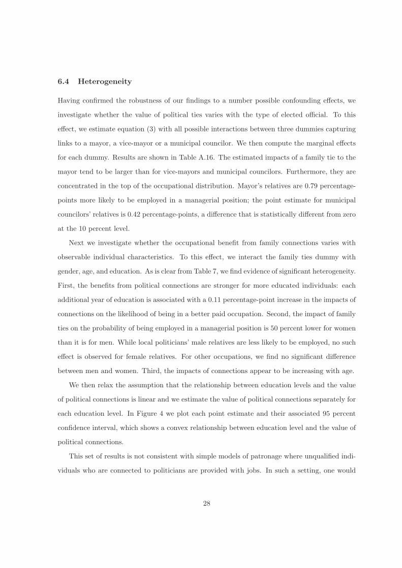
Results are consistent with strong positive impacts of political connections on the probability
of being employed in better-paid occupations (Table 2). The RDD estimate obtained with the
optimal bandwidth suggests that connections increase the likelihood of being employed in either
a professional or a managerial role by 7.42 percentage-points. Similarly, individuals connected to
current office-holders appear to experience a 1.25 percentage-points increase in the probability
of being employed in a managerial role. The point estimate represents 51 percent of the control
group mean. At the bottom of the distribution, family ties do no appear to affect the likelihood
of being employed. The point estimates decrease as the bandwidth increases. For example
with the bandwidth set at half the optimal bandwidth, connections appear to lead to a 1.67
percentage point increase in the probability of being employed in a managerial position. With
twice the optimal bandwidth, the point estimates correspond to 1.24 percentage point increase.
As discussed in the Introduction, we argue that in this particular context the RDD point
estimates combine both the benefits from connections to current office-holders and the cost
associated with being related to a candidate who lost which would explain the large point
in 27.5 percent of the municipalities in our sample. Comparing municipalities with and without close electionswe find that there is no statistically significant difference in terms of poverty incidence, of the number of timesthe incumbent’s family has been in office and of per capita fiscal transfers from the central government. Thereis some evidence that municipalities with close elections are slightly less populous (significant at the five percentlevel) but once we regress a dummy equal to one if either the mayoral or the vice-mayoral election was close in2007 on the set of four control variables, we are unable to reject the null of no effect for any of the coefficient.The F-stat for the regression is 1.95 (p-value .114).
18This is implemented in Stata using the rd command developed by Nichols (2011). It estimates local linearregressions with a triangle kernel.
14

estimates obtained.19 Indeed, individuals connected to candidates who were narrowly defeated
in the 2007 elections might suffer from their connections. We present four distinct pieces of
evidence consistent with this interpretation. First, we plot local polynomial regressions of the
probability of being employed in the best-paying occupation on their relatives’ vote share in
the 2007 elections (Figure 1). While the estimated probability is more or less stable at three
percent for individuals connected to losing candidates, starting at around 10 percentage-points,
the probability drops drastically and reaches about two percent for individuals connected to
politicians who were very narrowly defeated.
Second, to check that is not a general pattern of close elections, we also run some placebo
tests and plot local polynomial regressions of the probability of being employed in the best-
paying occupation on their relatives’ vote share in the 2010 elections; that is after the data were
collected. Not only there is no evidence of a drop for individuals connected to close losers, but
there is also no evidence of discontinuity in the probability of being employed as a manager at
the threshold (Figure 2).
Third, we compare individuals connected to unsuccessful candidates in the 2007 elections
and in the 2010 elections (but who did not run in 2007) and plot local polynomial regressions
of the probability of being employed in the best-paying occupation on their relatives’ vote
share (Figure A.1). For individuals connected to candidates who lost by a margin of less than
five percentage-points, the probability of being employed as a manager is noticeably lower for
individuals connected to 2007 candidates than for individuals connected to 2010 candidates. To
test this more formally, we restrict the sample to individuals connected to losing candidates
in either the 2007 or in the 2010 elections (but who did not run in 2007) and regress the
probability of being employed in the best-paying occupation on a dummy equal to one if the
individual is connected to a losing candidate in 2007. We are able to reject the null of no effect
for the sample of individuals connected to candidates who lost by less than five percentage-points
but not for individuals connected to candidates who lost by larger margins (Figure A.2). As
19Interpreting the RDD results could face additional challenges. First, the incentives of politicians who werenarrowly elected might differ from those who were elected with wider margins (Vyborny and Haseeb 2013).Second, there is also some debates in the literature as to whether close elections are indeed random (Caugheyand Sekhon 2011, Eggers, Folke, Fowler, Hainmueller, Hall and Snyder 2013).
15

discussed above, this is consistent with a theory of political control of the bureaucracy whereby
incumbents attempt to staff the bureaucracy with individuals whose incentives are aligned with
their own electoral objectives.20 Data constraints prevent us from testing this directly.
Fourth, if potential punishment explains the size of the RDD estimates, we would expect
them to be larger in municipalities where the incumbent lost than in municipalities where the
incumbent managed to get re-elected. This is what we find (Table A.4). In municipalities where
the incumbent lost, the RDD estimate obtained with the optimal bandwidth suggests that
connections increase the likelihood of being employed as a manager increases by 2.45 percentage
points (significant at the five percent level).21 In municipalities where the incumbent won, the
point-estimate drops to 0.44 percentage-points and we are unable to reject the null that it is
different from zero at the usual levels of statistical significance.
Finally, in light of common concerns of manipulation around the threshold, we carry out
standard balance tests, results of which are available in Column 1 of Table 3. Individuals on
the right side of the threshold have .68 more years of education and 38 percent more relatives
than individuals on the left side of the threshold. This has implications for the way the test
developed by McCrary (2008) needs to be interpreted in our context. Indeed, we use data from
the top two candidates in the mayoral and vice-mayoral elections and, by construction, for each
candidate who managed to get elected with vote margin x there is another candidate that lost
with vote margin −x ; implying that the underlying density is smooth. However, in the case
at hand, the test implicitly weights each candidate by the number of relatives. The McCrary
statistics is .655 with a standard error of .044 which lead us to reject the null. We argue that
this driven by differences in the number of relatives candidates have.
20An alternative view is that incumbents are sending a signal to potential challengers: an unsuccessful bidfor office will induce cost on the candidate’s relatives. If this second interpretation is correct then we wouldexpect individuals connected to politicians in opposition to suffer from their connections across a broad range ofoutcomes; not simply in terms of occupation. This is left for future research.
21It is important to note that this is not merely a short-run effect as most of the data were collected between18 and 30 months after the mayors elected in 2007 assumed office.
16

5 Alternative estimation strategy
In this section we propose an alternative estimation strategy that seeks to address the possible
interpretation challenges of the regression discontinuity approach applied to our data. Our aim
is to obtain credible estimates of the causal effect of political connections on occupation in a way
that distinguishes between the cost of losing an election and the benefit of winning one. We take
a step-by-step approach, discussing how data constraints and unobserved heterogeneity combine
to make the estimation of the value of political connections challenging. We also discuss how
we test for heterogeneous effects.
5.1 The benefits of political connections
In order to deal with unobserved heterogeneity, researchers attempting to provide credible es-
timates of the value of political connections need to identify a valid control group. We present
several approaches to identify a control group and discuss their relative advantages and draw-
backs. Our objective is to measure the benefits of political connections in a way that nets out
the possible cost of being connected to someone who just lost an election.
In most contexts, since data on connections to unsuccessful candidates tend not to be avail-
able, researchers are only able to compare politically connected individuals to individuals ran-
domly drawn from the population. To allow comparison with this literature, we start by es-
timating the value of political connections by regressing the outcome variable on a dummy
capturing links to elected local officials, plus individual controls. Specifically we estimate a
linear probability model of the form:
Yijt = αCijt + βXijt + vjt + uijt (2)
where Yijt is a measure of occupational choice for individual i in municipality j at the time of the
survey t, α is the parameter of interest, Cijt is a dummy variable that equals one if individual i
is related to an elected official in office in municipality j at time t, Xijt is a vector of observable
individual characteristics, vjt is an unobservable affecting all individuals in municipality j at
time t and uijt is an idiosyncratic error term. We introduce the time subscript since, as opposed
17
to the RD discussion, we use candidates across two electoral cycles. Occupational choice might
be correlated within provinces and we cluster standard errors at the provincial level.22
We estimate equation (2) in three different ways. We begin by including only municipal fixed-
effects. Then, we add individual controls Xijt for age, gender and, educational achievements. In
the third regression, we also control for i’s marital status, relationship to the household head,
history of displacement, and we include dummies for the month*year in which the interview
took place. Since we have a large number of observations, we include a full set of dummies for
each distinct value of each control variable.
While this approach has been used in the literature (e.g., Caeyers and Dercon (2012)), it
remains vulnerable to the presence of unobserved heterogeneity correlated with political con-
nections Cijt. To make this explicit, let us decompose uijt into three components:
uijt = μij + ηij + eijt
where eijt is a pure random term with E[eijtCijt] = 0. Let μij be the unobserved heterogeneity
associated with being related to someone who ran at least once in a local election. There are
good reasons to expect E[μij |Cijt = 1] > E[μij |Cijt = 0]. For instance, a higher social standing
makes it more likely that an individual is related to the local political elite, but also that he
or she has a better occupation. Similarly, let ηij be the additional unobserved heterogeneity
associated with being connected to a candidate who has won a local election at least once. We
expect E[ηij |Cijt = 1] > E[ηij |Cijt = 0]: on average, individuals with characteristics that make
them more likely to be related to a successful politician also have, other things being equal,
a social standing correlated with a better occupation. To the extent that E[μijCijt] > 0 and
E[ηijCijt] > 0, we expect an upward bias in estimates of α that are obtained by estimating
equation (2) on the entire population. If we can control for μij and ηij , α then captures the
effect of being related to an elected official currently in office, net of any correlation between
22The sample includes data from more than 60 provinces so we are not concerned about bias in our standarderrors as a result of having too few clusters (Cameron, Gelbach and Miller 2008). We also show that our resultsare similar if we cluster standard errors either at the municipal-level (Table A.19) or along both month×year andprovince, using the two-way clustering method developed Cameron, Gelbach and Miller (2011) (Table A.20).
18

social status and local politicians, successful or otherwise.
Control group I: Relatives of unsuccessful 2007 candidates As a first step in controlling
for unobserved heterogeneity, we estimate equation (2) on the restricted sample of all individuals
related to local politicians who ran in the 2007 elections. In this approach individuals related to
unsuccessful politicians serve as controls for individuals related to successful politicians. This is
similar to the RDD set-up presented above but all individuals are weighted equally, irrespective
of their relatives’ vote share in the past election. The purpose of this approach is to net out
unobserved heterogeneity μij . It delivers an unbiased estimate of α provided that E[ηijCijt] = 0.
Comparing to the α̂ obtained from (2) using the total population as control group yields an
estimate of the bias:
μ ≡ E[μij |Cijt = 1]− E[μij |Cijt = 0]
Control group II: Relatives of 2010 candidates Even in situations where E[ηijCijt] = 0,
using control group I to estimate the benefits of connections is vulnerable to one possible weak-
ness identified above. Imagine that relatives of an unsuccessful opponent in the last election are
punished by the successfully elected politician, and further imagine that this punishment trans-
lates in a lower occupation. In this case, the difference in occupation level Yijt between relatives
of successful and unsuccessful candidates in the last election overestimates α since it includes
the value of the punishment. This is only a source of bias if we think of the counterfactual as
the situation where none of individual i’s relatives had ran for office. Alternatively, if we think
of the counterfactual as the situation where the relative had ran but lost then the punishment
is part of what we are trying to estimate. We argue that being able to separately identify the
costs and benefits leads to a more precise interpretation of our findings.
One possible solution is to use as controls the relatives of politicians who ran in an election
taking place after survey time t, but who did not run in elections that took place before time t.
By construction, these politicians – and their relatives – cannot be punished at t for opposing the
currently elected official after t. To the best of our knowledge this is the first time this approach is
being used. Based on this idea, we estimate equation (2) on the sample of individuals connected
19

to either successful candidates in the 2007 elections, or to candidates in the 2010 elections who
did not run in 2007. This provides an estimate of α that nets out both μij and the punishment
meted out on unsuccessful opponents. Comparing it to the α̂ obtained using control group I
yields an estimate of the punishment effect. Next, we discuss the method that allows us to also
control for ηij .
Control group III: Relatives of successful 2010 candidates To control for both μij
and ηij while netting out possible punishments, we estimate equation (2) using a third control
group that only includes relatives of successful 2010 candidates who did not run for election in
2007. This control group minimizes sources of bias and should arguably yield the most accurate
estimate of α.23 But because it is the most restrictive, it also results in the smallest number of
control observations – and thus to a possible loss of power. To the best of our knowledge, this
is the first time this estimation strategy is being used to estimate the value of being connected
to an elected official for an individual.24
We report estimates using all three control groups. Comparison of α̂ estimates obtained with
control groups I and II provides an estimate of the punishment bias that can arise when using
a control group I approach. Comparison between estimates of α obtained with control groups
II and III provides an estimate of the bias:
η ≡ E[ηij |Cijt = 1]− E[ηij |Cijt = 0]
Control groups II and, especially, III are a marked improvement upon what the literature
has been able to use until now. We are able to use these control groups for several reasons.
First, we infer links from information about names, not from self-reported data. Control groups
II and III could not be constructed from self-reported measures of political connections: how
could respondents be asked about their connections to yet-to-be-revealed candidates? Second,
23Of course, the maintained assumption here is that the pool of candidates is comparable across the two electoralcycles. We are unable to completely rule out slight differences between the groups.
24Implicitly, this method is used in the literature on the impacts of political connections for firms. Researchersoften have access to panel data and can thus compare, within the set of firms that are politically connected atsome point in their sample years, firms that are connected at time t and those are not.
20

using names to infer family connections could be problematic in many countries but, for reasons
discussed in Section 3.2, in the Philippines names are particularly informative about family
ties. Finally, we have a very large sample and there is ample turnover of local politicians from
one election to the next. Had the sample been smaller and turnover less frequent, control and
treatment groups would have been too small to estimate α.
To better explain how the control groups are generated we now provide an example from the
municipality of Aguilar in the province of Pangasinan. In the 2007 mayoral election, candidate
Evangelista defeated candidate Zamuco for the position of mayor. In our set-up, individuals
related to Evangelista are classified as being connected to the current office-holder and all indi-
viduals related to candidate Zamuco belong to control group I. In the 2010 election, candidate
Evangelista ran against three candidates: De Los Santos, Sagles and Ballesteros. The latter
won the election. Control group II consists of individuals related to one of the three opponents
(Ballesteros, De Los Santos and Sagles). Control group III is made of individuals related to
Ballesteros.
Coming back to the descriptive statistics presented above, Columns 3-5 of Table 1 suggests
that a non-negligible share of the difference between individuals related to office holders and
the rest of the population may be due to unobserved heterogeneity correlated with political
connections: among individuals related to successful candidates in the 2010 elections who did
not run in 2007, 2.4 percent are employed in a managerial role, which is 20 percent more than
in the general population.
Before proceeding further, we now report balance tests for our three control groups. Results
are available in Columns 2-4 of Table 3. Overall, it appears that for the two key variables,
years of education and network size, the gap between elected officials’ relatives and the control
groups is about half for control group than what it is when using the RDD approach. This
reinforces our confidence that using relative of future winners as a control group is a valid
strategy. In the analysis below, we use two strategies to deal with this lack of balance. We start
by flexibly controlling for all variables and include a full set of dummies for each distinct value
of each control variable. We also present robustness checks where all the key variables are fully
saturated at the municipal-level. This will greatly reduce the risk that our results are driven by
21

lack of balance along observables.
5.2 Heterogeneity
We investigate whether the value of political connections varies with the rank of the local
politician to whom the individual is related. To this effect, we estimate equation (2) replacing
Cij with all possible interactions of three dummy variables capturing family ties to the mayor,
the vice-mayor, and municipal councilors and the associated marginal effects. We also test
whether the impact of political connections varies across individuals in a systematical way. More
specifically, we test for heterogenous effects along three characteristics Zpij – gender, education
and age – estimating equations of the form:
Yijt = αCijt + βXijt +3∑
p=1
(δpCijt(Zpij − Z̄p) + γpZ
pij) + vjt + uijt (3)
In the interaction term the Zpij variables are demeaned so that α still measures the average
treatment effect.
We also investigate heterogeneity at the municipal level. We expect that the economic
and political environment in the municipality influences the incentives and constraints that
politicians face to reward their relatives (Weitz-Shapiro 2012). To implement this idea, we
estimate a model of the form:
Yijt = αCijt + βXijt +P∑
p=1
δpCijt ∗ (Zpj − Z̄p) + vjt + uijt (4)
where Zpj is a relevant characteristic of the municipality. We do not control for Zp
j directly since
all regressions include municipal fixed-effects.
6 Econometric results
6.1 Main results
We begin by reporting naive OLS estimates using the full sample. Results indicate that individ-
uals connected to politicians in office are more likely to be employed in better paying occupations
22

(Table 4). For example, a randomly selected individual related to an elected local official is 1.45
percentage points more likely to be employed in a managerial role than the average citizen. This
represents an increase of about 70 percent of the mean.
As shown in Panels A and B of Table 4, a large share of this difference can be attributed
to observable characteristics. Depending on the outcome of interest, the inclusion of additional
controls reduces point estimates by 0.5-0.75 percentage points. For example, when we control
for age, gender, and education levels, the point estimates on the impact of connections on the
probability of being employed in a managerial role drops to 0.75 percentage-points. Adding
further controls does not affect the point estimates.
As explained in Section 5, we now compare these results to those obtained using different
control groups I, II and III. When we use control group I – i.e., the relatives of unsuccessful 2007
candidates – to net out unobserved heterogeneity μij , we obtain qualitatively similar results to
Table 4. A point made clearer by the comparison of the top left and top right corners of Figure
3. But point estimates are lower than the ones obtained on the full sample, a finding consistent
with the argument that bias μ is positive: depending on the outcome of interest, point estimates
fall by 29 to 40 percent (Panels B of Table 4 and Panel A of Table 5). For example, political
family ties are now associated with a 0.5 percentage-point increase in the probability of being
employed in a managerial role. Additional results are available in Table A.5.
Next we use control group II, in which the relatives of 2010 candidates who did not run in
2007 are compared to those of successful 2007 candidates (Panel B of Table 5). The purpose
is to net out μij and to avoid including in the estimate of political connections the potential
cost suffered by individuals connected to unsuccessful candidates. Results, shown in the bottom
left corner Figure 3 and in Panel B of Table 5, continue to associate family ties to elected
officials with better paid occupations. Additional results are available in Table A.6. As a
point of comparison, we also estimate the regressions on the sample of individuals connected to
unsuccessful candidates in 2010 who did not run in 2007, and find similar results (Table A.7).
Finally, we further restrict the control group to those individuals connected to successful
candidates in the 2010 elections but who did not run in 2007 to net out both μij and ηij . This
is control group III. Results, presented in the bottom right corner of Figure 3 and in Panel C
23

of Table 5, confirm that individuals connected to currently elected local officials are more likely
to be employed in better paid occupations. Although apparently small in magnitude, the effect
is economically significant: individuals connected to current office holders are 11 percent more
likely than individuals in the control group to be employed in either a professional or managerial
position and 22 percent more likely to be employed in a managerial position. Additional results
are available in Table A.8.
6.2 Discussion and interpretation
What do we learn from comparing estimates obtained using different control groups? First, as
anticipated, an upward bias seems to arise when we estimate the impacts of political connections
without adequately controlling for unobserved heterogeneity μ: point estimates obtained with
naive OLS are 50 to 70 percent higher than those obtained using control group I (Panels B of
Table 4 and A.5); similar results are obtained with control groups II and III, the latter also
controls for η.
Second, control groups I and III provide point estimates of similar order of magnitude. At
first glance, this suggests that η is close to zero and that the relatives of unsuccessful 2007
candidates do not suffer from their ties to an unlucky challenger. However, in a context where
the bureaucracy is politicized, such costs might only be suffered by a small number of individuals.
Indeed, incumbents might value loyalty, especially around election time, and might be reluctant
to staff the bureaucracy with individuals whose views and interests are antinomic to theirs.
Relative of close losers, i.e., relatives of candidates who almost won the 2007 elections, represent
a bigger threat than relatives of non-close losers and might be the ones suffering such costs. This
could explain why the point estimates obtained through RDD are higher than the ones obtained
with any of the three control groups and why the RDD estimates increase as the bandwidth
used decreases.
As point of further comparison with the RDD estimates provided above, we estimate equation
(2) on the sample of individuals related to candidates for either mayor or vice-mayor in the 2007
elections (Table A.9). The RDD estimates are 60 percent larger than the regression point
estimates on that subsample.
24

Based on the above evidence, we conclude that control group III provides the most credible
estimates of the benefits of family ties to elected local officials net of potential punishment.
Consequently, the robustness checks presented in the next sub-Section focus on that control
group.
We test for the impact of family ties on each occupation separately (Table A.10). We
only find significant effects for two occupations: local politicians’ relatives are less likely to be
employed as farmers (the second lowest paid occupation) and more likely to be employed in a
managerial position (the highest paid occupation). Since it is unlikely that farmers get assigned
to managerial posts, what our results suggest is that there is a shift of connected individuals
from lower to higher occupations across the whole spectrum, so that flows in and out of each
intermediate occupation cancel each other. This confirms that connected individuals benefit
from their ties to local politicians across the whole range of occupations.
In addition, we estimate equation (2) for each Y p (p = 2, . . . , 10) restricting the sample to
individuals for which Y p−1 = 1. Given that we can consider occupation choice as a sequential
decision, this is equivalent to estimating the conditional impacts of connections. This gives
us additional information about where in the distribution of occupations connections have an
impact.25 Results, available in Table A.11, suggest that, even the conditional estimates are
consistent with a positive impact of family connections on occupational choice. It is important
to note that those estimates need to be interpreted with caution as, for each value of p, the
probability of being included in the sample is correlated with the level of connections.
Before turning to robustness checks, we explore the effects of connections to local politicians
in office on three alternative measures of job quality. First, assuming that everyone employed
in occupation i earns the average daily wage in that occupation, we can put a monetary value
on the effect of political connections. Using control group III, we find that being connected to
a local politician in office leads to an increase of 2.27 Pesos per day (Column 1 of Table A.12).
25A simple example with two sequential decisions will highlight the differences between the conditional andunconditional estimates. Let’s assume that connections affect the probability of going through the first step, butconditional of having gone through the first step connections do not affect the probability of going through thesecond step. That is, assuming P (Y 1 = 1|C = 1) > P (Y 1 = 1|C = 0) and P (Y 2 = 1|Y 1 = 1, C = 0) = P (Y 2 =1|Y 1 = 1, C = 0), will lead to P (Y 2 = 1|C = 1) > P (Y 2 = 1|C = 0).
25

This corresponds to 1.84 percent of the mean control group III.26 Second, we get similar results
if use median wage rather than mean wage in each occupation (Column 2 of Table A.12). Third,
while we are unable to distinguish between the public and private sector in our data, we can
compute the percentage of individuals employed in occupation p who work in the public sector
from the nationally representative labor force surveys. We can then estimate the effect of being
connected to a politician in office on the probability of being employed in the public sector.
The point estimate is 0.204, which corresponds to 3.3 percent of the mean in control group III
(Column 3 of Table A.12).
6.3 Robustness checks
In this sub-section we verify the robustness of our results to various potential threats to our iden-
tification strategy and interpretation of the results. We ran a number of additional robustness
checks that are not discussed here but are included in the online appendix.
First, so far we have not allowed for the possibility that the size of the individual’s family
network could affect occupational choice. Results presented in Table 3 indicate that this might be
a concern and we take advantage of the data available to estimate equation (2) with a full set of
dummies for the number of individuals who share the individual’s last name in the municipality
and for the number of individuals who share the individual’s middle name in the municipality.
Results are robust to this change (Panel A of Table 6) which deals with concerns that we are
merely capture differences in network size. The full set of results are available in Table A.13.
Second, to reduce concerns about lack of balance, we introduced control variables flexibly
by generating a different dummy for each value of our control variables. Still, the model does
not allow for possible interactions between control variables such as age, education, and gender.
To verify whether this affected the results, we estimate an alternative model in which all the
age, gender and education variables and municipal dummies are all interacted with each other.
This leads us to estimating equation (2) with about 250,000 fixed-effects. This is akin to a very
26Gagliarducci and Manacorda (2014) estimates that, in Italy, having one more relative in office is associatedwith a 1.6 percent increase in private sector earnings. They identify connected individuals through shared lastname but only have data on the first three consonants of everyone last name and can only track family connectionson the father’s side. This generates both inclusion and exclusion errors in their connection measures.
26
restrictive matching estimator: identification comes from comparing connected individuals of
the same gender, age, and education living in the same municipality. Point estimates, reported
in Panel B of Table 6 are smaller but still economically and statistically significant. For example,
being connected to an elected official leads to a 0.36 percentage-points increase in the probability
of being employed in a managerial role. Further results are available in Table A.14.
Third, as indicated above, the main maintained assumption is that the pool of candidates
is comparable across the two electoral cycles. Violation of that assumption would imply that
our results might simply be capturing between candidates elected for the first time in 2007 and
candidates elected for the first time in 2010. While we are unable to test this directly, we we
estimate equation (2) on the sample of officials’ relatives in municipalities where the incumbent
mayor’s family was elected for either the first or second time in 2007. If our results were driven
by trends in the type of candidates running for office, we would expect officials’ relatives in
municipalities where the incumbent was elected for the second time in 2007 to be employed
in better-paying occupations than officials’ relatives in municipalities where the incumbent was
elected for the first time in 2007. This is not what we find. Results are available in Panel C of
Table 6.
Fourth, politicians are only able to stay in office for three consecutive terms, but political
families in some municipalities circumvent those term limits by having different members of the
same family take turns in office (Querubin 2011). In these municipalities, relatives of candidates
elected in 2010 might not be valid counterfactuals for current office holders.27 We re-estimate
equation (2) focusing on municipalities where the mayor’s family has been in office for three
terms or fewer (Panel D of Table 6).28 As expected the point estimates tend to be smaller, but
they remain economically and statistically significant and they tend to be located at the top of
the distribution of occupations. For example, in this subsample of municipalities, current office
holder’s relatives are 0.46 percentage-points more likely to be employed in a managerial role
and we are unable to reject the null hypothesis that the point estimates are equal to the ones
obtained on the full sample.
27This issue is discussed in detail in Ferraz and Finan (2011).28We re-estimate equation (2) focusing on municipalities where the mayor’s family has been in office fo two
terms or fewer (Panel B of Table A.15) and one term (Panel C of Table A.15).
27
6.4 Heterogeneity
Having confirmed the robustness of our findings to a number possible confounding effects, we
investigate whether the value of political ties varies with the type of elected official. To this
effect, we estimate equation (3) with all possible interactions between three dummies capturing
links to a mayor, a vice-mayor or a municipal councilor. We then compute the marginal effects
for each dummy. Results are shown in Table A.16. The estimated impacts of a family tie to the
mayor tend to be larger than for vice-mayors and municipal councilors. Furthermore, they are
concentrated in the top of the occupational distribution. Mayor’s relatives are 0.79 percentage-
points more likely to be employed in a managerial position; the point estimate for municipal
councilors’ relatives is 0.42 percentage-points, a difference that is statistically different from zero
at the 10 percent level.
Next we investigate whether the occupational benefit from family connections varies with
observable individual characteristics. To this effect, we interact the family ties dummy with
gender, age, and education. As is clear from Table 7, we find evidence of significant heterogeneity.
First, the benefits from political connections are stronger for more educated individuals: each
additional year of education is associated with a 0.11 percentage-point increase in the impacts of
connections on the likelihood of being in a better paid occupation. Second, the impact of family
ties on the probability of being employed in a managerial position is 50 percent lower for women
than it is for men. While local politicians’ male relatives are less likely to be employed, no such
effect is observed for female relatives. For other occupations, we find no significant difference
between men and women. Third, the impacts of connections appear to be increasing with age.
We then relax the assumption that the relationship between education levels and the value
of political connections is linear and we estimate the value of political connections separately for
each education level. In Figure 4 we plot each point estimate and their associated 95 percent
confidence interval, which shows a convex relationship between education level and the value of
political connections.
This set of results is not consistent with simple models of patronage where unqualified indi-
viduals who are connected to politicians are provided with jobs. In such a setting, one would
28

expect less educated and inexperienced individuals related to politicians to benefit from con-
nections the most. This is not what we find. While we do not have information about job
requirements, further analyses suggest that connected individuals tend to be better educated
than non-connected individuals employed in the same occupation. For example, among indi-
viduals who are employed in the best-paying occupation, 58.4 percent of individuals connected
to office-holders are college graduate while 53.3 percent of unconnected individuals are. The
corresponding figure for individuals in control group III is 54.8 percent.
Having examined individual-level heterogeneity, we turn to municipal-level heterogeneity and
investigate whether the value of political connections varies systematically with the municipal
environment. We first examine the role of per capita fiscal transfers to municipalities. We expect
that elected local politicians are better able to favor their relatives in municipalities that receive
larger transfers. As shown in Table 8, we find that, in municipalities with higher per capita
fiscal transfers, local politicians’ relatives are less likely to be employed but also more likely to
be employed in a managerial position.
We also investigate whether the value of political ties is stronger in municipalities where
the mayor’s family has been in office longer. Presumably, more entrenched incumbents are in
a better position to favor their relatives. This is indeed what we find – see Table 8. We also
find that the value of connections is lower in municipalities where a larger number of municipal
councilors did not run on the mayor’s ticket. This could indicate that municipal councils exert a
modicum of accountability check. To shed further light on this, we look separately at the effects
on individual connected to the mayor, vice-mayor, and municipal councilors. Results, shown in
Table A.17, indicate that the temporising effects of politically divided municipal councils on the
benefits of political connections are concentrated on the relatives of the mayor.
Finally, in some municipalities members of the same family compete against each other in
mayoral elections. In those municipalities our measure of connections likely does not capture
the relevant ties to elected officials and as such, we would expect our estimated coefficients to
be smaller there. As a result, we estimate equation (2) and interact our measure of connections
to elected officials with a dummy indicating whether two members of the same family ran
against each other during the 2007 mayoral elections. The effect is concentrated in municipalities
29

without within-family feuds in the 2007 mayoral elections (Table A.18). This does not imply
that connections are not important in those municipalities but, more likely, that our measure of
connections is not capturing the relevant ties in this specific context.
7 Conclusion
In this paper, we have provided evidence that family ties to a locally elected politician are as-
sociated with a better paid occupation. We argue that this association is causal.29 In addition
to numerous control variables, we have dealt with unobserved heterogeneity by using a variety
of control groups, including individuals related to candidates elected in subsequent elections.
The effects of political connections on better paid occupation that we find are economically and
statistically significant, and they are robust to controlling for a number of individual character-
istics, and to using many alternative specifications. In addition, we are able to identify a cost
of being related to an unsuccessful candidate who narrowly missed winning.
Our results have a number of implications and suggest some ideas for further research. First,
while we are unable to test this directly, we interpret our findings that close losers’ relatives suffer
from their connections as consistent with models of political control of the bureaucracy. This
is in line with the argument that incumbents value loyalty and might be reluctant to staff the
bureaucracy with individuals whose views and interests are incompatible with theirs. They
attempt to staff the bureaucracy with individuals whose incentives are aligned with their own
electoral objectives. Second, this could explain why the returns to connections increase with
education levels as politicians provide jobs to their most educated relatives as they are the
most capable of steering the bureaucracy. Further, this set of result is not consistent with
a view that the effects are purely driven by elected officials’ altruistic motives towards their
relatives. Third, in some contexts, estimates of the value of political connections obtained with
regression discontinuity designs potentially include the cost of being connected to an unsuccessful
candidate. Conditioning on close elections changes the nature of the parameter being estimated.
29We recognize that we are presenting estimates of the value of political connections in the short run. We willattempt to establish the dynamics of impacts in future research.
30

A question that remains unaddressed is whether or not the tendency for individuals related to
office-holders to be employed in better-paying occupations affects the way services are delivered
at the local level. Due to data constraints, we attempt to shed some light on this by correlating
municipal-level measures of the extent to which political connections distort local labor mar-
kets with the quality of health service delivery, which have been devolved to the municipal-level
(Capuno 2009, Khemani 2013).30 We use the difference in the probability of being employed
as a manager between individuals related to a politician in office between 2007 and 2010 and
individuals related to a politician that ran either in the 2007 or 2010 municipal elections as a
measure of distortion and find that an increase in the level of distortions is associated with an
increase in the percentage of kids under the age of 6 that are underweight (Panel A of Table
9). The correlation is robust to controlling for a number of municipal characteristics, includ-
ing poverty incidence, average education levels, gini and incumbent vote share in the previous
election. Interestingly, once we focus on education, a sector which has not been devolved to the
municipal-level, we find no correlation between those outcomes and labor market distortions as-
sociated with political connections (Panels B-E of Table 9). While we are unable to make causal
claims based on those results, they suggest that politicians’ ability to help their relatives secure
better-paying occupations affect the way services are delivered by the municipal bureaucracy.
30Given that the analysis is carried out at the municipal-level, we do not use the sample split approach for thisset of regressions to avoid a strong loss in statistical power.
31

References
Alesina, Alberto and Paola Giuliano, “Family Ties,” in Philippine Aghion and StevenDurlauf, eds., Handbook of Economic Growth, North Holland, 2013.
Angelucci, Manuela, Giacomo De Giorgi, and Imran Rasul, “Resource Pooling WithinFamily Networks: Insurance and Investment,” University College London, mimeo, 2012.
, , Marcos Rangel, and Imran Rasul, “Family Networks and School Enrolment:Evidence from a Randomized Social Experiment,” Journal of Public Economics, 2010, 94(3-4), 197 – 221.
Besley, Timothy, “Political Selection,” The Journal of Economic Perspectives, 2005, 19 (3),43–60.
, Rohini Pande, and Vijayendra Rao, “Just Rewards? Local Politics and PublicResource Allocation in South India,” World Bank Economic Review, 2012, 26 (2), 191–216.
, Torsten Persson, and David Sturm, “Political Competition, Policy and Growth:Theory and Evidence from the US,” Review of Economic Studies, 2010, 77, 1329–1352.
Blanes i Vidal, Jordi, Mirko Draca, and Christian Fons-Rosen, “Revolving Door Lob-byists,” American Economic Review, 2012, 102 (7), 3731–48.
Caeyers, Bet and Stefan Dercon, “Political Connections and Social Networks in TargetedTransfer Programmes: Evidence from Rural Ethiopia,” Economic Development and Cul-tural Change, 2012, 60 (4), 639–675.
Cameron, Colin, Jonah Gelbach, and Douglas Miller, “Bootstrap-based improvementsfor inference with clustered errors,” Review of Economics and Statistics, 2008, 90 (3), 414–427.
, , and , “Robust Inference with Multiway Clustering,” Journal of Business andEconomic Statistics, 2011, 29 (2), 238–249.
Capuno, Joseph, “A Case Study of the Decentralization of Health and Education Services inthe Philippines,” HDN Discussion Paper Series No. 3, 2009.
Casey, Katherine, Rachel Glennerster, and Edward Miguel, “Reshaping Institutions:Evidence on Aid Impacts Using a Pre-Analysis Plan,” Quarterly Journal of Economics,2012, 127 (4), 1755–1812.
Caughey, Devin and Jasjeet S. Sekhon, “Elections and the Regression Discontinuity DesignLessons from Close U.S. House Races 1942 2008,” Political Analysis, 2011, 19 (4), 385–408.
Cingano, Federico and Paolo Pinotti, “Politicians at Work: The Private Returns and SocialCosts of Political Connections,” Journal of the European Economic Association, 2013, 11(2), 433–465.
Clark, Gregory, The Son Also Rises: Surnames and the History of Social Mobility, NewJersey, USA: Princeton University Press, 2014.
32

Comola, Margherita and Marcel Fafchamps, “Testing Unilateral and Bilateral Link For-mation,” Economic Journal, forthcoming.
Coronel, Sheila, “Cavite - The Killing Fields of Commerce,” in “Boss - Five Case Studes ofLocal Politics in the Philippines,” Philippine Center for Investigative Journalism, 1995.
Cruz, Cesi and Christina Schneider, “The (Unintended) Electoral Effects of MultilateralAid Projects,” University of California - San Diego, mimeo, 2013.
Cullinane, Michael, “Patron as Client: Warlord Politics and the Duranos of Danao,” inAlfred McCoy, ed., An Anarchy of Families: State & Family in the Philippines, Madison,WI: University of Wisconsin Press, 2009, pp. 163–241.
Deaton, Angus, “Your Wolf is Interfering with my T-value!,” Royal Economic Society Newslet-ter, 2012, 159 (4).
Dios, Emmanuel De, “Local Politics and Local Economy,” in Arsenio M. Balisacan andHall Hill, eds., The Dynamics of Regional Development, Quezon City: Ateneo de ManilaUniversity Press, 2007.
Eggers, Andrew and Jens Hainmueller, “MPs for Sale? Returns to Office in PostwarBritish Politics,” American Political Science Review, 2009, 103 (4), 513–533.
, Olle Folke, Anthony Fowler, Jens Hainmueller, Andrew Hall, and James Sny-der, “Design for Estimating Electoral Effects: New Evidence from over 40,000 Close Races,”mimeo, 2013.
Einav, Liran and Jonathan Levin, “The Data Revolution and Economic Analysis,” NBERWorking Paper 19035, 2013.
Faccio, Mara, “Politically Connected Firms,” American Economic Review, 2006, 96 (1), 369–386.
Fernandez, Luisa, “Design and Implementation Features of the National Household TargetingSystem in the Philippines,” World Bank - Philippines Social Protection Note No 5, 2012.
Ferraz, Claudio and Frederico Finan, “Electoral Accountability and Corruption: Evidencefrom the Audits of Local Governments,” American Economic Review, 2011, 101 (4), 1274–1311.
Fisman, Ray, Florian Schulz, and Vikrant Vig, “The Private Returns to Public Office,”Journal of Political Economy, forthcoming.
Fisman, Raymond, “Estimating the Value of Political Connections,” American EconomicReview, 2001, 91 (4), 1095–1102.
Fukuyama, Francis, The Origins of political order: from prehuman times to the French revo-lution, New York, NY: Farrar, Straus and Giroux, 2011.
Gagliarducci, Stefano and Marco Manacorda, “Politics in the Family: Nepotism and theHiring Decisions of Italian Firms,” mimeo, 2014.
33

Gealogo, Francis Alvarez, “Looking for Claveria’s Children: Church, State, Power, and theIndividual in Philippine Naming Systems during the Late Nineteenth Century,” in ZhengYangwen and Charles J-H MacDonald, eds., Personal Names in Asia. History, Culture andHistory, Singapore: NUS Press, 2010, pp. 37–51.
Glaeser, E., “Researcher Incentives and Empirical Methods,” Harvard Institute of EconomicResearch, Discussion Paper Number 2122, 2006.
Guell, Maia, Jos V. Rodriguez Mora, and Christopher I. Telmer, “The InformationalContent of Surnames, the Evolution of Intergenerational Mobility and Assortative Mat-ing*,” The Review of Economic Studies, 2014.
Hale, Henry, “Correlates of Clientelism: Political Economy, Politicized Ethnicity, and Post-Communist Transition,” in Herbert Kitschelt and Steven Wilkinson, eds., Patrons, Clients,and Policies. Patterns of Democratic Accountability and Political Competition, CambridgeUniversity Press, 2007.
Hodder, Rupert, “Political Interference in the Philippine Civil Service,” Environment andPlanning C: Government and Policy, 2009, 27 (5), 766–782.
Hsieh, Chang-Tai, Edward Miguel, Daniel Ortega, and Francisco Rodriguez, “ThePrice of Political Opposition: Evidence from Venezuela’s Maisanta,” American EconomicJournal: Applied Economics, 2011, 3 (2), 196–214.
Human Rights Watch, They Own the People. The Ampatuans, State-Backed Militias, andKillings in the Southern Philippines, New York, NY: Human Rights Watch, 2010.
Humphreys, Macartan, Raul Sanchez de la Sierra, and Peter van der Windt, “Fish-ing, Commitment, and Communication: A Proposal for Comprehensive Nonbinding Re-search Registration,” Political Analysis, 2013, 21 (1), 1–20.
Imbens, Guido and Karthik Kalyanaraman, “Optimal Bandwidth Choice for the Regres-sion Discontinuity Design,” Review of Economic Studies, 2012, 79 (3), 933–959.
Imbens, Guido W. and Thomas Lemieux, “Regression Discontinuity Designs: A Guide toPractice,” Journal of Econometrics, 2008, 142 (2), 615–635.
Iyer, Lakshmi and Anandi Mani, “Traveling Agents: Political Change and BureaucraticTurnover in India,” Review of Economics and Statistics, 2012, 94 (3), 723–739.
Khemani, Stuti, “Buying Votes vs. Supplying Public Services: Political Incentives to Under-Invest in Pro-Poor Policies,” World Bank Policy Research Working Paper 6339, 2013.
Khwaja, Asim Ijaz and Atif Mian, “Do Lenders Favor Politically Connected Firms? RentProvision in an Emerging Financial Market,” Quarterly Journal of Economics, 2005, 120(4), 1371–1411.
Labonne, Julien, “Local Political Business Cycles. Evidence from Philippine Municipalities,”University of Oxford, mimeo, 2013.
34

Lande, Carl, Leaders, Factions and Parties: The Structure of Philippines Politics, Yale Uni-versity Southeast Asia Studies, New Haven CO, 1965.
Leamer, Edward, Specification Searches. Ad Hoc Inference with Nonexperimental Data, NewYork, NY: Wiley, 1978.
, “Let’s Take the Con out of Econometrics,” American Economic Review, 1983, 73 (1),31–43.
Markussen, Thomas and Finn Tarp, “Political Connections and Land-Related Investmentin Rural Vietnam,” Journal of Development Economics, forthcoming.
McCoy, Alfred, “An Anarchy of Families: The Historiography of State and Family in thePhilippines,” in Alfred McCoy, ed., An Anarchy of Families: State & Family in the Philip-pines, Madison, WI: University of Wisconsin Press, 2009, pp. 1–32.
McCrary, Justin, “Manipulation of the Running Variable in the Regression DiscontinuityDesign: A Density Test,” Journal of Econometrics, 2008, 142.
Medina, Luis Fernando and Susan Stokes, “Monopoly and Monitoring: An Approach toPolitical Clientelism,” in Herbert Kitschelt and Steven Wilkinson, eds., Patrons, Clients,and Policies. Patterns of Democratic Accountability and Political Competition, CambridgeUniversity Press, 2007.
Nichols, Austin, “rd 2.0: Revised Stata module or regression discontinuity design,” 2011.
Querubin, Pablo, “Political Reform and Elite Persistence: Term Limits and Political Dynastiesin the Philippines,” mimeo, MIT, 2011.
, “Family and Politics: Dynastic Incumbency Advantage in the Philippines,” mimeo, NYU,2013.
and James Snyder, “The Control of Politicians in Normal Times and Times of Crisis:Wealth Accumulation by U.S. Congressmen, 1850-1880,” Quarterly Journal of PoliticalScience, 2013, 8, 409–450.
Scott, James, Seeing like a State: How Certain Schemes to Improve the Human ConditionHave Failed, New Haven, Conn.: Yale University Press, 1998.
Sidel, John, Capital, Coercion, and Crime: Bossism in the Philippines Contemporary Issuesin Asia and Pacific, Stanford, CA: Stanford University Press, 1999.
The Economist, A bridge too far? January 2014.
Tremewan, Christopher, The Political Economy of Social Control in Singapore, New York,USA: St Martin’s, 1994.
Vyborny, Kate and Muhammad Haseeb, “Patronage and Public Services: Evidence fromPunjab, Pakistan,” University of Oxford, mimeo, 2013.
35

Wallis, J.J., “The Concept of Systematic Corruption in American History,” in Edward Glaeserand Claudia Goldin, eds., Corruption and Reform: Lessons from America’s EconomicHistory, University of Chicago Press, 2006.
, Price Fishback, and Shawn Kantor, “Politics, Relief, and Reform. Roosevelt’s Effortsto Control Corruption and Political Manipulation during the New Deal,” in Edward Glaeserand Claudia Goldin, eds., Corruption and Reform: Lessons from America’s EconomicHistory, University of Chicago Press, 2006.
Wang, Shing-Yi, “Marriage Networks, Nepotism and Labor Market Outcomes in China,”American Economic Journal: Applied Economics, 2013, 5 (3), 91–112.
Weitz-Shapiro, Rebecca, “What Wins Votes: Why Some Politicians Opt Out of Clientelism,”American Journal of Political Science, 2012, 56 (3), 568–583.
Wilkinson, Steven, “Explaining Changing Patterns of Party-voter Linkages in India,” inHerbert Kitschelt and Steven Wilkinson, eds., Patrons, Clients, and Policies. Patternsof Democratic Accountability and Political Competition, Cambridge University Press, 2007.
36

.01
.02
.03
.04
.05
.06
Pr(
Man
ager
ial J
ob=
1)
-30 -15 0 15 30Vote Margin (2007 Elections)
Related to Losers Related to Winners95% Conf. Int.
Figure 1: Non-parametric estimates of the probability of being employed in a managerial position
-.05
0.0
5.1
.15
Pr(
Man
ager
ial J
ob=
1)
-30 -15 0 15 30Vote Margin (2010 Elections)
Related to Losers Related to Winners95% Conf. Int.
Figure 2: Non-parametric estimates of the probability of being employed in a managerial position
37

-.01
-.00
50
.005
.01
0 2 4 6 8 10
Full Sample
-.01
-.00
50
.005
.01
0 2 4 6 8 10
Control Group I
-.01
-.00
50
.005
.01
Bet
a
0 2 4 6 8 10Occupation
Control Group II-.
01-.
005
0.0
05.0
1B
eta
0 2 4 6 8 10Occupation
Control Group III
Point Estimates 95% Confidence Interval
Figure 3: Estimated effects of connections with various control groupsNotes: Results from municipal fixed-effects regressions. Control group I includes relatives of unsuccessfulcandidates in the 2007 elections, Control group II includes relatives of candidates in the 2010 electionswho did not run in 2007 and Control group III includes relatives of successful candidates in the 2010elections who did not run in 2007. All regressions include a full set of dummies for age, education leveland gender. The standard errors used to generate the 95% confidence intervals account for potentialcorrelation within province. Associated results are reported in Panel B of Tables 4 and A.5-A.8.
-.01
0.0
1.0
2.0
3B
eta
0 5 10 15Years of Education
95% Confidence Interval Point Estimates
Figure 4: Estimated effects of connections by education levels
38

Table 1: Descriptive statistics: Individual-level
Full Sample Connected Control GroupI II III
(1) (2) (3) (4) (5)
Occupation0 None 40.28 40.70 40.74 40.27 40.491 Laborers, Unskilled Workers 15.46 14.14 14.86 14.56 14.872 Farmers, Forestry Workers, Fishermen 28.80 26.08 27.25 28.64 28.253 Service, Shop, Market Sales Workers 5.06 5.53 5.45 5.12 4.774 Trades, Related workers 2.04 2.25 2.06 2.09 2.175 Plant, Machine Operators, Assemblers 1.46 1.45 1.48 1.47 1.466 Clerks 0.59 0.86 0.75 0.65 0.697 Technicians, Associate Professionals 0.60 0.73 0.72 0.68 0.668 Special Occupations 1.27 1.33 1.20 1.29 1.229 Professionals 2.41 3.67 3.08 2.89 3.0110 Officials, Managers, Supervisors 2.04 3.26 2.42 2.34 2.40
ControlsAge 39.26 40.16 39.77 39.46 39.66Education (years) 8.17 9.04 8.68 8.48 8.52Female 0.49 0.50 0.50 0.49 0.49
Observations 3,917,712 395,392 390,300 239,431 58,952
Notes: Control group I includes relatives of unsuccessful candidates in the 2007 elections, Control groupII includes relatives of candidates in the 2010 elections who did not run in 2007 and Control group IIIincludes relatives of successful candidates in the 2010 elections who did not run in 2007.
39
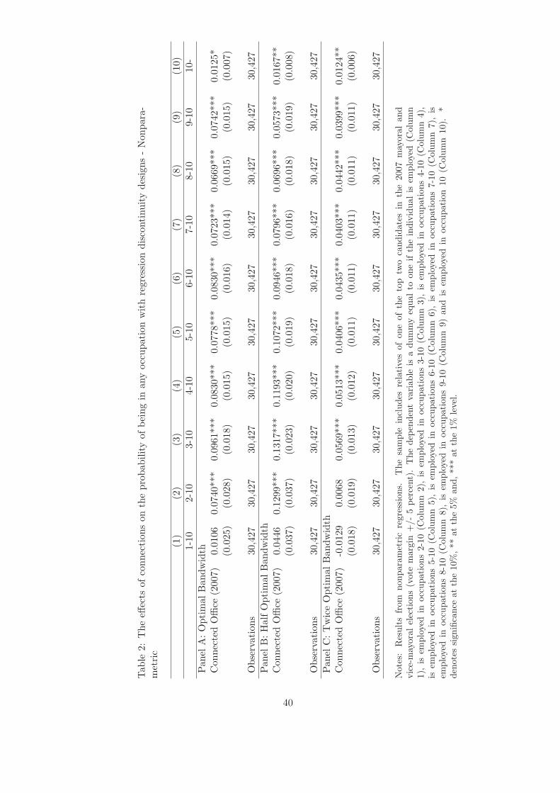
Tab
le2:
Theeff
ects
ofconnectionsontheprobabilityof
beingin
anyoccupationwithregressiondiscontinuitydesigns-Nonpara-
metric
(1)
(2)
(3)
(4)
(5)
(6)
(7)
(8)
(9)
(10)
1-10
2-10
3-10
4-10
5-10
6-10
7-10
8-10
9-10
10-
Pan
elA:OptimalBandwidth
ConnectedOffice
(2007)
0.0106
0.0740***
0.0961***
0.0830***
0.0778***
0.0830***
0.0723***
0.0669***
0.0742***
0.0125*
(0.025)
(0.028)
(0.018)
(0.015)
(0.015)
(0.016)
(0.014)
(0.015)
(0.015)
(0.007)
Observations
30,427
30,427
30,427
30,427
30,427
30,427
30,427
30,427
30,427
30,427
Pan
elB:HalfOptimalBandwidth
ConnectedOffice
(2007)
0.0446
0.1299***
0.1317***
0.1193***
0.1072***
0.0946***
0.0796***
0.0696***
0.0573***
0.0167**
(0.037)
(0.037)
(0.023)
(0.020)
(0.019)
(0.018)
(0.016)
(0.018)
(0.019)
(0.008)
Observations
30,427
30,427
30,427
30,427
30,427
30,427
30,427
30,427
30,427
30,427
Pan
elC:TwiceOptimalBandwidth
ConnectedOffice
(2007)
-0.0129
0.0068
0.0569***
0.0513***
0.0406***
0.0435***
0.0403***
0.0442***
0.0399***
0.0124**
(0.018)
(0.019)
(0.013)
(0.012)
(0.011)
(0.011)
(0.011)
(0.011)
(0.011)
(0.006)
Observations
30,427
30,427
30,427
30,427
30,427
30,427
30,427
30,427
30,427
30,427
Notes:
Resultsfrom
nonparametricregressions.
Thesample
includes
relativesofoneof
thetop
twocandidatesin
the2007mayoralan
dvice-mayoralelections(vote
margin
+/-5percent).Thedep
endentvariable
isadummyequalto
oneiftheindividualis
employed(C
olumn
1),
isem
ployedin
occupations2-10(C
olumn2),is
employedin
occupations3-10(C
olumn3),
isem
ployedin
occupations4-10(C
olumn4),
isem
ployedin
occupations5-10(C
olumn5),
isem
ployedin
occupations6-10(C
olumn6),
isem
ployed
inoccupations7-10(C
olumn7),
isem
ployedin
occupations8-10(C
olumn8),
isem
ployedin
occupations9-10(C
olumn9)andis
employedin
occupation10(C
olumn10).
*denotessignificance
atthe10%,**
atthe5%
and,***atthe1%
level.
40

Table 3: Balance Tests
RDD Control GroupI II III
(1) (2) (3) (4)
Panel A: AgeConnected Office (2007) 0.0014 0.0021*** 0.0026*** 0.0013
(0.025) (0.001) (0.001) (0.002)
Observations 30,427 786,436 635,432 454,889R-squared 0.001 0.001 0.001
Panel B: Education (years)Connected Office (2007) 0.6498*** 0.3245*** 0.4794*** 0.3600***
(0.174) (0.041) (0.043) (0.064)
Observations 30,427 786,436 635,432 454,889R-squared 0.137 0.144 0.134
Panel C: FemaleConnected Office (2007) -0.2358 0.0718 0.2804*** 0.2856***
(0.700) (0.048) (0.052) (0.073)
Observations 30,427 786,436 635,432 454,889R-squared 0.029 0.030 0.030
Panel D: Number of Relatives (log)Connected Office (2007) 0.3875*** 0.1627*** 0.2814*** 0.2099***
(0.059) (0.021) (0.029) (0.049)
Observations 30,427 786,436 635,432 454,889R-squared 0.219 0.224 0.236
Notes: This table reports various balance tests estimated on different samples either through RDD orOLS. In Column 1, the sample includes relatives of one of the top two candidates in the 2007 mayoraland vice-mayoral elections (vote margin +/- 5 percent) and the effects are estimated through RDD. InColumns 2-4, the dependent variable is regressed on a dummy equal to one if the respondent is related toa politician that was elected to office in 2007 and a full set of municipal dummies. In Column 2, officials’relatives are compared to relatives of unsuccessful candidates in the 2007 elections (Control Group I). InColumn 3, officials’ relatives are compared to relatives of candidates in the 2010 elections who did notrun in 2007 (Control Group II). In Column 4, officials’ relatives are compared to relatives of successfulcandidates in the 2010 elections who did not run in 2007. In Panel A, the dependent variable is age. InPanel B, the dependent variables is the number of years of educations. In Panel C, the dependent variableis a dummy equal to one if the respondent is female. In Panel D, the dependent variable is the log of thesum of the number of individuals who share the individual’s middle name in the municipality and of thenumber of individuals who share the individual’s middle name in the municipality. In Columns 2-4, thestandard errors (in parentheses) account for potential correlation within province. * denotes significanceat the 10%, ** at the 5% and, *** at the 1% level.
41

Tab
le4:Theeff
ects
ofconnectionsontheprobabilityof
beingin
anyoccupation-Fullsample
(1)
(2)
(3)
(4)
(5)
(6)
(7)
(8)
(9)
(10)
1-10
2-10
3-10
4-10
5-10
6-10
7-10
8-10
9-10
10-
Pan
elA:MunicipalFixed
Effects
ConnectedOffice
(2007)
-0.0041***
0.0049***
0.0415***
0.0377***
0.0355***
0.0348***
0.0322***
0.0307***
0.0280***
0.0145***
(0.002)
(0.002)
(0.002)
(0.002)
(0.002)
(0.002)
(0.002)
(0.002)
(0.002)
(0.001)
Observations
3,917,712
3,917,712
3,917,712
3,917,712
3,917,712
3,917,712
3,917,712
3,917,712
3,917,712
3,917,712
R-squared
0.022
0.052
0.037
0.026
0.023
0.023
0.022
0.022
0.014
0.010
Pan
elB:MunicipalFixed
Effects
andIndividualControls
(1)
ConnectedOffice
(2007)
-0.0075***
-0.0048***
0.0112***
0.0112***
0.0104***
0.0103***
0.0096***
0.0099***
0.0091***
0.0075***
(0.001)
(0.001)
(0.001)
(0.001)
(0.001)
(0.001)
(0.001)
(0.001)
(0.001)
(0.001)
Observations
3,917,706
3,917,706
3,917,706
3,917,706
3,917,706
3,917,706
3,917,706
3,917,706
3,917,706
3,917,706
R-squared
0.283
0.233
0.197
0.208
0.229
0.260
0.242
0.229
0.239
0.068
Pan
elC:MunicipalFixed
Effects
andIndividualControls
(2)
ConnectedOffice
(2007)
-0.002
-0.001
0.0124***
0.0121***
0.0109***
0.0107***
0.0100***
0.0103***
0.0094***
0.0076***
(0.001)
(0.001)
(0.001)
(0.001)
(0.001)
(0.001)
(0.001)
(0.001)
(0.001)
(0.001)
Observations
3,917,706
3,917,706
3,917,706
3,917,706
3,917,706
3,917,706
3,917,706
3,917,706
3,917,706
3,917,706
R-squared
0.347
0.275
0.200
0.211
0.231
0.261
0.243
0.230
0.240
0.069
Notes:
Resultsfrom
fixed
-effects
regressions.
Thedep
endentvariable
isadummyequalto
oneiftheindividualis
employed(C
olumn1),
isem
ployedin
occupations2-10(C
olumn2),isem
ployedin
occupations3-10(C
olumn3),isem
ployedin
occupations4-10(C
olumn4),isem
ployed
inoccupations5-10(C
olumn5),
isem
ployedin
occupations6-10(C
olumn6),
isem
ployedin
occupations7-10(C
olumn7),
isem
ployedin
occupations8-10(C
olumn8),
isem
ployedin
occupations9-10(C
olumn9)andis
employedin
occupation10(C
olumn10).
InPanelsB
and
C,allregressionsincludeafullsetofdummiesforage,
educationlevel
andgender.In
addition,in
Panel
C,regressionsincludeafullsetof
dummiesforrelationship
tothehousehold
head,maritalstatus,
month/yearoftheinterview,history
ofdisplacementan
dlength
ofstay
inthe
village.
Thestandard
errors
(inparentheses)accountforpotentialcorrelationwithin
province.*den
otessignificance
atthe10%,**
atthe5%
and,***atthe1%
level.
42

Tab
le5:
Theeff
ects
ofconnectionsontheprobabilityof
beingin
anyoccupation-Threecontrolgroups
(1)
(2)
(3)
(4)
(5)
(6)
(7)
(8)
(9)
(10)
1-10
2-10
3-10
4-10
5-10
6-10
7-10
8-10
9-10
10-
Pan
elA:ControlGroupI
ConnectedOffice
(2007)
0.001
0.001
0.0082***
0.0080***
0.0063***
0.0063***
0.0062***
0.0067***
0.0060***
0.0050***
(0.002)
(0.002)
(0.001)
(0.001)
(0.001)
(0.001)
(0.001)
(0.001)
(0.001)
(0.001)
Observations
785,692
785,692
785,692
785,692
785,692
785,692
785,692
785,692
785,692
785,692
R-squared
0.330
0.270
0.223
0.238
0.259
0.287
0.267
0.254
0.255
0.080
Pan
elB:ControlGroupII
ConnectedOffice
(2007)
-0.001
-0.001
0.0100***
0.0085***
0.0075***
0.0075***
0.0067***
0.0070***
0.0066***
0.0056***
(0.001)
(0.002)
(0.002)
(0.001)
(0.001)
(0.001)
(0.001)
(0.001)
(0.001)
(0.001)
Observations
634,823
634,823
634,823
634,823
634,823
634,823
634,823
634,823
634,823
634,823
R-squared
0.332
0.271
0.226
0.240
0.261
0.290
0.270
0.258
0.259
0.083
Pan
elC:ControlGroupIII
ConnectedOffice
(2007)
-0.002
-0.002
0.0085***
0.0060***
0.0062***
0.0066***
0.0062***
0.0065***
0.0061***
0.0054***
(0.003)
(0.003)
(0.003)
(0.002)
(0.002)
(0.002)
(0.002)
(0.002)
(0.002)
(0.001)
Observations
454,344
454,344
454,344
454,344
454,344
454,344
454,344
454,344
454,344
454,344
R-squared
0.331
0.271
0.232
0.246
0.268
0.297
0.277
0.264
0.264
0.088
Notes:
Resultsfrom
fixed
-effects
regressions.
Thedep
endentvariable
isadummyequalto
oneif
theindividualis
employed
(Column
1),
isem
ployedin
occupations2-10(C
olumn2),
isem
ployedin
occupations3-10(C
olumn3),
isem
ployed
inoccupations4-10(C
olumn4),
isem
ployed
inoccupations5-10(C
olumn
5),
isem
ployed
inoccupations6-10(C
olumn
6),
isem
ployed
inoccupations7-10(C
olumn
7),
isem
ployedin
occupations8-10(C
olumn8),
isem
ployedin
occupations9-10(C
olumn9)
andis
employedin
occupation10(C
olumn10).
All
regressionsincludeafullsetofdummiesforage,
educationlevel,gender,relationship
tothehousehold
head,maritalstatus,
month/yearofthe
interview,history
ofdisplacementan
dlength
ofstay
inthevillage.
Thestandard
errors
(inparentheses)accountforpotentialcorrelationwithin
province.*denotessignificance
atthe10%,**
atthe5%
and,***atthe1%
level.
43

Tab
le6:
RobustnessChecks
(1)
(2)
(3)
(4)
(5)
(6)
(7)
(8)
(9)
(10)
1-10
2-10
3-10
4-10
5-10
6-10
7-10
8-10
9-10
10-
Pan
elA:ControllingforNetwork
Size
ConnectedOffice
(2007)
-0.001
-0.002
0.0097***
0.0067***
0.0070***
0.0071***
0.0067***
0.0068***
0.0062***
0.0052***
(0.003)
(0.003)
(0.003)
(0.002)
(0.002)
(0.002)
(0.002)
(0.002)
(0.001)
(0.001)
R-squared
0.332
0.273
0.233
0.247
0.269
0.298
0.278
0.265
0.265
0.089
Pan
elB:Estim
ate
aSaturatedModel
ConnectedOffice
(2007)
-0.003
-0.000
0.0106***
0.0071***
0.0066***
0.0064***
0.0045**
0.0047**
0.0050***
0.0036**
(0.003)
(0.004)
(0.003)
(0.003)
(0.002)
(0.002)
(0.002)
(0.002)
(0.002)
(0.002)
R-squared
0.073
0.042
0.008
0.006
0.005
0.004
0.004
0.003
0.003
0.003
Pan
elC:First
term
vs.
Secondterm
Secondterm
0.019
0.019
-0.004
-0.003
-0.001
-0.006
-0.005
-0.006
-0.002
0.002
(0.012)
(0.017)
(0.004)
(0.004)
(0.004)
(0.004)
(0.004)
(0.004)
(0.003)
(0.003)
R-squared
0.322
0.251
0.220
0.235
0.257
0.285
0.263
0.249
0.252
0.082
Pan
elD:Municipalities
wheremayor’s
familyhasbeenin
office
threetimes
orless
ConnectedOffice
(2007)
-0.003
-0.002
0.0071**
0.003
0.0044**
0.0050***
0.0044**
0.0053***
0.0055***
0.0046***
(0.004)
(0.004)
(0.003)
(0.002)
(0.002)
(0.002)
(0.002)
(0.002)
(0.001)
(0.002)
R-squared
0.330
0.268
0.231
0.243
0.264
0.293
0.272
0.258
0.259
0.087
Notes:
Resultsfrom
fixed-effects
regressions.
n=
454,344(P
anelsA
andB),n=
170,030(P
anel
C)andn=
277,285(P
anel
D).Thedep
endent
variableisadummyequalto
oneiftheindividualisem
ployed(C
olumn1),isem
ployedin
occupations2-10(C
olumn2),isem
ployed
inoccupations
3-10(C
olumn3),is
employedin
occupations4-10(C
olumn4),
isem
ployedin
occupations5-10(C
olumn5),
isem
ployedin
occupations6-10
(Column6),isem
ployedin
occupations7-10(C
olumn7),isem
ployedin
occupations8-10(C
olumn8),isem
ployedin
occupations9-10(C
olumn
9)andisem
ployedin
occupation10(C
olumn10).
Allregressionsincludeafullsetofdummiesforage,
educationlevel,gender,forrelationship
tothehousehold
head,maritalstatus,
month/yearoftheinterview,history
ofdisplacementandlength
ofstay
inthevillage.
InPanel
A,
regressionsincludeafullof
setofdummiesforthenumber
ofindividualswhoshare
theindividual’smiddle
namein
themunicipality
andforthe
number
ofindividualswhoshare
theindividual’smiddle
namein
themunicipality.In
Pan
elB,regressionsincludedummiesforeach
interaction
oftheage,
education,gen
der
andmunicipaldummies.
InPan
elC,thesample
isrestricted
toindividualsconnectedto
electedofficialsin
2007in
municipalities
wheretheincu
mbentmayor
waselectedforthefirstorsecondtimein
2007.In
Panel
Dthesample
isrestricted
tomunicipalities
wheretheincu
mbentmayor’sfamilyhasbeenin
office
less
than4times.Thestandard
errors
(inparentheses)accountforpotentialcorrelation
within
province.*denotessignificance
atthe10%,**
atthe5%
and,***atthe1%
level.
44

Table
7:Individualheterogen
eity:Age,
educationandgender
(1)
(2)
(3)
(4)
(5)
(6)
(7)
(8)
(9)
(10)
1-10
2-10
3-10
4-10
5-10
6-10
7-10
8-10
9-10
10-
Pan
elA:MunicipalFixed
Effects
andIndividualControls
(1)
Connected
-0.0135***
-0.0123**
0.0086**
0.0082***
0.0074***
0.0079***
0.0077***
0.0076***
0.0064***
0.0074***
(0.004)
(0.006)
(0.004)
(0.003)
(0.003)
(0.002)
(0.002)
(0.002)
(0.002)
(0.002)
Connected*Fem
ale
0.0194**
0.016
-0.001
-0.0052*
-0.003
-0.003
-0.003
-0.002
-0.001
-0.0037***
(0.008)
(0.010)
(0.006)
(0.003)
(0.003)
(0.002)
(0.002)
(0.002)
(0.002)
(0.001)
Connected*Edu
-0.000
0.001
0.001
0.0010*
0.0013**
0.0012**
0.0011**
0.0011**
0.0010**
0.0011***
(0.001)
(0.001)
(0.001)
(0.001)
(0.001)
(0.000)
(0.000)
(0.000)
(0.000)
(0.000)
Connected*Age
-0.000
-0.0003*
0.0003**
0.0002*
0.0003***
0.0003***
0.0003***
0.0003***
0.0003***
0.0003***
(0.000)
(0.000)
(0.000)
(0.000)
(0.000)
(0.000)
(0.000)
(0.000)
(0.000)
(0.000)
Observations
454,344
454,344
454,344
454,344
454,344
454,344
454,344
454,344
454,344
454,344
R-squared
0.271
0.229
0.229
0.243
0.266
0.295
0.275
0.263
0.263
0.086
Pan
elB:MunicipalFixed
Effects
andIndividualControls
(2)
Connected
-0.0082**
-0.008
0.0096***
0.0091***
0.0081***
0.0084***
0.0081***
0.0079***
0.0067***
0.0076***
(0.004)
(0.006)
(0.004)
(0.003)
(0.003)
(0.002)
(0.002)
(0.002)
(0.002)
(0.002)
Connected*Fem
ale
0.0133*
0.011
-0.002
-0.0056*
-0.003
-0.003
-0.003
-0.002
-0.001
-0.0038***
(0.008)
(0.009)
(0.006)
(0.003)
(0.003)
(0.002)
(0.002)
(0.002)
(0.002)
(0.001)
Connected*Edu
-0.000
0.000
0.001
0.0010*
0.0012**
0.0012**
0.0011**
0.0011**
0.0010**
0.0011***
(0.001)
(0.001)
(0.001)
(0.001)
(0.001)
(0.000)
(0.000)
(0.000)
(0.000)
(0.000)
Connected*Age
-0.0003*
-0.0003*
0.0003**
0.0002*
0.0002***
0.0003***
0.0003***
0.0003***
0.0003***
0.0003***
(0.000)
(0.000)
(0.000)
(0.000)
(0.000)
(0.000)
(0.000)
(0.000)
(0.000)
(0.000)
Observations
454,344
454,344
454,344
454,344
454,344
454,344
454,344
454,344
454,344
454,344
R-squared
0.331
0.271
0.232
0.246
0.268
0.297
0.277
0.265
0.264
0.088
Notes:
Resultsfrom
fixed
-effects
regressions.
Thedep
endentvariable
isadummyequalto
oneiftheindividualis
employed(C
olumn1),
isem
ployedin
occupations2-10(C
olumn2),isem
ployedin
occupations3-10(C
olumn3),isem
ployedin
occupations4-10(C
olumn4),isem
ployed
inoccupations5-10(C
olumn5),
isem
ployedin
occupations6-10(C
olumn6),
isem
ployedin
occupations7-10(C
olumn7),
isem
ployedin
occupations8-10(C
olumn8),
isem
ployedin
occupations9-10(C
olumn9)andis
employed
inoccupation10(C
olumn10).
InPanelsA
and
B,allregressionsincludeafullsetofdummiesforage,
educationlevelandgender.In
addition,in
Panel
B,regressionsincludeafullsetof
dummiesforrelationship
tothehousehold
head,maritalstatus,
month/yearoftheinterview,history
ofdisplacementan
dlength
ofstay
inthe
village.
Thestandard
errors
(inparentheses)accountforpotentialcorrelationwithin
province.*den
otessignificance
atthe10%,**
atthe5%
and,***atthe1%
level.
45

Tab
le8:
Municipalheterogen
eity
(1)
(2)
(3)
(4)
(5)
(6)
(7)
(8)
(9)
(10)
1-10
2-10
3-10
4-10
5-10
6-10
7-10
8-10
9-10
10-
Pan
elA:FiscalTransfers
Connected
-0.004
-0.004
0.0083***
0.0057***
0.0062***
0.0064***
0.0060***
0.0062***
0.0062***
0.0056***
(0.003)
(0.003)
(0.003)
(0.002)
(0.002)
(0.002)
(0.002)
(0.002)
(0.002)
(0.001)
Interaction
-0.0089***
-0.0079**
-0.002
-0.001
0.000
-0.000
-0.001
-0.001
0.000
0.0024*
(0.003)
(0.003)
(0.002)
(0.002)
(0.001)
(0.001)
(0.001)
(0.001)
(0.001)
(0.001)
Observations
411,580
411,580
411,580
411,580
411,580
411,580
411,580
411,580
411,580
411,580
R-squared
0.330
0.267
0.231
0.246
0.268
0.296
0.276
0.263
0.263
0.088
Pan
elB:Nbof
term
sConnected
-0.002
-0.002
0.0086***
0.0060***
0.0061***
0.0066***
0.0061***
0.0064***
0.0062***
0.0053***
(0.003)
(0.003)
(0.003)
(0.002)
(0.002)
(0.002)
(0.002)
(0.002)
(0.001)
(0.001)
Interaction
0.002
0.001
0.001
0.0020**
0.0017**
0.0017**
0.0018***
0.0015**
0.0013**
0.0011**
(0.001)
(0.001)
(0.001)
(0.001)
(0.001)
(0.001)
(0.001)
(0.001)
(0.001)
(0.000)
Observations
436,509
436,509
436,509
436,509
436,509
436,509
436,509
436,509
436,509
436,509
R-squared
0.328
0.268
0.231
0.247
0.269
0.297
0.278
0.265
0.264
0.088
Pan
elC:MunicipalCouncil
Connected
-0.002
-0.003
0.0085***
0.0059***
0.0061***
0.0065***
0.0061***
0.0064***
0.0060***
0.0053***
(0.003)
(0.003)
(0.003)
(0.002)
(0.002)
(0.002)
(0.002)
(0.002)
(0.001)
(0.001)
Interaction
-0.003
-0.011
-0.011
-0.0136**
-0.0152**
-0.0130**
-0.0108*
-0.009
-0.006
-0.0081*
(0.007)
(0.009)
(0.008)
(0.007)
(0.006)
(0.006)
(0.006)
(0.006)
(0.005)
(0.004)
Observations
451,715
451,715
451,715
451,715
451,715
451,715
451,715
451,715
451,715
451,715
R-squared
0.330
0.271
0.232
0.246
0.268
0.297
0.277
0.264
0.264
0.088
Notes:
Resultsfrom
fixed
-effects
regressions.
Thedep
endentvariable
isadummyequalto
oneif
theindividualis
employed
(Column
1),
isem
ployedin
occupations2-10(C
olumn2),
isem
ployedin
occupations3-10(C
olumn3),
isem
ployed
inoccupations4-10(C
olumn4),
isem
ployed
inoccupations5-10(C
olumn
5),
isem
ployed
inoccupations6-10(C
olumn
6),
isem
ployed
inoccupations7-10(C
olumn
7),
isem
ployedin
occupations8-10(C
olumn8),
isem
ployedin
occupations9-10(C
olumn9)
andis
employedin
occupation10(C
olumn10).
All
regressionsincludeafullsetofdummiesforage,
educationlevel,gender,relationship
tothehousehold
head,maritalstatus,
month/yearofthe
interview,history
ofdisplacementan
dlength
ofstay
inthevillage.
Thestandard
errors
(inparentheses)accountforpotentialcorrelationwithin
province.*denotessignificance
atthe10%,**
atthe5%
and,***atthe1%
level.
46

Table 9: Political Distortions and Service Delivery(1) (2) (3) (4) (5) (6)
Panel A: Share of 0-71 months old that are underweightDistortion 44.53*** 31.96** 32.26** 44.29*** 32.12** 32.50**
(16.37) (14.06) (13.89) (15.63) (13.21) (12.93)
Observations 404 404 403 404 404 403R-squared 0.600 0.640 0.641 0.565 0.631 0.631
Panel B: Share of 4-5 year old that are enrolled in kindergardenDistortion 0.09 0.07 0.03 -0.09 -0.09 -0.11
(0.37) (0.36) (0.37) (0.37) (0.33) (0.34)
Observations 557 555 519 555 555 519R-squared 0.636 0.669 0.639 0.611 0.637 0.613
Panel C: Share of 6 year old that are enrolled in primary schoolDistortion -0.07 -0.05 -0.09 -0.02 -0.10 -0.10
(0.28) (0.30) (0.32) (0.31) (0.32) (0.34)
Observations 557 555 519 555 555 519R-squared 0.628 0.649 0.648 0.609 0.623 0.623
Panel D: Total years of schooling for 11 year oldDistortion -1.93 -1.15 -1.19 -1.90 -0.94 -0.85
(1.40) (0.96) (1.00) (1.56) (1.03) (1.02)
Observations 557 555 519 555 555 519R-squared 0.685 0.842 0.820 0.671 0.831 0.814
Panel E: Total years of schooling for 15 year oldDistortion -2.83 -1.47 -1.38 -3.22 -1.32 -1.13
(2.44) (1.12) (1.12) (2.54) (1.18) (1.18)
Observations 557 555 519 555 555 519R-squared 0.698 0.912 0.900 0.671 0.903 0.893
Notes: Results from fixed-effects regressions. In Columns 1-3, regressions are unweighted. In Columns 4-6, regressions are weighted by the 2010 municipal population. The dependent variable is the share of 0-71months old who are underweight (Panel A), the share of 4-5 year olds who are enrolled in kindergarden(Panel B), the share of 6 year olds who are enrolled in primary school (Panel C), the total number ofyears of school for 11 year olds (Panel D) and, the total number of years of schooling for 15 years old(Panel E). The measure of distortion is the difference in the probability of being employed as a managerbetween individuals related to a politician in office between 2007 and 2010 and individuals related to apolitician who ran either in 2007 or 2010. In Columns 2-3 and 5-6. all regressions control for population,poverty incidence, gini and average years of education for individual age 20-80. In addition, in Columns 3and 6, regressions control for winner vote share in the 2007 elections and the number of terms her familyhas been in office. The standard errors (in parentheses) account for potential correlation within province.* denotes significance at the 10%, ** at the 5% and, *** at the 1% level.
47

For Online Publication:
Additional Tables and Robustness Checks
Here we discuss additional robustness checks. First, some of the data were collected before
the elections but after the date candidates had to announce their candidacy (i.e., November
2009). If incumbents were able to punish now-known challengers’ relatives, our results would
be upward biased. To check for this possibility, we re-estimate equation (2) on the sample of
individuals who were interviewed before November 2009. Again, results are robust to using this
restricted sample (Panel A of Table A.21). Following the same logic, incumbents might be able
to find out the identity of individuals likely to challenge them before they officially announce
their candidacy. If that was the case, one would expect the estimated effects of connections
to be higher the closer to November 2009 the data were collected as it would now include the
potential punishment of being connected to a known challenger. To test for that, we interact the
connection dummy with the length of time (in months) between the day the data were collected
and the elections. We are unable to reject the null hypothesis that the interaction term is zero
(Panel B of Table A.21).
Second, connected individuals may live disproportionately in villages where the incumbent
vote share was high in past elections. This would introduce a possible confound because α would
capture the value of political ties as well as the possible advantage of living in a village that
supports the incumbent. To investigate this possibility, we re-estimate equation (2) including
village fixed-effects. As shown in Panel A of Table A.22, this does not affect the estimated value
of α.
Third, we re-estimate equation (2) including enumerator × municipality fixed-effects to cap-
ture potential enumerator effects. Results are robust to this change (Panel B of Table A.22).
Another concern is that local officials might have been able to influence data collection to favor
their relatives. Given that the NHTS-PR data were collected for enrollment in an antipoverty
program, this bias would work against rejecting the null of no effect: connected individuals
would have incentives not to report working in a better paying occupation to appear poorer
than they are. This is not what we find.
A.1

Fourth, we re-estimate equation (2) using probit instead of a linear probability model. The
results are presented in Panel C of Table A.22. For most outcomes the point estimates are of
similar order of magnitude, although they are smaller for professional and managerial occupa-
tions.
Fifth, we estimate equation (2) including measures of name complexity (middle and last
name length, middle and last name first letter) and name origin to capture potential name
effects. We also estimate equation (2) on a sample excluding the small proportion of individuals
with either an autochthonous middle or last name or a middle or last name of Chinese origin.
Results are robust to both changes (Tables A.23 and A.24).
Sixth, enumerator quality might also have affected the way names were recorded. To check
that our results are not driven by this, we estimate equation (2) on samples excluding munici-
palities at the top or bottom 5, 10 and 25 percent in the distribution of the share of individuals
who are connected. Results are robust to excluding them (Tables A.25 and A.26). Similarly,
results are robust to excluding municipalities at the top 5, 10 and 25 percent in the distribution
of population (Table A.27). All of the estimates are of similar orders of magnitude as on the full
sample which reduces concerns about measurement error in our indicator of family connections.
In addition, some might be worried about strategic migration by officials’ family members after
the elections and we estimate equation (2) on samples excluding individuals at the bottom 5,
10 and 25 percent in the distribution of length of stay in their village of residence. Results are
robust to excluding them (Table A.28).
Seventh, we have so far used the full sample of individuals aged 20-80. It is however possible
that elected officials’ older relatives may retire earlier, which would bias our estimates down-
wards. By a similar reasoning, politicians’ younger relatives may postpone entry on the job
market. To check for this possibility, we re-estimate equation (2) excluding either younger or
older cohorts. Estimates are reported in Table A.29. When we drop the top 10 percent of the
age distribution, results are similar to the ones obtained previously. When we drop the bottom
10 percent of the age distribution, this strengthen our results: coefficient estimates go up from
0.54 percentage-points to 0.60 percentage-points.
A.2

Table A.1: Descriptive statistics: Municipal-levelMean Std Dev. Min Max
Population 32,782 28,400 1,240 322,821Poverty incidence (%) 41.47 11.54 5.140 72.32p.c. Fiscal transfers 2.33 1.60 0 14.46Gini 0.29 0.04 0.17 0.37
2007 Mayoral ElectionNb Candidates 2.56 1.16 1 9Vote margin (%) 32.14 33.42 0.05 100Winner’s previous experience 1.99 1.83 0 6Incumbent lost 0.37 0.48 0 1
A.3

Tab
leA.2:Theeff
ects
ofconnectionsontheprobabilityof
beingin
anyoccupationwithregressiondiscontinuitydesigns-Nonpara-
metric
(1)
(2)
(3)
(4)
(5)
(6)
(7)
(8)
(9)
(10)
1-10
2-10
3-10
4-10
5-10
6-10
7-10
8-10
9-10
10-
Pan
elA:OptimalBandwidth
ConnectedOffice
(2007)
0.0179
0.1289***
0.1322***
0.1160***
0.0738***
0.0633***
0.0764***
0.0648***
0.0597***
0.0126*
(0.028)
(0.037)
(0.023)
(0.019)
(0.014)
(0.014)
(0.015)
(0.014)
(0.013)
(0.007)
Observations
14,408
14,408
14,408
14,408
14,408
14,408
14,408
14,408
14,408
14,408
Pan
elB:HalfOptimalBandwidth
ConnectedOffice
(2007)
0.0442
0.1184**
0.0961***
0.0887***
0.1075***
0.0974***
0.0731***
0.0730***
0.0703***
0.0168**
(0.038)
(0.051)
(0.029)
(0.024)
(0.019)
(0.018)
(0.018)
(0.017)
(0.015)
(0.008)
Observations
14,408
14,408
14,408
14,408
14,408
14,408
14,408
14,408
14,408
14,408
Pan
elC:TwiceOptimalBandwidth
ConnectedOffice
(2007)
-0.0046
0.0772***
0.0899***
0.0783***
0.0428***
0.0346***
0.0508***
0.0416***
0.0263***
0.0123**
(0.019)
(0.028)
(0.017)
(0.014)
(0.012)
(0.011)
(0.011)
(0.010)
(0.009)
(0.006)
Observations
14,408
14,408
14,408
14,408
14,408
14,408
14,408
14,408
14,408
14,408
Notes:
Resultsfrom
nonparametricregressions.
Thesample
includes
relativesofoneof
thetoptw
ocandidatesin
the2007mayoralandvice-
mayoralelections(vote
margin
+/-2.5
percent).
Thedep
endentvariable
isadummyequalto
oneif
theindividualis
employed
(Column
1),
isem
ployedin
occupations2-10(C
olumn2),is
employedin
occupations3-10(C
olumn3),
isem
ployedin
occupations4-10(C
olumn4),
isem
ployedin
occupations5-10(C
olumn5),
isem
ployedin
occupations6-10(C
olumn6),
isem
ployed
inoccupations7-10(C
olumn7),
isem
ployedin
occupations8-10(C
olumn8),
isem
ployedin
occupations9-10(C
olumn9)andis
employedin
occupation10(C
olumn10).
*denotessignificance
atthe10%,**
atthe5%
and,***atthe1%
level.
A.4

Tab
leA.3:Theeff
ects
ofconnectionsontheprobabilityof
beingin
anyoccupationwithregressiondiscontinuitydesigns-Nonpara-
metric
(1)
(2)
(3)
(4)
(5)
(6)
(7)
(8)
(9)
(10)
1-10
2-10
3-10
4-10
5-10
6-10
7-10
8-10
9-10
10-
Pan
elA:OptimalBandwidth
ConnectedOffice
(2007)
0.0106
0.0374
0.0912***
0.0812***
0.0729***
0.0634***
0.0600***
0.0497***
0.0457***
0.0126*
(0.026)
(0.024)
(0.017)
(0.015)
(0.014)
(0.013)
(0.013)
(0.012)
(0.012)
(0.007)
Observations
55,368
55,368
55,368
55,368
55,368
55,368
55,368
55,368
55,368
55,368
Pan
elB:HalfOptimalBandwidth
ConnectedOffice
(2007)
0.0446
0.1282***
0.1327***
0.1196***
0.1075***
0.0974***
0.0828***
0.0757***
0.0731***
0.0168**
(0.037)
(0.035)
(0.023)
(0.020)
(0.019)
(0.018)
(0.016)
(0.016)
(0.015)
(0.008)
Observations
55,368
55,368
55,368
55,368
55,368
55,368
55,368
55,368
55,368
55,368
Pan
elC:TwiceOptimalBandwidth
ConnectedOffice
(2007)
-0.0120
0.0090
0.0546***
0.0483***
0.0386***
0.0316***
0.0327***
0.0301***
0.0194**
0.0124**
(0.018)
(0.017)
(0.013)
(0.012)
(0.011)
(0.011)
(0.010)
(0.010)
(0.009)
(0.006)
Observations
55,368
55,368
55,368
55,368
55,368
55,368
55,368
55,368
55,368
55,368
Notes:
Resultsfrom
nonparametricregressions.
Thesample
includes
relativesofoneof
thetop
twocandidatesin
the2007mayoralan
dvice-mayoralelections(vote
margin
+/-10percent).Thedep
endentvariable
isadummyequalto
oneiftheindividualis
employed(C
olumn
1),
isem
ployedin
occupations2-10(C
olumn2),is
employedin
occupations3-10(C
olumn3),
isem
ployedin
occupations4-10(C
olumn4),
isem
ployedin
occupations5-10(C
olumn5),
isem
ployedin
occupations6-10(C
olumn6),
isem
ployed
inoccupations7-10(C
olumn7),
isem
ployedin
occupations8-10(C
olumn8),
isem
ployedin
occupations9-10(C
olumn9)andis
employedin
occupation10(C
olumn10).
*denotessignificance
atthe10%,**
atthe5%
and,***atthe1%
level.
A.5

Tab
leA.4:Theeff
ects
ofconnectionsontheprobabilityof
beingin
anyoccupationwithregressiondiscontinuitydesigns-Nonpara-
metric
(1)
(2)
(3)
(4)
(5)
(6)
(7)
(8)
(9)
(10)
1-10
2-10
3-10
4-10
5-10
6-10
7-10
8-10
9-10
10-
Pan
elA:OptimalBandwidth
-Incu
mbentlost
ConnectedOffice
(2007)
-0.0042
0.0601
0.1492***
0.1276***
0.1328***
0.1187***
0.1181***
0.1114***
0.1054***
0.0245**
(0.036)
(0.038)
(0.026)
(0.022)
(0.023)
(0.022)
(0.021)
(0.020)
(0.019)
(0.012)
Observations
16,837
16,837
16,837
16,837
16,837
16,837
16,837
16,837
16,837
16,837
Pan
elB:OptimalBandwidth
-Incu
mbentwon
ConnectedOffice
(2007)
0.0358
0.0622
0.0557**
0.0440**
0.0362*
0.0296
0.0279
0.0115
0.0068
0.0044
(0.036)
(0.048)
(0.026)
(0.022)
(0.020)
(0.020)
(0.022)
(0.020)
(0.021)
(0.008)
Observations
12,735
12,735
12,735
12,735
12,735
12,735
12,735
12,735
12,735
12,735
Notes:
Resultsfrom
nonparametricregressions.
Thesample
includes
relativesofoneof
thetop
twocandidatesin
the2007mayoralan
dvice-mayoralelections(vote
margin
+/-5percent).Thedep
endentvariable
isadummyequalto
oneiftheindividualis
employed(C
olumn
1),
isem
ployedin
occupations2-10(C
olumn2),is
employedin
occupations3-10(C
olumn3),
isem
ployedin
occupations4-10(C
olumn4),
isem
ployedin
occupations5-10(C
olumn5),
isem
ployedin
occupations6-10(C
olumn6),
isem
ployed
inoccupations7-10(C
olumn7),
isem
ployedin
occupations8-10(C
olumn8),
isem
ployedin
occupations9-10(C
olumn9)andis
employedin
occupation10(C
olumn10).
*denotessignificance
atthe10%,**
atthe5%
and,***atthe1%
level.
A.6

Tab
leA.5:Theeff
ects
ofconnectionsontheprobabilityof
beingin
anyoccupationusingunsuccessful2007candidatesas
acontrol
group
(1)
(2)
(3)
(4)
(5)
(6)
(7)
(8)
(9)
(10)
1-10
2-10
3-10
4-10
5-10
6-10
7-10
8-10
9-10
10-
Pan
elA:MunicipalFixed
Effects
ConnectedOffice
(2007)
0.001
0.0037**
0.0210***
0.0196***
0.0175***
0.0173***
0.0163***
0.0160***
0.0146***
0.0082***
(0.002)
(0.002)
(0.002)
(0.002)
(0.001)
(0.001)
(0.001)
(0.001)
(0.001)
(0.001)
Observations
785,692
785,692
785,692
785,692
785,692
785,692
785,692
785,692
785,692
785,692
R-squared
0.330
0.050
0.037
0.026
0.025
0.026
0.025
0.026
0.018
0.015
Pan
elB:MunicipalFixed
Effects
andIndividualControls
(1)
ConnectedOffice
(2007)
-0.000
-0.001
0.0080***
0.0079***
0.0063***
0.0063***
0.0062***
0.0066***
0.0059***
0.0050***
(0.001)
(0.002)
(0.001)
(0.001)
(0.001)
(0.001)
(0.001)
(0.001)
(0.001)
(0.001)
Observations
785,692
785,692
785,692
785,692
785,692
785,692
785,692
785,692
785,692
785,692
R-squared
0.270
0.228
0.220
0.235
0.257
0.285
0.265
0.252
0.254
0.079
Pan
elC:MunicipalFixed
Effects
andIndividualControls
(2)
ConnectedOffice
(2007)
0.001
0.001
0.0082***
0.0080***
0.0063***
0.0063***
0.0062***
0.0067***
0.0060***
0.0050***
(0.002)
(0.002)
(0.001)
(0.001)
(0.001)
(0.001)
(0.001)
(0.001)
(0.001)
(0.001)
Observations
785,692
785,692
785,692
785,692
785,692
785,692
785,692
785,692
785,692
785,692
R-squared
0.330
0.270
0.223
0.238
0.259
0.287
0.267
0.254
0.255
0.080
Notes:
Resultsfrom
fixed
-effects
regressions.
Thedep
endentvariable
isadummyequalto
oneiftheindividualis
employed(C
olumn1),
isem
ployedin
occupations2-10(C
olumn2),isem
ployedin
occupations3-10(C
olumn3),isem
ployedin
occupations4-10(C
olumn4),isem
ployed
inoccupations5-10(C
olumn5),
isem
ployedin
occupations6-10(C
olumn6),
isem
ployedin
occupations7-10(C
olumn7),
isem
ployedin
occupations8-10(C
olumn8),
isem
ployedin
occupations9-10(C
olumn9)andis
employedin
occupation10(C
olumn10).
InPanelsB
and
C,allregressionsincludeafullsetofdummiesforage,
educationlevel
andgender.In
addition,in
Panel
C,regressionsincludeafullsetof
dummiesforrelationship
tothehousehold
head,maritalstatus,
month/yearoftheinterview,history
ofdisplacementan
dlength
ofstay
inthe
village.
Thestandard
errors
(inparentheses)accountforpotentialcorrelationwithin
province.*den
otessignificance
atthe10%,**
atthe5%
and,***atthe1%
level.
A.7
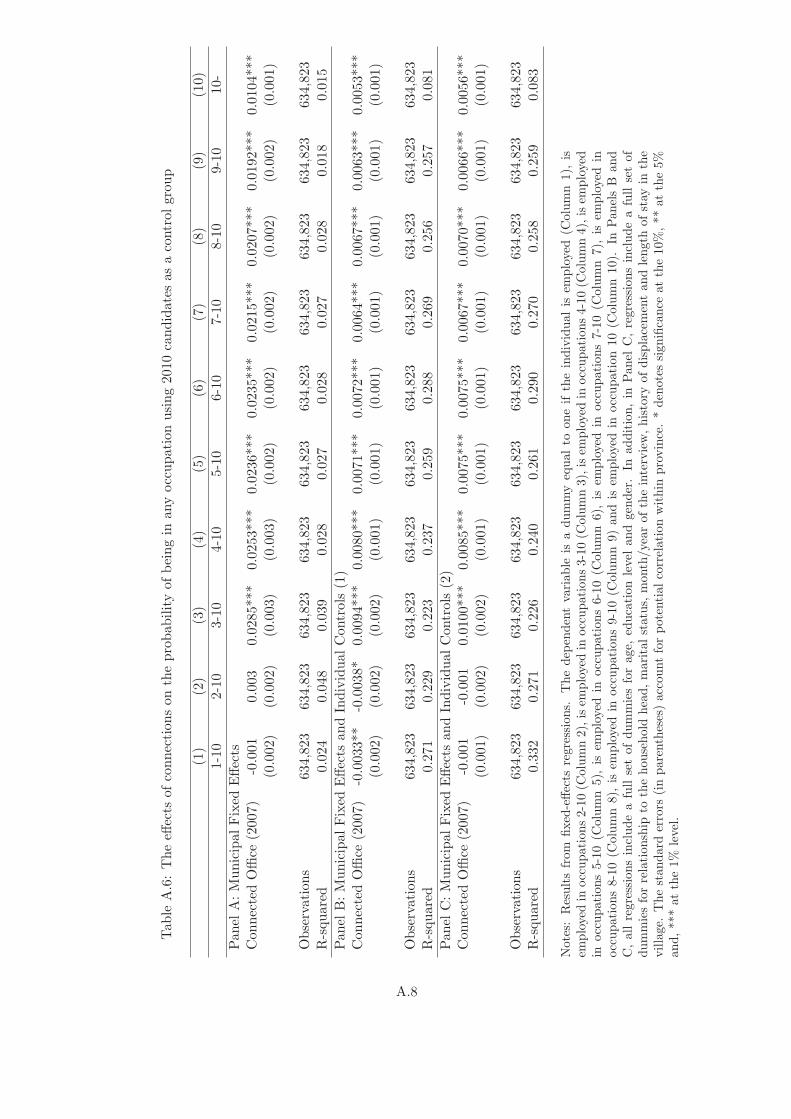
Table
A.6:Theeff
ects
ofconnectionsontheprobabilityof
beingin
anyoccupationusing2010candidatesas
acontrolgroup
(1)
(2)
(3)
(4)
(5)
(6)
(7)
(8)
(9)
(10)
1-10
2-10
3-10
4-10
5-10
6-10
7-10
8-10
9-10
10-
Pan
elA:MunicipalFixed
Effects
ConnectedOffice
(2007)
-0.001
0.003
0.0285***
0.0253***
0.0236***
0.0235***
0.0215***
0.0207***
0.0192***
0.0104***
(0.002)
(0.002)
(0.003)
(0.003)
(0.002)
(0.002)
(0.002)
(0.002)
(0.002)
(0.001)
Observations
634,823
634,823
634,823
634,823
634,823
634,823
634,823
634,823
634,823
634,823
R-squared
0.024
0.048
0.039
0.028
0.027
0.028
0.027
0.028
0.018
0.015
Pan
elB:MunicipalFixed
Effects
andIndividualControls
(1)
ConnectedOffice
(2007)
-0.0033**
-0.0038*
0.0094***
0.0080***
0.0071***
0.0072***
0.0064***
0.0067***
0.0063***
0.0053***
(0.002)
(0.002)
(0.002)
(0.001)
(0.001)
(0.001)
(0.001)
(0.001)
(0.001)
(0.001)
Observations
634,823
634,823
634,823
634,823
634,823
634,823
634,823
634,823
634,823
634,823
R-squared
0.271
0.229
0.223
0.237
0.259
0.288
0.269
0.256
0.257
0.081
Pan
elC:MunicipalFixed
Effects
andIndividualControls
(2)
ConnectedOffice
(2007)
-0.001
-0.001
0.0100***
0.0085***
0.0075***
0.0075***
0.0067***
0.0070***
0.0066***
0.0056***
(0.001)
(0.002)
(0.002)
(0.001)
(0.001)
(0.001)
(0.001)
(0.001)
(0.001)
(0.001)
Observations
634,823
634,823
634,823
634,823
634,823
634,823
634,823
634,823
634,823
634,823
R-squared
0.332
0.271
0.226
0.240
0.261
0.290
0.270
0.258
0.259
0.083
Notes:
Resultsfrom
fixed
-effects
regressions.
Thedep
endentvariable
isadummyequalto
oneiftheindividualis
employed(C
olumn1),
isem
ployedin
occupations2-10(C
olumn2),isem
ployedin
occupations3-10(C
olumn3),isem
ployedin
occupations4-10(C
olumn4),isem
ployed
inoccupations5-10(C
olumn5),
isem
ployedin
occupations6-10(C
olumn6),
isem
ployedin
occupations7-10(C
olumn7),
isem
ployedin
occupations8-10(C
olumn8),
isem
ployedin
occupations9-10(C
olumn9)andis
employedin
occupation10(C
olumn10).
InPanelsB
and
C,allregressionsincludeafullsetofdummiesforage,
educationlevel
andgender.In
addition,in
Panel
C,regressionsincludeafullsetof
dummiesforrelationship
tothehousehold
head,maritalstatus,
month/yearoftheinterview,history
ofdisplacementan
dlength
ofstay
inthe
village.
Thestandard
errors
(inparentheses)accountforpotentialcorrelationwithin
province.*den
otessignificance
atthe10%,**
atthe5%
and,***atthe1%
level.
A.8
Tab
leA.7:Theeff
ects
ofconnectionsontheprobabilityof
beingin
anyoccupationusingunsuccessful2010candidatesas
acontrol
group
(1)
(2)
(3)
(4)
(5)
(6)
(7)
(8)
(9)
(10)
1-10
2-10
3-10
4-10
5-10
6-10
7-10
8-10
9-10
10-
Pan
elA:MunicipalFixed
Effects
ConnectedOffice
(2007)
-0.000
0.004
0.0300***
0.0272***
0.0251***
0.0250***
0.0228***
0.0219***
0.0202***
0.0106***
(0.002)
(0.002)
(0.003)
(0.003)
(0.002)
(0.002)
(0.002)
(0.002)
(0.002)
(0.001)
Observations
575,871
575,871
575,871
575,871
575,871
575,871
575,871
575,871
575,871
575,871
R-squared
0.025
0.047
0.039
0.028
0.027
0.029
0.028
0.028
0.019
0.016
Pan
elB:MunicipalFixed
Effects
andIndividualControls
(1)
ConnectedOffice
(2007)
-0.0030*
-0.003
0.0096***
0.0088***
0.0075***
0.0076***
0.0067***
0.0069***
0.0065***
0.0053***
(0.002)
(0.002)
(0.002)
(0.001)
(0.001)
(0.001)
(0.001)
(0.001)
(0.001)
(0.001)
Observations
575,871
575,871
575,871
575,871
575,871
575,871
575,871
575,871
575,871
575,871
R-squared
0.270
0.228
0.224
0.239
0.261
0.289
0.269
0.256
0.257
0.082
Pan
elC:MunicipalFixed
Effects
andIndividualControls
(2)
ConnectedOffice
(2007)
-0.000
-0.001
0.0101***
0.0092***
0.0078***
0.0079***
0.0070***
0.0072***
0.0067***
0.0055***
(0.002)
(0.002)
(0.002)
(0.001)
(0.001)
(0.001)
(0.001)
(0.001)
(0.001)
(0.001)
Observations
575,871
575,871
575,871
575,871
575,871
575,871
575,871
575,871
575,871
575,871
R-squared
0.331
0.271
0.227
0.242
0.263
0.291
0.271
0.258
0.259
0.084
Notes:
Resultsfrom
fixed
-effects
regressions.
Thedep
endentvariable
isadummyequalto
oneiftheindividualis
employed(C
olumn1),
isem
ployedin
occupations2-10(C
olumn2),isem
ployedin
occupations3-10(C
olumn3),isem
ployedin
occupations4-10(C
olumn4),isem
ployed
inoccupations5-10(C
olumn5),
isem
ployedin
occupations6-10(C
olumn6),
isem
ployedin
occupations7-10(C
olumn7),
isem
ployedin
occupations8-10(C
olumn8),
isem
ployedin
occupations9-10(C
olumn9)andis
employedin
occupation10(C
olumn10).
InPanelsB
and
C,allregressionsincludeafullsetofdummiesforage,
educationlevel
andgender.In
addition,in
Panel
C,regressionsincludeafullsetof
dummiesforrelationship
tothehousehold
head,maritalstatus,
month/yearoftheinterview,history
ofdisplacementan
dlength
ofstay
inthe
village.
Thestandard
errors
(inparentheses)accountforpotentialcorrelationwithin
province.*den
otessignificance
atthe10%,**
atthe5%
and,***atthe1%
level.
A.9

Tab
leA.8:Theeff
ects
ofconnectionsontheprobabilityof
beingin
anyoccupationusingsuccessful2010candidatesas
acontrol
group
(1)
(2)
(3)
(4)
(5)
(6)
(7)
(8)
(9)
(10)
1-10
2-10
3-10
4-10
5-10
6-10
7-10
8-10
9-10
10-
Pan
elA:MunicipalFixed
Effects
ConnectedOffice
(2007)
-0.001
0.002
0.0230***
0.0192***
0.0190***
0.0194***
0.0181***
0.0176***
0.0164***
0.0093***
(0.003)
(0.003)
(0.004)
(0.004)
(0.003)
(0.003)
(0.003)
(0.003)
(0.003)
(0.002)
Observations
454,344
454,344
454,344
454,344
454,344
454,344
454,344
454,344
454,344
454,344
R-squared
0.025
0.048
0.038
0.028
0.028
0.029
0.028
0.029
0.020
0.018
Pan
elB:MunicipalFixed
Effects
andIndividualControls
(1)
ConnectedOffice
(2007)
-0.004
-0.005
0.0078***
0.0053**
0.0057***
0.0062***
0.0058***
0.0061***
0.0058***
0.0052***
(0.003)
(0.003)
(0.003)
(0.002)
(0.002)
(0.002)
(0.002)
(0.002)
(0.002)
(0.001)
Observations
454,344
454,344
454,344
454,344
454,344
454,344
454,344
454,344
454,344
454,344
R-squared
0.271
0.229
0.229
0.243
0.266
0.295
0.275
0.263
0.263
0.086
Pan
elC:MunicipalFixed
Effects
andIndividualControls
(2)
ConnectedOffice
(2007)
-0.002
-0.002
0.0085***
0.0060***
0.0062***
0.0066***
0.0062***
0.0065***
0.0061***
0.0054***
(0.003)
(0.003)
(0.003)
(0.002)
(0.002)
(0.002)
(0.002)
(0.002)
(0.002)
(0.001)
Observations
454,344
454,344
454,344
454,344
454,344
454,344
454,344
454,344
454,344
454,344
R-squared
0.331
0.271
0.232
0.246
0.268
0.297
0.277
0.264
0.264
0.088
Notes:
Resultsfrom
fixed
-effects
regressions.
Thedep
endentvariable
isadummyequalto
oneiftheindividualis
employed(C
olumn1),
isem
ployedin
occupations2-10(C
olumn2),isem
ployedin
occupations3-10(C
olumn3),isem
ployedin
occupations4-10(C
olumn4),isem
ployed
inoccupations5-10(C
olumn5),
isem
ployedin
occupations6-10(C
olumn6),
isem
ployedin
occupations7-10(C
olumn7),
isem
ployedin
occupations8-10(C
olumn8),
isem
ployedin
occupations9-10(C
olumn9)andis
employedin
occupation10(C
olumn10).
InPanelsB
and
C,allregressionsincludeafullsetofdummiesforage,
educationlevel
andgender.In
addition,in
Panel
C,regressionsincludeafullsetof
dummiesforrelationship
tothehousehold
head,maritalstatus,
month/yearoftheinterview,history
ofdisplacementan
dlength
ofstay
inthe
village.
Thestandard
errors
(inparentheses)accountforpotentialcorrelationwithin
province.*den
otessignificance
atthe10%,**
atthe5%
and,***atthe1%
level.
A.10

Tab
leA.9:Theeff
ects
ofconnectionsontheprobabilityof
beingin
anyoccupationusingunsuccessful2007candidatesas
acontrol
group(m
ayors/vice-mayors
only)
(1)
(2)
(3)
(4)
(5)
(6)
(7)
(8)
(9)
(10)
1-10
2-10
3-10
4-10
5-10
6-10
7-10
8-10
9-10
10-
Pan
elA:MunicipalFixed
Effects
ConnectedOffice
(2007)
0.006
0.0131***
0.0278***
0.0262***
0.0240***
0.0246***
0.0228***
0.0225***
0.0204***
0.0124***
(0.003)
(0.003)
(0.004)
(0.003)
(0.003)
(0.003)
(0.003)
(0.003)
(0.002)
(0.002)
Observations
207,314
207,314
207,314
207,314
207,314
207,314
207,314
207,314
207,314
207,314
R-squared
0.027
0.053
0.044
0.034
0.034
0.035
0.034
0.033
0.027
0.023
Pan
elB:MunicipalFixed
Effects
andIndividualControls
(1)
ConnectedOffice
(2007)
0.003
0.0063*
0.0097***
0.0097***
0.0081***
0.0089***
0.0082***
0.0089***
0.0077***
0.0076***
(0.003)
(0.003)
(0.002)
(0.002)
(0.002)
(0.002)
(0.002)
(0.002)
(0.002)
(0.001)
Observations
207,314
207,314
207,314
207,314
207,314
207,314
207,314
207,314
207,314
207,314
R-squared
0.269
0.231
0.239
0.257
0.278
0.306
0.286
0.275
0.276
0.093
Pan
elC:MunicipalFixed
Effects
andIndividualControls
(2)
ConnectedOffice
(2007)
0.004
0.0076**
0.0100***
0.0100***
0.0083***
0.0091***
0.0084***
0.0090***
0.0080***
0.0078***
(0.003)
(0.003)
(0.002)
(0.002)
(0.002)
(0.002)
(0.002)
(0.002)
(0.002)
(0.001)
Observations
207,314
207,314
207,314
207,314
207,314
207,314
207,314
207,314
207,314
207,314
R-squared
0.334
0.276
0.244
0.262
0.282
0.308
0.289
0.277
0.278
0.096
Notes:
Resultsfrom
fixed
-effects
regressions.
Thedep
endentvariable
isadummyequalto
oneiftheindividualis
employed(C
olumn1),
isem
ployedin
occupations2-10(C
olumn2),isem
ployedin
occupations3-10(C
olumn3),isem
ployedin
occupations4-10(C
olumn4),isem
ployed
inoccupations5-10(C
olumn5),
isem
ployedin
occupations6-10(C
olumn6),
isem
ployedin
occupations7-10(C
olumn7),
isem
ployedin
occupations8-10(C
olumn8),
isem
ployedin
occupations9-10(C
olumn9)andis
employedin
occupation10(C
olumn10).
InPanelsB
and
C,allregressionsincludeafullsetofdummiesforage,
educationlevel
andgender.In
addition,in
Panel
C,regressionsincludeafullsetof
dummiesforrelationship
tothehousehold
head,maritalstatus,
month/yearoftheinterview,history
ofdisplacementan
dlength
ofstay
inthe
village.
Thestandard
errors
(inparentheses)accountforpotentialcorrelationwithin
province.*den
otessignificance
atthe10%,**
atthe5%
and,***atthe1%
level.
A.11

Tab
leA.10:Theeff
ects
ofconnectionsontheprobabilityof
beingin
each
occupationusingsuccessful2010candidatesas
acontrol
group
(1)
(2)
(3)
(4)
(5)
(6)
(7)
(8)
(9)
(10)
1-2-
3-4-
5-6-
7-8-
9-10
-
Pan
elA:MunicipalFixed
Effects
ConnectedOffice
(2007)
-0.002
-0.0214***
0.0038**
0.000
-0.000
0.0014***
0.001
0.001
0.0071***
0.0093***
(0.003)
(0.004)
(0.002)
(0.001)
(0.001)
(0.000)
(0.000)
(0.001)
(0.001)
(0.002)
Observations
454,344
454,344
454,344
454,344
454,344
454,344
454,344
454,344
454,344
454,344
R-squared
0.058
0.080
0.033
0.016
0.010
0.006
0.006
0.036
0.013
0.018
Pan
elB:MunicipalFixed
Effects
andIndividualControls
(1)
ConnectedOffice
(2007)
0.001
-0.0123***
0.003
-0.000
-0.001
0.000
-0.000
0.000
0.001
0.0052***
(0.003)
(0.003)
(0.002)
(0.001)
(0.001)
(0.000)
(0.000)
(0.001)
(0.001)
(0.001)
Observations
454,344
454,344
454,344
454,344
454,344
454,344
454,344
454,344
454,344
454,344
R-squared
0.089
0.294
0.044
0.020
0.025
0.024
0.021
0.043
0.202
0.086
Pan
elC:MunicipalFixed
Effects
andIndividualControls
(2)
ConnectedOffice
(2007)
0.001
-0.0109***
0.003
-0.000
-0.000
0.000
-0.000
0.000
0.001
0.0054***
(0.003)
(0.003)
(0.002)
(0.001)
(0.001)
(0.000)
(0.000)
(0.001)
(0.001)
(0.001)
Observations
454,344
454,344
454,344
454,344
454,344
454,344
454,344
454,344
454,344
454,344
R-squared
0.097
0.330
0.045
0.021
0.026
0.026
0.022
0.043
0.202
0.088
Notes:
Resultsfrom
fixed
-effects
regressions.
Thedep
endentvariable
isadummyequalto
oneif
theindividualis
employedin
occupation
1(C
olumn1),
isem
ployedin
occupation2(C
olumn2),
isem
ployedin
occupation3(C
olumn3),
isem
ployed
inoccupation4(C
olumn4),
isem
ployed
inoccupation5(C
olumn5),
isem
ployedin
occupation6(C
olumn6),
isem
ployedin
occupation7(C
olumn7),
isem
ployedin
occupation8(C
olumn8),
isem
ployedin
occupation9(C
olumn9)andis
employedin
occupation10(C
olumn10).
InPanelsB
andC,all
regressionsincludeafullsetofdummiesforage,
educationlevelandgender.In
addition,in
Panel
C,regressionsincludeafullsetofdummies
forrelationship
tothehousehold
head,maritalstatus,
month/yearoftheinterview,history
ofdisplacementandlength
ofstay
inthevillage.
Thestandard
errors
(inparentheses)accountforpotentialcorrelationwithin
province.*den
otessignificance
atthe10%,**at
the5%
and,***
atthe1%
level.
A.12

Tab
leA.11:Theconditionaleff
ects
ofconnectionsontheprobabilityofbeingin
each
occupationusingsuccessful2010candidates
asacontrolgroup
(1)
(2)
(3)
(4)
(5)
(6)
(7)
(8)
(9)
2-10
3-10
4-10
5-10
6-10
7-10
8-10
9-10
10-
Panel
A:MunicipalFixed
Effects
ConnectedOffice
(2007)
0.002
0.0176***
-0.002
0.010
0.0117**
-0.001
0.0102**
0.0151*
0.0239**
(0.004)
(0.004)
(0.007)
(0.006)
(0.005)
(0.005)
(0.005)
(0.008)
(0.010)
Observations
269,482
204,852
85,093
60,409
50,224
43,617
39,822
36,563
30,579
R-squared
0.107
0.475
0.210
0.219
0.312
0.084
0.115
0.286
0.287
Panel
B:MunicipalFixed
Effects
andIndividualControls
(1)
ConnectedOffice
(2007)
-0.004
0.0174***
-0.003
0.009
0.0114**
-0.002
0.0097**
0.0157*
0.0231**
(0.004)
(0.004)
(0.007)
(0.006)
(0.005)
(0.005)
(0.005)
(0.009)
(0.010)
Observations
269,482
204,852
85,093
60,409
50,224
43,617
39,822
36,563
30,579
R-squared
0.152
0.471
0.206
0.215
0.305
0.077
0.109
0.280
0.278
Panel
C:MunicipalFixed
Effects
andIndividualControls
(2)
ConnectedOffice
(2007)
-0.003
0.0176***
-0.002
0.010
0.0117**
-0.001
0.0102**
0.0151*
0.0239**
(0.004)
(0.004)
(0.007)
(0.006)
(0.005)
(0.005)
(0.005)
(0.008)
(0.010)
Observations
269,482
204,852
85,093
60,409
50,224
43,617
39,822
36,563
30,579
R-squared
0.159
0.475
0.210
0.219
0.312
0.084
0.115
0.286
0.287
Notes:
Resultsfrom
fixed
-effects
regressions.
Thedep
endentvariable
isadummyequalto
oneiftheindividualisem
ployedin
occupations2-10
(Column1),isem
ployedin
occupations3-10(C
olumn2),isem
ployedin
occupations4-10(C
olumn3),isem
ployedin
occupations5-10(C
olumn
4),
isem
ployedin
occupations6-10(C
olumn5),
isem
ployed
inoccupations7-10(C
olumn6),
isem
ployedin
occupations8-10(C
olumn7),
isem
ployedin
occupations9-10(C
olumn8)andisem
ployed
inoccupation10(C
olumn9).In
Pan
elsB
andC,allregressionsincludeafullsetof
dummiesforage,
educationlevelandgender.In
addition,in
Panel
C,regressionsincludeafullsetofdummiesforrelationship
tothehousehold
head,maritalstatus,month/yearoftheinterview,history
ofdisplacementan
dlength
ofstay
inthevillage.
Thestandard
errors
(inparentheses)
accountforpotentialcorrelationwithin
province.*denotessignificance
atthe10%,**
atthe5%
and,***atthe1%
level.
A.13

Table A.12: The effects of connections on alternative outcomes(1) (2) (1)
Panel A: Municipal Fixed EffectsConnected Office (2007) 7.0985*** 6.9889*** 0.9773***
(1.248) (1.220) (0.153)
Observations 454,889 454,889 454,889R-squared 0.024 0.024 0.029
Panel B: Municipal Fixed Effects and Individual Controls (1)Connected Office (2007) 1.8226** 1.7197** 0.1967**
(0.816) (0.773) (0.093)
Observations 454,889 454,889 454,889R-squared 0.283 0.285 0.254
Panel C: Municipal Fixed Effects and Individual Controls (2)Connected Office (2007) 2.2738*** 2.1457*** 0.2043**
(0.773) (0.736) (0.093)
Observations 454,889 454,889 454,889R-squared 0.306 0.306 0.255
Notes: Results from fixed-effects regressions. The dependent variable is equal to average wage of in-dividuals employed in the same occupation as the individual (Column 1). The dependent variable isequal to median wage of individuals employed in the same occupation as the individual (Column 2). Thedependent variable is equal to the share of individuals employed in the same occupation as the individualwho are employed in the public sector (Column 3). In Panels B and C, all regressions include a full setof dummies for age, education level and gender. In addition, in Panel C, regressions include a full set ofdummies for relationship to the household head, marital status, month/year of the interview, history ofdisplacement and length of stay in the village. The standard errors (in parentheses) account for potentialcorrelation within province. * denotes significance at the 10%, ** at the 5% and, *** at the 1% level.
A.14

Tab
leA.13:Robustnesschecks:ControllingforNetwork
Size
(1)
(2)
(3)
(4)
(5)
(6)
(7)
(8)
(9)
(10)
1-10
2-10
3-10
4-10
5-10
6-10
7-10
8-10
9-10
10-
Pan
elA:MunicipalFixed
Effects
ConnectedOffice
(2007)
-0.000
0.002
0.0261***
0.0216***
0.0215***
0.0214***
0.0199***
0.0191***
0.0176***
0.0096***
(0.003)
(0.003)
(0.004)
(0.003)
(0.003)
(0.003)
(0.003)
(0.003)
(0.003)
(0.002)
Observations
454,344
454,344
454,344
454,344
454,344
454,344
454,344
454,344
454,344
454,344
R-squared
0.029
0.053
0.042
0.032
0.031
0.032
0.031
0.032
0.023
0.019
Pan
elB:MunicipalFixed
Effects
andIndividualControls
(1)
ConnectedOffice
(2007)
-0.004
-0.005
0.0092***
0.0063***
0.0068***
0.0069***
0.0064***
0.0065***
0.0059***
0.0050***
(0.003)
(0.003)
(0.003)
(0.002)
(0.002)
(0.002)
(0.002)
(0.002)
(0.001)
(0.001)
Observations
454,344
454,344
454,344
454,344
454,344
454,344
454,344
454,344
454,344
454,344
R-squared
0.273
0.232
0.230
0.245
0.267
0.296
0.276
0.264
0.264
0.087
Pan
elC:MunicipalFixed
Effects
andIndividualControls
(2)
ConnectedOffice
(2007)
-0.001
-0.002
0.0097***
0.0067***
0.0070***
0.0071***
0.0067***
0.0068***
0.0062***
0.0052***
(0.003)
(0.003)
(0.003)
(0.002)
(0.002)
(0.002)
(0.002)
(0.002)
(0.001)
(0.001)
Observations
454,344
454,344
454,344
454,344
454,344
454,344
454,344
454,344
454,344
454,344
R-squared
0.332
0.273
0.233
0.247
0.269
0.298
0.278
0.265
0.265
0.089
Notes:
Resultsfrom
fixed
-effects
regressions.
Thedep
endentvariable
isadummyequalto
oneif
theindividualis
employed
(Column
1),
isem
ployedin
occupations2-10(C
olumn2),
isem
ployedin
occupations3-10(C
olumn3),
isem
ployed
inoccupations4-10(C
olumn4),
isem
ployed
inoccupations5-10(C
olumn
5),
isem
ployed
inoccupations6-10(C
olumn
6),
isem
ployed
inoccupations7-10(C
olumn
7),
isem
ployedin
occupations8-10(C
olumn8),
isem
ployedin
occupations9-10(C
olumn9)
andis
employedin
occupation10(C
olumn10).
All
regressionsincludeafullof
setofdummiesforthenumber
ofindividuals
whoshare
theindividual’smiddle
namein
themunicipality
andfor
thenumber
ofindividuals
whoshare
theindividual’smiddle
namein
themunicipality.In
PanelsB
andC,allregressionsincludeafullsetof
dummiesforage,
educationlevelandgender.In
addition,in
Panel
C,regressionsincludeafullsetofdummiesforrelationship
tothehousehold
head,maritalstatus,month/yearoftheinterview,history
ofdisplacementan
dlength
ofstay
inthevillage.
Thestandard
errors
(inparentheses)
accountforpotentialcorrelationwithin
province.*denotessignificance
atthe10%,**
atthe5%
and,***atthe1%
level.
A.15

Tab
leA.14:Robustnesschecks:
Tow
ardsafullysaturatedmodel
(1)
(2)
(3)
(4)
(5)
(6)
(7)
(8)
(9)
(10)
1-10
2-10
3-10
4-10
5-10
6-10
7-10
8-10
9-10
10-
Pan
elA:Interact
allvariableswithgender
ConnectedOffice
(2007)
-0.002
-0.002
0.0085***
0.0059***
0.0062***
0.0066***
0.0062***
0.0065***
0.0061***
0.0054***
(0.003)
(0.003)
(0.003)
(0.002)
(0.002)
(0.002)
(0.002)
(0.002)
(0.002)
(0.001)
Observations
454,344
454,344
454,344
454,344
454,344
454,344
454,344
454,344
454,344
454,344
R-squared
0.351
0.282
0.236
0.250
0.271
0.298
0.278
0.266
0.266
0.089
Pan
elB:Age/Edu/Gender
specificdummies
ConnectedOffice
(2007)
-0.002
-0.002
0.0082***
0.0056***
0.0059***
0.0063***
0.0059***
0.0061***
0.0058***
0.0052***
(0.003)
(0.003)
(0.003)
(0.002)
(0.002)
(0.002)
(0.002)
(0.002)
(0.002)
(0.001)
Observations
454,344
454,344
454,344
454,344
454,344
454,344
454,344
454,344
454,344
454,344
R-squared
0.355
0.287
0.248
0.264
0.287
0.315
0.297
0.286
0.288
0.104
Pan
elC:Age/Edu/Gen
der/Province
specificdummies
ConnectedOffice
(2007)
-0.001
-0.002
0.0084**
0.0053**
0.0056***
0.0059***
0.0052***
0.0054***
0.0049***
0.0043***
(0.003)
(0.004)
(0.003)
(0.002)
(0.002)
(0.002)
(0.002)
(0.002)
(0.002)
(0.001)
Observations
454,344
454,344
454,344
454,344
454,344
454,344
454,344
454,344
454,344
454,344
R-squared
0.461
0.405
0.366
0.379
0.399
0.425
0.408
0.399
0.395
0.263
Pan
elC:Age/Edu/Gen
der/Munispecificdummies
ConnectedOffice
(2007)
-0.003
-0.000
0.0106***
0.0071***
0.0066***
0.0064***
0.0045**
0.0047**
0.0050***
0.0036**
(0.003)
(0.004)
(0.003)
(0.003)
(0.002)
(0.002)
(0.002)
(0.002)
(0.002)
(0.002)
Observations
454,344
454,344
454,344
454,344
454,344
454,344
454,344
454,344
454,344
454,344
R-squared
0.073
0.042
0.008
0.006
0.005
0.004
0.004
0.003
0.003
0.003
Notes:
Resultsfrom
fixed
-effects
regressions.
Thedep
endentvariable
isadummyequalto
oneif
theindividualis
employed
(Column
1),
isem
ployedin
occupations2-10(C
olumn2),
isem
ployedin
occupations3-10(C
olumn3),
isem
ployed
inoccupations4-10(C
olumn4),
isem
ployed
inoccupations5-10(C
olumn
5),
isem
ployed
inoccupations6-10(C
olumn
6),
isem
ployed
inoccupations7-10(C
olumn
7),
isem
ployedin
occupations8-10(C
olumn8),
isem
ployedin
occupations9-10(C
olumn9)
andis
employedin
occupation10(C
olumn10).
All
regressionsincludeafullsetofdummiesforage,
educationlevel,gender,forrelationship
tothehousehold
head,maritalstatus,
month/yearof
theinterview,history
ofdisplacementan
dlength
ofstay
inthevillage.
InPanel
A,allvariablesare
interacted
withthegen
der
dummy.
InPanel
B,regressionsarefullysaturatedforage,
educationan
dgender.In
Pan
elC,theage*education*gender
dummiesare
interacted
withprovince
dummies.
InPan
elD,theage*ed
ucation*gen
der
dummiesare
interacted
withmunicipaldummies.
Thestandard
errors
(inparentheses)account
forpotentialcorrelationwithin
province.*denotessignificance
atthe10%,**
atthe5%
and,***atthe1%
level.
A.16
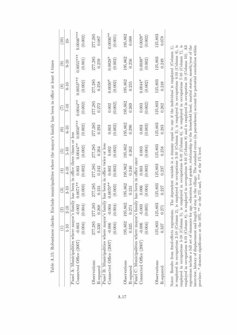
Tab
leA.15:Robustnesschecks:
Excludemunicipalities
wherethemayor’sfamilyhasbeenin
office
atleast
4times
(1)
(2)
(3)
(4)
(5)
(6)
(7)
(8)
(9)
(10)
1-10
2-10
3-10
4-10
5-10
6-10
7-10
8-10
9-10
10-
Pan
elA:Municipalities
wheremayor’s
familyhasbeenin
office
threetimes
orless
ConnectedOffice
(2007)
-0.003
-0.002
0.0071**
0.003
0.0044**
0.0050***
0.0044**
0.0053***
0.0055***
0.0046***
(0.004)
(0.004)
(0.003)
(0.002)
(0.002)
(0.002)
(0.002)
(0.002)
(0.001)
(0.002)
Observations
277,285
277,285
277,285
277,285
277,285
277,285
277,285
277,285
277,285
277,285
R-squared
0.330
0.268
0.231
0.243
0.264
0.293
0.272
0.258
0.259
0.087
Pan
elB:Municipalities
wheremayor’s
familyhasbeenin
office
twiceor
less
ConnectedOffice
(2007)
-0.006
-0.004
0.0070**
0.003
0.002
0.003
0.002
0.0030*
0.0028*
0.0036**
(0.004)
(0.004)
(0.003)
(0.003)
(0.002)
(0.002)
(0.002)
(0.002)
(0.002)
(0.001)
Observations
195,862
195,862
195,862
195,862
195,862
195,862
195,862
195,862
195,862
195,862
R-squared
0.335
0.274
0.231
0.240
0.262
0.290
0.269
0.255
0.256
0.088
Pan
elC:Municipalities
wheremayor’s
familyhasbeenin
office
once
ConnectedOffice
(2007)
-0.006
-0.003
0.006
0.003
0.003
0.003
0.003
0.0044*
0.0038*
0.0028*
(0.004)
(0.005)
(0.004)
(0.003)
(0.004)
(0.003)
(0.002)
(0.002)
(0.002)
(0.002)
Observations
125,803
125,803
125,803
125,803
125,803
125,803
125,803
125,803
125,803
125,803
R-squared
0.337
0.271
0.227
0.237
0.258
0.283
0.262
0.248
0.249
0.078
Notes:
Resultsfrom
fixed
-effects
regressions.
Thedep
endentvariable
isadummyequalto
oneif
theindividualis
employed
(Column
1),
isem
ployedin
occupations2-10(C
olumn2),
isem
ployedin
occupations3-10(C
olumn3),
isem
ployed
inoccupations4-10(C
olumn4),
isem
ployed
inoccupations5-10(C
olumn
5),
isem
ployed
inoccupations6-10(C
olumn
6),
isem
ployed
inoccupations7-10(C
olumn
7),
isem
ployedin
occupations8-10(C
olumn8),
isem
ployedin
occupations9-10(C
olumn9)
andis
employedin
occupation10(C
olumn10).
All
regressionsincludeafullsetofdummiesforage,
educationlevelgen
der,relationship
tothehousehold
head,maritalstatus,
month/yearofthe
interview,history
ofdisplacementan
dlength
ofstay
inthevillage.
Thestandard
errors
(inparentheses)accountforpotentialcorrelationwithin
province.*denotessignificance
atthe10%,**
atthe5%
and,***atthe1%
level.
A.17

Tab
leA.16:Themarginaleff
ects
ofconnectionsto
each
typeofelectedofficialontheprobabilityof
beingin
anyoccupation-all
possible
interactions
(1)
(2)
(3)
(4)
(5)
(6)
(7)
(8)
(9)
(10)
1-10
2-10
3-10
4-10
5-10
6-10
7-10
8-10
9-10
10-
Pan
elA:MunicipalFixed
Effects
andIndividualControls
(2)
A:Mayor
(2007)
0.003
-0.001
0.0154***
0.0141***
0.0132***
0.0125***
0.0108***
0.0109***
0.0093***
0.0079***
(0.003)
(0.004)
(0.002)
(0.002)
(0.002)
(0.002)
(0.002)
(0.002)
(0.002)
(0.002)
B:Vice-Mayor
(2007)
0.001
0.004
0.0100***
0.0085***
0.0063**
0.0070***
0.0061***
0.0066***
0.0060**
0.0057***
(0.004)
(0.004)
(0.003)
(0.003)
(0.002)
(0.002)
(0.002)
(0.002)
(0.003)
(0.002)
C:Councilor(2007)
0.000
-0.002
0.0084***
0.0062***
0.0055***
0.0056***
0.0051***
0.0053***
0.0045***
0.0042***
(0.003)
(0.003)
(0.002)
(0.002)
(0.002)
(0.001)
(0.001)
(0.001)
(0.001)
(0.001)
TestH0:A
=B
0.034
0.856
1.854
2.248
5.232
3.482
2.564
1.977
1.096
0.776
Ha:
A�=
B[p-value]
[0.854]
[0.355]
[0.173]
[0.134]
[0.022]
[0.062]
[0.109]
[0.160]
[0.295]
[0.378]
TestH0:A
=C
0.363
0.022
4.518
6.224
9.054
8.333
5.106
5.406
3.966
3.622
Ha:
A�=
C[p-value]
[0.547]
[0.882]
[0.034]
[0.013]
[0.003]
[0.004]
[0.024]
[0.020]
[0.046]
[0.057]
TestH0:B
=C
0.068
1.292
0.157
0.651
0.083
0.350
0.203
0.328
0.259
0.414
Ha:
B�=
C[p-value]
[0.794]
[0.256]
[0.692]
[0.420]
[0.773]
[0.554]
[0.652]
[0.567]
[0.611]
[0.520]
Observations
454,344
454,344
454,344
454,344
454,344
454,344
454,344
454,344
454,344
454,344
Notes:
Meanmarginaleff
ects
from
fixed-effects
regressions.
Theregressionsincludeallpossible
interactionsofthethreedummies(A
,B
and
C).
Thedep
endentvariable
isadummyequalto
oneif
theindividualis
employed
(Column
1),
isem
ployed
inoccupations2-10(C
olumn
2),
isem
ployedin
occupations3-10(C
olumn3),
isem
ployed
inoccupations4-10(C
olumn4),
isem
ployedin
occupations5-10(C
olumn5),
isem
ployedin
occupations6-10(C
olumn6),isem
ployedin
occupations7-10(C
olumn7),isem
ployedin
occupations8-10(C
olumn8),isem
ployed
inoccupations9-10(C
olumn9)andisem
ployedin
occupation10
(Column10).
Allregressionsincludeafullsetofdummiesforage,
education
level,gen
der,relationship
tothehousehold
head,maritalstatus,month/yearoftheinterview,history
ofdisplacementan
dlength
ofstay
inthe
village.
Thestandard
errors
(inparentheses)accountforpotentialcorrelationwithin
province.*den
otessignificance
atthe10%,**
atthe5%
and,***atthe1%
level.
A.18

Tab
leA.17:Municipalheterogen
eity:Municipalcouncil
(1)
(2)
(3)
(4)
(5)
(6)
(7)
(8)
(9)
(10)
1-10
2-10
3-10
4-10
5-10
6-10
7-10
8-10
9-10
10-
Pan
elA:MunicipalFixed
Effects
andIndividualControls
(2)
Mayor
(2007)
-0.000
-0.003
0.0125***
0.0125***
0.0117***
0.0113***
0.0102***
0.0103***
0.0088***
0.0073***
(0.003)
(0.003)
(0.002)
(0.002)
(0.002)
(0.002)
(0.002)
(0.002)
(0.002)
(0.001)
Vice-Mayor
(2007)
-0.002
0.003
0.0116***
0.0091***
0.0080***
0.0090***
0.0080***
0.0087***
0.0078***
0.0069***
(0.003)
(0.004)
(0.003)
(0.003)
(0.003)
(0.002)
(0.002)
(0.002)
(0.002)
(0.002)
Councilor(2007)
0.001
-0.002
0.0091***
0.0069***
0.0057***
0.0056***
0.0049***
0.0050***
0.0040***
0.0040***
(0.003)
(0.003)
(0.002)
(0.002)
(0.002)
(0.001)
(0.001)
(0.001)
(0.001)
(0.001)
Int.
Mayor
(2007)
-0.009
-0.014
-0.013
-0.0158*
-0.0139*
-0.012
-0.0130*
-0.0140*
-0.0122*
-0.0115*
(0.008)
(0.014)
(0.009)
(0.008)
(0.008)
(0.008)
(0.008)
(0.008)
(0.006)
(0.006)
Int.
Vice-Mayor
(2007)
-0.0208*
-0.013
-0.0162*
-0.013
-0.0188**
-0.0138*
-0.011
-0.009
-0.007
-0.005
(0.012)
(0.015)
(0.008)
(0.009)
(0.008)
(0.007)
(0.007)
(0.007)
(0.006)
(0.005)
Int.
Councilor(2007)
0.004
0.000
-0.001
-0.003
-0.006
-0.006
-0.005
-0.003
0.000
-0.005
(0.006)
(0.009)
(0.008)
(0.007)
(0.007)
(0.007)
(0.007)
(0.006)
(0.005)
(0.004)
Observations
451,715
451,715
451,715
451,715
451,715
451,715
451,715
451,715
451,715
451,715
R-squared
0.330
0.271
0.232
0.246
0.268
0.297
0.277
0.265
0.264
0.088
Notes:
Resultsfrom
fixed
-effects
regressions.
Thedep
endentvariable
isadummyequalto
oneif
theindividualis
employed
(Column
1),
isem
ployedin
occupations2-10(C
olumn2),
isem
ployedin
occupations3-10(C
olumn3),
isem
ployed
inoccupations4-10(C
olumn4),
isem
ployed
inoccupations5-10(C
olumn
5),
isem
ployed
inoccupations6-10(C
olumn
6),
isem
ployed
inoccupations7-10(C
olumn
7),
isem
ployedin
occupations8-10(C
olumn8),
isem
ployedin
occupations9-10(C
olumn9)
andis
employedin
occupation10(C
olumn10).
All
regressionsincludeafullsetofdummiesforage,
educationlevel,gender,relationship
tothehousehold
head,maritalstatus,
month/yearofthe
interview,history
ofdisplacementan
dlength
ofstay
inthevillage.
Thestandard
errors
(inparentheses)accountforpotentialcorrelationwithin
province.*denotessignificance
atthe10%,**
atthe5%
and,***atthe1%
level.
A.19

Tab
leA.18:Municipalheterogen
eity:W
ithin-FamilyFeu
d
(1)
(2)
(3)
(4)
(5)
(6)
(7)
(8)
(9)
(10)
1-10
2-10
3-10
4-10
5-10
6-10
7-10
8-10
9-10
10-
Pan
elA:MunicipalFixed
Effects
ConnectedOffice
(2007)
0.000
0.003
0.0254***
0.0213***
0.0214***
0.0215***
0.0200***
0.0196***
0.0180***
0.0104***
(0.003)
(0.004)
(0.005)
(0.004)
(0.004)
(0.004)
(0.004)
(0.003)
(0.003)
(0.002)
Interaction
-0.005
-0.009
-0.0168*
-0.0148**
-0.0166**
-0.0144**
-0.0129*
-0.0139**
-0.0109*
-0.0077*
(0.007)
(0.008)
(0.008)
(0.007)
(0.007)
(0.007)
(0.006)
(0.006)
(0.006)
(0.004)
Observations
454,344
454,344
454,344
454,344
454,344
454,344
454,344
454,344
454,344
454,344
R-squared
0.025
0.048
0.038
0.028
0.028
0.029
0.028
0.029
0.020
0.018
Pan
elB:MunicipalFixed
Effects
andIndividualControls
(1)
ConnectedOffice
(2007)
-0.003
-0.004
0.0092***
0.0065***
0.0072***
0.0074***
0.0068***
0.0073***
0.0066***
0.0060***
(0.003)
(0.003)
(0.003)
(0.002)
(0.002)
(0.002)
(0.002)
(0.002)
(0.002)
(0.001)
Interaction
-0.003
-0.005
-0.010
-0.0084**
-0.0103**
-0.0081**
-0.0071*
-0.0085**
-0.0059*
-0.0056*
(0.007)
(0.008)
(0.006)
(0.004)
(0.004)
(0.004)
(0.004)
(0.003)
(0.003)
(0.003)
Observations
454,344
454,344
454,344
454,344
454,344
454,344
454,344
454,344
454,344
454,344
R-squared
0.271
0.229
0.229
0.243
0.266
0.295
0.275
0.263
0.263
0.086
Pan
elC:MunicipalFixed
Effects
andIndividualControls
(2)
ConnectedOffice
(2007)
-0.001
-0.002
0.0096***
0.0068***
0.0074***
0.0076***
0.0070***
0.0075***
0.0068***
0.0061***
(0.003)
(0.003)
(0.003)
(0.002)
(0.002)
(0.002)
(0.002)
(0.002)
(0.002)
(0.001)
Interaction
-0.004
-0.005
-0.0102*
-0.0083**
-0.0101**
-0.0079**
-0.0069*
-0.0083**
-0.0057*
-0.0055*
(0.007)
(0.007)
(0.006)
(0.004)
(0.004)
(0.004)
(0.004)
(0.003)
(0.003)
(0.003)
Observations
454,344
454,344
454,344
454,344
454,344
454,344
454,344
454,344
454,344
454,344
R-squared
0.331
0.271
0.231
0.246
0.268
0.297
0.277
0.264
0.264
0.088
Notes:
Resultsfrom
fixed
-effects
regressions.
Theinteractionvariable
isadummyequalto
oneiftheindividualis
connectedto
apolitician
inoffice
inamunicipality
wheremem
bersofthesamefamilycompeted
against
each
other
inmayoralelections.
Thedep
endentvariable
isa
dummyequalto
oneiftheindividualis
employed(C
olumn1),
isem
ployedin
occupations2-10(C
olumn2),
isem
ployedin
occupations3-10
(Column3),isem
ployedin
occupations4-10(C
olumn4),isem
ployedin
occupations5-10(C
olumn5),isem
ployedin
occupations6-10(C
olumn
6),
isem
ployedin
occupations7-10(C
olumn7),
isem
ployedin
occupations8-10(C
olumn8),
isem
ployedin
occupations9-10(C
olumn9)and
isem
ployedin
occupation10(C
olumn10).
InPanelsB
andC,allregressionsincludeafullsetofdummiesforage,
educationlevelandgen
der.
Inaddition,in
Panel
C,regressionsincludeafullsetofdummiesforrelationship
tothehousehold
head,maritalstatus,
month/yearofthe
interview,history
ofdisplacementan
dlength
ofstay
inthevillage.
Thestandard
errors
(inparentheses)accountforpotentialcorrelationwithin
province.*denotessignificance
atthe10%,**
atthe5%
and,***atthe1%
level.
A.20

Tab
leA.19:Robustnesschecks:
Municipalclustering
(1)
(2)
(3)
(4)
(5)
(6)
(7)
(8)
(9)
(10)
1-10
2-10
3-10
4-10
5-10
6-10
7-10
8-10
9-10
10-
Pan
elA:MunicipalFixed
Effects
ConnectedOffice
(2007)
-0.001
0.002
0.0230***
0.0192***
0.0190***
0.0194***
0.0181***
0.0176***
0.0164***
0.0093***
(0.003)
(0.003)
(0.003)
(0.003)
(0.003)
(0.003)
(0.003)
(0.002)
(0.002)
(0.001)
Observations
454,344
454,344
454,344
454,344
454,344
454,344
454,344
454,344
454,344
454,344
R-squared
0.025
0.048
0.038
0.028
0.028
0.029
0.028
0.029
0.020
0.018
Pan
elB:MunicipalFixed
Effects
andIndividualControls
(1)
ConnectedOffice
(2007)
-0.004
-0.005
0.0078***
0.0053***
0.0057***
0.0062***
0.0058***
0.0061***
0.0058***
0.0052***
(0.003)
(0.003)
(0.002)
(0.002)
(0.002)
(0.001)
(0.001)
(0.001)
(0.001)
(0.001)
Observations
454,344
454,344
454,344
454,344
454,344
454,344
454,344
454,344
454,344
454,344
R-squared
0.271
0.229
0.229
0.243
0.266
0.295
0.275
0.263
0.263
0.086
Pan
elC:MunicipalFixed
Effects
andIndividualControls
(2)
ConnectedOffice
(2007)
-0.002
-0.002
0.0085***
0.0060***
0.0062***
0.0066***
0.0062***
0.0065***
0.0061***
0.0054***
(0.003)
(0.003)
(0.002)
(0.002)
(0.002)
(0.001)
(0.001)
(0.001)
(0.001)
(0.001)
Observations
454,344
454,344
454,344
454,344
454,344
454,344
454,344
454,344
454,344
454,344
R-squared
0.331
0.271
0.232
0.246
0.268
0.297
0.277
0.264
0.264
0.088
Notes:
Resultsfrom
fixed
-effects
regressions.
Thedep
endentvariable
isadummyequalto
oneiftheindividualis
employed(C
olumn1),
isem
ployedin
occupations2-10(C
olumn2),isem
ployedin
occupations3-10(C
olumn3),isem
ployedin
occupations4-10(C
olumn4),isem
ployed
inoccupations5-10(C
olumn5),
isem
ployedin
occupations6-10(C
olumn6),
isem
ployedin
occupations7-10(C
olumn7),
isem
ployedin
occupations8-10(C
olumn8),
isem
ployedin
occupations9-10(C
olumn9)andis
employedin
occupation10(C
olumn10).
InPanelsB
and
C,allregressionsincludeafullsetofdummiesforage,
educationlevel
andgender.In
addition,in
Panel
C,regressionsincludeafullsetof
dummiesforrelationship
tothehousehold
head,maritalstatus,
month/yearoftheinterview,history
ofdisplacementan
dlength
ofstay
inthe
village.
Thestandard
errors
(inparentheses)accountforpotentialcorrelationwithin
municipality.*den
otessignificance
atthe10%,**atthe
5%
and,***atthe1%
level.
A.21

Table
A.20:Robustnesschecks:
Two-way
clustering
(1)
(2)
(3)
(4)
(5)
(6)
(7)
(8)
(9)
(10)
1-10
2-10
3-10
4-10
5-10
6-10
7-10
8-10
9-10
10-
Pan
elA:MunicipalFixed
Effects
ConnectedOffice
(2007)
-0.001
0.002
0.0230***
0.0192***
0.0190***
0.0194***
0.0181***
0.0176***
0.0164***
0.0093***
(0.003)
(0.003)
(0.004)
(0.004)
(0.003)
(0.003)
(0.003)
(0.003)
(0.003)
(0.002)
Observations
454,344
454,344
454,344
454,344
454,344
454,344
454,344
454,344
454,344
454,344
R-squared
0.025
0.048
0.038
0.028
0.028
0.029
0.028
0.029
0.020
0.018
Pan
elB:MunicipalFixed
Effects
andIndividualControls
(1)
ConnectedOffice
(2007)
-0.004
-0.005
0.0078***
0.0053**
0.0057***
0.0062***
0.0058***
0.0061***
0.0058***
0.0052***
(0.003)
(0.003)
(0.003)
(0.003)
(0.002)
(0.002)
(0.002)
(0.002)
(0.002)
(0.001)
Observations
454,344
454,344
454,344
454,344
454,344
454,344
454,344
454,344
454,344
454,344
R-squared
0.271
0.229
0.229
0.243
0.266
0.295
0.275
0.263
0.263
0.086
Pan
elC:MunicipalFixed
Effects
andIndividualControls
(2)
ConnectedOffice
(2007)
-0.002
-0.002
0.0085***
0.0060**
0.0062***
0.0066***
0.0062***
0.0065***
0.0061***
0.0054***
(0.003)
(0.004)
(0.003)
(0.003)
(0.002)
(0.002)
(0.002)
(0.002)
(0.002)
(0.001)
Observations
454,344
454,344
454,344
454,344
454,344
454,344
454,344
454,344
454,344
454,344
R-squared
0.331
0.271
0.232
0.246
0.268
0.297
0.277
0.264
0.264
0.088
Notes:
Resultsfrom
fixed
-effects
regressions.
Thedep
endentvariable
isadummyequalto
oneiftheindividualis
employed(C
olumn1),
isem
ployedin
occupations2-10(C
olumn2),isem
ployedin
occupations3-10(C
olumn3),isem
ployedin
occupations4-10(C
olumn4),isem
ployed
inoccupations5-10(C
olumn5),
isem
ployedin
occupations6-10(C
olumn6),
isem
ployedin
occupations7-10(C
olumn7),
isem
ployedin
occupations8-10(C
olumn8),
isem
ployedin
occupations9-10(C
olumn9)andis
employedin
occupation10(C
olumn10).
InPanelsB
andC,
allregressionsincludeafullsetofdummiesforage,
educationlevelandgender.In
addition,in
Panel
C,regressionsincludeafullsetofdummies
forrelationship
tothehousehold
head,maritalstatus,
month/yearoftheinterview,history
ofdisplacementandlength
ofstay
inthevillage.
Thestandard
errors
(inparentheses)accountforpotentialcorrelationwithin
month/yearoftheinterview
andprovince.*den
otessignificance
atthe10%,**
atthe5%
and,***atthe1%
level.
A.22
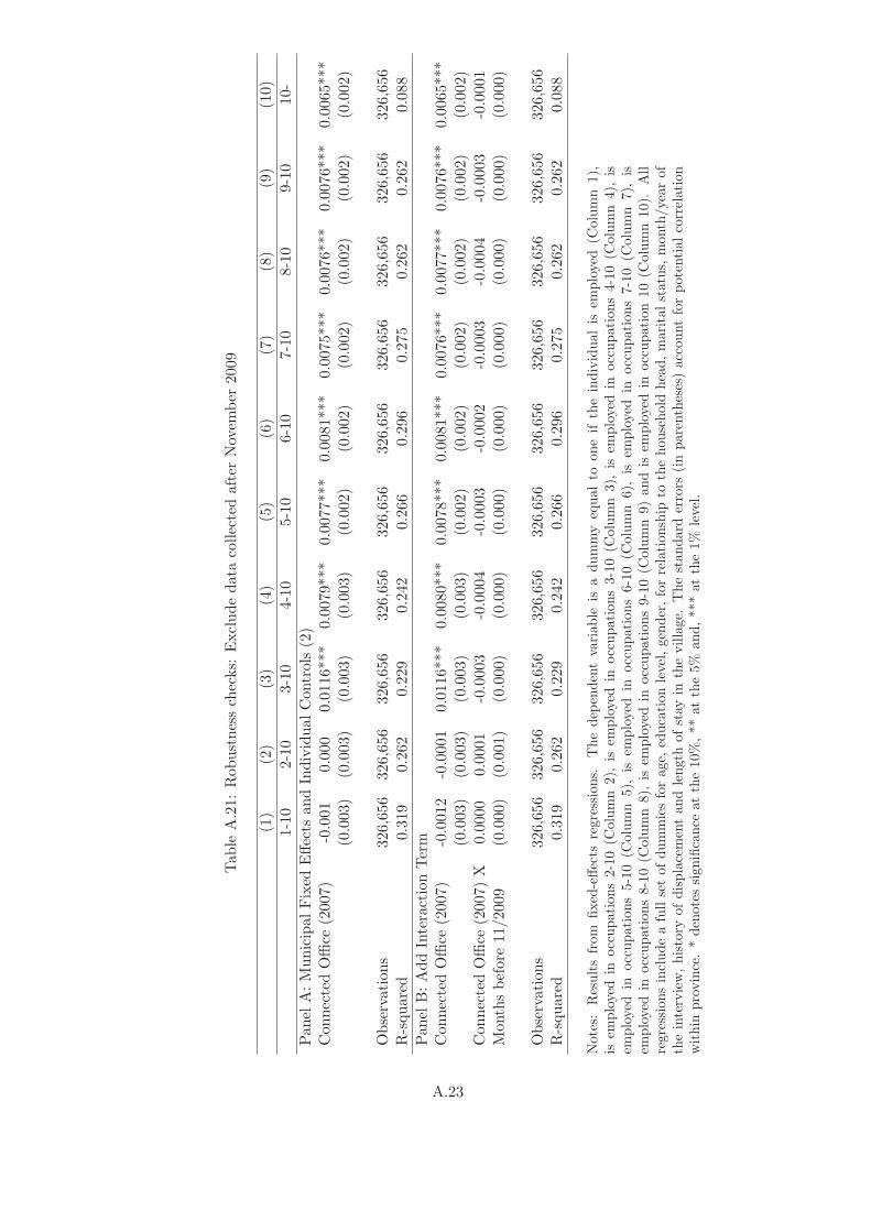
Tab
leA.21:Robustnesschecks:
Excludedata
collectedafter
Novem
ber
2009
(1)
(2)
(3)
(4)
(5)
(6)
(7)
(8)
(9)
(10)
1-10
2-10
3-10
4-10
5-10
6-10
7-10
8-10
9-10
10-
Pan
elA:MunicipalFixed
Effects
andIndividualControls
(2)
ConnectedOffice
(2007)
-0.001
0.000
0.0116***
0.0079***
0.0077***
0.0081***
0.0075***
0.0076***
0.0076***
0.0065***
(0.003)
(0.003)
(0.003)
(0.003)
(0.002)
(0.002)
(0.002)
(0.002)
(0.002)
(0.002)
Observations
326,656
326,656
326,656
326,656
326,656
326,656
326,656
326,656
326,656
326,656
R-squared
0.319
0.262
0.229
0.242
0.266
0.296
0.275
0.262
0.262
0.088
Pan
elB:AddInteractionTerm
ConnectedOffice
(2007)
-0.0012
-0.0001
0.0116***
0.0080***
0.0078***
0.0081***
0.0076***
0.0077***
0.0076***
0.0065***
(0.003)
(0.003)
(0.003)
(0.003)
(0.002)
(0.002)
(0.002)
(0.002)
(0.002)
(0.002)
ConnectedOffice
(2007)X
0.0000
0.0001
-0.0003
-0.0004
-0.0003
-0.0002
-0.0003
-0.0004
-0.0003
-0.0001
Monthsbefore
11/2009
(0.000)
(0.001)
(0.000)
(0.000)
(0.000)
(0.000)
(0.000)
(0.000)
(0.000)
(0.000)
Observations
326,656
326,656
326,656
326,656
326,656
326,656
326,656
326,656
326,656
326,656
R-squared
0.319
0.262
0.229
0.242
0.266
0.296
0.275
0.262
0.262
0.088
Notes:
Resultsfrom
fixed
-effects
regressions.
Thedep
endentvariable
isadummyequalto
oneif
theindividualis
employed
(Column
1),
isem
ployedin
occupations2-10(C
olumn2),
isem
ployedin
occupations3-10(C
olumn3),
isem
ployed
inoccupations4-10(C
olumn4),
isem
ployed
inoccupations5-10(C
olumn
5),
isem
ployed
inoccupations6-10(C
olumn
6),
isem
ployed
inoccupations7-10(C
olumn
7),
isem
ployedin
occupations8-10(C
olumn8),
isem
ployedin
occupations9-10(C
olumn9)
andis
employedin
occupation10(C
olumn10).
All
regressionsincludeafullsetofdummiesforage,
educationlevel,gender,forrelationship
tothehousehold
head,maritalstatus,
month/yearof
theinterview,history
ofdisplacementandlength
ofstay
inthevillage.
Thestandard
errors
(inparentheses)accountforpotentialcorrelation
within
province.*denotessignificance
atthe10%,**
atthe5%
and,***atthe1%
level.
A.23

Table
A.22:Robustnesschecks:
Alternative
fixed
effects
(1)
(2)
(3)
(4)
(5)
(6)
(7)
(8)
(9)
(10)
1-10
2-10
3-10
4-10
5-10
6-10
7-10
8-10
9-10
10-
Pan
elA:VillageFixed
Effects
andIndividualControls
ConnectedOffice
(2007)
-0.002
-0.002
0.0068***
0.0044*
0.0056***
0.0058***
0.0050***
0.0051***
0.0055***
0.0053***
(0.003)
(0.003)
(0.002)
(0.002)
(0.002)
(0.002)
(0.002)
(0.002)
(0.002)
(0.001)
Observations
454,344
454,344
454,344
454,344
454,344
454,344
454,344
454,344
454,344
454,344
R-squared
0.354
0.308
0.260
0.266
0.285
0.313
0.294
0.282
0.280
0.112
Pan
elB:Enumerator*MunicipalFixed
Effects
andIndividualControls
ConnectedOffice
(2007)
-0.0046*
-0.003
0.0068***
0.0040*
0.0051***
0.0052***
0.0049***
0.0052***
0.0053***
0.0054***
(0.003)
(0.003)
(0.003)
(0.002)
(0.002)
(0.002)
(0.002)
(0.002)
(0.002)
(0.001)
Observations
454,344
454,344
454,344
454,344
454,344
454,344
454,344
454,344
454,344
454,344
R-squared
0.376
0.326
0.284
0.296
0.314
0.342
0.325
0.314
0.309
0.152
Pan
elC:MunicipalFixed
Effects
andIndividualControls
-PROBIT
ConnectedOffice
(2007)
-0.002
-0.003
0.0091***
0.0053***
0.0049***
0.0045***
0.0039***
0.0039***
0.0029***
0.0021***
(0.004)
(0.004)
(0.003)
(0.002)
(0.002)
(0.001)
(0.001)
(0.001)
(0.001)
(0.000)
Observations
454,320
454,307
454,261
454,215
454,200
454,203
454,203
454,203
453,822
451,748
Notes:
Resultsfrom
fixed
-effects
regressions.
InPan
elC,marginaleff
ects
computedatthemeanare
reported.Thedep
endentvariable
isa
dummyequalto
oneiftheindividualis
employed(C
olumn1),
isem
ployedin
occupations2-10(C
olumn2),
isem
ployedin
occupations3-10
(Column3),isem
ployedin
occupations4-10(C
olumn4),isem
ployedin
occupations5-10(C
olumn5),isem
ployedin
occupations6-10(C
olumn
6),
isem
ployedin
occupations7-10(C
olumn7),
isem
ployedin
occupations8-10(C
olumn8),
isem
ployedin
occupations9-10(C
olumn9)and
isem
ployedin
occupation10(C
olumn10).
Allregressionsincludeafullsetofdummiesforage,
educationlevel,gen
der,relationship
tothe
household
head,maritalstatus,
month/yearoftheinterview,history
ofdisplacementan
dlength
ofstay
inthevillage.
Thestandard
errors
(in
parentheses)accountforpotentialcorrelationwithin
province.*denotessignificance
atthe10%,**atthe5%
and,***atthe1%
level.
A.24

Tab
leA.23:Robustnesschecks:
ControlforMeasuresof
NameComplexity
(1)
(2)
(3)
(4)
(5)
(6)
(7)
(8)
(9)
(10)
1-10
2-10
3-10
4-10
5-10
6-10
7-10
8-10
9-10
10-
Pan
elA:MunicipalFixed
Effects
ConnectedOffice
(2007)
-0.001
0.001
0.0227***
0.0189***
0.0186***
0.0191***
0.0177***
0.0172***
0.0162***
0.0092***
(0.003)
(0.003)
(0.004)
(0.003)
(0.003)
(0.003)
(0.003)
(0.003)
(0.003)
(0.002)
Observations
452,949
452,949
452,949
452,949
452,949
452,949
452,949
452,949
452,949
452,949
R-squared
0.025
0.048
0.040
0.030
0.029
0.031
0.030
0.030
0.021
0.018
Pan
elB:MunicipalFixed
Effects
andIndividualControls
(1)
ConnectedOffice
(2007)
-0.004
-0.005
0.0077***
0.0052**
0.0055***
0.0061***
0.0056***
0.0059***
0.0057***
0.0051***
(0.003)
(0.003)
(0.003)
(0.002)
(0.002)
(0.002)
(0.002)
(0.002)
(0.001)
(0.001)
Observations
452,949
452,949
452,949
452,949
452,949
452,949
452,949
452,949
452,949
452,949
R-squared
0.271
0.230
0.229
0.244
0.266
0.295
0.275
0.263
0.263
0.086
Pan
elC:MunicipalFixed
Effects
andIndividualControls
(2)
ConnectedOffice
(2007)
-0.002
-0.003
0.0081***
0.0056***
0.0057***
0.0063***
0.0059***
0.0062***
0.0059***
0.0053***
(0.003)
(0.003)
(0.003)
(0.002)
(0.002)
(0.002)
(0.002)
(0.002)
(0.001)
(0.001)
Observations
452,949
452,949
452,949
452,949
452,949
452,949
452,949
452,949
452,949
452,949
R-squared
0.331
0.271
0.232
0.246
0.268
0.297
0.277
0.264
0.264
0.088
Notes:
Resultsfrom
fixed
-effects
regressions.
Thedep
endentvariable
isadummyequalto
oneiftheindividualis
employed(C
olumn1),
isem
ployedin
occupations2-10(C
olumn2),isem
ployedin
occupations3-10(C
olumn3),isem
ployedin
occupations4-10(C
olumn4),isem
ployed
inoccupations5-10(C
olumn5),
isem
ployedin
occupations6-10(C
olumn6),
isem
ployedin
occupations7-10(C
olumn7),
isem
ployedin
occupations8-10(C
olumn8),
isem
ployedin
occupations9-10(C
olumn9)andis
employedin
occupation10(C
olumn10).
Allregressions
includeafullsetofdummiesformiddle
namelength,last
namelength,middle
name’sfirstletter,last
name’sfirstletter
andwhether
themiddle
orlast
nameisautochthonousorof
Chineseorigin.In
PanelsB
andC,allregressionsincludeafullsetofdummiesforage,
educationleveland
gender.In
addition,in
Panel
C,regressionsincludeafullsetofdummiesforrelationship
tothehousehold
head,maritalstatus,
month/yearof
theinterview,history
ofdisplacementandlength
ofstay
inthevillage.
Thestandard
errors
(inparentheses)accountforpotentialcorrelation
within
province.*denotessignificance
atthe10%,**
atthe5%
and,***atthe1%
level.
A.25

Table
A.24:Robustnesschecks:
Excludeindividuals
witheither
Autochthonousor
ChineseFam
ilyNames
(1)
(2)
(3)
(4)
(5)
(6)
(7)
(8)
(9)
(10)
1-10
2-10
3-10
4-10
5-10
6-10
7-10
8-10
9-10
10-
Pan
elA:MunicipalFixed
Effects
ConnectedOffice
(2007)
-0.001
0.001
0.0222***
0.0188***
0.0184***
0.0189***
0.0175***
0.0172***
0.0160***
0.0087***
(0.003)
(0.003)
(0.004)
(0.003)
(0.003)
(0.003)
(0.003)
(0.003)
(0.003)
(0.002)
Observations
440,376
440,376
440,376
440,376
440,376
440,376
440,376
440,376
440,376
440,376
R-squared
0.025
0.048
0.038
0.027
0.027
0.028
0.028
0.028
0.019
0.017
Pan
elB:MunicipalFixed
Effects
andIndividualControls
(1)
ConnectedOffice
(2007)
-0.004
-0.005
0.0074**
0.0053**
0.0055***
0.0061***
0.0056***
0.0061***
0.0057***
0.0047***
(0.003)
(0.003)
(0.003)
(0.002)
(0.002)
(0.002)
(0.002)
(0.002)
(0.001)
(0.001)
Observations
440,376
440,376
440,376
440,376
440,376
440,376
440,376
440,376
440,376
440,376
R-squared
0.272
0.230
0.227
0.241
0.264
0.294
0.274
0.261
0.262
0.085
Pan
elC:MunicipalFixed
Effects
andIndividualControls
(2)
ConnectedOffice
(2007)
-0.002
-0.003
0.0077***
0.0057**
0.0057***
0.0063***
0.0058***
0.0063***
0.0059***
0.0048***
(0.003)
(0.003)
(0.003)
(0.002)
(0.002)
(0.002)
(0.002)
(0.002)
(0.001)
(0.001)
Observations
440,376
440,376
440,376
440,376
440,376
440,376
440,376
440,376
440,376
440,376
R-squared
0.332
0.272
0.230
0.244
0.266
0.295
0.275
0.263
0.263
0.087
Notes:
Resultsfrom
fixed
-effects
regressions.
Thesample
excludes
individualswitheither
anautochthonousmiddle
orlast
nameor
amiddle
or
last
nameofChineseorigin.Thedep
endentvariableisadummyequalto
oneiftheindividualisem
ployed(C
olumn1),isem
ployedin
occupations
2-10(C
olumn2),
isem
ployedin
occupations3-10(C
olumn3),
isem
ployedin
occupations4-10(C
olumn4),
isem
ployedin
occupations5-10
(Column5),isem
ployedin
occupations6-10(C
olumn6),isem
ployedin
occupations7-10(C
olumn7),isem
ployedin
occupations8-10(C
olumn
8),
isem
ployedin
occupations9-10(C
olumn9)andis
employedin
occupation10(C
olumn10).
Allregressionsincludeafullsetofdummies
formiddle
namelength,last
namelength,middle
name’sfirstletter,last
name’sfirstletter,age,
educationlevel,gender,relationship
tothe
household
head,maritalstatus,
month/yearoftheinterview,history
ofdisplacementan
dlength
ofstay
inthevillage.
Thestandard
errors
(in
parentheses)accountforpotentialcorrelationwithin
province.*denotessignificance
atthe10%,**atthe5%
and,***atthe1%
level.
A.26
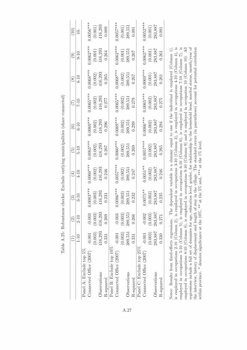
Tab
leA.25:Robustnesschecks:
Excludeoutlyingmunicipalities
(share
connected)
(1)
(2)
(3)
(4)
(5)
(6)
(7)
(8)
(9)
(10)
1-10
2-10
3-10
4-10
5-10
6-10
7-10
8-10
9-10
10-
Pan
elA:Excludetop5%
ConnectedOffice
(2007)
-0.001
-0.003
0.0083***
0.0060***
0.0063***
0.0069***
0.0065***
0.0068***
0.0062***
0.0056***
(0.003)
(0.003)
(0.003)
(0.002)
(0.002)
(0.002)
(0.002)
(0.002)
(0.001)
(0.001)
Observations
416,293
416,293
416,293
416,293
416,293
416,293
416,293
416,293
416,293
416,293
R-squared
0.331
0.269
0.231
0.246
0.267
0.296
0.277
0.265
0.264
0.089
Pan
elB:Excludetop10%
ConnectedOffice
(2007)
-0.001
-0.003
0.0086***
0.0057***
0.0060***
0.0069***
0.0065***
0.0068***
0.0062***
0.0057***
(0.003)
(0.003)
(0.003)
(0.002)
(0.002)
(0.002)
(0.002)
(0.002)
(0.001)
(0.001)
Observations
389,551
389,551
389,551
389,551
389,551
389,551
389,551
389,551
389,551
389,551
R-squared
0.331
0.266
0.232
0.247
0.269
0.299
0.279
0.267
0.267
0.091
Pan
elC:Excludetop25%
ConnectedOffice
(2007)
-0.001
-0.002
0.0075**
0.0051**
0.0057***
0.0066***
0.0065***
0.0069***
0.0062***
0.0052***
(0.003)
(0.003)
(0.003)
(0.002)
(0.002)
(0.002)
(0.002)
(0.001)
(0.001)
(0.001)
Observations
283,887
283,887
283,887
283,887
283,887
283,887
283,887
283,887
283,887
283,887
R-squared
0.330
0.271
0.235
0.246
0.265
0.294
0.275
0.261
0.261
0.091
Notes:
Resultsfrom
fixed
-effects
regressions.
Thedep
endentvariable
isadummyequalto
oneif
theindividualis
employed
(Column
1),
isem
ployedin
occupations2-10(C
olumn2),
isem
ployedin
occupations3-10(C
olumn3),
isem
ployed
inoccupations4-10(C
olumn4),
isem
ployed
inoccupations5-10(C
olumn
5),
isem
ployed
inoccupations6-10(C
olumn
6),
isem
ployed
inoccupations7-10(C
olumn
7),
isem
ployedin
occupations8-10(C
olumn8),
isem
ployedin
occupations9-10(C
olumn9)
andis
employedin
occupation10(C
olumn10).
All
regressionsincludeafullsetofdummiesforage,
educationlevel,gender,forrelationship
tothehousehold
head,maritalstatus,
month/yearof
theinterview,history
ofdisplacementandlength
ofstay
inthevillage.
Thestandard
errors
(inparentheses)accountforpotentialcorrelation
within
province.*denotessignificance
atthe10%,**
atthe5%
and,***atthe1%
level.
A.27

Tab
leA.26:Robustnesschecks:
Excludeoutlyingmunicipalities
(share
connected)
(1)
(2)
(3)
(4)
(5)
(6)
(7)
(8)
(9)
(10)
1-10
2-10
3-10
4-10
5-10
6-10
7-10
8-10
9-10
10-
Pan
elA:Excludebottom
5%
ConnectedOffice
(2007)
-0.001
-0.003
0.0089***
0.0064***
0.0064***
0.0067***
0.0062***
0.0064***
0.0063***
0.0055***
(0.003)
(0.003)
(0.003)
(0.002)
(0.002)
(0.002)
(0.002)
(0.002)
(0.002)
(0.001)
Observations
447,572
447,572
447,572
447,572
447,572
447,572
447,572
447,572
447,572
447,572
R-squared
0.331
0.271
0.232
0.246
0.269
0.297
0.277
0.265
0.264
0.088
Pan
elB:Excludebottom
10%
ConnectedOffice
(2007)
-0.001
-0.003
0.0087***
0.0060***
0.0058***
0.0061***
0.0055***
0.0059***
0.0061***
0.0055***
(0.003)
(0.003)
(0.003)
(0.002)
(0.002)
(0.002)
(0.002)
(0.002)
(0.002)
(0.001)
Observations
438,037
438,037
438,037
438,037
438,037
438,037
438,037
438,037
438,037
438,037
R-squared
0.331
0.270
0.231
0.246
0.268
0.297
0.277
0.265
0.264
0.087
Pan
elC:Excludebottom
25%
ConnectedOffice
(2007)
-0.001
-0.003
0.0095***
0.0059***
0.0060***
0.0063***
0.0056***
0.0061***
0.0065***
0.0064***
(0.003)
(0.004)
(0.003)
(0.002)
(0.002)
(0.002)
(0.002)
(0.002)
(0.002)
(0.001)
Observations
392,007
392,007
392,007
392,007
392,007
392,007
392,007
392,007
392,007
392,007
R-squared
0.331
0.269
0.228
0.243
0.266
0.294
0.274
0.262
0.261
0.083
Notes:
Resultsfrom
fixed
-effects
regressions.
Thedep
endentvariable
isadummyequalto
oneif
theindividualis
employed
(Column
1),
isem
ployedin
occupations2-10(C
olumn2),
isem
ployedin
occupations3-10(C
olumn3),
isem
ployed
inoccupations4-10(C
olumn4),
isem
ployed
inoccupations5-10(C
olumn
5),
isem
ployed
inoccupations6-10(C
olumn
6),
isem
ployed
inoccupations7-10(C
olumn
7),
isem
ployedin
occupations8-10(C
olumn8),
isem
ployedin
occupations9-10(C
olumn9)
andis
employedin
occupation10(C
olumn10).
All
regressionsincludeafullsetofdummiesforage,
educationlevel,gender,forrelationship
tothehousehold
head,maritalstatus,
month/yearof
theinterview,history
ofdisplacementandlength
ofstay
inthevillage.
Thestandard
errors
(inparentheses)accountforpotentialcorrelation
within
province.*denotessignificance
atthe10%,**
atthe5%
and,***atthe1%
level.
A.28

Table
A.27:Robustnesschecks:
Excludeoutlyingmunicipalities
(pop
ulation)
(1)
(2)
(3)
(4)
(5)
(6)
(7)
(8)
(9)
(10)
1-10
2-10
3-10
4-10
5-10
6-10
7-10
8-10
9-10
10-
Pan
elA:Excludetop5%
ConnectedOffice
(2007)
-0.002
-0.004
0.0096***
0.0065***
0.0061***
0.0066***
0.0061***
0.0064***
0.0060***
0.0050***
(0.003)
(0.003)
(0.003)
(0.002)
(0.002)
(0.002)
(0.002)
(0.002)
(0.002)
(0.001)
Observations
405,176
405,176
405,176
405,176
405,176
405,176
405,176
405,176
405,176
405,176
R-squared
0.335
0.278
0.233
0.248
0.271
0.298
0.279
0.267
0.267
0.090
Pan
elB:Excludetop10%
ConnectedOffice
(2007)
-0.001
-0.003
0.0103***
0.0080***
0.0075***
0.0075***
0.0069***
0.0071***
0.0068***
0.0050***
(0.003)
(0.003)
(0.003)
(0.002)
(0.002)
(0.002)
(0.002)
(0.002)
(0.002)
(0.001)
Observations
372,528
372,528
372,528
372,528
372,528
372,528
372,528
372,528
372,528
372,528
R-squared
0.337
0.279
0.234
0.249
0.271
0.298
0.279
0.267
0.268
0.088
Pan
elC:Excludetop25%
ConnectedOffice
(2007)
0.000
-0.004
0.0134***
0.0104***
0.0100***
0.0090***
0.0082***
0.0087***
0.0082***
0.0062***
(0.004)
(0.004)
(0.003)
(0.003)
(0.003)
(0.002)
(0.002)
(0.002)
(0.002)
(0.001)
Observations
291,874
291,874
291,874
291,874
291,874
291,874
291,874
291,874
291,874
291,874
R-squared
0.337
0.287
0.237
0.251
0.271
0.295
0.276
0.265
0.267
0.089
Notes:
Resultsfrom
fixed
-effects
regressions.
Thedep
endentvariable
isadummyequalto
oneif
theindividualis
employed
(Column
1),
isem
ployedin
occupations2-10(C
olumn2),
isem
ployedin
occupations3-10(C
olumn3),
isem
ployed
inoccupations4-10(C
olumn4),
isem
ployed
inoccupations5-10(C
olumn
5),
isem
ployed
inoccupations6-10(C
olumn
6),
isem
ployed
inoccupations7-10(C
olumn
7),
isem
ployedin
occupations8-10(C
olumn8),
isem
ployedin
occupations9-10(C
olumn9)
andis
employedin
occupation10(C
olumn10).
All
regressionsincludeafullsetofdummiesforage,
educationlevel,gender,forrelationship
tothehousehold
head,maritalstatus,
month/yearof
theinterview,history
ofdisplacementandlength
ofstay
inthevillage.
Thestandard
errors
(inparentheses)accountforpotentialcorrelation
within
province.*denotessignificance
atthe10%,**
atthe5%
and,***atthe1%
level.
A.29
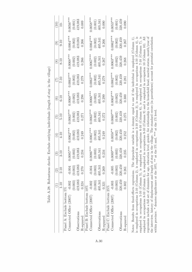
Tab
leA.28:Robustnesschecks:
Excludeoutlyingindividuals
(len
gth
ofstay
inthevillage)
(1)
(2)
(3)
(4)
(5)
(6)
(7)
(8)
(9)
(10)
1-10
2-10
3-10
4-10
5-10
6-10
7-10
8-10
9-10
10-
Pan
elA:Excludebottom
5%
ConnectedOffice
(2007)
-0.002
-0.004
0.0085***
0.0062***
0.0063***
0.0068***
0.0063***
0.0068***
0.0064***
0.0056***
(0.003)
(0.003)
(0.003)
(0.002)
(0.002)
(0.002)
(0.002)
(0.002)
(0.002)
(0.001)
Observations
419,083
419,083
419,083
419,083
419,083
419,083
419,083
419,083
419,083
419,083
R-squared
0.324
0.270
0.234
0.249
0.271
0.298
0.279
0.266
0.266
0.089
Pan
elB:Excludebottom
10%
ConnectedOffice
(2007)
-0.002
-0.004
0.0086***
0.0061***
0.0063***
0.0066***
0.0063***
0.0067***
0.0064***
0.0058***
(0.003)
(0.003)
(0.003)
(0.002)
(0.002)
(0.002)
(0.002)
(0.002)
(0.002)
(0.001)
Observations
405,341
405,341
405,341
405,341
405,341
405,341
405,341
405,341
405,341
405,341
R-squared
0.321
0.269
0.234
0.249
0.272
0.299
0.279
0.267
0.266
0.090
Pan
elC:Excludebottom
25%
ConnectedOffice
(2007)
-0.003
-0.005
0.0089***
0.0058**
0.0060***
0.0063***
0.0062***
0.0063***
0.0062***
0.0053***
(0.003)
(0.003)
(0.003)
(0.002)
(0.002)
(0.002)
(0.002)
(0.002)
(0.002)
(0.001)
Observations
320,459
320,459
320,459
320,459
320,459
320,459
320,459
320,459
320,459
320,459
R-squared
0.302
0.261
0.235
0.252
0.275
0.300
0.281
0.268
0.267
0.090
Notes:
Resultsfrom
fixed
-effects
regressions.
Thedep
endentvariable
isadummyequalto
oneif
theindividualis
employed
(Column
1),
isem
ployedin
occupations2-10(C
olumn2),
isem
ployedin
occupations3-10(C
olumn3),
isem
ployed
inoccupations4-10(C
olumn4),
isem
ployed
inoccupations5-10(C
olumn
5),
isem
ployed
inoccupations6-10(C
olumn
6),
isem
ployed
inoccupations7-10(C
olumn
7),
isem
ployedin
occupations8-10(C
olumn8),
isem
ployedin
occupations9-10(C
olumn9)
andis
employedin
occupation10(C
olumn10).
All
regressionsincludeafullsetofdummiesforage,
educationlevel,gender,forrelationship
tothehousehold
head,maritalstatus,
month/yearof
theinterview,history
ofdisplacementandlength
ofstay
inthevillage.
Thestandard
errors
(inparentheses)accountforpotentialcorrelation
within
province.*denotessignificance
atthe10%,**
atthe5%
and,***atthe1%
level.
A.30

Table
A.29:Robustnesschecks:
Excludesomeagegroups
(1)
(2)
(3)
(4)
(5)
(6)
(7)
(8)
(9)
(10)
1-10
2-10
3-10
4-10
5-10
6-10
7-10
8-10
9-10
10-
Pan
elA:Age<
63ConnectedOffice
(2007)
-0.000
-0.000
0.0084***
0.0062***
0.0061***
0.0063***
0.0058***
0.0062***
0.0061***
0.0054***
(0.003)
(0.003)
(0.003)
(0.002)
(0.002)
(0.002)
(0.002)
(0.002)
(0.002)
(0.001)
Observations
408,386
408,386
408,386
408,386
408,386
408,386
408,386
408,386
408,386
408,386
R-squared
0.338
0.275
0.236
0.251
0.272
0.302
0.281
0.268
0.267
0.090
Pan
elB:Age
>22
ConnectedOffice
(2007)
-0.002
-0.003
0.0092***
0.0063***
0.0068***
0.0071***
0.0067***
0.0070***
0.0068***
0.0060***
(0.003)
(0.003)
(0.003)
(0.002)
(0.002)
(0.002)
(0.002)
(0.002)
(0.002)
(0.001)
Observations
406,311
406,311
406,311
406,311
406,311
406,311
406,311
406,311
406,311
406,311
R-squared
0.329
0.265
0.243
0.256
0.279
0.309
0.288
0.275
0.274
0.092
Pan
elC:Age>
22andAge<
63
ConnectedOffice
(2007)
-0.000
-0.001
0.0091***
0.0066***
0.0068***
0.0068***
0.0063***
0.0067***
0.0069***
0.0060***
(0.003)
(0.003)
(0.003)
(0.002)
(0.002)
(0.002)
(0.002)
(0.002)
(0.002)
(0.001)
Observations
360,353
360,353
360,353
360,353
360,353
360,353
360,353
360,353
360,353
360,353
R-squared
0.335
0.267
0.248
0.261
0.283
0.315
0.293
0.279
0.278
0.094
Notes:
Resultsfrom
fixed
-effects
regressions.
Thedep
endentvariable
isadummyequalto
oneif
theindividualis
employed
(Column
1),
isem
ployedin
occupations2-10(C
olumn2),
isem
ployedin
occupations3-10(C
olumn3),
isem
ployed
inoccupations4-10(C
olumn4),
isem
ployed
inoccupations5-10(C
olumn
5),
isem
ployed
inoccupations6-10(C
olumn
6),
isem
ployed
inoccupations7-10(C
olumn
7),
isem
ployedin
occupations8-10(C
olumn8),
isem
ployedin
occupations9-10(C
olumn9)
andis
employedin
occupation10(C
olumn10).
All
regressionsincludeafullsetofdummiesforage,
educationlevel,gender,forrelationship
tothehousehold
head,maritalstatus,
month/yearof
theinterview,history
ofdisplacementandlength
ofstay
inthevillage.
Thestandard
errors
(inparentheses)accountforpotentialcorrelation
within
province.*denotessignificance
atthe10%,**
atthe5%
and,***atthe1%
level.
A.31

.02
.025
.03
.035
.04
.045
Pr(
Man
ager
ial J
ob=
1)
-10 -5 0Vote Margin
Related to Losers (2007) Related to Losers (2010)
Figure A.1: Non-parametric estimates of the probability of being employed in a managerialposition
A.32

-.03
-.02
-.01
0.0
1.0
2B
eta
0-5 5-10 10-15 15-20Sample - Vote Margin (percent)
95% Confidence Interval Point Estimates
Figure A.2: Estimated Effects by Loss Margin
A.33


![CSAE Working Paper WPS/2014-33 · individual characteristics affects the level and dynamics of cooperation in human groups [Ledyard, 1995, Reuben and Riedl, 2013]. Social networks](https://static.fdocuments.in/doc/165x107/5e7279d5dcd1b0343c371bcf/csae-working-paper-wps2014-33-individual-characteristics-aiects-the-level-and.jpg)