CS 547: Sensing and Planning in Robotics

Gaurav S. Sukhatme

Computer Science

Robotic Embedded Systems Laboratory

University of Southern California

gaurav@usc.edu

http://robotics.usc.edu/~gaurav

(Slides adapted from Thrun, Burgard, Fox book slides)

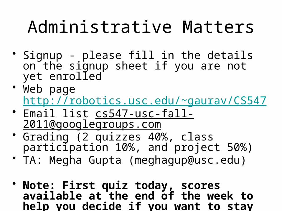
Administrative Matters

• Signup - please fill in the details on the signup sheet if you are not yet enrolled

• Web page http://robotics.usc.edu/~gaurav/CS547• Email list cs547-usc-fall-2011@googlegroups.com• Grading (2 quizzes 40%, class participation 10%,

and project 50%)• TA: Megha Gupta (meghagup@usc.edu)

• Note: First quiz today, scores available at the end of the week to help you decide if you want to stay in the class

Project and Textbook

• Project– Small teams or individual projects– Equipment (ROS, PR2)

• Book– Probabilistic Robotics (Thrun, Burgard, Fox)– Available at the Bookstore

I expect you to

• come REGULARLY to class• visit the class web page FREQUENTLY• read email EVERY DAY• SPEAK UP when you have a question• START EARLY on your project

• If you don’t– the likelihood of learning anything is small– the likelihood of obtaining a decent grade is small

In this course you will

– Learn how to address the fundamental problem of robotics i.e. how to combat uncertainty using the tools of probability theory

– Explore the advantages and shortcomings of the probabilistic method

– Survey modern applications of robots– Read some cutting edge papers from the

literature

Syllabus and Class Schedule• 8/22 Introduction and probability theory background• 8/29 Bayesian filtering• 9/5 (no class) Labor Day • 9/12 PR2 and ROS tutorial• 9/19 Sensor models and perception• 9/26 Quiz 1 (Gaurav and Megha at IROS)• 10/3 Action models • 10/10 Bayesian filtering revisited: the Kalman filter & Particle

filtering• 10/17 The Markov decision process• 10/24 The partially observable Markov decision process• 10/31 Interim project updates (short presentations and demos)• 11/7 Mixture models and the Expectation-Maximization

algorithm• 11/14 Quiz 2 (Gaurav on travel) and extended office hours• 11/21 Extended office hours• 11/28 Final project presentations

Robotics Yesterday

Robotics Today

Robotics Tomorrow?

What is Robotics/a Robot ?

• Background– Term robot invented by Capek in 1921 to mean a

machine that would willing and ably do our dirty work for us

– The first use of robotics as a word appears in Asimov’s science fiction

• Definition (Brady): Robotics is the intelligent connection of perception to action

• History (Wikipedia entry is a reasonable intro)

Trends in Robotics Research

Reactive Paradigm (mid-80’s)• no models• relies heavily on good sensing

Probabilistic Robotics (since mid-90’s)• seamless integration of models and sensing• inaccurate models, inaccurate sensors

Hybrids (since 90’s)• model-based at higher levels• reactive at lower levels

Classical Robotics (mid-70’s)• exact models• no sensing necessary

Robots are moving away from factory floors to Entertainment, Toys, Personal service. Medicine, Surgery, Industrial automation (mining, harvesting), Hazardous environments (space, underwater)

Tasks to be Solved by Robots Planning Perception Modeling Localization Interaction Acting Manipulation Cooperation ...

Uncertainty is Inherent/Fundamental

• Uncertainty arises from four major factors:– Environment is

stochastic, unpredictable

– Robots actions are stochastic

– Sensors are limited and noisy

– Models are inaccurate, incomplete

Odometry Data

Range Data

Probabilistic Robotics

Explicit representation of uncertainty using the calculus of probability theory

• Perception = state estimation• Action = utility optimization

Advantages and Pitfalls

• Can accommodate inaccurate models• Can accommodate imperfect sensors• Robust in real-world applications• Best known approach to many hard

robotics problems• Computationally demanding• False assumptions• Approximate

Pr(A) denotes probability that proposition A is true.

•

•

•

Axioms of Probability Theory

1)Pr(0 ≤≤ A

1)Pr( =True

)Pr()Pr()Pr()Pr( BABABA ∧−+=∨

0)Pr( =False

A Closer Look at Axiom 3

B

BA∧A BTrue

)Pr()Pr()Pr()Pr( BABABA ∧−+=∨

Using the Axioms

)Pr(1)Pr(

0)Pr()Pr(1

)Pr()Pr()Pr()Pr(

)Pr()Pr()Pr()Pr(

AA

AA

FalseAATrue

AAAAAA

−=¬−¬+=

−¬+=¬∧−¬+=¬∨

Discrete Random Variables• X denotes a random variable.

• X can take on a finite number of values in {x1, x2, …, xn}.

• P(X=xi), or P(xi), is the probability that the random variable X takes on value xi.

• P( ) is called probability mass function.

• E.g. 02.0,08.0,2.0,7.0)( =RoomP

.

Continuous Random Variables• X takes on values in the continuum.

• p(X=x), or p(x), is a probability density function.

• E.g.

∫=∈b

a

dxxpbax )(]),[Pr(

x

p(x)

Joint and Conditional Probability

• P(X=x and Y=y) = P(x,y)

• If X and Y are independent then

P(x,y) = P(x) P(y)

• P(x | y) is the probability of x given y

P(x | y) = P(x,y) / P(y)

P(x,y) = P(x | y) P(y)

• If X and Y are independent then

P(x | y) = P(x)

Law of Total Probability

∑=y

yxPxP ),()(

∑=y

yPyxPxP )()|()(

∑ =x

xP 1)(

Discrete case

∫ =1)( dxxp

Continuous case

∫= dyypyxpxp )()|()(

∫= dyyxpxp ),()(

Reverend Thomas Bayes, FRS (1702-1761)

Clergyman and mathematician who first used probability inductively and established a mathematical basis for probability inference

Bayes Formula

evidence

prior likelihood

)(

)()|()(

)()|()()|(),(

⋅==

⇒

==

yPxPxyP

yxP

xPxyPyPyxPyxP

Conditioning

• Total probability:

• Bayes rule and background knowledge:

)|(

)|(),|(),|(

zyP

zxPzxyPzyxP =

∫= dzyzPzyxPyxP )|(),|()(

Simple Example of State Estimation• Suppose a robot obtains measurement z• What is P(open|z)?

Causal vs. Diagnostic Reasoning

• P(open|z) is diagnostic.• P(z|open) is causal.• Often causal knowledge is easier to

obtain.• Bayes rule allows us to use causal

knowledge:

)()()|(

)|(zP

openPopenzPzopenP =

count frequencies!

Example

• P(z|open) = 0.6 P(z|open) = 0.3• P(open) = P(open) = 0.5

67.03

2

5.03.05.06.0

5.06.0)|(

)()|()()|(

)()|()|(

==⋅+⋅

⋅=

¬¬+=

zopenP

openpopenzPopenpopenzPopenPopenzP

zopenP

• z raises the probability that the door is open.

Combining Evidence

• Suppose our robot obtains another observation z2.

• How can we integrate this new information?

• More generally, how can we estimateP(x| z1...zn )? (next lecture)

Example: Second Measurement

• P(z2|open) = 0.5 P(z2|open) = 0.6

• P(open|z1)=2/3

625.08

5

31

53

32

21

32

21

)|()|()|()|(

)|()|(),|(

1212

1212

==⋅+⋅

⋅=

¬¬+=

zopenPopenzPzopenPopenzPzopenPopenzP

zzopenP

• z2 lowers the probability that the door is open.

Actions

• Often the world is dynamic since– actions carried out by the robot,– actions carried out by other agents,– or just the time passing by

change the world.

• How can we incorporate such actions?

Typical Actions

• The robot turns its wheels to move• The robot uses its manipulator to grasp an

object

• Actions are never carried out with absolute certainty.

• In contrast to measurements, actions generally increase the uncertainty.

Modeling Actions

• To incorporate the outcome of an action u into the current “belief”, we use the conditional pdf

P(x|u,x’)

• This term specifies the pdf that executing u changes the state from x’ to x.

Example: Closing the door

State Transitions

P(x|u,x’) for u = “close door”:

If the door is open, the action “close door” succeeds in 90% of all cases.

Integrating the Outcome of Actions

∫= ')'()',|()|( dxxPxuxPuxP

∑= )'()',|()|( xPxuxPuxP

Continuous case:

Discrete case:

Example: The Resulting Belief

)|(1161

83

10

85

101

)(),|(

)(),|(

)'()',|()|(

1615

83

11

85

109

)(),|(

)(),|(

)'()',|()|(

uclosedP

closedPcloseduopenP

openPopenuopenP

xPxuopenPuopenP

closedPcloseduclosedP

openPopenuclosedP

xPxuclosedPuclosedP

−=

=∗+∗=

+=

=

=∗+∗=

+=

=

∑

∑

Next Lecture

• Bayesian Filtering– The Markov assumption– A recursive filter from Bayes rule– Examples

)()|(

),,|()|(

),,|(

),,|()|(),,|(

...1...1

11

11

111

xPxzP

zzxPxzP

zzzP

zzxPxzPzzxP

ni

in

nn

nn

nnn

∏=

−

−

−

=

=

=

η

η K

KK

K