CRT2 - Water and Sewer Infrastructure, Operations, … and Sewer Infrastructure, Operations, and...

2017 Annual Conference & Exposition

CRT2 - Water and Sewer Infrastructure, Operations, and Maintenance

June 12, 2017 Philadelphia, Pennsylvania

Water and Sewer Infrastructure, Operations, and Maintenance

Course 2 in the Public Officials Certificate Program

Instructor: Frederick Bloetscher, Ph.D., P.E.

2

Course 2 What did you learn in Course 1?

3

My Goals of Class

• Help YOU Gain an Understanding of:

–Operations/Maintenance

–Asset Management and Maintenance

–Programs You Need

–Finance

–Capital Planning

So Now That We Have Water,How Do We Make it Safe?

Let’s Look in More Detail at Processes…

High-Quality Groundwater Treatment Regime

6

Chlorination Distribution System

Well

Source: Bloetscher, 2008

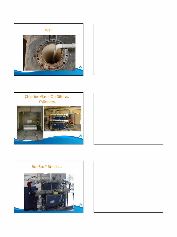
Well

Chlorine Gas – On-Site vs. Cylinders

8

But Stuff Breaks…

9

Chlorine Bleach System

10

High Service Pumps

High-Quality Surface Water Treatment Regime

12

Surface Water

Pipe

Filtration



High Quality Lake

Flocculator

Pressure Filters

Sand Filters

Chemical Mix Systems

17Source: Bloetscher, 2008

Medium-Quality Groundwater Treatment Regime

18

Lime

Lime Softening

Filtration


Well


Lime Slurry Mixers

19


Lime Softening and Filters

20


Lime Softening


Lime Softening Reactor

On Top of the Unit

23

Lime Softening

Filters


Medium-Quality Surface Water Treatment Regime

26

Surface Water Alum

Flocculation

Clarifier/Settling

Filtration

Chlorination

Distribution System

Chlorine

Contact


27

Flocculation Basin

How Settling Tanks Work…

28

Velocity

vo

Mix end – may be turbulent

Exit turbulence

WeirWater surface

Settled particles


Sand Filters

Low-Quality Groundwater Treatment Regime

30

Lime

Lime Softening

CO2

Filtration

Air-Strippers

Well Draft Air



Low-Quality Surface Water Treatment Regime

31

Surface Water Alum

Flocculation

Clarifier/Settling

Carbon (GAC/PAC)

Filtration

Draft Air

Distribution System

Chlorine

Contact


MIEX System

Aeration Concept

33

Media

Water Down

Air Blown Up

Cartridge Filter Housing

Cartridge Filters

Used Cartridge Filter

Membranes

37

Membrane System

Membranes

Secondary Wastewater Treatment

40

Bar Screen

Aeration Basin

Chlorination

Disposal

Primary

Clarifer

Secondary

Clarifier

Chlorine

Contact


Used Membranes

Wastewater Treatment

42

Fine Bubble Aeration System

Contact Stabilization Plant

44

Wastewater Treatment

45

Empty…

46

Membrane Bioreactor

Membrane Bioreactor

Membrane Bioreactor

Advanced Secondary Wastewater Treatment (Reuse)

50

Filters

Bar Screen

Aeration Basin

Chlorine

Disposal

Primary

ClariferSecondary

Clarifier

Chlorine

Contact


Reuse Filters and Chlorination Basin

51

Reuse Effluent Pumping and Tank

52

Advanced Wastewater Treatment

53

Filters

Bar Screen

Aeration Basin

Nitrification

Chlorination

Disposal

Primary

Clarifer Secondary

Clarifier

Denitrif.

Tank

Chlorine

Contact

Dechlor-

rination


Anoxic Zone

54

Ultraviolet Light

Full Treatment

56

Filters

Bar Screen

Aeration Basin

Nitrification

CL Disposal

Primary

Clarifer

Second.

Clarifier

Denitrif.

Tank

CL

ContactDechlor

GACRO

Background: Standard of CareMulti Barrier Approach

• Microfiltration

• Reverse Osmosis

• Ultraviolet Advanced Oxidation

Ultraviolet Advanced Oxidation

Reverse Osmosis

Microfiltration

California Water Factory 21Groundwater Replenishment System

Process Flow Schematic

Phase II

Phase I

SP-2 After Microfilter SP-3 After

Reverse Osmosis

SP-4 After UV/AOP

SP-1 Influent to Pilot Plant

SP-1

SP-2

SP-3

SP-4

INFLUENT

Pilot Plant

Pembroke Pines Pilot Plant(Looking Northwest)

Pilot StudyMaximize the Recovery of the RO

• Configurations

Two stage 2:1 → 75% recovery

Three stage 2:1:1 → 82% recovery

Two Stage 2:1

Third Stage 1:1

Comparison of the permeate and third stage concentrate

Membrane Properties

Summary of Membrane Operating Parameters

Parameter DOW FilmTec Hydranautics Koch

Membrane Type Polyamide TFC Composite Polyamide TFC Polyamide

Maximum Operating Temperature 113 °F 113 °F 113 °F

Maximum Pressure Drop 15 psi 10 psi 10 psi

pH Range, Continuous Operation 2 - 11 2 - 11 4 - 11

pH Range, Short-Term Cleaning 1 - 13 1 - 13 2.5 - 11

Maximum Feedwater SDI 5.0 5.0 5.0

Free Chlorine Tolerance < 0.1 ppm < 0.1 ppm < 0.1 ppm

Nominal Active Surface Area 78 ft2 80 ft

2 85 ft

2

Recovery Rate 15% 15% 15%

Permeate Flow Rate: 2,400 gpd 2,000 gpd 2,370 gpd

Maximum Feedwater Turbidity 1.0 NTU 0.2 NTU

Stabilized Salt Rejection 99.5% 99.6% 99.55%

Membrane Specified BW30-4040 ESPA2-LD-4040 TFC-4040-HR

DOW Filmtec Test Operating Conditions: 2,000 ppm NaCl, 225 psig, 77°F, and 15% recovery

Hydranautics Test Operating Conditions: 1,500 ppm NaCl, 225 psig, 77°F , and 15% recovery

Koch Test Operating Conditions: 2,000 ppm NaCl, 225 psig, 77°F, and 15% recovery

Pilot StudyPost Treatment Stabilization

• pH

• Hardness

• Mineral content

• DO

• ORP

Stabilization Techniques

• Sodium hydroxide

• Hydrated lime

• Limestone filter

• Kiln dust

• Sodium metabisulfate

Pilot Study

Florida Atlantic University Spike Test

Group Overall % Removal

Pharmaceuticals 99.78%

Antibacterials 99.99%

Steroids & Hormones 99.95%

Protein Degradation Products 99.99%

Flame Retardants 99.89%

ESOC Treatment Evaluation

Trojan Technologies Spike Test

Parameter Goal Removal

NDMA 1.2-log (93.7%) > 2.76-log

1,4-dioxane 0.5-log (68.4%) > 1.83-log

Constituents SpikedChemical CAS MW Solubility pKa

Acetaminophen 130-90-2 151 14 mg/ml 9.51

Ibuprofen 51146-56-6 206 0.06 mg/ml 4.4

Estrone 53-16-7 270 1.30 mg/L 10.9

Triclosan 3380-34-5 289 0.012 g/L(1) 9.95(2)

Carbamazepine 298-46-4 236 17.7 mg/L 13.9

NDMA(3) 62-75-9 74 29 g/100 ml 3.52

1,4-D (Dioxane)(3) 123-91-1 88 ∞ N/A

TCEP 115-96-8 285 7.82 g/L N/A

Spiking the Water

Spike Removal Values

Spike Test #1 #2 #3 #1 #2 #3

Pharmaceuticals

Acetaminophen 91.30% 96.88% 97.27% 99.92% 98.32% 99.95%

Carbamazepine 85.00% 99.97% 99.91% 99.93% 99.98% 99.97%

Ibuprofen 85.37% 100.00% 99.92% 100.00% 100.00% 99.98%

Antibacterials

Triclosan 27.94% 97.50% 99.98% 100.00% 100.00% 100.00%

Steroids/Hormones

Estrone 67.70% 98.84% 99.99% 99.87% 100.00% 100.00%

Protein Degradation

N-Nitrosodimethylamine (NDMA) 62.77% 48.29% 39.01% 99.96% 99.90% 100.00%

Flame Retardants (Chlorinated Phosphates)

Tris(2-chloroethyl)phosphate (TCEP) 73.97% 99.77% 99.80% 99.89% 100.00% 99.83%

Other

1,4-D (Dioxane) 97.84% 94.28% 96.86% 99.89% 94.17% 97.80%

Average 73.99% 91.94% 91.59% 99.93% 99.05% 99.69%

Green indicates 3 log target is achieved

Percent Removal

Post RO Post UV

Study Results

• One of the goals of this study was to prove a3-Log (99.9%) reduction using an RO/UV/AOPtreatment train.

• Such reduction was obtained for all chemicalsexcept TCEP and 1,4-Dioxane which had acombined percent removal equivalent to99.83 and 97.80 percent respectively.

Orange County Does It

Big Springs Drinks It

Disposal of Residuals/Sludge

71

Belt Press

Water Distribution System Consists of:

• Extensive underground systems of varyingtypes of:

–Pipe

–Valves, hydrants, and otherappurtenances

–Meters and service lines

• Various storage and pumping programs

• Maintenance of all parts on an ongoingbasis

73

Piping for Water - Issues to Consider

• Strength

• Exposure

• Chemicals/contaminant exposure

• Constructability

• Availability

74

For Example

• High tension forces = steel

• Compression forces = concrete

• Corrosive environments = avoid steel

• Dissimilar metals = always avoid

• Salts = Steel will corrode – need highergrades steel or plastic

• Active biology = not steel

75

Ductile Iron

76

77

PVC Pipe

SDR 21

Schedule 40 PVC

HDPE or MDPE

78

PVC Pipe

79

HDPE

80

Insulated Pipe

81

Reinforced Concrete (Pressurized)

82

Department of Civil Engineering • F. Bloetscher, Ph.D., P.E. • ENV 4514 • Fall 2007

Recommended Water Distribution Programs

• Leak detection

• Water loss records

• Work order to track repairs, pipe condition

• System mapping

• Replacement programs

• Valve exercise & fire hydrant test programs

85Source: AWWA

Service Line and Meter

Storage Methods

86

Why Storage is Needed

87

Average Daily Flow

Pumping Out > Production

Pumping Out < Production (tanks fill)

Midnight Noon Midnight

Time of Day

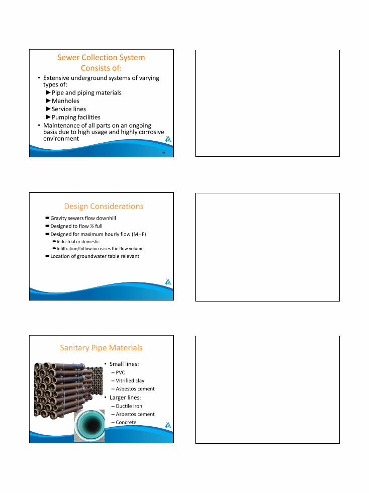
Sewer Collection System Consists of:

• Extensive underground systems of varyingtypes of:►Pipe and piping materials►Manholes►Service lines►Pumping facilities

• Maintenance of all parts on an ongoingbasis due to high usage and highly corrosiveenvironment

88

Design ConsiderationsGravity sewers flow downhill

Designed to flow ½ full

Designed for maximum hourly flow (MHF)

Industrial or domestic

Infiltration/Inflow increases the flow volume

Location of groundwater table relevant

Sanitary Pipe Materials

• Small lines:

– PVC

– Vitrified clay

– Asbestos cement

• Larger lines:

– Ductile iron

– Asbestos cement

– Concrete

Types of Manholes?

• Doghouse Precast

• Drop

Brick

Manhole Design

92

bench

Source: City of Austin, TX

Stuff That Shouldn’t Be

93

http://www.fi-hoff.com/photos/newspecialmh.JPG

Sewer Higher Than Water Sales?

0

1

2

3

4

5

6

Dec-99 Apr-01 Sep-02 Jan-04 May-05 Oct-06 Feb-08

Month

AD

F (

MG

D)/

Ra

infa

ll i

n I

nc

he

s

W-ADF

S-ADF

Inflow/Infiltration

95

Inflow/Infiltration

96

Flows Get Worse With Time

Inflow: Rainwater

Infiltration: Groundwater

What is

Inflow and Infiltration?

Rain and High Groundwater AffectsRain and High Groundwater Affects

Wastewater Collection SystemWastewater Collection System

Infiltration/Inflow (I/I)

InfiltrationGroundwater that enters the sewer through defective

pipes, joints, connections, & manholes

InflowStormwater discharged directly into sewers from roof

drains and stormwater runoff

Both overloads collection systems & reduces treatment efficiencyFunction of age

I/I = 0.009 – 0.9 m3/d∙mm∙km (typically)

0.00

2.00

4.00

6.00

8.00

10.00

12.00

14.000

500,000

1,000,000

1,500,000

2,000,000

2,500,000

3,000,000

3,500,000

4,000,000

Se

we

r Fl

ow

Date

Flow (Gallons)

Rainfall

Rain

fall

Flow Data vs. Rainfall

Inflow = Rain

Sewer Flows v. RainfallWe can see…..INFLOW!!!

0

5

10

15

20

25

Dec-99 Apr-01 Sep-02 Jan-04 May-05 Oct-06 Feb-08

Month

AD

F (

MG

D)/

Rai

nfa

ll in

Inch

es

S-ADF

Rainfall

WATERWAY

FOOTING

DRAIN SANITARY

SEWER

STORMWATER

SEWER

SUMP

PUMP

HOUSE

SEWER

(LATERAL)

DOWN-

SPOUT

STREET

INLET

INFILTRATION

STORMWATER

CONNECTIONS

ALLOW INFLOW SANITARY SEWERS

OVERFLOW TO

WATERWAYS

BASEMENT

BACKUP

Inflow =>Sanitary Sewer Overflow

Sanitary Sewer Overflow

• Sewer flow peaks during rain events.

• The size of the storm event matters. A larger storm event will create more inflow.

• During storm events, wastewater flow is linearly related to rainfall.

• Based on an analysis of flow vs. rainfall graphs from pre and post construction activities inflow reduction will be calculated.

Inflow

Broken Pipe = Infiltration…

Broken Pipe

Leaky Pipe

Pipeline Leak Repair

Lift Station, Generator and Control Box

108

Dirty Wet Well

109

“Clean” Wet Well

110

111

True Inflow vs Infiltration

112

Vacuum Sewer Design

113

A traditional gravity line carries wastewater from the customer to a valve pit package.

When 10 gallons of wastewater collects in the sump, the valve opens and differential pressure propels the contents into the vacuum main.

Wastewater travels at 15 to 18 fps in the vacuum main, which is laid in a sawtooth fashion to insure adequate vacuum levels at the end of each line.

Wastewater enters the collection tank. When the tank fills to a predetermined level, sewage

pumps transfer the contents to the treatment plant via a force

main.

Vacuum pumps cycle on and off as needed to maintain a constant level of vacuum on the entire collection system.

Source: Partlow, 2007

Ongoing Sewer Collection System Maintenance Programs

• Infiltration and inflow correction

• Monitor pumpage

• Work orders to track repairs, pipe condition

• System mapping

• Repair and replacement programs

114

Deterioration of Infrastructure

Maint

Cost

Pipelines

Mechanical Equipment

Time

Rehab Provides Only So Much

116

Percent Refurbish 1

of Original Refurbish 2

Value

(Present Initial Lifecycle

Worth)

Extended Life

Time

Note - refurbishment may occur later in life before full devaluation takes place.

Refurbishment never reaches initial condition.

Extension of life of asset decreases with each refurbishment.

What Are Maintenance Concerns?

• Age• Structural

breakdowns• Wear• Deterioration due to

– Corrosion damage –Water quality–Water stability–Material breakdown

So What Creates the Problem?

• Technology changes

• Use Changes/repurpose

• Environmental effects–Galvanic action/corrosion

–Unstable water/solutions

–Biofouling

• Failure to maintain/inspect/repair

118

What Is Asset Management?

• Business process and a decision-makingframework that covers an extended timehorizon, draws from economics as well asengineering, and considers a broad rangeof assets

• Asset management is part of maintenance

• And part of management

Asset Management is Not New

• What changed?–Construction to

operations

–Materialinstallation torepair

• Not glamorous likeconstruction

Asset Management Has Come of Age Because of…

• Condition of the infrastructure

• Increased potential for water andsewer system disruptions

• Overflows and breaks that disruptservice

• Changes in public expectations

• Advances in technology

Issues

• Certainty – this is what engineers like todeal with, but stationarity is “dead”

• Risk – probability of things happening ornot

• Uncertainty – things you don’t haveanswers to – may be the largest data

Process

Determine Goals &

Objectives

Inventory of Assets

System Review & Assessment

AMP

ImplementationQuality

Assurance

Performance Feedback

123

What Does All This Cost?????

• It is ongoing work

• It cannot be delayed indefinitely

• It cannot be ignored

• Delays = dollars later

• Failure is not an option

• Water system >$1 trillion over 20 years

124

$

Minimum Requirements

• Adaptable

• Efficient

• Practical

• Decisionsupported

• Good feedback

Condition Index• Variety of Factors

• Yields Result

• If we know the incident, we can find theweights

• CI = w1C1+w2C2+w3C3+w4C4+…wiCi

• Where:

– CI = Condition index

– W = weighting factor

– C is condition factor

Concept

• Linear constraints are equalities withthe following form:

• Or inequalities with the followingform:

127

1332211 ... bxaxaxaxa niniii

1332211 ... bxaxaxaxa niniii

1)( dxxf

128

If You Don’t Have Much Data…Bayesian Methods Might Work

Unconditional Probability Density Function

dpxpxp )()|()(

129

where p(x) and p(q) are completely different and independent functions and the function p(q) is the prior distribution

absolute or unconditional probability density function p(x) on X is the underlying distribution found through curve-fitting

What is p(x)? Or b?

It must be a measurable incident or response

So We Need to Know What That Response is

• Water main breaks?

• Sewer breaks? Overflows?

• Stormwater??

• Irrigation breaks?

132

Step 1 Create a table of assets Step 2 Create columns for the variables for which you have data Step 3 Categorical and numerical variable do not provide appropriate comparisons; hence the need to alter the categorical variables to absence/presence variables. Step 4 Summarize the statistics for the variables. .Step 5 Develop a linear regression to determine factors associated with each and the amount of influence that each exerts. Step 6 Identify the predictive equation. Step 7 The equation can then be used to predict the number ofbreaks going forward.Step 8 Finally the data can be used to predict where the breaksmight occur in the future based on the past

Let’s Look at a Water System• Pipe size

• Estimate age form aerials, as-builts, development patterns, etc.

• Condition based some on age, as-builts, field crews

• Soils (USDA), can assume better soil put back in

• Pressure (55 psi)

• Traffic (road it is on)

• Trees (GoogleEarth – going out and looking)

• Rumor (what do crews think)

• On-site analysis (over all the others)

• Others….

133

Step 1 - Create a Spreadsheet of Assets

Asset Diameter

water main 2

water main 2

water main 2

water main 2

water main 4

water main 6

water main 6

water main 6

water main 6

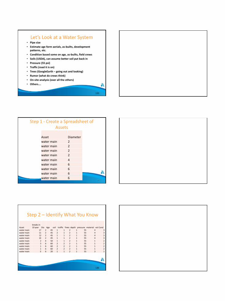
Step 2 – Identify What You Know

Assetbreaks in 10 year Dia Age soil traffic Trees depth pressure material est Cond

water main 17 2 45 1 1 2 1 55 4 3water main 11 2 45 2 1 2 1 55 4 3water main 12 2 45 1 1 2 1 55 4 3water main 10 2 45 1 1 2 1 55 4 3

water main 2 4 50 1 1 2 1 55 1 2water main 3 6 60 2 2 2 1 55 1 2water main 1 6 60 2 2 2 1 55 1 2water main 1 6 60 2 2 2 1 55 1 2water main 0 6 20 1 1 2 1 55 3 1

135

AssumptionsKeySoil 1 = sand 2 = muckDepth 1 =<6 2>6

Trees1 = no, 2 = yes

Traffic 1= low 2 = high

Material1 = Di 2 = GI 3 =C900 4 = AC 5 = hdpe

Est Cond1= good 2 = fair 3 = poor

136

Step 3 – Convert Descriptive Info to Numerical

Asset

breaks in

10 year Dia Age Sand Clay

Low

Traffic

Heavy

Traffic Trees

no

trees

shallow

unde 6

deep

bury pressure

DIP

CI GI PVC AC

HDP

E

water main 17 2 45 1 0 1 0 1 0 1 0 55 0 0 0 1 0

water main 11 2 45 0 1 1 0 1 0 1 0 55 0 0 0 1 0

water main 12 2 45 1 0 1 0 1 0 1 0 55 0 0 0 1 0

water main 10 2 45 1 0 1 0 1 0 1 0 55 0 0 0 1 0

water main 2 4 50 1 0 1 0 1 0 1 0 55 1 0 0 0 0

water main 3 6 60 0 1 0 1 1 0 1 0 55 1 0 0 0 0

water main 1 6 60 0 1 0 1 1 0 1 0 55 1 0 0 0 0

water main 1 6 60 0 1 0 1 1 0 1 0 55 1 0 0 0 0

water main 0 6 20 1 0 1 0 1 0 1 0 55 0 0 1 0 0

Step 4 – Summary Statistics

138

Table 4 Summary statistics:

Variable

Observa-

tions

Obs. with

missing data

Obs. without

missing data

Mini-

mum

Maxi-

mum Mean

Std.

deviation

breaks in 10 year 93 0 93 0.000 17.000 1.398 2.949

Dia 93 0 93 1.000 16.000 5.011 3.255

Age 93 0 93 5.000 60.000 29.194 18.212

Sand 93 0 93 0.000 1.000 0.946 0.227

Clay 93 0 93 0.000 1.000 0.054 0.227

Low Traffic 93 0 93 0.000 2.000 0.968 0.231

Heavy Traffic 93 0 93 0.000 1.000 0.043 0.204

Trees 93 0 93 0.000 1.000 0.903 0.297

no trees 93 0 93 0.000 1.000 0.215 0.413

shallow under 6 ft

deep 93 0 93 0.000 1.000 0.849 0.360

deep bury 93 0 93 0.000 1.000 0.032 0.178

pressure 93 0 93 55.000 65.000 55.323 1.616

Ductile 93 0 93 0.000 1.000 0.419 0.496

GI 93 0 93 0.000 1.000 0.054 0.227

PVC 93 0 93 0.000 1.000 0.247 0.434

AC 93 0 93 0.000 1.000 0.065 0.247

HDPE 93 0 93 0.000 5.000 1.075 2.065

Step 5 – Linear Regression

• Means to derive an equation and fitfor the data

• Highlights how much the variability isdefined by the data

139

Steps 5&6 – Linear Regression and Model Parameters

Model parameters:

Source Value

Standard

error t Pr > |t|

Lower bound

(95%)

Upper bound

(95%)

Intercept -12.355 6.805 -1.816 0.073 -25.901 1.190

Dia -0.489 0.102 -4.795 < 0.0001 -0.692 -0.286

Age 0.008 0.012 0.725 0.471 -0.015 0.032

Sand 3.144 0.891 3.528 0.001 1.370 4.918

Clay 0.000 0.000

Low Traffic 1.151 1.546 0.744 0.459 -1.926 4.227

Heavy Traffic 5.961 2.107 2.830 0.006 1.768 10.154

Trees -2.819 1.236 -2.280 0.025 -5.280 -0.359

no trees 0.297 1.134 0.262 0.794 -1.959 2.554

shallow under

6 0.580 1.034 0.561 0.576 -1.478 2.639

deep bury 0.000 0.000

pressure 0.194 0.119 1.625 0.108 -0.044 0.431

Ductile 2.342 0.640 3.658 0.000 1.068 3.617

GI 5.473 0.598 9.151 < 0.0001 4.282 6.663

PVC 3.229 0.717 4.501 < 0.0001 1.801 4.657

AC 12.428 0.757 16.408 < 0.0001 10.920 13.935

HDPE 0.000 0.000

Step 6 – Impact of Model Parameters

Dia

Ag

e

San

d

Cla

y Lo

w T

raff

ic

Hea

vy T

raff

ic

Tre

es

no

tre

es

shal

low

un

de

6

dee

p b

ury

pre

ssu

re Du

ctile

GI P

VC

AC

HD

PE

-1

-0.5

0

0.5

1

1.5

Sta

nd

ard

ize

d c

oe

ffic

ien

ts

Variable

breaks in 10 year / Standardized coefficients(95% conf. interval)

Step 7 – Predictions by Observation

-4.5 -3.5 -2.5 -1.5 -0.5 0.5 1.5 2.5 3.5 4.5

Obs1

Obs6

Obs11

Obs16

Obs21

Obs26

Obs31

Obs36

Obs41

Obs46

Obs51

Obs56

Obs61

Obs66

Obs71

Obs76

Obs81

Obs86

Obs91

Standardized residuals

Ob

serv

ati

on

s

Standardized residuals / breaks in 10 year

Step 7 – Breaks in 10 Year/Standardized Residuals

-3

-1

1

3

5

0 5 10 15 20

Sta

nd

ard

ize

d r

esi

du

als

breaks in 10 year

breaks in 10 year / Standardized residuals

143

Predicted Breaks in 10 Years

144

-2

0

2

4

6

8

10

12

14

16

18

-2 0 2 4 6 8 10 12 14 16 18

bre

ak

s in

10

ye

ar

Pred(breaks in 10 year)

Pred(breaks in 10 year) / breaks in 10 year

Try A Real System Sanitary Sewers in Dania Beach

What We Know

• Age 30, 40, 50 yrs

• VC pipe

• DI FMs

• Front Yard ROW

• Under pavement

• Low use pavement

• Virtually all 8”

• We have TVing

Steps 1&2

Asset

Given

Asset ID Material Age

Traffic

Loading Diameter Depth Length

Pipe

Breaks

8" Gravity SS 1 1 0 0 0 1 1 1

8" Gravity SS 2 1 0 0 0 1 1 1

8" Gravity SS 3 0 1 0 0 1 1 0

8" Gravity SS 4 0 1 0 1 1 1 0

8" Gravity SS 5 1 0 0 1 1 1 0

8" Gravity SS 6 0 1 0 1 1 1 0

8" Gravity SS 7 0 1 0 1 1 1 0

8" Gravity SS 8 0 1 0 1 1 1 0

8" Gravity SS 9 0 1 0 1 1 1 0

Results

Material

AgeTraffic Loading

Diameter

Depth

Length

-0.2

-0.15

-0.1

-0.05

0

0.05

0.1

0.15

0.2

Sta

nd

ard

ize

d c

oe

ffic

ien

ts

Variable

Pipe Breaks / Standardized coefficients(95% conf. interval)

0.073* 0.089* 0.078* 0.066* 0.003*

.0.11*

Likelihood of breaks material age Loading diameter d

epth length

Compare Results

Issues

• Information of tracking breaks waslimited

• Only data was 2012, older data lost

• Did not differentiate services vs mains

• We need a consequence which is whythe water system was not done

Questions

Pre-Conference Assignment

• Bring your budget

• Identify # of employees

• # accounts w/s

• Miles of pipe w/s

• # Lift stations, treatment,

• Gallons/yr of water, wastewater

152

Discussion of Your System

• Flows

• Piping

• Lift stations

• Customers

• Rates

• Let’s compare…

• What did we learn?

Discussion Exercise

• What makes up your system?

• Details, pipes, homework assignment…

Let’s Discuss

• Oh, and what is your cost/1000 gallons?

• Why are they different?

Questions

156

CRT2 - Water and Sewer Infrastructure, Operations, … and Sewer Infrastructure, Operations, and...

Documents

Transcript of CRT2 - Water and Sewer Infrastructure, Operations, … and Sewer Infrastructure, Operations, and...