Cross Section of Option Returns and Volatility-of-Volatility*

Xinfeng Ruan

School of Engineering, Computer and Mathematical Sciences

Auckland University of Technology

Private Bag 92006, Auckland 1142, New Zealand

Email: xinfeng.ruan@aut.ac.nz

First Version: 14 October 2017

This Version: 10 July 2018

*I am grateful to an anonymous referee, Xing Han, Tarun Chordia (the editor) and Zheyao Pan for helpfulcomments and suggestions. Please send correspondence to Xinfeng Ruan, School of Engineering, Computerand Mathematical Sciences, Auckland University of Technology, Private Bag 92006, Auckland 1142, NewZealand; telephone +64 204 0472005. Email: xinfeng.ruan@aut.ac.nz. I declare that I have no relevant ormaterial financial interests that relate to the research described in this paper. All remaining errors are mine.

Cross Section of Option Returns and Volatility-of-Volatility

Abstract

This paper presents a robust new finding that there is a significantly negative relation be-

tween the equity option returns and the forward-looking volatility-of-volatility (VOV). After

controlling for numerous existing option and stock characteristics, the VOV effect remains

significantly negative. It also survives many robustness checks. A conceptual model provided

in this paper reveals the pricing mechanism behind the VOV effect, i.e., the negative relation

is due to the negative market price of the VOV risk. As investors dislike the VOV risk, they

are willing to pay a high premium to hold options on high VOV stocks. The high-low return

spread on option portfolios sorted on VOV cannot be explained by standard risk factors, and

survives the double sorting on a variety of control variables. This confirms that the VOV

effect is economically and statistically significant.

Keywords: Volatility-of-volatility; option returns; cross section.

JEL Classifications: G12, G13.

1

1. Introduction

Baltussen, Van Bekkum, and Van Der Grient (2017) have found that the forward-looking

volatility of volatility (VOV) is a stock characteristic and can negatively and significantly

predict the cross section of stock returns. In terms of the cross section of option returns,

a variety of volatility-based characteristics are documented that they are important deter-

minants (e.g., Goyal and Saretto (2009); Cao and Han (2013); Vasquez (2017) and Hu and

Jacobs (2017)). VOV, as a volatility-based characteristic, may have some predictive power

in the cross section of option returns. Unfortunately, there is litter literature testing this hy-

pothesis. To fill this gap, this paper newly tests whether there is a negative relation between

the cross section of equity option returns and the equity’s VOV, which captures the risk of

uncertainty about volatility. The hypothesis is motivated by a conceptual model adopted

from Huang and Shaliastovich (2014) and Christoffersen, Fournier, and Jacobs (2017)), in

which the expected equity option returns are negatively predicted by the equity’s VOV.

To test the hypothesis, we examine a cross section of equity option returns each month.

We firstly filter out options whose stocks have ex-dividend dates prior to option expiration

and eliminate options with moneyness that is lower than 0.975 or higher than 1.025. At

the end of each month, we then collect a pair of options that are closest to being at-the-

money (ATM), have shortest maturity among those with more than one month to expiration

and have the same maturity. Finally, we obtain around 88,000 observations for both calls

and puts. Following Bakshi and Kapadia (2003) and Cao and Han (2013), we consider

the daily rebalanced delta-hedged gains scaled by the initial underlying stock price as the

option returns. At the end of each month, we therefore construct one delta-hedged call option

portfolio that is long a call option and short a delta number of stocks with the net investment

earning the risk-free rate. Each option portfolio is held until maturity and daily rebalanced.

After that, empirically, we find the expected observation, i.e., the higher the VOV, the

lower the expected option returns. Fama and MacBeth (1973) cross-sectional regressions from

1996 to 2016 conclude that there is a significant and negative relation between the option

future returns and VOV. This is the key new finding in this paper. Our results are robust after

controlling for numerous option and stock characteristics. A portfolio that buys the lowest

2

decile ranked by VOV and sells the highest decile earns about 0.16% held until maturity,

which is economically and statistically significant and cannot be explained by standard risk

factors. The profit survives the double sorting on a variety of control variables.

We further check whether the definitions of option returns and the VOV measures matter

to our conclusion as robustness checks and then find that the negative VOV effect holds

with the delta-hedged put option returns, delta-hedged gains with different scales, monthly

rebalanced delta-hedged option returns, delta-neutral straddle returns, the volatility of 6-

month volatility (VOV6M) and the alternative VOV measure.1

This paper contributes to the finance literature in a number of ways. First, the paper

extends the study of the forward-looking VOV of the individual stocks. Previous literature has

focused on the aggregate VOV, which is treated as a market factor. For example, Hollstein and

Prokopczuk (2017) measure the aggregate VOV as the VIX Volatility (VVIX) index, which

is identified in a model-free manner from the index and VIX option prices, and confirm that

the VVIX index is priced in the stock market. It commands an economically substantial and

statistically significant negative risk premium. Agarwal, Arisoy, and Naik (2017) measure the

aggregate VOV as the monthly returns on a lookback straddle strategy written on the VIX

and find that it is priced in the cross section of hedge fund returns. Instead of the cross-section

of stock and hedge returns, Huang and Shaliastovich (2014) and Park (2015) show that the

aggregate VOV, measured by the VVIX index, is a significant risk factor for both S&P 500

index option returns and VIX option returns. In contrast to Huang and Shaliastovich (2014)

and Park (2015), we focus on the relation between the equity option returns and the equity’s

VOV, which is a stock characteristic rather than a market factor.

To the best of our knowledge, ours is the first investigation to examine whether uncertainty

about individual stock’s volatility is priced in the cross section of option returns.2 The

1More checks are given in Internet Appendix.2Cao, Han, Tong, and Zhan (2017) compute uncertainty in stock volatility (VOL-of-VOL) as the standard

deviation of percentage change in the daily realized volatility over one month, in order to capture the modelrisk studied by Green and Figlewski (1999). Compared with our VOV, their VOL-of-VOL is not involved inoption data so that it is not forward-looking. In line with Cao et al. (2017), we obtain estimates of dailyvolatility for each stock in each month by applying from the EGARCH (1,1) model to a rolling window of past12-month daily stock returns and obtain VOL-of-VOL calculated from the standard deviation of percentagechange in the daily realized volatility over one month. There is a comparison based on Fama and MacBeth(1973) cross-sectional regressions provided in Table IA.1. It shows that the predictive power of VOV is almostnot affected by controlling for VOL-of-VOL.

3

paper closest in spirit to our investigation is by Baltussen et al. (2017), who find that VOV

of individual stocks (as a measure of uncertainty about volatility) is an important stock

characteristic in the cross section of stock returns and the negative VOV effect survives any

robustness checks and holds in both U.S. and European stock markets. We follow their

definition of the individual VOV and extend it to predict the cross section of option returns.3

Coincidentally, in this paper, the negative VOV effect is found in the equity option market.

Second, our paper contributes to the growing literature on the cross-section of option

returns. In particular, for the volatility-based option return predictors,4 Goyal and Saretto

(2009) find a zero-cost trading strategy of options, that is long (short) in the portfolio with

a large positive (negative) realized-implied volatility spread, can produce an economically

and statistically significant average monthly return. Cao and Han (2013) further document

that the daily rebalanced delta-hedged equity option return decreases monotonically with an

increase in the idiosyncratic volatility of the underlying stock. Hu and Jacobs (2017) analyze

the relation between expected option returns and the volatility of the underlying securities

and find that returns on call (put) option portfolios decrease (increase) with underlying stock

volatility. In addition, Vasquez (2017) finds that the slope of the implied volatility term

structure is positively related to future option returns. Those studies particularly focus on

volatility. However, their predictors do not involve the forward-looking VOV. This paper fills

this gap and tests whether there is a negative relation between the cross section of option

returns and VOV.

3The VOV in our paper is like the individual realized volatility of implied volatility, while the VVIX is theaggregate implied volatility of the implied volatility. Even though, Hollstein and Prokopczuk (2017) comparethe realized volatility of VIX with the VVIX and find that the prediction power will be decreased or evenvanish after controlling for the systematic risk, we have to use the realized volatility of implied volatility asour VOV measure due to the unavailability of individual implied volatility index option data.

4For other predictors, Bali and Murray (2013) find a strong negative relation between the risk-neutralskewness of stock returns and the skewness asset returns, comprised of two option positions (one long andone short) and a position in the underlying stock. Boyer and Vorkink (2014) provide a strong negativerelationship between the risk-neutral skewness of option returns and the cross section of equity options. Byunand Kim (2016) investigate the relation between the option returns and the underlying stock’s lottery-likecharacteristics. Furthermore, Muravyev (2016) shows that the inventory risk faced by market-makers has afirst-order effect on option prices. Kanne, Korn, and Uhrig-Homburg (2016) and Christoffersen, Goyenko,Jacobs, and Karoui (2018) provide evidence of a strong effect of the underlying stock’s illiquidity on optionprices. Recently, Cao et al. (2017) have comprehensively studied the option return predictability and findthat the cross-section of delta-hedged equity option returns can be predicted by a variety of underlying stockcharacteristics and firm fundamentals, including idiosyncratic volatility, past stock returns, profitability, cashholding, new share issuance, and dispersion of analyst forecasts.

4

The remainder of our paper is organized as follows. Section 2 presents a conceptual model.

Section 3 shows our data and variables. Section 4 studies the cross section of option returns.

The robustness checks are given in Section 5 and option trading strategies are provided in

Section 6. Section 7 concludes. Appendix A.1 gives the option database screening procedure

and Appendix A.2 shows the control variable construction.

2. A Conceptual Model

Before we empirically test the VOV effect in the cross-section of option returns, we firstly

answer three questions: (i) What is VOV? (ii) How does VOV predict the equity option

returns? (iii) What’s kind of option returns we should choose?

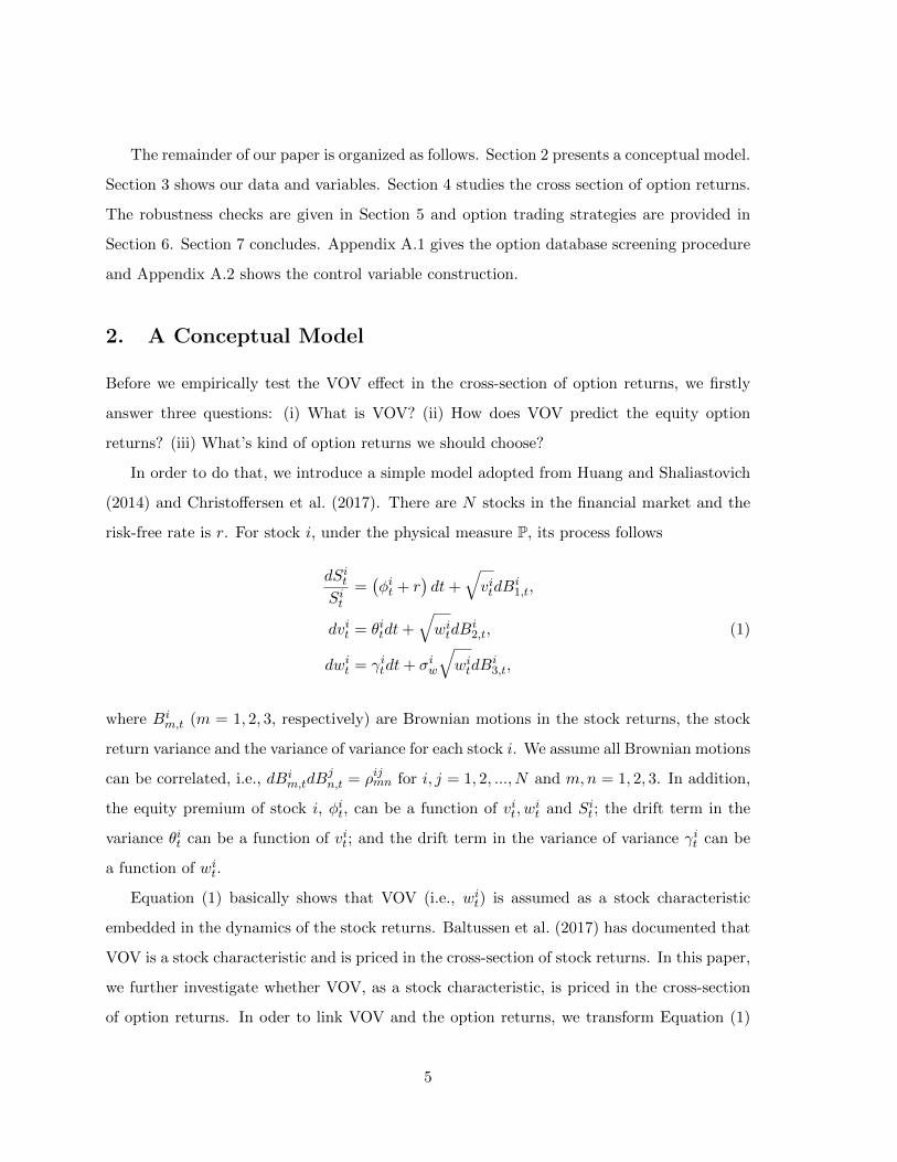
In order to do that, we introduce a simple model adopted from Huang and Shaliastovich

(2014) and Christoffersen et al. (2017). There are N stocks in the financial market and the

risk-free rate is r. For stock i, under the physical measure P, its process follows

dSitSit

=(φit + r

)dt+

√vitdB

i1,t,

dvit = θitdt+√witdB

i2,t, (1)

dwit = γitdt+ σiw

√witdB

i3,t,

where Bim,t (m = 1, 2, 3, respectively) are Brownian motions in the stock returns, the stock

return variance and the variance of variance for each stock i. We assume all Brownian motions

can be correlated, i.e., dBim,tdB

jn,t = ρijmn for i, j = 1, 2, ..., N and m,n = 1, 2, 3. In addition,

the equity premium of stock i, φit, can be a function of vit, wit and Sit ; the drift term in the

variance θit can be a function of vit; and the drift term in the variance of variance γit can be

a function of wit.

Equation (1) basically shows that VOV (i.e., wit) is assumed as a stock characteristic

embedded in the dynamics of the stock returns. Baltussen et al. (2017) has documented that

VOV is a stock characteristic and is priced in the cross-section of stock returns. In this paper,

we further investigate whether VOV, as a stock characteristic, is priced in the cross-section

of option returns. In oder to link VOV and the option returns, we transform Equation (1)

5

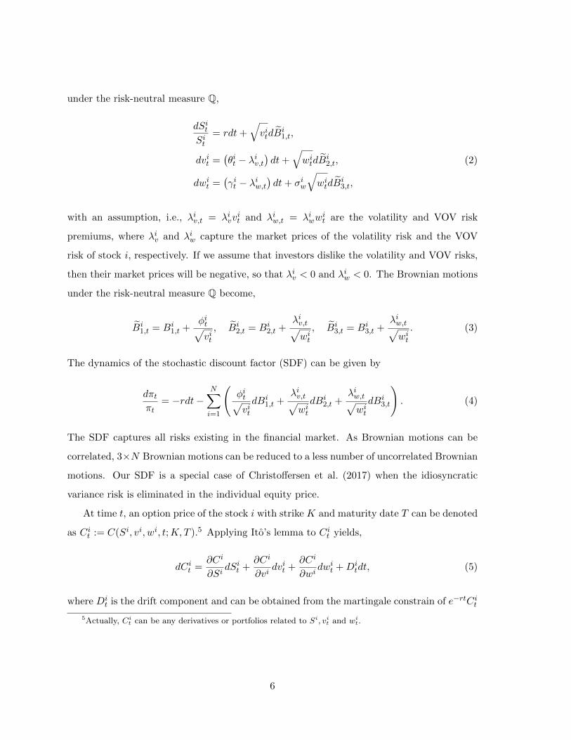
under the risk-neutral measure Q,

dSitSit

= rdt+√vitdB

i1,t,

dvit =(θit − λiv,t

)dt+

√witdB

i2,t, (2)

dwit =(γit − λiw,t

)dt+ σiw

√witdB

i3,t,

with an assumption, i.e., λiv,t = λivvit and λiw,t = λiww

it are the volatility and VOV risk

premiums, where λiv and λiw capture the market prices of the volatility risk and the VOV

risk of stock i, respectively. If we assume that investors dislike the volatility and VOV risks,

then their market prices will be negative, so that λiv < 0 and λiw < 0. The Brownian motions

under the risk-neutral measure Q become,

Bi1,t = Bi

1,t +φit√vit, Bi

2,t = Bi2,t +

λiv,t√wit, Bi

3,t = Bi3,t +

λiw,t√wit. (3)

The dynamics of the stochastic discount factor (SDF) can be given by

dπtπt

= −rdt−N∑i=1

(φit√vitdBi

1,t +λiv,t√witdBi

2,t +λiw,t√witdBi

3,t

). (4)

The SDF captures all risks existing in the financial market. As Brownian motions can be

correlated, 3×N Brownian motions can be reduced to a less number of uncorrelated Brownian

motions. Our SDF is a special case of Christoffersen et al. (2017) when the idiosyncratic

variance risk is eliminated in the individual equity price.

At time t, an option price of the stock i with strike K and maturity date T can be denoted

as Cit := C(Si, vi, wi, t;K,T ).5 Applying Ito’s lemma to Cit yields,

dCit =∂Ci

∂SidSit +

∂Ci

∂vidvit +

∂Ci

∂widwit +Di

tdt, (5)

where Dit is the drift component and can be obtained from the martingale constrain of e−rtCit

5Actually, Cit can be any derivatives or portfolios related to Si, vit and wit.

6

under the risk-neutral measure Q, i.e.,

∂Ci

∂SiSitr +

∂Ci

∂vi(θit − λiv,t

)+∂Ci

∂wi(γit − λiw,t

)+Di

t − rCit = 0. (6)

After solving the the drift component Dit from Equation (6),

Dit = r

(Cit −

∂Ci

∂SiSit

)− ∂Ci

∂vi(θit − λiv,t

)− ∂Ci

∂wi(γit − λiw,t

), (7)

we get the future option price Cit+τ from Equation (5), i.e.,

Cit+τ =Cit +

∫ t+τ

t

∂Ci

∂SidSiu +

∫ t+τ

t

∂Ci

∂vidviu +

∫ t+τ

t

∂Ci

∂widwiu

+

∫ t+τ

tr

(Cit −

∂Ci

∂SiSiu

)du−

∫ t+τ

t

∂Ci

∂vi(θiu − λiv,u

)du−

∫ t+τ

t

∂Ci

∂wi(γiu − λiw,u

)du.

(8)

Following Bakshi and Kapadia (2003), the delta-hedged option gain can be defined as

Πit,t+τ ≡ Cit+τ − Cit −

∫ t+τ

t

∂Ci

∂SidSiu −

∫ t+τ

tr

(Ciu −

∂Ci

∂SiSiu

)du. (9)

Plugging (8) and (1) into (9), we get

Πit,t+τ =

∫ t+τ

t

∂Ci

∂viλiv,udu+

∫ t+τ

t

∂Ci

∂wiλiw,udu+

∫ t+τ

t

∂Ci

∂vi

√wiudB

i2,u+

∫ t+τ

t

∂Ci

∂wiσw

√wiudB

i3,u.

(10)

The expected delta-hedged gain therefore can be solved as6

Et[Πit,t+τ ] = Et

(∫ t+τ

t

∂Ci

∂viλiv,udu

)+ Et

(∫ t+τ

t

∂Ci

∂wiλiw,udu

). (11)

Using the assumption, λiv,t = λivvit and λiw,t = λiww

it, according to Bakshi and Kapadia (2003)

6The expect gain of holding an option is simply given by

Et

[Cit+τ − Cit −

∫ t+τ

t

rCiudu

]= Et

(∫ t+τ

t

∂Ci

∂Siφiudu

)+Et

(∫ t+τ

t

∂Ci

∂viλiv,udu

)+Et

(∫ t+τ

t

∂Ci

∂wiλiw,udu

).

Without being delta-hedged, the expect gain of holding an option is also contributed by the equity premiumfrom the underlying stocks. In order to eliminate the impact from the equity premium, we consider thedelta-hedged gain throughout this paper.

7

and Huang and Shaliastovich (2014), Equation (11) can be expressed by

Et[Πit,t+τ ]

Sit= λivβ

iv,tv

it + λiwβ

iw,tw

it, (12)

where βiv,t > 0 and βiw,t > 0 are the sensitivities to the volatility and VOV risks, respectively.7

The denominator Sit is due that Cit ,∂Ci

∂viand ∂Ci

∂wiare homogeneous of degree 1 in Sit .

Equation (12) gives the relation between the expected delta-hedged gain, scaled by the

stock price, and the volatility and VOV risks. It reveals several important intuitions. (i)

the VOV effect is driven by the market price of the VOV risk. If investors dislike the VOV

risks, the VOV effect will be negative, i.e., the higher the VOV, the lower the expected

option returns. Equation (12) indeed provides an intuitive risk-based explanation for the

VOV effect. (ii) As the volatility effect is simultaneously modelled by Equation (12), it also

provides an alternative risk-based explanation for the results in Cao and Han (2013), i.e.,

the volatility effect is negative. Furthermore, the realized-implied volatility spread (RV-IV)

is a proxy of the variance risk premium λiv,t = λivvit = 1

dt

(E[dvit]− EQ[dvit]

). Equation (12)

therefore additionally explains the positive RV-IV effect, documented by Goyal and Saretto

(2009). (iii) The expected delta-hedged gain scaled by the initial stock price eliminates the

stock movements, so that it is a function of only the volatility and VOV risks. Taking this

advantage, the literature of the cross-section of the option returns mainly focuses on the

delta-hedged option returns, e.g., Goyal and Saretto (2009); Cao and Han (2013) and Cao

et al. (2017). (iv) As Cit can be a portfolio, any delta-hedged or delta-neutral option portfolios

should satisfy Equation (12), for example, the delta-neutral straddles studied by Goyal and

Saretto (2009); Cremers, Halling, and Weinbaum (2015) and Vasquez (2017).

Based on the above conceptual model, we know that VOV is a stock characteristic, similar

to the volatility of stock returns. VOV can negatively predict the future option returns (i.e.,

delta-hedged gains scaled by the underlying stock prices), if investors dislike the VOV risk.

In the following sections, we shall test the hypothesis that whether there is a negative relation

between the cross section of option returns and VOV.

7The sign of βiv,t (βiw,t) is determined by ∂Ci

∂v> 0 ( ∂C

i

∂wi > 0).

8

3. Data and Variables

3.1 Option data

Option data are obtained from the Ivy DB database provided by OptionMetrics, from 04

January 1996 to 29 April 2016. The data include daily closing bid and ask prices, trading

volume, option interest, implied volatility, delta and vega. Closing option prices are calculated

as the midpoint of the closing bid and ask prices. The monthly stock prices are obtained from

CRSP. Following Goyal and Saretto (2009); Cao and Han (2013); Boyer and Vorkink (2014)

and Byun and Kim (2016), firstly, we keep option data at the end of each month and merge

them with the CRSP data, keeping the sample if the closing price for the underlying stock

from CRSP is below 97% or above 103% of the closing price of the underlying stock from

the OptionMetrics database. Then we filter the option data based on Appendix A.1. After

that, we filter out options whose stocks have ex-dividend dates prior to option expiration

and eliminate options with moneyness (S/K) lower than 0.975 or higher than 1.025.8 At

the end of each month, we collect a pair of options that are closest to being at-the-money

(ATM) and have the shortest maturity among those with more than one month to expiration.

Following Cao and Han (2013), the maturity of the options we then pick each month has the

same maturity. We therefore drop the options whose maturity is different from that of the

maturity. Finally, we have 88,336 observations for both calls and puts. Our sample totally

considers 5,069 stocks and around 396 stocks per month.

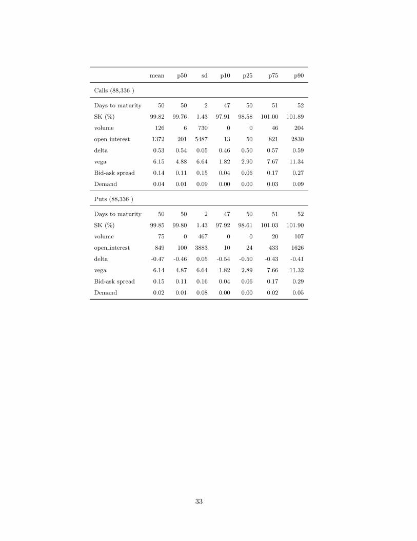
Panel A, Table 1 shows that the average moneyness of the chosen option is almost one,

with a standard deviation of only 0.01. The average delta of call options is close to 0.5 and

the average delta of put options is close to −0.5. In line with Cao and Han (2013), the time

to maturity of the chosen options ranges from 47 to 52 calendar days across different months,

with an average of 50 days. On average, the open interest and the trading volume of calls

are greater than puts. These short-term options are the most actively traded. Following Cao

and Han (2013), we calculate the bid-ask spread as the ratio of the difference between ask

8In line with Cao and Han (2013) and Cao et al. (2017), we alternatively keep options with moneyness(S/K) between 0.8 and 1.2. Using this filter, we obtain 224,504 observations for both calls and puts. Theaverage call option return is −0.29% with the median of −0.37% and the standard deviation of 3.18%. Theresults are given in Table IA.8–IA.10 in Internet Appendix and the VOV effect is even much stronger in thisscenario.

9

and bid quotes of options over the midpoint of bid and ask quotes at the end of each month,

and measure demand by the option open interest at the end of each month scaled by monthly

stock trading volume, i.e., (option open interest/stock volume)×103. The average bid-ask

spreads of call and put options are same, around 0.14. Because of greater open interest, the

demand of call options is higher than the demand of put options.

[Insert Table 1]

3.2 Option Returns

The delta-hedged gain defined in Equation (9) is from the continuous trading. In the reality,

the hedge should be rebalanced discretely. Consider a portfolio of an option (e.g., call option)

that is hedged discretely N times over a period [t, t+τ ] where the hedge is rebalanced at each

of the dates ti, i = 0, 1, ..., N −1 (where we define t0 = t and tN = t+ τ). In line with Bakshi

and Kapadia (2003) and Cao and Han (2013), we define the daily rebalanced delta-hedged

gain as follows.

Πit,t+τ = Cit+τ − Cit −

N−1∑i=0

∆iC,tn

(Sitn+1

− Sitn)−N−1∑i=0

rtnτtn(Citn −∆i

C,tnSitn

), (13)

where ∆iC,tn

is the delta of the option Ci at date tn; rtn is the annualized risk-free rate at

date tn and τtn is the number of calendar days between tn and tn+1 scaled by 365. The daily

risk-free rate is obtained from the Kenneth R. French Data Library.

Obviously, the initial investment in the delta-hedged option portfolio is zero, i.e., Πit,t = 0,

so that Πit,t+τ is the dollar return of the option portfolio. As Πi

t,t+τ is homogeneous of degree

1 in Sit , we scale the dollar return Πit,t+τ by the stock price Sit . Therefore, consistent with

Equation (12), the return of the option on stock i can be defined as

rit,t+τ =Πit,t+τ

Sit. (14)

At the end of each month, we construct one option portfolio and hold it until maturity

(which is on average 50 calendar days).9 Then the option return is the daily rebalanced

9We also run the cross-sectional regressions of option returns held until the end of month. The average

10

delta-hedged gain scaled by the initial stock price.10 We repeat this procedure each month

during the sample period and then we get a time series of option returns for each equity. In

the main content, we force on the call option returns defined in Equation (14) and provide

the results of the alternative returns in the robustness checks. From Panel B in Table 1, we

find that the average call option return is −0.26% with the standard deviation of 2.91%. The

median is higher than the mean, that is −0.49%.

3.3 VOV measure

Following Baltussen et al. (2017), we define the implied volatility (IV) as the average of the

ATM call and put implied volatilities, using the volatility surface standardized options with a

delta of 0.50 and maturity of 30 days. These data are obtained from Ivy DB OptionMetrics.

For each month t, the unscaled VOV is defined as the standard deviation of the ATM 30-day

IV, that is

V OV un,it = sd(IV i

d ), (15)

where IV id is the daily IV on day d of month t for stock i.

For a random variable iv (i.e., IV), we have sd(A×iv) = A×sd(iv) where A is a constant.

This indicates that the volatility of IV tends to be larger for the IV with larger magnitude.

In order to filter the volatility level effect from VOV, in line with Baltussen et al. (2017), we

scale V OV un,it by the mean of IV , i.e.,11

V OV it =

sd(IV id )

mean(IV id ). (16)

We require that there be at least 13 no-missing observations to calculate VOV. As IV is

the implied volatility, VOV is forward-looking. According to Baltussen et al. (2017), VOV

captures the uncertainty in investors’ assessment of the risks that surround future stock prices.

Epstein and Ji (2014) formulate a model to explain how investors’ ambiguity on volatility

call option return is −0.15% with the median of −0.37% and the standard deviation of 2.19%. The resultsare given in Tables IA.11–IA.13 in Internet Appendix and they are qualitatively same.

10In OptionMetrics, delta is missing in somedays. Therefore, we only rebalance the portfolio if delta is notmissing on that day, otherwise we hold it until the day has a non-missing delta.

11Using the unscaled VOV does not change our conclusion. See Table IA.2 in Internet Appendix. Expect-edly, for monthly Fama and MacBeth (1973) cross-sectional regressions, the magnitude and the significanceof the average VOV coefficient decrease a little after controlling IVOL or IV.

11

affects the asset prices. VOV does capture ambiguous volatility. Huang and Shaliastovich

(2014); Park (2015); Hollstein and Prokopczuk (2017) and our conceptual model show that

investors, who care uncertainty about volatility, are willing to pay a positive premium. The

negative market price of the VOV risk leads to the negative VOV effect.

Column (2), Panel C, Table 1 shows that for each year, the median of VOV across different

stocks is around 5 − 8%. Across different years, the medians of VOV are slightly different.

For example, in 2008, VOV reaches the maximal median of 8.35 during the sample period we

use. The unscaled VOV, reported in Column 1, Panel C, Table 1, varies a similar pattern of

VOV.

3.4 Control variables

The daily and monthly stock returns, stock prices, trading volume and share outstanding are

obtained from CRSP, and accounting and balance sheet data are obtained from COMPUS-

TAT, for calculating other control variables: the market beta (BETA), the log market capi-

talization (SIZE), the book-to-market ratio (BM), the return in the past month (REV), the

cumulative return from month t− 12 to month t− 2 (MOM), the log illiquidity (LN ILLIQ),

the maximum daily return (MAX) over the current month t, the idiosyncratic volatility

(IVOL), the realized skewness (RS) and the realized kurtosis (RK) based on daily returns

over the most recent 12 months.

By using volatility surface data provided by Ivy DB OptionMetrics, we are able to cal-

culate the model-free implied volatility (IV), the implied skewness (IS), the implied kurtosis

(IK), the volatility term structures (VTS) and the implied volatility innovations (dCIV and

dPIV). Finally, following Goyal and Saretto (2009), we calculate the realized-implied volatility

spread (RV IV) by using daily stock returns obtained from CRSP and the implied volatility

obtained from Ivy DB OptionMetrics. The details of control variable construction are pro-

vided in Appendix A.2. Following Cao and Han (2013) and Cao et al. (2017), we winsorize

all independent variables each month at the 0.5% level in order to eliminate the outliers. The

risk factors, including Fama and French (1993) three factors (MKT, SMB, HML), Carhart

(1997) momentum factor (UMD) and Fama and French (2015) five factors (RMW, CMA),

are obtained from the Kenneth R. French Data Library.

12

Panel D, Table 1 gives the summary statistics, which are close to the existing literature,

e.g., Cao and Han (2013); Byun and Kim (2016); Cao and Han (2013) and Baltussen et al.

(2017). Their correlations are given in Panel E, Table 1. The unscaled VOV, as a volatility-

related variable, is correlated to IVOL and IV, with a same correlation of 0.55. As VOV is

scaled by the average IV, VOV is almost independent of IV, with a correlation of 0.02. The

correlation between VOV and IVOL also reduces to 0.14. In addition, we find that there is

a high correlation between SIZE and LN ILLIQ, at a value of −0.91. It is intuitive, as the

small size stocks normally have high illiquidity.

4. Empirical results

In this section, we test the hypothesis of whether there is a negative relation between the

cross section of option returns and VOV, based on the monthly Fama and MacBeth (1973)

cross-sectional regressions,12 after controlling for existing popular determinants. The depen-

dent variable is the future option return, defined in (14), and the independent variables are

predetermined at the end of month t.

4.1 Univariate regression

As a benchmark, we present the univariate regression on VOV in the first column of Table

2, which shows that the delta-hedged call option returns are negatively related to the VOV,

without any control variables. The average coefficient of VOV is −0.018, with a significant

Newey and West (1987) t-statistic of −4.20. This confirms that VOV can negatively predict

the future option returns. This negative prediction further documents that the market price

of the VOV risk is negative and investors indeed dislike the VOV risk. Our empirical result

is therefore consistent with the intuition behind the conceptual model given in Section 2.

[Insert Table 2]

12Fama and MacBeth (1973) cross-sectional regressions are widely used to test the relation between thecross section of returns and the individual security variables, e.g., Brennan, Chordia, and Subrahmanyam(1998); Bali, Cakici, and Whitelaw (2011); Cao and Han (2013); Vasquez (2017) and others.

13

4.2 Controlling for firm-specific characteristics

All options are written on the underlying stocks. Straightforwardly, the underlying stock

characteristics may affect the relation between the option returns and VOV. Cao et al. (2017)

find that the delta-hedged equity option returns can be predicted by a variety of firm-specific

characteristics. Panel A, Table 2 reports the regression results after controlling for firm-

specific characteristics, i.e., the market beta (BETA), the log market capitalization (SIZE),

the book-to-market ratio (BM), the return in the past month (REV) and the cumulative

return from month t− 12 to month t− 2 (MOM).

The average coefficient of VOV remains negative and highly significant in all regressions

in Panel A, Table 2. All firm-specific characteristics does not materially affect the magnitude

and statistical significance of the VOV coefficient. The average VOV coefficient varies from

−0.018 to −0.020 and the Newey and West (1987) t-statistic ranges from −3.98 to −4.75.

This shows that the VOV effect cannot be explained by the firm-specific characteristics. The

result is expected, due to that VOV is almost independent of all firm-specific characteristics,

based on the correlations given in Panel E, Table 1.

4.3 Controlling for return distribution characteristics

According to Cao and Han (2013), the idiosyncratic volatility (IVOL) as a proxy of arbitrage

costs, is significantly and negatively related to the option returns. The higher premium

investors have to pay is due to the arbitrage costs. Model 2 in Panel B, Table 2 shows

that the IVOL coefficient is negative but not significant. Comparing Model 1 and Model 2

in Panel B, we find the VOV coefficient slightly decreases. The inconsistency between our

result and Cao and Han’s (2013) finding may be form the different data filters. Tables IA.8

in Internet Appendix gives further checks with an alternative data filter and shows that the

average coefficient of IVOL will be significant if we use the same data filter of moneyness

in Cao and Han (2013), i.e., keeping options with moneyness between 0.8 and 1.2. Using

a thinner moneyness range may generate deeper ATM options, so that the arbitrage costs

become lower due to the higher liquidity. Across different data filters, the VOV effect remains

negative and significant.

14

Byun and Kim (2016) suggest that call options written on the lottery-like stocks under-

perform. We control for the lottery demand factor, MAX, and find the VOV coefficient is not

affected. Furthermore, the average MAX coefficient is insignificant with a t-statistic of 0.069.

We could not find Byun and Kim’s (2016) observation in daily rebalanced delta-hedged call

option returns.

Based on the existing option pricing models ( e.g., Pan (2002) and Carr and Wu (2004)),

the jumps are the key factors for the option prices. We therefore control for the realized

skewness (RS) and the realized kurtosis (RK). Based on Model 4 and Model 5, we indeed

find a negative and significant relation between the option returns and jumps. The average

coefficient of RS in Model 4 is −0.00055 with a Newey and West (1987) t-statistic of −3.96 and

the average coefficient of RK in Model 5 is −0.00013 with a Newey and West (1987) t-statistic

of −5.32. RS and RK seem to have some predictive power for the option returns. Among

these return distribution characteristics, RK decreases the magnitude and the significance of

the VOV coefficient most. The average VOV coefficient reduces to −0.015 with a t-statistic

of −3.21 after controlling for RK. This indicates that VOV may have some jump information.

Even that, the negative VOV effect remains significant.

4.4 Controlling for limits to arbitrage

Cao and Han (2013) provide some evidence that the highly negative delta-hedge premium is

related to limits to arbitrage. Cao and Han (2013) consider three variables as proxies of limits

to arbitrage, i.e., the option demand (DEMAND), the option bid-ask spread (BID ASK)

which is a proxy of the option illiquidity and the log stock illiquidity (LN ILLIQ). Proxies of

limits to arbitrage essentially capture the option demand pressure and the illiquidity. From

Model 6 in Panel B, Table 2, we observe that the higher the option demand (DEMAND),

the lower the expected option returns. This is in line with the demand-based option pricing

theory in Garleanu, Pedersen, and Poteshman (2009). Furthermore, Model 4 in Panel B,

Table 2 shows that the higher the stock illiquidity (LN ILLIQ), the lower the expected option

returns. This is consistent with Kanne et al. (2016) and Christoffersen et al. (2018) who

provide evidence of a strong effect of the underlying stock’s illiquidity on option prices. After

controlling for all limits-to-arbitrage variables, the average VOV coefficient even increases.

15

Therefore, the VOV effect does come from limits to arbitrage.

4.5 Controlling for option-based characteristics

Hu and Jacobs (2017) find a negative relation between expected call option returns and the

volatility of stock returns. In this paper, we use the implied volatility (IV) as a proxy of the

volatility. Bali and Murray (2013) further suggest that the implied skewness (IS) can predict

the future returns of skewness assets.13 Goyal and Saretto (2009) find that the realized-

implied volatility spread (RV IV) can produce an economically and statistically significant

average monthly option return. Recently, Vasquez (2017) has found that the slope of the

implied volatility term structure (VTS) is positively related to future option returns. In

order to separate the VOV effect from these existing predictors, we control these predictors

in the regressions.

Furthermore, An, Ang, Bali, Cakici, et al. (2014) find that the implied volatility innova-

tions (dCIV and dPIV) can predict the future stock returns. The increase or decrease of the

forward-looking implied volatility, which represents the investors’ expectation of the market

moving direction in the future, may have some predictive power for the future option re-

turns. Due to that, we are also interested in investigating the effects of the implied volatility

innovations on the future option returns. All results are given in Panel D, Table 2.

First, Model 2 shows the average IV coefficient is −0.010 with a t-statistic of −5.28.

The option returns are negatively related to the IV. This is consistent with Hu and Jacobs

(2017) and is also identical to our conceptual model. From Models 3, we indeed find the

strong predictive power from IS, which is in line with Bali and Murray (2013). The positive

and significant RV IV coefficient in Model 5 suggests that the higher the realized-implied

volatility spread (RV IV), the higher the option returns. This is the same as the finding in

Bakshi and Kapadia (2003); Goyal and Saretto (2009); Cao and Han (2013) and Cao et al.

(2017). The positive RV IV effect is very intuitive. Bakshi and Kapadia (2003) suggest that

13We also use the IS calculated by using Bakshi, Kapadia, and Madan (2003) method and give the resultsin Table IA.3 in Internet Appendix. Roughly speaking, two measures work similarly. As Bakshi et al. (2003)method is restricted to the availability of the data to calculate the implied moments, more than 60% of stockshave missing IS. This is why the average VOV coefficient in Column 1, Table IA.3 is less significant than thatin Column 1, Table 2. In this paper, we therefore consider the construction approach in Bali, Hu, and Murray(2016), so that we can get enough observations.

16

the returns of delta-hedged option portfolios can be a proxy of the variance risk premium

and the RV IV self is a proxy of the variance risk premium. Therefore, RV IV can positively

predict the future option returns. Our conceptual model also confirms this observation.

The most influential control variable is VTS. The average VTS coefficient is 0.032 with a

significant Newey and West (1987) t-statistic of 7.85, based on Model 6. Vasquez (2017)

finds a significant and positive relation between the VTS and the straddle returns. Our

results suggest that there is also a significant and positive relation between the VTS and

the delta-hedged option returns. Model 7 shows that the implied volatility innovation from

calls (dCIV) has a significant and negative coefficient, at a value of −0.022 with a t-statistic

of −4.36. This effect in the cross section of option returns is opposite to that in the cross

section of stock returns, documented in An et al. (2014). A positive increase in the implied

volatility leads to the more negative expected option returns. In other words, investors dislike

the increase in the implied volatility and they are willing to pay a premium to hold options

whose implied volatility tends to increase. Finally, based on all regressions in Panel D, we

find the strength of the negative relation between the option returns and VOV is not reduced,

after controlling for these option-based characteristics.

5. Robustness checks

In this section, we provide several robustness checks for our new finding along different option

returns and different VOV proxies.

5.1 Different option returns

5.1.1 Delta-hedged put option returns

The results in the previous section are based on the delta-hedged call option returns. We

additionally calculate delta-hedged put option returns and give the summary statistics in Row

2, Panel B, Table 1. The average put option return is −0.04% with the standard deviation

of 2.94%, which is much higher than the average call option return, while their medians are

very close (i.e., −0.49% for calls and −0.28% for puts) and their correlation (unreported) is

over 0.94.

17

Table 3 reports the average coefficients from monthly Fama and MacBeth (1973) cross-

sectional regressions of delta-hedged put option returns. The result are almost the same with

call option return’s results in Table 2. This indicates that the VOV effect remains for the

delta-hedged put option returns. There are two observations that are different with the call

option return’s: (i) The IVOL effect is stronger in Panel B, Table 3, compared with the call

option returns in Table 2. This is intuitive. The put options are less liquid than the call

option implied by Panel A, Table 1. The arbitrage costs (i.e., IVOL) of put options are more

expensive. (ii) The average IS coefficient becomes significantly positive. The higher the IS,

the higher the expect put option returns. Intuitively, for holding put options, investors do like

the downside jumps in the future, which will lead to a low underlying stock price. Therefore,

put options on stocks with big forward-looking downside jumps (i.e., high IS put options) are

expected to achieve high option returns.

[Insert Table 3]

5.1.2 Alternative scales

Goyal and Saretto (2009) directly use the delta-hedged gains as option returns. As a ro-

bustness test, we also consider these dollar returns. The statistics of dollar returns Πt,τ are

given in Row 1, Panel B, Table 1. The average dollar return is −7.32%. In other words,

the average loss of holding an delta-hedged option portfolio until maturity is $0.0732. We

provide the firm-level cross-sectional regression results of delta-hedged gains in Table 4, which

is consistent with the results of delta-hedged gains scaled by the initial stock price.

[Insert Table 4]

We further scale the delta-hedged gain by the call option price (Cit) following Bakshi and

Kapadia (2003), Πit,t+τ/C

it , and the absolute value of the securities involved (∆i

tSit − Cit)

following Cao and Han (2013) and Cao et al. (2017), Πit,t+τ/(∆

itSit − Cit). Row 1, Panel B,

Table 1 gives their summary statistics. For both types of option returns, the cross-sectional

regression results in Tables 5 and 6 are qualitatively same with the results in Table 2.

[Insert Table 5]

[Insert Table 6]

18

5.1.3 Monthly rebalanced option returns

Option and stock trading involves significant costs, and strategies that hold over a certain

period [t, t + τ ] incur these costs only at initiation. In line with Goyal and Saretto (2009)

and Cao et al. (2017), we consider the monthly rebalanced delta-hedged gains, which can be

defined as

ΠM,it,t+τ = Ct+τ −∆C

t St+τ −(Ct −∆C

t St))

(1 + rtτ), (17)

to calculate the option returns. Equation (17) is a special case of Equation (13) when N =

1, i.e., the option portfolio is only hedged at initiation. From Row 3, Panel B, Table 1,

we find that the monthly rebalanced option returns rt,t+τ = ΠMt,τ/St are close to the daily

rebalanced option returns in statistics. The average monthly rebalanced return is −0.18%,

which is slightly larger than the average daily rebalanced return, −0.26%. Their correlation

(unreported) is 0.62. Expectedly, the regression results given in Table 7 are qualitatively

same with the results given in Table 2.

[Insert Table 7]

5.1.4 Delta-neutral straddle returns

The relation between the expected delta-hedged gain and VOV in Equation (12) is applicable

for any delta-neutral option portfolios. Due to that, following Goyal and Saretto (2009), we

finally consider the dollar gains of delta-neutral straddles,

ΠS,it,t+τ = cit+τ + pit+τ −

(cit + pit

)(1 + rtτ), (18)

where cit and pit are ATM call and put options at date t, respectively and have same strike

price. As two options used to construct each straddle (i.e., simultaneously long a call and a

put) are ATM and the delta of ATM call is around 0.5 and the delta of ATM put is around

−0.5 according to Panel A, Table 1, these straddles are delta-neutral.14 Each portfolio is

constructed at initiation and held until maturity.

14If options are not ATM, a delta-neutral straddle can be constructed by long a call and long −∆ic,t/∆

ip,t

number of put, where ∆ic,t (∆i

p,t) is the delta of the call (put) option at time t.

19

Row 4, Panel B, Table 1 shows that the average straddle return (i.e., rt,t+τ = ΠSt,τ/St)

is −0.13% with the standard deviation of 11.99%. The correlation (unreported) between

the straddle returns and the daily rebalanced call option returns is 0.58, and the correlation

(unreported) between the straddle returns and the monthly rebalanced call option returns is

0.98. This indicates that the delta-neutral straddle returns and delta-hedged option returns

consistently capture the risk premiums in a similar pattern. Unsurprisingly, a same conclusion

is made in the cross section of straddle returns in Table 8.

[Insert Table 8]

5.2 Different VOV measures

5.2.1 Term structure of VOV

Vasquez (2017) investigates the information embedded in the implied volatility term structure

and finds that the slope of the implied volatility term structure is positively related to future

option returns. This inspires that the implied volatility term structure causes the VOV term

structure. We therefore consider the volatility of volatility (VOV6M), which is defined as the

standard deviation of the ATM 6-month IV6M scaled by its mean,

V OV 6M it =

sd(IV 6M id)

mean(IV 6M id), (19)

where IV6M is the average of the ATM call and put implied volatilities, using the volatility

surface standardized options with a delta of 0.50 and maturity of six months.

Column 3, Panel C, Table 1 reports the 10th percentile (p10), 50th percentile (p50) and

90th percentile (p90) of the VOV6M across different years. Overall, the 6-month VOV6M

is smaller than the 30-day VOV. This leads to the slope of the term structure of the VOV,

VOV6M−VOV, is negative. The average slope (unreported) is around −4%.15 Even that,

the VOV6M still varies in a similar pattern of VOV, across different years. Their correlation

(unreported) is 0.81. The Fama and MacBeth (1973) cross-sectional regression results are

15We do find some predictive power from the slope of the term structure of VOV, while its predictiondepends on whether we control either VOV or VOV6M. As this is not our focus, in this paper, we only studythe option return predictability by using VOV6M.

20

given in Table 9. We find that the significance of the VOV6M coefficient is larger than the

significance of the VOV coefficient. It seems that the volatility of longer-maturity volatility

has more predictive power. This is consistent with the intuition that the 6-month VOV6M

is more informative than the 30-day VOV, in terms of predicting the future option returns

(over on average 50 calendar days).

[Insert Table 9]

5.2.2 Alternative VOV proxies

Agarwal et al. (2017) gives an alternative way to define VOV, i.e., the difference between the

natural log of the maximum of IV and the natural log of the minimum of IV in month t,

V OV al,it = ln

(max(IV i

d ))− ln

(min(IV i

d )). (20)

The summary statistics of the alternative VOV are given in Column 4, Panel C, Table

1. Roughly speaking, the alternative VOV varies similar to VOV (in Column 2). Actually,

the correlation (unreported) between the alternative VOV and the VOV reaches 0.96. The

alternative VOV therefore captures almost the same information with VOV. As a result,

their predictive power is qualitatively same, documented by the Fama and MacBeth (1973)

cross-sectional regressions in Table 10.

[Insert Table 10]

6. Portfolio Formation and Trading Strategy

In this section, we study the relation between option returns and VOV by using the portfolio

sorting approach, in order to confirm the previous results based on Fama and MacBeth (1973)

cross-sectional regressions.

6.1 Univariate portfolios sorted on VOV

Firstly, at the end of each month, we rank the delta-hedged option portfolios into 5 deciles,

based on VOV, and then form the 5 portfolios and calculate the equal-weighted monthly

21

returns of those 5 portfolios, respectively. Table 11 reports the average returns of the 5 port-

folios, each of which consists of long positions in daily rebalanced delta-hedged call options,

ranked in a given decile by VOV. Table 11 also reports the difference in the average returns

of the low and the high VOV decile portfolios in the “High-Low” row.

[Insert Table 11]

Column 1, Table 11 shows that the average subsequent returns of the 5 portfolios range

from −0.24 to −0.40. More importantly, we find the first three portfolios have same average

return, −0.24. This indicates that the VOV effect is very persistent. The option portfolios

with high VOV will be repeated in the future. Following Bali et al. (2011), we run the firm-

level cross-sectional regression of VOV on lagged predictors. Table 12 reports the average

coefficients, Newey and West (1987) t-statistics and the R-square. The R-square of the

univariate regression of lagged VOV is 19.6%, which documents that VOV has the substantial

cross-sectional explanatory power. Option portfolios with high VOV tend to exhibit similar

features in the following month. Other predictors all have univariate R-square of less than

5%. The average high-low return spread is −0.16% with a Newey and West (1987) t-statistic

of −2.90 in Column 1, Table 11. In other words, a portfolio held until maturity that buys

the lowest decile ranked by VOV and sells the highest decile can earn 0.16%.16

[Insert Table 12]

We use common risk factor models, i.e., the CAPM model, the Fama and French (1993)

three-factor model, the Carhart (1997) four-factor model and the Fama and French (2015)

five-factor model, to explain the significant negative high-low return spread. The second to

last columns in Table 11 give the results and show that the high-low return spread on option

portfolios sorted on the VOV cannot be explained by common risk factor models.

6.2 Bivariate portfolios sorted on control variables and the VOV

In line with the studies in Section 4, we consider two-way sorts–one based on the existing

predictors and the second based on VOV. We first rank the delta-hedged option portfolios

16If we use the delta-hedged option portfolios held until the end of month to form 5 portfolios sorted onVOV, the average high-low return spread is −0.15% with a even more significant t-statistic of −4.32 in Column1, Table IA.12.

22

into 5 deciles, based on each control variable, and then sequentially rank each decile into

another 5 deciles, based on VOV. Finally, we calculate the equal-weighted returns for each

VOV decile across 5 control deciles. Table 13 reports the average returns of the 5 portfolios

after controlling for the existing predictors and the average high-row return spread.

[Insert Table 13]

Similar to the univariate sorting result, the VOV effect is still economically and statisti-

cally significant after controlling for 18 variables in Table 13. The all average high-low return

spreads vary the almost same value with the one-way sort (i.e., −0.16%). This indicates

that the VOV effect is not contributed by other existing predictors. Therefore, the portfolio

sorting approach confirms the conclusion based on Fama and MacBeth (1973) cross-sectional

regressions, i.e., the VOV effect is significant and negative in the option market.17

7. Conclusion

This paper provides a comprehensive study of the relation between the delta-hedged option

returns and the volatility-of-volatility (VOV). Based on Fama and MacBeth (1973) cross-

sectional regressions and the portfolio sorting, we find a negative relation between option

returns and VOV, which is economically and statistically significant. This new finding is

regarded as the main contribution in this paper and is robust after controlling for numerous

risk factors and existing predictors. The negative VOV effect survives any robustness checks.

Our new finding also shows that VOV as a stock characteristic is priced by investors, with

a negative market price of the VOV risk. Investors indeed dislike uncertainty about volatility

of individual stocks, so that they are willing to pay a high premium to hold options with

high VOV. In addition, the VOV effect further suggests that it is important and fruitful to

consider the VOV risk in option pricing models, e.g., Huang and Shaliastovich (2014).

17The returns based on two-way sorts after controlling for common risk factors are given in Tables IA.4–IA.7in Internet Appendix and they are similar with the raw returns in Table 13.

23

A. Appendix

A.1 Option database screening procedure

1. Underlying Asset Is an Index: Optionmetrics “index flag” (index flag) is nonzero.

2. AM Settlement: The option expires at the market open of the last trading day, rather

than the close. Optionmetrics “am settlement flag”(am set flag) is nonzero.

3. Nonstandard Settlement: Optionmetrics “special settlement flag” (ss flag) is nonzero.

4. Abnormal Price: The price is less than $1/8; the bid price is zero or missing or is higher

than the ask price; the price violates arbitrage bounds.

5. Abnormal Implied Volatility: Implied volatility is less than zero or missing;

6. Abnormal Delta: Delta is less than −1 or larger than +1.

7. Zero Open Interest: Open interest is zero or missing.

A.2 Control variable construction

A.2.1 Firm-specific characteristics

• BETA: We run the market model at the daily frequency in month t to obtain the

monthly beta of an individual stock,

ri,d − rf,d = αi + β1,iMKTd−1 + β2,iMKTd + β3,iMKTd+1 + εi,d, (21)

where ri,d is the return on stock i on day d, MKTd is the market excess return on day

d, and rf,d is the risk-free rate on day d. The sum of the estimated slop coefficients,

β1,i + β2,i + β3,i, is the energy market beta of stock i in month t.

• SIZE: Firm size is measured as the natural log of the market value of equity at the end

of the month for each stock.

• Book-to-Market Ratio (BM): We compute the book-to-market ratio in month t of a firm

using the market value of its equity at the end of December of the previous year and

24

the book value of common equity plus balance-sheet deferred taxes for the firm’s latest

fiscal year ending in the prior calendar year, according to Fama and French (1993) and

Davis, Fama, and French (2000).

• Short-Term Reversal (REV): Following Jegadeesh (1990) and Lehmann (1990), we de-

fine short-term reversal for each stock in month t as the return on the stock over the

previous month from t− 1 to t.

• Momentum (MOM): Following Jegadeesh and Titman (1993), the momentum variable

for each stock in month t is defined as the cumulative return from month t − 12 to

month t− 2.

A.2.2 Limits to arbitrage

• Option Bid-Ask Spread (BID-ASK): Option bid-ask spread is the ratio of the difference

between ask and bid quotes of option over the midpoint of bid and ask quotes at the

end of each month.

• Option Demand (DEMAND): Option demand is measured by option open interest at

the end of each month scaled by monthly stock trading volume, according to Cao and

Han (2013), i.e., (option open interest/stock volume)×103.

• Stock Illiquidity (ILLIQ): Following Amihud (2002), the illiquidity, for each stock in

month t is defined as the annual average of the ratio of the absolute daily stock return

to its dollar trading volume over month t,

ILLIQi,t = 1/Di,t

Di,t∑d=1

|Ri,d|/V OLDi,d × 106, (22)

where Ri,d is the return on stock i on day d; Dt is the number of trading days in month

t; and V OLDi,t is the monthly trading volume of stock i in dollars.

A.2.3 Return distribution characteristics

• Maximum (MAX): MAX is the maximum daily return within a month, according to

Bali et al. (2011).

25

• Idiosyncratic Volatility (IVOL): Following Ang, Hodrick, Xing, and Zhang (2006), we

run the market model at the daily frequency,

ri,d − rf,d = αi + βi,MKTMKTd + βi,SMBSMBd + βi,HMLHMLd + εi,d, (23)

where ri,d is the return on stock i on day d, MKTd is the market return on day d, and

rf,d is the risk-free rate on day d. Idiosyncratic volatility of each stock in month t is

defined as the standard deviation of daily residuals in month t, IV OLi,t = sd(εi,d).

• Realized Skewness (RS): Realized skewness of stock i in month t is defined as the

skewness of daily returns over the most recent 12 months.

• Realized Kurtosis (RK): Realized kurtosis of stock i in month t is defined as the kurtosis

of daily returns over most recent 12 months.

A.2.4 Option-based characteristics

• Implied Volatility (IV): Implied volatility is the average of the at-the-money (ATM)

call and put implied volatilities, using the volatility surface standardized options with

a delta of 0.50 and maturity of 30 days, IV = CIV50+PIV502 , on the last trading day of

each month.

• Implied Skewness (IS): Following Bali et al. (2016), the implied skewness is the difference

between the ATM call and put implied volatilities with a delta of 0.25 and maturity of

30 days, ISt,τ = CIV25 − PIV25, on the last trading day of each month.

• Implied Kurtosis (IK): Following Bali et al. (2016), the implied kurtosis is the difference

between the sum of the 30-day ATM call and put implied volatilities with a delta of 0.25

and a delta of 0.50, IKt,τ = (CIV25 + PIV25) − (CIV50 + PIV50), on the last trading

day of each month.

• Realized-Implied Volatility Spread (RV IV): Following Goyal and Saretto (2009), realized-

implied volatility spread is the difference between RV and IV, where the annualized

realized volatility (RV) of stock i in month t is defined as the square root of 252 times

the standard deviation of daily returns over month t, RVi,t = sd(Ri,d)×√

252.

26

• Implied Volatility Innovation. According to An et al. (2014), implied volatility inno-

vation of calls dCIVi,t = CIVi,t − CIVi,t−1 and implied volatility innovation of puts

dPIVi,t = PIVi,t − PIVi,t−1, where CIV and PIV are the ATM call and put implied

volatilities with a delta of 0.50 and maturity of 30 days, respectively.

• Volatility Term Structures (VTS): Following Vasquez (2017), V TS = IV 6M − IV ,

where IV 6M is the average of the ATM call and put implied volatilities, using the

volatility surface standardized options with a delta of 0.50 and maturity of six months.

VTS in this paper captures the slope of the implied volatility term structure between

one month and six months.

27

References

Agarwal, Vikas, Y Eser Arisoy, and Narayan Y Naik, 2017, Volatility of aggregate volatility

and hedge funds returns, Journal of Financial Economics 125, 491–510.

Amihud, Yakov, 2002, Illiquidity and stock returns: cross-section and time-series effects,

Journal of Financial Markets 5, 31–56.

An, Byeong-Je, Andrew Ang, Turan G Bali, Nusret Cakici, et al., 2014, The joint cross

section of stocks and options, Journal of Finance 69, 2279–2337.

Ang, Andrew, Robert J Hodrick, Yuhang Xing, and Xiaoyan Zhang, 2006, The cross-section

of volatility and expected returns, Journal of Finance 61, 259–299.

Bakshi, Gurdip, and Nikunj Kapadia, 2003, Delta-hedged gains and the negative market

volatility risk premium, Review of Financial Studies 16, 527–566.

Bakshi, Gurdip, Nikunj Kapadia, and Dilip Madan, 2003, Stock return characteristics, skew

laws, and the differential pricing of individual equity options, Review of Financial Studies

16, 101–143.

Bali, Turan G, Nusret Cakici, and Robert F Whitelaw, 2011, Maxing out: Stocks as lotteries

and the cross-section of expected returns, Journal of Financial Economics 99, 427–446.

Bali, Turan G, Jianfeng Hu, and Scott Murray, 2016, Option implied volatility, skewness,

and kurtosis and the cross-section of expected stock returns, Available at SSRN 2322945 .

Bali, Turan G, and Scott Murray, 2013, Does risk-neutral skewness predict the cross-section

of equity option portfolio returns? Journal of Financial and Quantitative Analysis 48,

1145–1171.

Baltussen, Guido, Sjoerd Van Bekkum, and Bart Van Der Grient, 2017, Unknown unknowns:

uncertainty about risk and stock returns, Journal of Financial and Quantitative Analysis,

forthcomings .

Boyer, Brian H, and Keith Vorkink, 2014, Stock options as lotteries, Journal of Finance 69,

1485–1527.

28

Brennan, Michael J, Tarun Chordia, and Avanidhar Subrahmanyam, 1998, Alternative fac-

tor specifications, security characteristics, and the cross-section of expected stock returns,

Journal of Financial Economics 49, 345–373.

Byun, Suk-Joon, and Da-Hea Kim, 2016, Gambling preference and individual equity option

returns, Journal of Financial Economics 122, 155–174.

Cao, Jie, and Bing Han, 2013, Cross section of option returns and idiosyncratic stock volatil-

ity, Journal of Financial Economics 108, 231–249.

Cao, Jie, Bing Han, Qing Tong, and Xintong Zhan, 2017, Option return predictability, Avail-

able at SSRN 2698267 .

Carhart, Mark M, 1997, On persistence in mutual fund performance, Journal of Finance 52,

57–82.

Carr, Peter, and Liuren Wu, 2004, Time-changed levy processes and option pricing, Journal

of Financial Economics 71, 113–141.

Christoffersen, Peter, Mathieu Fournier, and Kris Jacobs, 2017, The factor structure in equity

options, Review of Financial Studies 31, 595–637.

Christoffersen, Peter, Ruslan Goyenko, Kris Jacobs, and Mehdi Karoui, 2018, Illiquidity

premia in the equity options market, Review of Financial Studies 31, 811–851.

Cremers, Martijn, Michael Halling, and David Weinbaum, 2015, Aggregate jump and volatil-

ity risk in the cross-section of stock returns, Journal of Finance 70, 577–614.

Davis, James L, Eugene F Fama, and Kenneth R French, 2000, Characteristics, covariances,

and average returns: 1929 to 1997, Journal of Finance 55, 389–406.

Epstein, Larry G, and Shaolin Ji, 2014, Ambiguous volatility, possibility and utility in con-

tinuous time, Journal of Mathematical Economics 50, 269–282.

Fama, Eugene F, and Kenneth R French, 1993, Common risk factors in the returns on stocks

and bonds, Journal of Financial Economics 33, 3–56.

29

Fama, Eugene F, and Kenneth R French, 2015, A five-factor asset pricing model, Journal of

Financial Economics 116, 1–22.

Fama, Eugene F, and James D MacBeth, 1973, Risk, return, and equilibrium: Empirical

tests, Journal of Political Economy 81, 607–636.

Garleanu, Nicolae, Lasse Heje Pedersen, and Allen M Poteshman, 2009, Demand-based option

pricing, Review of Financial Studies 22, 4259–4299.

Goyal, Amit, and Alessio Saretto, 2009, Cross-section of option returns and volatility, Journal

of Financial Economics 94, 310–326.

Green, T Clifton, and Stephen Figlewski, 1999, Market risk and model risk for a financial

institution writing options, Journal of Finance 54, 1465–1499.

Hollstein, Fabian, and Marcel Prokopczuk, 2017, How aggregate volatility-of-volatility affects

stock returns, Review of Asset Pricing Studies, forthcoming .

Hu, Guanglian, and Kris Jacobs, 2017, Volatility and expected option returns, Available at

SSRN 2695569 .

Huang, Darien, and Ivan Shaliastovich, 2014, Volatility-of-volatility risk, Available at SSRN

2497759 .

Jegadeesh, Narasimhan, 1990, Evidence of predictable behavior of security returns, Journal

of Finance 45, 881–898.

Jegadeesh, Narasimhan, and Sheridan Titman, 1993, Returns to buying winners and selling

losers: Implications for stock market efficiency, Journal of Finance 48, 65–91.

Kanne, Stefan, Olaf Korn, and Marliese Uhrig-Homburg, 2016, Stock illiquidity, option prices,

and option returns, Available at SSRN 2699529 .

Lehmann, Bruce N, 1990, Fads, martingales, and market efficiency, Quarterly Journal of

Economics 105, 1–28.

Muravyev, Dmitriy, 2016, Order flow and expected option returns, Journal of Finance 71,

673–708.

30

Newey, Whitney K, and Kenneth D West, 1987, A simple, positive semi-definite, het-

eroskedasticity and autocorrelation consistent covariance matrix, Econometrica 55, 703–08.

Pan, Jun, 2002, The jump-risk premia implicit in options: Evidence from an integrated

time-series study, Journal of Financial Economics 63, 3–50.

Park, Yang-Ho, 2015, Volatility-of-volatility and tail risk hedging returns, Journal of Finan-

cial Markets 26, 38–63.

Vasquez, Aurelio, 2017, Equity volatility term structures and the cross-section of option

returns, Journal of Financial and Quantitative Analysis 52, 2727–2754.

31

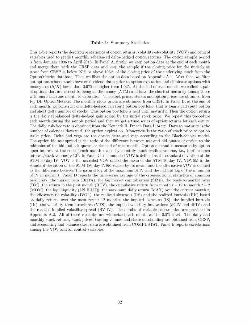
Table 1: Summary Statistics

This table reports the descriptive statistics of option returns, volatility-of-volatility (VOV) and controlvariables used to predict monthly rebalanced delta-hedged option returns. The option sample periodis from January 1996 to April 2016. In Panel A, firstly, we keep option data at the end of each monthand merge them with the CRSP data and keep the sample if the closing price for the underlyingstock from CRSP is below 97% or above 103% of the closing price of the underlying stock from theOptionMetrics database. Then we filter the option data based on Appendix A.1. After that, we filterout options whose stocks have ex-dividend dates prior to option expiration and eliminate options withmoneyness (S/K) lower than 0.975 or higher than 1.025. At the end of each month, we collect a pairof options that are closest to being at-the-money (ATM) and have the shortest maturity among thosewith more than one month to expiration. The stock prices, strikes and option prices are obtained fromIvy DB OptionMetrics. The monthly stock prices are obtained from CRSP. In Panel B, at the end ofeach month, we construct one delta-hedged call (put) option portfolio, that is long a call (put) optionand short delta number of stocks. This option portfolio is held until maturity. Then the option returnis the daily rebalanced delta-hedged gain scaled by the initial stock price. We repeat this procedureeach month during the sample period and then we get a time series of option returns for each equity.The daily risk-free rate is obtained from the Kenneth R. French Data Library. Days to maturity is thenumber of calendar days until the option expiration. Moneyness is the ratio of stock price to optionstrike price. Delta and vega are the option delta and vega according to the Black-Scholes model.The option bid-ask spread is the ratio of the difference between ask and bid quotes of option to themidpoint of the bid and ask quotes at the end of each month. Option demand is measured by optionopen interest at the end of each month scaled by monthly stock trading volume, i.e., (option openinterest/stock volume)×103. In Panel C, the unscaled VOV is defined as the standard deviation of theATM 30-day IV; VOV is the unscaled VOV scaled the mean of the ATM 30-day IV; VOV6M is thestandard deviation of the ATM 180-day IV6M scaled by its mean; and the alternative VOV is definedas the difference between the natural log of the maximum of IV and the natural log of the minimumof IV in month t. Panel D reports the time-series average of the cross-sectional statistics of commonpredictors: the market beta (BETA), the log market capitalization (SIZE), the book-to-market ratio(BM), the return in the past month (REV), the cumulative return from month t− 12 to month t− 2(MOM), the log illiquidity (LN ILLIQ), the maximum daily return (MAX) over the current month t,the idiosyncratic volatility (IVOL), the realized skewness (RS) and the realized kurtosis (RK) basedon daily returns over the most recent 12 months, the implied skewness (IS), the implied kurtosis(IK), the volatility term structures (VTS), the implied volatility innovations (dCIV and dPIV) andthe realized-implied volatility spread (RV IV). The details of variable construction are provided inAppendix A.2. All of these variables are winsorized each month at the 0.5% level. The daily andmonthly stock returns, stock prices, trading volume and share outstanding are obtained from CRSP,and accounting and balance sheet data are obtained from COMPUSTAT. Panel E reports correlationsamong the VOV and all control variables.

32

mean p50 sd p10 p25 p75 p90

Calls (88,336 )

Days to maturity 50 50 2 47 50 51 52

SK (%) 99.82 99.76 1.43 97.91 98.58 101.00 101.89

volume 126 6 730 0 0 46 204

open interest 1372 201 5487 13 50 821 2830

delta 0.53 0.54 0.05 0.46 0.50 0.57 0.59

vega 6.15 4.88 6.64 1.82 2.90 7.67 11.34

Bid-ask spread 0.14 0.11 0.15 0.04 0.06 0.17 0.27

Demand 0.04 0.01 0.09 0.00 0.00 0.03 0.09

Puts (88,336 )

Days to maturity 50 50 2 47 50 51 52

SK (%) 99.85 99.80 1.43 97.92 98.61 101.03 101.90

volume 75 0 467 0 0 20 107

open interest 849 100 3883 10 24 433 1626

delta -0.47 -0.46 0.05 -0.54 -0.50 -0.43 -0.41

vega 6.14 4.87 6.64 1.82 2.89 7.66 11.32

Bid-ask spread 0.15 0.11 0.16 0.04 0.06 0.17 0.29

Demand 0.02 0.01 0.08 0.00 0.00 0.02 0.05

33

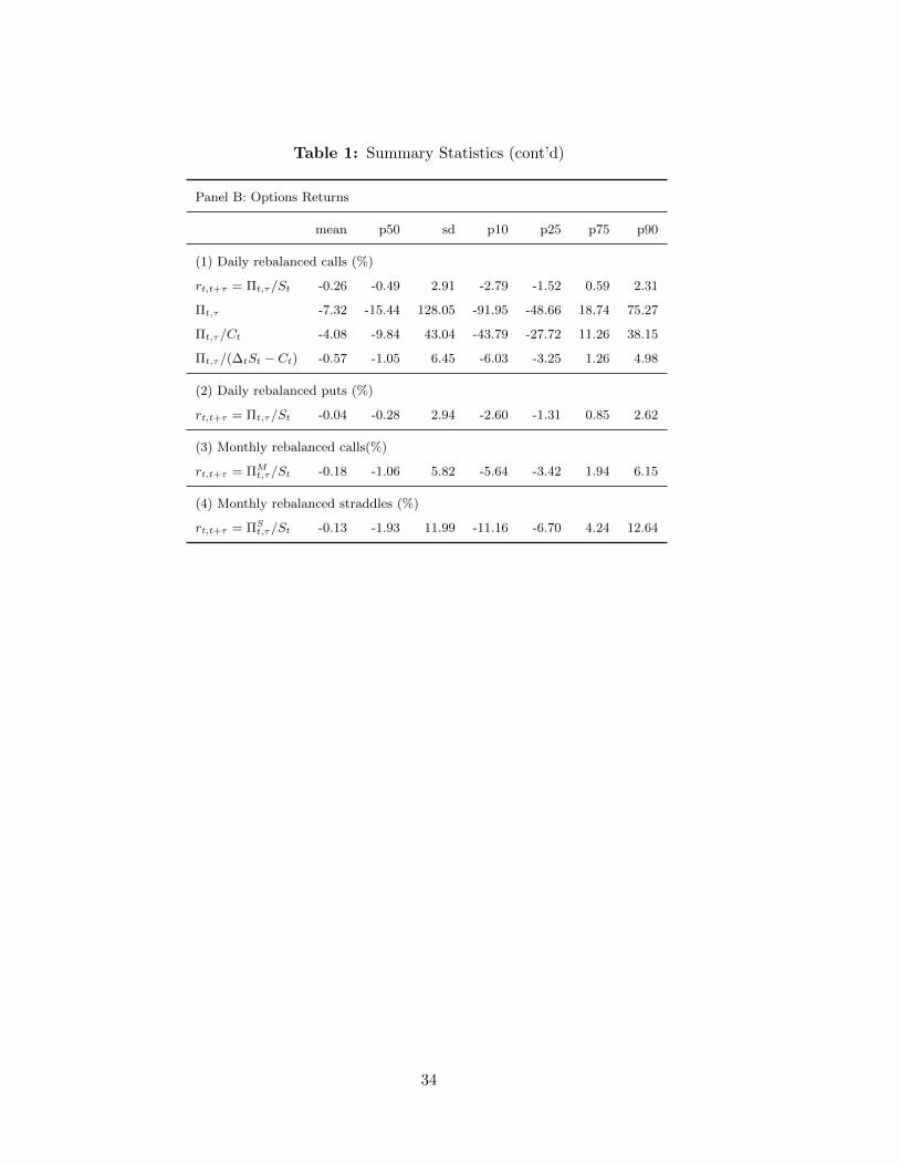
Table 1: Summary Statistics (cont’d)

Panel B: Options Returns

mean p50 sd p10 p25 p75 p90

(1) Daily rebalanced calls (%)

rt,t+τ = Πt,τ/St -0.26 -0.49 2.91 -2.79 -1.52 0.59 2.31

Πt,τ -7.32 -15.44 128.05 -91.95 -48.66 18.74 75.27

Πt,τ/Ct -4.08 -9.84 43.04 -43.79 -27.72 11.26 38.15

Πt,τ/(∆tSt − Ct) -0.57 -1.05 6.45 -6.03 -3.25 1.26 4.98

(2) Daily rebalanced puts (%)

rt,t+τ = Πt,τ/St -0.04 -0.28 2.94 -2.60 -1.31 0.85 2.62

(3) Monthly rebalanced calls(%)

rt,t+τ = ΠMt,τ/St -0.18 -1.06 5.82 -5.64 -3.42 1.94 6.15

(4) Monthly rebalanced straddles (%)

rt,t+τ = ΠSt,τ/St -0.13 -1.93 11.99 -11.16 -6.70 4.24 12.64

34

Table 1: Summary Statistics (cont’d)

Panel C: VOV

(1) VOVun (%) (2) VOV (%) (3) VOV6M (%) (4) VOVal(%)

Year p10 p50 p90 p10 p50 p90 p10 p50 p90 p10 p50 p90

1996 0.72 1.90 5.87 2.52 5.20 11.04 1.04 2.60 6.68 9.47 18.69 38.64

1997 0.73 1.99 5.79 2.31 5.05 11.17 0.96 2.49 6.84 8.65 18.42 37.23

1998 0.83 2.31 7.29 2.39 5.31 12.45 1.00 2.76 7.55 8.81 19.02 41.88

1999 0.88 2.41 7.52 2.01 4.72 10.98 0.87 2.45 7.13 7.47 16.76 36.39

2000 1.14 3.28 9.95 2.10 5.18 11.76 0.87 2.47 7.18 7.83 17.83 38.68

2001 1.08 2.93 8.44 2.46 5.84 12.86 1.16 2.94 7.57 8.87 19.92 40.02

2002 1.09 2.94 7.80 2.94 6.65 14.14 1.44 3.35 8.07 10.73 22.82 45.31

2003 0.95 2.24 5.38 3.22 6.38 11.88 1.45 3.00 6.47 11.89 22.21 39.09

2004 0.79 1.78 4.51 3.00 5.88 11.01 1.27 2.57 5.46 11.13 20.90 37.55

2005 0.73 1.72 4.66 2.98 6.03 12.60 1.21 2.57 5.79 11.00 21.41 43.05

2006 0.80 1.87 4.74 3.18 6.10 12.02 1.26 2.57 5.67 11.59 21.39 41.18

2007 0.95 2.14 5.23 3.60 6.71 13.28 1.63 3.33 7.33 13.01 23.79 45.78

2008 1.49 3.85 10.57 4.05 8.35 15.48 1.86 3.89 9.27 14.91 29.30 54.57

2009 1.44 3.01 6.31 3.75 6.60 11.45 1.81 3.30 6.05 13.86 23.56 38.58

2010 1.16 2.39 5.16 3.86 6.97 12.40 1.83 3.57 6.92 14.12 24.82 43.25

2011 1.21 2.69 6.71 4.13 7.55 14.64 1.89 3.75 8.50 15.15 27.58 53.45

2012 1.08 2.25 5.39 4.10 7.39 13.25 1.85 3.40 6.81 14.99 26.19 45.37

2013 0.88 1.84 4.90 3.53 6.64 13.83 1.42 2.79 5.51 13.11 23.74 46.35

2014 0.91 2.16 5.74 3.72 7.66 15.68 1.28 2.71 6.22 13.80 26.56 52.28

2015 1.04 2.30 6.28 3.97 7.54 16.14 1.64 3.10 6.70 14.40 27.18 54.52

2016 1.24 2.83 7.26 4.31 8.03 15.06 2.05 3.83 6.80 15.38 28.50 51.87

35

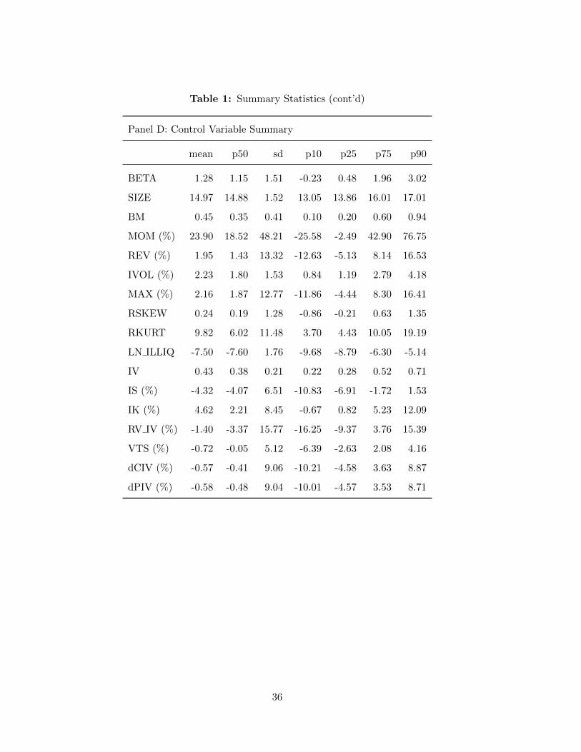
Table 1: Summary Statistics (cont’d)

Panel D: Control Variable Summary

mean p50 sd p10 p25 p75 p90

BETA 1.28 1.15 1.51 -0.23 0.48 1.96 3.02

SIZE 14.97 14.88 1.52 13.05 13.86 16.01 17.01

BM 0.45 0.35 0.41 0.10 0.20 0.60 0.94

MOM (%) 23.90 18.52 48.21 -25.58 -2.49 42.90 76.75

REV (%) 1.95 1.43 13.32 -12.63 -5.13 8.14 16.53

IVOL (%) 2.23 1.80 1.53 0.84 1.19 2.79 4.18

MAX (%) 2.16 1.87 12.77 -11.86 -4.44 8.30 16.41

RSKEW 0.24 0.19 1.28 -0.86 -0.21 0.63 1.35

RKURT 9.82 6.02 11.48 3.70 4.43 10.05 19.19

LN ILLIQ -7.50 -7.60 1.76 -9.68 -8.79 -6.30 -5.14

IV 0.43 0.38 0.21 0.22 0.28 0.52 0.71

IS (%) -4.32 -4.07 6.51 -10.83 -6.91 -1.72 1.53

IK (%) 4.62 2.21 8.45 -0.67 0.82 5.23 12.09

RV IV (%) -1.40 -3.37 15.77 -16.25 -9.37 3.76 15.39

VTS (%) -0.72 -0.05 5.12 -6.39 -2.63 2.08 4.16

dCIV (%) -0.57 -0.41 9.06 -10.21 -4.58 3.63 8.87

dPIV (%) -0.58 -0.48 9.04 -10.01 -4.57 3.53 8.71

36

Table 1: Summary Statistics (cont’d)

Panel E: Correlations

VOVun VOV VOV6M VOVal BETA SIZE BM MOM REV IVOL MAX RS

VOVun 1.00VOV 0.76 1.00VOV6M 0.59 0.70 1.00

VOVal 0.74 0.96 0.69 1.00BETA 0.13 0.00 0.00 0.00 1.00SIZE -0.26 -0.01 -0.03 -0.02 -0.10 1.00BM -0.02 0.01 0.06 0.02 0.00 -0.09 1.00MOM 0.05 -0.03 -0.04 -0.03 0.09 -0.02 -0.14 1.00REV -0.08 -0.07 -0.06 -0.07 0.00 0.01 0.02 -0.01 1.00IVOL 0.55 0.14 0.19 0.13 0.18 -0.39 -0.08 0.15 -0.04 1.00MAX 0.00 -0.01 0.00 -0.01 0.03 -0.07 0.02 -0.01 -0.02 0.10 1.00RS 0.08 0.06 0.07 0.06 0.02 -0.05 -0.03 0.27 0.10 0.09 0.11 1.00RK 0.15 0.16 0.13 0.17 -0.01 -0.16 -0.06 0.03 0.01 0.13 0.02 0.24DEMAND -0.03 -0.01 0.00 -0.01 -0.04 -0.10 0.01 -0.03 0.03 -0.06 0.06 0.04BID ASK 0.15 0.23 0.21 0.26 -0.04 -0.38 0.12 -0.07 -0.02 -0.01 -0.02 0.03IV 0.55 0.02 0.09 0.01 0.23 -0.47 -0.06 0.16 -0.02 0.76 -0.03 0.08IS -0.21 -0.08 -0.11 -0.08 -0.07 -0.01 -0.01 0.03 0.02 -0.13 -0.02 -0.03IK 0.14 0.21 0.17 0.23 -0.03 -0.25 0.10 -0.08 -0.03 0.00 -0.02 0.00RV IV 0.28 0.25 0.27 0.26 0.15 0.04 -0.01 0.01 -0.08 0.57 0.15 0.02VTS -0.29 -0.07 -0.15 -0.07 -0.06 0.10 0.02 -0.01 0.04 -0.32 0.12 -0.03dCIV -0.05 -0.07 -0.01 -0.07 0.00 0.06 -0.03 0.04 0.08 -0.01 -0.35 -0.02dPIV -0.03 -0.06 0.01 -0.05 0.01 0.06 -0.03 0.04 0.05 0.00 -0.30 -0.02

RK DEMAND BID ASK LN ILLIQ IV IS IK RV IV VTS dCIV dPIV

RK 1.00DEMAND 0.05 1.00BID ASK 0.08 0.02 1.00LN ILLIQ 0.09 0.11 0.41 1.00IV 0.06 -0.03 -0.02 0.49 1.00IS 0.01 0.02 0.09 0.02 -0.23 1.00IK 0.07 0.06 0.51 0.27 -0.04 0.13 1.00RV IV 0.05 -0.11 -0.03 -0.01 0.03 -0.06 0.02 1.00VTS -0.03 0.04 -0.02 -0.15 -0.52 0.17 0.09 0.07 1.00dCIV -0.01 -0.03 -0.06 -0.03 0.17 0.02 -0.11 -0.18 -0.50 1.00dPIV -0.01 -0.02 -0.04 -0.03 0.17 -0.12 -0.10 -0.16 -0.50 0.79 1.00

37

Table 2: Firm-level cross-sectional regressions of delta-hedged call option returns

This table reports the average coefficients from monthly Fama and MacBeth (1973) cross-sectionalregressions of delta-hedged call option returns. Volatility of volatility (VOV) is defined as the standarddeviation of the ATM 30-day IV scaled by its mean and the details of control variable constructionare provided in Appendix A.2. All independent variables are winsorized each month at the 0.5% level.The sample period is from January 1996 to April 2016. To adjust for serial correlation, robust Neweyand West (1987) t-statistics are reported in parentheses. *, ** and *** indicates significance at the10, 5 and 1% level.

Panel A: Firm-Specific Characteristics

(1) (2) (3) (4) (5) (6) (7)

VOV -0.018*** -0.020*** -0.018*** -0.019*** -0.019*** -0.018*** -0.020***(-4.20) (-4.75) (-4.15) (-4.23) (-4.43) (-3.98) (-4.57)

BETA 0.00041* 0.00026(1.88) (1.17)

SIZE 0.00062*** 0.00051***(3.68) (3.46)

BM -0.00075 -0.00032(-0.84) (-0.41)

MOM -0.00067 -0.00063(-1.28) (-1.32)

REV -0.00075 -0.00072(-0.43) (-0.41)

R-squared 0.009 0.018 0.019 0.016 0.020 0.018 0.051

Panel B: Return Distribution Characteristics

(1) (2) (3) (4) (5) (6)

VOV -0.018*** -0.016*** -0.021*** -0.018*** -0.015*** -0.016***(-4.20) (-3.99) (-5.11) (-3.95) (-3.21) (-4.03)

IVOL -0.035 -0.036*(-1.63) (-1.70)

MAX 0.00013 0.0020(0.069) (1.04)

RS -0.00055*** -0.00036***(-3.96) (-3.23)

RK -0.00013*** -0.00010***(-5.32) (-4.72)

R-squared 0.009 0.023 0.020 0.015 0.017 0.045

Panel C: Limits to Arbitrage

(1) (2) (3) (4) (5)

VOV -0.018*** -0.018*** -0.017*** -0.019*** -0.020***(-4.20) (-4.30) (-4.08) (-4.53) (-4.80)

DEMAND -0.019*** -0.017***(-4.29) (-3.02)

BID ASK -0.0036 0.0046(-1.13) (1.65)

LN ILLIQ -0.00065*** -0.00066***(-3.63) (-3.62)

R-squared 0.009 0.016 0.018 0.021 0.035

Panel D:Option-based Characteristics

(1) (2) (3) (4) (5) (6) (7) (8)

VOV -0.018*** -0.016*** -0.019*** -0.020*** -0.027*** -0.017*** -0.021*** -0.027***(-4.20) (-3.71) (-4.67) (-4.46) (-7.32) (-4.03) (-5.26) (-6.67)

IV -0.010*** -0.0094***(-5.28) (-5.13)

IS -0.017*** -0.020***(-4.53) (-5.84)

IK 0.0069** 0.0052*(2.13) (1.69)

RV IV 0.011*** 0.0089***(7.85) (5.22)

VTS 0.032*** 0.0096**(6.26) (1.97)

dCIV -0.019*** -0.012***(-7.73) (-4.19)

R-squared 0.009 0.036 0.020 0.016 0.021 0.025 0.022 0.083

38

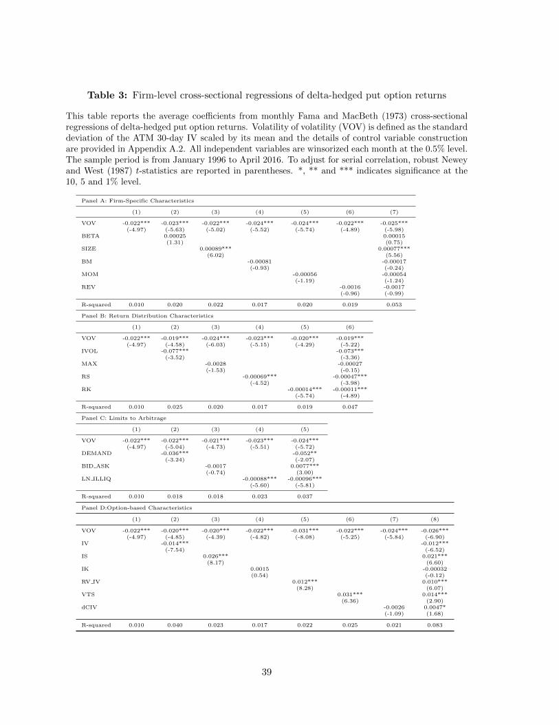
Table 3: Firm-level cross-sectional regressions of delta-hedged put option returns

This table reports the average coefficients from monthly Fama and MacBeth (1973) cross-sectionalregressions of delta-hedged put option returns. Volatility of volatility (VOV) is defined as the standarddeviation of the ATM 30-day IV scaled by its mean and the details of control variable constructionare provided in Appendix A.2. All independent variables are winsorized each month at the 0.5% level.The sample period is from January 1996 to April 2016. To adjust for serial correlation, robust Neweyand West (1987) t-statistics are reported in parentheses. *, ** and *** indicates significance at the10, 5 and 1% level.

Panel A: Firm-Specific Characteristics

(1) (2) (3) (4) (5) (6) (7)

VOV -0.022*** -0.023*** -0.022*** -0.024*** -0.024*** -0.022*** -0.025***(-4.97) (-5.63) (-5.02) (-5.52) (-5.74) (-4.89) (-5.98)

BETA 0.00025 0.00015(1.31) (0.75)

SIZE 0.00089*** 0.00077***(6.02) (5.56)

BM -0.00081 -0.00017(-0.93) (-0.24)

MOM -0.00056 -0.00054(-1.19) (-1.24)

REV -0.0016 -0.0017(-0.96) (-0.99)

R-squared 0.010 0.020 0.022 0.017 0.020 0.019 0.053

Panel B: Return Distribution Characteristics

(1) (2) (3) (4) (5) (6)

VOV -0.022*** -0.019*** -0.024*** -0.023*** -0.020*** -0.019***(-4.97) (-4.58) (-6.03) (-5.15) (-4.29) (-5.22)

IVOL -0.077*** -0.073***(-3.52) (-3.36)

MAX -0.0028 -0.00027(-1.53) (-0.15)

RS -0.00069*** -0.00047***(-4.52) (-3.98)

RK -0.00014*** -0.00011***(-5.74) (-4.89)

R-squared 0.010 0.025 0.020 0.017 0.019 0.047

Panel C: Limits to Arbitrage

(1) (2) (3) (4) (5)

VOV -0.022*** -0.022*** -0.021*** -0.023*** -0.024***(-4.97) (-5.04) (-4.73) (-5.51) (-5.72)

DEMAND -0.036*** -0.052**(-3.24) (-2.07)

BID ASK -0.0017 0.0077***(-0.74) (3.00)

LN ILLIQ -0.00088*** -0.00096***(-5.60) (-5.81)

R-squared 0.010 0.018 0.018 0.023 0.037

Panel D:Option-based Characteristics

(1) (2) (3) (4) (5) (6) (7) (8)

VOV -0.022*** -0.020*** -0.020*** -0.022*** -0.031*** -0.022*** -0.024*** -0.026***(-4.97) (-4.85) (-4.39) (-4.82) (-8.08) (-5.25) (-5.84) (-6.90)

IV -0.014*** -0.012***(-7.54) (-6.52)

IS 0.026*** 0.021***(8.17) (6.60)

IK 0.0015 -0.00032(0.54) (-0.12)

RV IV 0.012*** 0.010***(8.28) (6.07)

VTS 0.031*** 0.014***(6.36) (2.90)

dCIV -0.0026 0.0047*(-1.09) (1.68)

R-squared 0.010 0.040 0.023 0.017 0.022 0.025 0.021 0.083

39

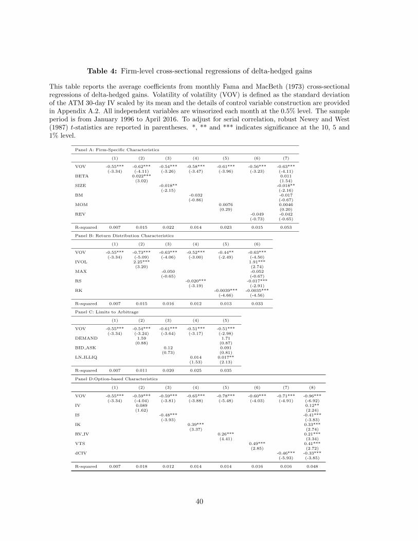
Table 4: Firm-level cross-sectional regressions of delta-hedged gains

This table reports the average coefficients from monthly Fama and MacBeth (1973) cross-sectionalregressions of delta-hedged gains. Volatility of volatility (VOV) is defined as the standard deviationof the ATM 30-day IV scaled by its mean and the details of control variable construction are providedin Appendix A.2. All independent variables are winsorized each month at the 0.5% level. The sampleperiod is from January 1996 to April 2016. To adjust for serial correlation, robust Newey and West(1987) t-statistics are reported in parentheses. *, ** and *** indicates significance at the 10, 5 and1% level.

Panel A: Firm-Specific Characteristics

(1) (2) (3) (4) (5) (6) (7)

VOV -0.55*** -0.62*** -0.54*** -0.58*** -0.61*** -0.56*** -0.63***(-3.34) (-4.11) (-3.26) (-3.47) (-3.96) (-3.23) (-4.11)

BETA 0.022*** 0.011(3.02) (1.54)

SIZE -0.018** -0.018**(-2.15) (-2.16)

BM -0.032 -0.017(-0.86) (-0.67)

MOM 0.0076 0.0046(0.29) (0.20)

REV -0.049 -0.042(-0.73) (-0.65)

R-squared 0.007 0.015 0.022 0.014 0.023 0.015 0.053

Panel B: Return Distribution Characteristics

(1) (2) (3) (4) (5) (6)

VOV -0.55*** -0.73*** -0.63*** -0.52*** -0.44** -0.63***(-3.34) (-5.09) (-4.06) (-3.00) (-2.49) (-4.50)

IVOL 2.25*** 1.91***(3.20) (2.74)

MAX -0.050 -0.052(-0.65) (-0.67)

RS -0.020*** -0.017***(-3.19) (-2.91)

RK -0.0039*** -0.0035***(-4.66) (-4.56)

R-squared 0.007 0.015 0.016 0.012 0.013 0.033

Panel C: Limits to Arbitrage

(1) (2) (3) (4) (5)

VOV -0.55*** -0.54*** -0.61*** -0.51*** -0.51***(-3.34) (-3.24) (-3.64) (-3.17) (-2.98)

DEMAND 1.59 1.71(0.88) (0.87)

BID ASK 0.12 0.091(0.73) (0.81)

LN ILLIQ 0.014 0.017**(1.53) (2.13)

R-squared 0.007 0.011 0.020 0.025 0.035

Panel D:Option-based Characteristics

(1) (2) (3) (4) (5) (6) (7) (8)

VOV -0.55*** -0.59*** -0.59*** -0.65*** -0.78*** -0.60*** -0.71*** -0.96***(-3.34) (-4.04) (-3.81) (-3.88) (-5.48) (-4.03) (-4.91) (-6.92)

IV 0.089 0.12**(1.62) (2.24)

IS -0.48*** -0.41***(-3.93) (-3.83)

IK 0.39*** 0.33***(3.37) (2.74)

RV IV 0.26*** 0.21***(4.41) (3.34)

VTS 0.49*** 0.41***(2.85) (2.72)

dCIV -0.46*** -0.33***(-5.93) (-3.85)

R-squared 0.007 0.018 0.012 0.014 0.014 0.016 0.016 0.048

40

Table 5: Firm-level cross-sectional regressions of delta-hedged gains scaled by the initialoption price

This table reports the average coefficients from monthly Fama and MacBeth (1973) cross-sectionalregressions of delta-hedged gains scaled by the initial option price. Volatility of volatility (VOV) isdefined as the standard deviation of the ATM 30-day IV scaled by its mean and the details of controlvariable construction are provided in Appendix A.2. All independent variables are winsorized eachmonth at the 0.5% level. The sample period is from January 1996 to April 2016. To adjust for serialcorrelation, robust Newey and West (1987) t-statistics are reported in parentheses. *, ** and ***indicates significance at the 10, 5 and 1% level.

Panel A: Firm-Specific Characteristics

(1) (2) (3) (4) (5) (6) (7)

VOV -0.27*** -0.29*** -0.27*** -0.29*** -0.28*** -0.26*** -0.30***(-4.36) (-4.82) (-4.27) (-4.45) (-4.50) (-4.15) (-4.58)

BETA 0.011*** 0.0063***(5.16) (2.85)

SIZE -0.0039 -0.0030(-1.64) (-1.29)

BM -0.010 -0.0077(-1.03) (-0.86)

MOM -0.0035 -0.0053(-0.41) (-0.74)

REV -0.017 -0.017(-0.82) (-0.79)

R-squared 0.008 0.016 0.018 0.015 0.016 0.015 0.044

Panel B: Return Distribution Characteristics

(1) (2) (3) (4) (5) (6)

VOV -0.27*** -0.31*** -0.30*** -0.27*** -0.24*** -0.29***(-4.36) (-5.22) (-4.93) (-4.34) (-3.83) (-4.89)

IVOL 0.75*** 0.60***(3.57) (2.87)

MAX 0.020 0.020(0.77) (0.81)

RS -0.0058*** -0.0044***(-3.33) (-2.90)

RK -0.0013*** -0.0012***(-5.61) (-5.59)

R-squared 0.008 0.017 0.017 0.013 0.014 0.034

Panel C: Limits to Arbitrage

(1) (2) (3) (4) (5)

VOV -0.27*** -0.26*** -0.28*** -0.27*** -0.26***(-4.36) (-4.28) (-4.78) (-4.32) (-4.55)

DEMAND -0.24*** -0.18*(-3.34) (-1.96)

BID ASK 0.025 0.024(0.59) (0.56)

LN ILLIQ 0.0027 0.0038(1.16) (1.47)

R-squared 0.008 0.014 0.019 0.019 0.036

Panel D:Option-based Characteristics

(1) (2) (3) (4) (5) (6) (7) (8)

VOV -0.27*** -0.26*** -0.28*** -0.28*** -0.36*** -0.25*** -0.31*** -0.38***(-4.36) (-4.03) (-4.80) (-4.44) (-6.28) (-3.44) (-5.25) (-6.23)

IV 0.017 0.031(0.78) (1.33)

IS -0.22*** -0.19***(-5.93) (-4.72)

IK 0.074** 0.047(1.98) (1.23)

RV IV 0.11*** 0.094***(5.82) (4.82)

VTS 0.21*** 0.13*(3.47) (1.79)

dCIV -0.23*** -0.17***(-7.19) (-4.48)

R-squared 0.008 0.020 0.016 0.015 0.017 0.016 0.017 0.057

41

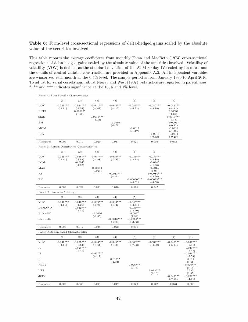
Table 6: Firm-level cross-sectional regressions of delta-hedged gains scaled by the absolutevalue of the securities involved

This table reports the average coefficients from monthly Fama and MacBeth (1973) cross-sectionalregressions of delta-hedged gains scaled by the absolute value of the securities involved. Volatility ofvolatility (VOV) is defined as the standard deviation of the ATM 30-day IV scaled by its mean andthe details of control variable construction are provided in Appendix A.2. All independent variablesare winsorized each month at the 0.5% level. The sample period is from January 1996 to April 2016.To adjust for serial correlation, robust Newey and West (1987) t-statistics are reported in parentheses.*, ** and *** indicates significance at the 10, 5 and 1% level.

Panel A: Firm-Specific Characteristics

(1) (2) (3) (4) (5) (6) (7)

VOV -0.041*** -0.044*** -0.041*** -0.043*** -0.043*** -0.040*** -0.044***(-4.11) (-4.58) (-4.08) (-4.12) (-4.32) (-3.89) (-4.41)

BETA 0.00082* 0.00052(1.67) (1.05)

SIZE 0.0015*** 0.0013***(4.02) (3.78)

BM -0.0016 -0.00057(-0.79) (-0.33)

MOM -0.0017 -0.0016(-1.47) (-1.50)

REV -0.0013 -0.0011(-0.32) (-0.29)

R-squared 0.009 0.019 0.020 0.017 0.021 0.019 0.053

Panel B: Return Distribution Characteristics

(1) (2) (3) (4) (5) (6)

VOV -0.041*** -0.036*** -0.047*** -0.039*** -0.034*** -0.035***(-4.11) (-3.83) (-4.98) (-3.83) (-3.13) (-3.85)

IVOL -0.094* -0.094*(-1.92) (-1.96)

MAX 0.00011 0.0044(0.025) (1.03)

RS -0.0013*** -0.00084***(-4.04) (-3.36)

RK -0.00030*** -0.00023***(-5.31) (-4.68)

R-squared 0.009 0.024 0.021 0.016 0.018 0.047

Panel C: Limits to Arbitrage

(1) (2) (3) (4) (5)

VOV -0.041*** -0.042*** -0.039*** -0.044*** -0.045***(-4.11) (-4.21) (-3.94) (-4.47) (-4.71)

DEMAND -0.042*** -0.036***(-4.47) (-3.20)

BID ASK -0.0096 0.0097(-1.35) (1.58)

LN ILLIQ -0.0016*** -0.0016***(-3.93) (-3.83)

R-squared 0.009 0.017 0.018 0.022 0.036

Panel D:Option-based Characteristics

(1) (2) (3) (4) (5) (6) (7) (8)

VOV -0.041*** -0.035*** -0.044*** -0.045*** -0.060*** -0.039*** -0.048*** -0.061***(-4.11) (-3.64) (-4.61) (-4.30) (-7.03) (-4.00) (-5.11) (-6.41)

IV -0.025*** -0.023***(-5.47) (-5.43)

IS -0.037*** -0.044***(-4.17) (-5.53)

IK 0.015** 0.011(2.02) (1.61)

RV IV 0.026*** 0.020***(7.74) (5.15)

VTS 0.073*** 0.020*(6.10) (1.85)

dCIV -0.042*** -0.026***(-7.58) (-4.11)

R-squared 0.009 0.039 0.021 0.017 0.022 0.027 0.023 0.088

42

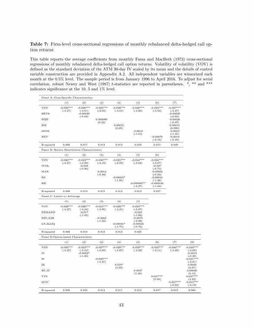
Table 7: Firm-level cross-sectional regressions of monthly rebalanced delta-hedged call op-tion returns

This table reports the average coefficients from monthly Fama and MacBeth (1973) cross-sectionalregressions of monthly rebalanced delta-hedged call option returns. Volatility of volatility (VOV) isdefined as the standard deviation of the ATM 30-day IV scaled by its mean and the details of controlvariable construction are provided in Appendix A.2. All independent variables are winsorized eachmonth at the 0.5% level. The sample period is from January 1996 to April 2016. To adjust for serialcorrelation, robust Newey and West (1987) t-statistics are reported in parentheses. *, ** and ***indicates significance at the 10, 5 and 1% level.

Panel A: Firm-Specific Characteristics

(1) (2) (3) (4) (5) (6) (7)

VOV -0.026*** -0.026*** -0.025*** -0.028*** -0.026*** -0.025*** -0.027***(-4.27) (-4.41) (-3.93) (-4.51) (-4.06) (-3.92) (-4.27)

BETA -0.00020 -0.00029(-0.62) (-0.90)

SIZE 0.000080 -0.00026(0.32) (-0.97)

BM 0.00041 0.00014(0.29) (0.098)

MOM -0.0016 -0.0013(-1.53) (-1.35)

REV -0.00070 -0.0019(-0.18) (-0.49)

R-squared 0.006 0.017 0.013 0.013 0.018 0.015 0.049

Panel B: Return Distribution Characteristics

(1) (2) (3) (4) (5) (6)

VOV -0.026*** -0.023*** -0.026*** -0.025*** -0.024*** -0.024***(-4.27) (-3.30) (-4.19) (-3.93) (-3.64) (-3.67)

IVOL -0.038 -0.027(-0.96) (-0.74)

MAX -0.0014 -0.00092(-0.34) (-0.22)

RS -0.00065* -0.00044(-1.85) (-1.36)

RK -0.000085** -0.000046(-2.27) (-1.24)

R-squared 0.006 0.019 0.015 0.012 0.013 0.037

Panel C: Limits to Arbitrage

(1) (2) (3) (4) (5)

VOV -0.026*** -0.026*** -0.024*** -0.026*** -0.024***(-4.27) (-4.24) (-3.95) (-4.21) (-3.97)

DEMAND -0.017 -0.023(-1.45) (-1.06)

BID ASK -0.0084 -0.0075(-1.50) (-0.98)

LN ILLIQ -0.00041* -0.00023(-1.75) (-0.76)

R-squared 0.006 0.010 0.013 0.013 0.025

Panel D:Option-based Characteristics

(1) (2) (3) (4) (5) (6) (7) (8)

VOV -0.026*** -0.023*** -0.027*** -0.029*** -0.029*** -0.022*** -0.026*** -0.024***(-4.27) (-3.44) (-4.60) (-4.87) (-4.92) (-3.11) (-4.38) (-3.63)

IV -0.0062* -0.0015(-1.90) (-0.39)

IS -0.020*** -0.021***(-3.27) (-3.91)

IK 0.010* 0.0049(1.90) (0.87)

RV IV 0.0037 0.00030(1.56) (0.12)

VTS 0.047*** 0.037***(5.39) (4.35)

dCIV -0.027*** -0.015***(-6.02) (-3.19)

R-squared 0.006 0.025 0.014 0.011 0.013 0.017 0.015 0.060

43

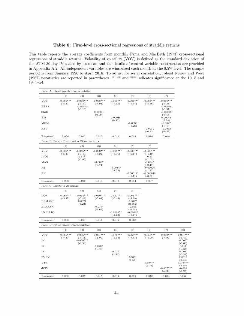
Table 8: Firm-level cross-sectional regressions of straddle returns

This table reports the average coefficients from monthly Fama and MacBeth (1973) cross-sectionalregressions of straddle returns. Volatility of volatility (VOV) is defined as the standard deviation ofthe ATM 30-day IV scaled by its mean and the details of control variable construction are providedin Appendix A.2. All independent variables are winsorized each month at the 0.5% level. The sampleperiod is from January 1996 to April 2016. To adjust for serial correlation, robust Newey and West(1987) t-statistics are reported in parentheses. *, ** and *** indicates significance at the 10, 5 and1% level.

Panel A: Firm-Specific Characteristics

(1) (2) (3) (4) (5) (6) (7)

VOV -0.065*** -0.063*** -0.063*** -0.069*** -0.065*** -0.063*** -0.066***(-5.47) (-5.30) (-4.94) (-5.95) (-5.34) (-5.16) (-5.31)

BETA -0.00073 -0.00078(-1.10) (-1.31)

SIZE 0.00061 -0.00036(0.99) (-0.58)

BM 0.00088 0.00043(0.30) (0.14)

MOM -0.0030 -0.0027(-1.28) (-1.18)

REV -0.0011 -0.0032(-0.13) (-0.37)

R-squared 0.006 0.017 0.015 0.014 0.018 0.016 0.050

Panel B: Return Distribution Characteristics

(1) (2) (3) (4) (5) (6)

VOV -0.065*** -0.055*** -0.063*** -0.065*** -0.063*** -0.060***(-5.47) (-3.49) (-5.22) (-5.36) (-5.17) (-4.49)

IVOL -0.17** -0.11(-2.00) (-1.62)

MAX -0.0067 -0.0042(-0.74) (-0.47)

RS -0.0014* -0.00095(-1.72) (-1.27)

RK -0.00014* -0.000048(-1.71) (-0.61)

R-squared 0.006 0.020 0.015 0.013 0.014 0.037

Panel C: Limits to Arbitrage

(1) (2) (3) (4) (5)

VOV -0.065*** -0.064*** -0.060*** -0.067*** -0.061***(-5.47) (-5.42) (-5.04) (-5.44) (-5.29)

DEMAND 0.0071 0.0027(0.22) (0.055)

BID ASK -0.019* -0.015(-1.65) (-0.94)

LN ILLIQ -0.0013** -0.00087(-2.23) (-1.21)

R-squared 0.006 0.011 0.014 0.017 0.028

Panel D:Option-based Characteristics

(1) (2) (3) (4) (5) (6) (7) (8)

VOV -0.065*** -0.056*** -0.061*** -0.071*** -0.068*** -0.058*** -0.060*** -0.051***(-5.47) (-4.11) (-5.00) (-6.08) (-5.43) (-4.00) (-4.97) (-3.49)

IV -0.020*** -0.0057(-2.98) (-0.68)

IS 0.020* 0.017(1.73) (1.52)

IK 0.015 -0.0041(1.33) (-0.31)

RV IV 0.0081 0.0018(1.57) (0.34)

VTS 0.10*** 0.078***(5.72) (3.45)

dCIV -0.037*** -0.014(-4.33) (-1.25)

R-squared 0.006 0.027 0.015 0.012 0.016 0.018 0.014 0.062

44

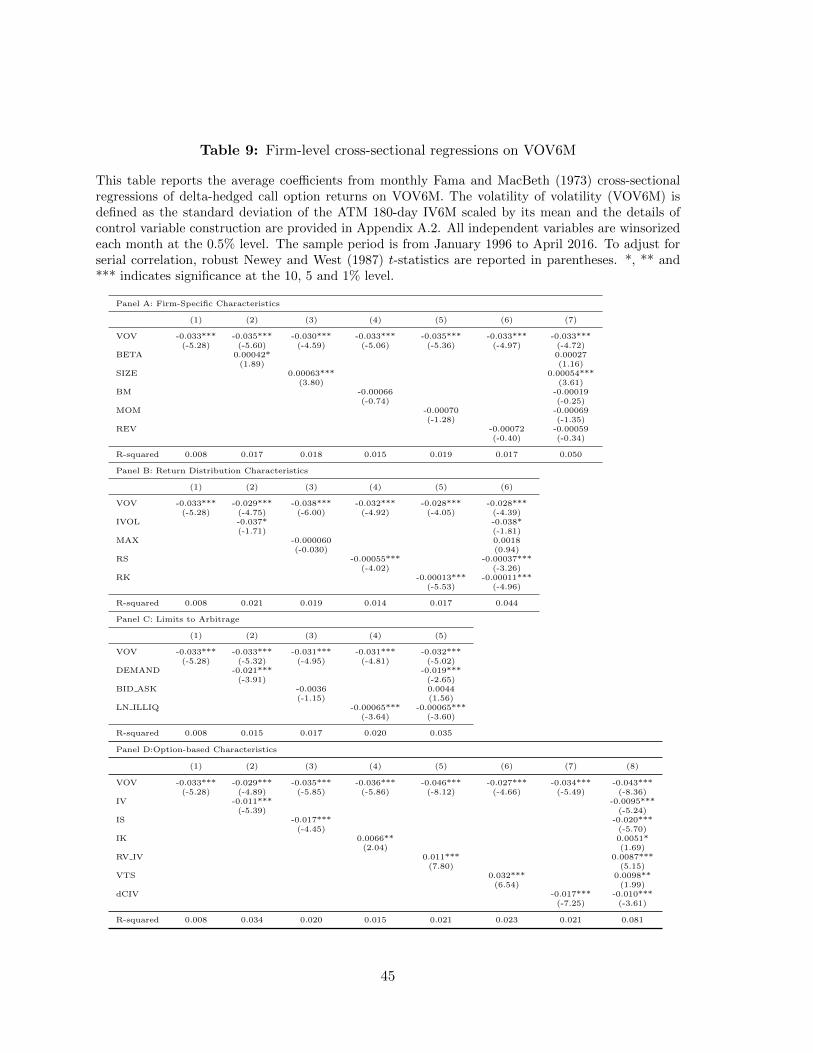
Table 9: Firm-level cross-sectional regressions on VOV6M

This table reports the average coefficients from monthly Fama and MacBeth (1973) cross-sectionalregressions of delta-hedged call option returns on VOV6M. The volatility of volatility (VOV6M) isdefined as the standard deviation of the ATM 180-day IV6M scaled by its mean and the details ofcontrol variable construction are provided in Appendix A.2. All independent variables are winsorizedeach month at the 0.5% level. The sample period is from January 1996 to April 2016. To adjust forserial correlation, robust Newey and West (1987) t-statistics are reported in parentheses. *, ** and*** indicates significance at the 10, 5 and 1% level.

Panel A: Firm-Specific Characteristics

(1) (2) (3) (4) (5) (6) (7)

VOV -0.033*** -0.035*** -0.030*** -0.033*** -0.035*** -0.033*** -0.033***(-5.28) (-5.60) (-4.59) (-5.06) (-5.36) (-4.97) (-4.72)

BETA 0.00042* 0.00027(1.89) (1.16)

SIZE 0.00063*** 0.00054***(3.80) (3.61)

BM -0.00066 -0.00019(-0.74) (-0.25)

MOM -0.00070 -0.00069(-1.28) (-1.35)

REV -0.00072 -0.00059(-0.40) (-0.34)

R-squared 0.008 0.017 0.018 0.015 0.019 0.017 0.050

Panel B: Return Distribution Characteristics

(1) (2) (3) (4) (5) (6)

VOV -0.033*** -0.029*** -0.038*** -0.032*** -0.028*** -0.028***(-5.28) (-4.75) (-6.00) (-4.92) (-4.05) (-4.39)

IVOL -0.037* -0.038*(-1.71) (-1.81)

MAX -0.000060 0.0018(-0.030) (0.94)

RS -0.00055*** -0.00037***(-4.02) (-3.26)

RK -0.00013*** -0.00011***(-5.53) (-4.96)

R-squared 0.008 0.021 0.019 0.014 0.017 0.044

Panel C: Limits to Arbitrage

(1) (2) (3) (4) (5)

VOV -0.033*** -0.033*** -0.031*** -0.031*** -0.032***(-5.28) (-5.32) (-4.95) (-4.81) (-5.02)

DEMAND -0.021*** -0.019***(-3.91) (-2.65)

BID ASK -0.0036 0.0044(-1.15) (1.56)

LN ILLIQ -0.00065*** -0.00065***(-3.64) (-3.60)

R-squared 0.008 0.015 0.017 0.020 0.035

Panel D:Option-based Characteristics

(1) (2) (3) (4) (5) (6) (7) (8)

VOV -0.033*** -0.029*** -0.035*** -0.036*** -0.046*** -0.027*** -0.034*** -0.043***(-5.28) (-4.89) (-5.85) (-5.86) (-8.12) (-4.66) (-5.49) (-8.36)

IV -0.011*** -0.0095***(-5.39) (-5.24)

IS -0.017*** -0.020***(-4.45) (-5.70)

IK 0.0066** 0.0051*(2.04) (1.69)

RV IV 0.011*** 0.0087***(7.80) (5.15)

VTS 0.032*** 0.0098**(6.54) (1.99)

dCIV -0.017*** -0.010***(-7.25) (-3.61)

R-squared 0.008 0.034 0.020 0.015 0.021 0.023 0.021 0.081

45

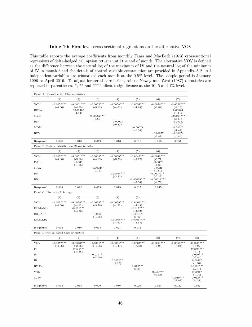
Table 10: Firm-level cross-sectional regressions on the alternative VOV

This table reports the average coefficients from monthly Fama and MacBeth (1973) cross-sectionalregressions of delta-hedged call option returns until the end of month. The alternative VOV is definedas the difference between the natural log of the maximum of IV and the natural log of the minimumof IV in month t and the details of control variable construction are provided in Appendix A.2. Allindependent variables are winsorized each month at the 0.5% level. The sample period is January1996 to April 2016. To adjust for serial correlation, robust Newey and West (1987) t-statistics arereported in parentheses. *, ** and *** indicates significance at the 10, 5 and 1% level.

Panel A: Firm-Specific Characteristics

(1) (2) (3) (4) (5) (6) (7)

VOV -0.0057*** -0.0061*** -0.0055*** -0.0058*** -0.0058*** -0.0056*** -0.0059***(-4.06) (-4.59) (-3.92) (-4.01) (-4.14) (-3.84) (-4.13)

BETA 0.00040* 0.00024(1.84) (1.11)

SIZE 0.00062*** 0.00051***(3.69) (3.47)

BM -0.00073 -0.00030(-0.82) (-0.40)

MOM -0.00071 -0.00070(-1.34) (-1.41)

REV -0.00077 -0.00074(-0.44) (-0.42)

R-squared 0.008 0.018 0.019 0.016 0.019 0.018 0.051

Panel B: Return Distribution Characteristics

(1) (2) (3) (4) (5) (6)

VOV -0.0057*** -0.0051*** -0.0064*** -0.0055*** -0.0047*** -0.0048***(-4.06) (-3.88) (-4.89) (-3.78) (-3.12) (-3.77)

IVOL -0.035 -0.035*(-1.63) (-1.66)

MAX 0.00024 0.0021(0.12) (1.11)

RS -0.00054*** -0.00037***(-3.91) (-3.29)

RK -0.00013*** -0.00011***(-5.38) (-4.79)

R-squared 0.008 0.022 0.019 0.015 0.017 0.045

Panel C: Limits to Arbitrage

(1) (2) (3) (4) (5)

VOV -0.0057*** -0.0058*** -0.0054*** -0.0059*** -0.0062***(-4.06) (-4.12) (-3.78) (-4.22) (-4.49)

DEMAND -0.018*** -0.017***(-4.53) (-3.02)

BID ASK -0.0035 0.0048*(-1.08) (1.69)

LN ILLIQ -0.00065*** -0.00067***(-3.63) (-3.68)

R-squared 0.008 0.016 0.018 0.021 0.035

Panel D:Option-based Characteristics

(1) (2) (3) (4) (5) (6) (7) (8)

VOV -0.0057*** -0.0048*** -0.0061*** -0.0064*** -0.0087*** -0.0054*** -0.0066*** -0.0088***(-4.06) (-3.66) (-4.56) (-4.47) (-7.38) (-3.93) (-5.01) (-6.92)

IV -0.011*** -0.0094***(-5.38) (-5.11)

IS -0.017*** -0.020***(-4.49) (-5.84)

IK 0.0071** 0.0058*(2.22) (1.90)

RV IV 0.012*** 0.0091***(8.09) (5.31)

VTS 0.033*** 0.0095*(6.43) (1.94)

dCIV -0.019*** -0.012***(-7.92) (-4.21)

R-squared 0.008 0.035 0.020 0.016 0.021 0.024 0.022 0.082

46

Table 11: Univariate portfolios sorted on VOV

This table reports the average return of holding delta-hedged call option portfolios on volatility ofvolatility (VOV). At the end of each month, we rank the delta-hedged option portfolios into 5 decilesbased on VOV and then calculate the equal-weighted monthly returns of those 5 portfolios. Thistable also reports the difference in the average returns of the low and the high VOV decile portfoliosin the “High-Low ” row. VOV is defined as the standard deviation of the ATM 30-day IV scaledby its mean. The risk-adjusted average returns are also reported in the column 3 to column 6. Therisk factors including Fama and French (1993) three factors (MKT, SMB, HML), Carhart (1997)momentum factor (UMD) and Fama and French (2015) five factors (RMW, CMA) are obtained fromthe Kenneth R. French Data Library. The sample period is from January 1996 to April 2016. Therobust Newey and West (1987) t-statistics of the high-row portfolios are reported in parentheses. *,** and *** indicates significance at the 10, 5 and 1% level.

Raw return CAPM alpha Three-Factor alpha Four-Factor alpha Five-Factor alpha

Low -0.24 -0.22 -0.23 -0.26 -0.212 -0.24 -0.22 -0.22 -0.26 -0.213 -0.24 -0.22 -0.23 -0.25 -0.224 -0.32 -0.30 -0.31 -0.33 -0.31High -0.40 -0.38 -0.39 -0.41 -0.39High-Low -0.16*** -0.16*** -0.17*** -0.15** -0.18***

(-2.90) (-2.83) (-3.06) (-2.60) (-3.23)

Table 12: Firm-level cross-sectional regressions of VOV

This table reports the average coefficients from monthly Fama and MacBeth (1973) cross-sectionalregressions of VOV. All independent variables are winsorized each month at the 0.5% level. Thesample period is January 1996 to April 2016. To adjust for serial correlation, robust Newey and West(1987) t-statistics are reported in parentheses. *, ** and *** indicates significance at the 10, 5 and1% level.

(1) (2) (3) (4) (5) (6) (7) (8) (9) (10) (11) (12) (13) (14) (15) (16) (17) (18)

VOV 0.44*** 0.40***(19.9) (21.9)

BETA -0.0025*** -0.00068***(-5.10) (-4.79)

SIZE -0.0047*** -0.0012*(-6.04) (-1.95)

BM 0.0073*** 0.0016***(5.70) (5.24)

MOM -0.0057*** -0.0029***(-4.39) (-6.48)

REV 0.0055** 0.0016(2.55) (1.19)

IVOL -0.091* -0.12**(-1.69) (-2.02)

MAX 0.0017 0.0034***(0.84) (2.67)

RS 0.0034*** 0.0017***(10.4) (12.9)

RK 0.00049*** 0.00026***(14.4) (14.1)

LN ILLIQ 0.0036*** 0.00036(5.61) (0.68)

IV 0.032*** -0.014**(6.68) (-2.59)

IS -0.00068 -0.0038(-0.13) (-1.42)

IK 0.070*** 0.051***(15.4) (15.3)

RV IV -0.044*** -0.028***(-5.49) (-5.24)

VTS -0.20*** -0.100***(-10.8) (-14.2)

dCIV 0.022*** 0.0014(9.27) (0.63)

R-squared 0.196 0.003 0.015 0.004 0.003 0.002 0.005 0.002 0.005 0.009 0.015 0.015 0.005 0.018 0.021 0.051 0.008 0.253

47

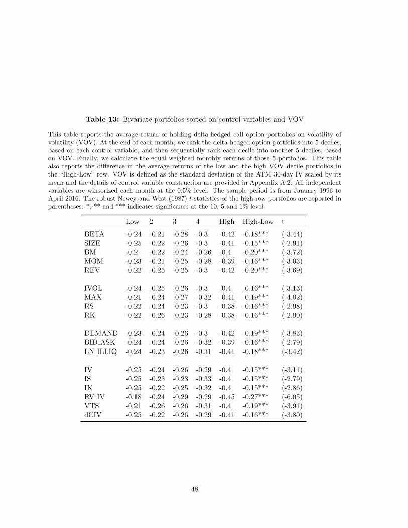
Table 13: Bivariate portfolios sorted on control variables and VOV

This table reports the average return of holding delta-hedged call option portfolios on volatility ofvolatility (VOV). At the end of each month, we rank the delta-hedged option portfolios into 5 deciles,based on each control variable, and then sequentially rank each decile into another 5 deciles, basedon VOV. Finally, we calculate the equal-weighted monthly returns of those 5 portfolios. This tablealso reports the difference in the average returns of the low and the high VOV decile portfolios inthe “High-Low” row. VOV is defined as the standard deviation of the ATM 30-day IV scaled by itsmean and the details of control variable construction are provided in Appendix A.2. All independentvariables are winsorized each month at the 0.5% level. The sample period is from January 1996 toApril 2016. The robust Newey and West (1987) t-statistics of the high-row portfolios are reported inparentheses. *, ** and *** indicates significance at the 10, 5 and 1% level.

Low 2 3 4 High High-Low t

BETA -0.24 -0.21 -0.28 -0.3 -0.42 -0.18*** (-3.44)SIZE -0.25 -0.22 -0.26 -0.3 -0.41 -0.15*** (-2.91)BM -0.2 -0.22 -0.24 -0.26 -0.4 -0.20*** (-3.72)MOM -0.23 -0.21 -0.25 -0.28 -0.39 -0.16*** (-3.03)REV -0.22 -0.25 -0.25 -0.3 -0.42 -0.20*** (-3.69)

IVOL -0.24 -0.25 -0.26 -0.3 -0.4 -0.16*** (-3.13)MAX -0.21 -0.24 -0.27 -0.32 -0.41 -0.19*** (-4.02)RS -0.22 -0.24 -0.23 -0.3 -0.38 -0.16*** (-2.98)RK -0.22 -0.26 -0.23 -0.28 -0.38 -0.16*** (-2.90)

DEMAND -0.23 -0.24 -0.26 -0.3 -0.42 -0.19*** (-3.83)BID ASK -0.24 -0.24 -0.26 -0.32 -0.39 -0.16*** (-2.79)LN ILLIQ -0.24 -0.23 -0.26 -0.31 -0.41 -0.18*** (-3.42)

IV -0.25 -0.24 -0.26 -0.29 -0.4 -0.15*** (-3.11)IS -0.25 -0.23 -0.23 -0.33 -0.4 -0.15*** (-2.79)IK -0.25 -0.22 -0.25 -0.32 -0.4 -0.15*** (-2.86)RV IV -0.18 -0.24 -0.29 -0.29 -0.45 -0.27*** (-6.05)VTS -0.21 -0.26 -0.26 -0.31 -0.4 -0.19*** (-3.91)dCIV -0.25 -0.22 -0.26 -0.29 -0.41 -0.16*** (-3.80)

48

Cross Section of Option Returns and Volatility-of-Volatility

Internet Appendix

1

Table IA.1: Firm-level cross-sectional regressions after controlling for VOL-of-VOL in Caoet al. (2017)

This table reports the average coefficients from monthly Fama and MacBeth (1973) cross-sectionalregressions of delta-hedged call option returns. Volatility of volatility (VOV) is defined as the standarddeviation of the ATM 30-day IV scaled its mean and the details of control variable construction areprovided in Appendix A.2. In line with Cao et al. (2017), we obtain estimates of daily volatility foreach stock in each month by applying from the EGARCH (1,1) model to a rolling window of past12-month daily stock returns and VOL-of-VOL is measured as the standard deviation of percentagechange in the daily realized volatility over one month. All independent variables are winsorized eachmonth at the 0.5% level. The sample period is from January 1996 to April 2016. To adjust for serialcorrelation, robust Newey and West (1987) t-statistics are reported in parentheses. *, ** and ***indicates significance at the 10, 5 and 1% level.

(1) (2) (3)

VOV -0.018*** -0.017***(-4.20) (-3.57)

VOL-of-VOL -4.2e-06*** -3.7e-06**(-2.83) (-2.49)

2

Table IA.2: Firm-level cross-sectional regressions on the unscaled VOV

This table reports the average coefficients from monthly Fama and MacBeth (1973) cross-sectionalregressions of delta-hedged call option returns. The unscaled volatility of volatility (unscaled VOV) isdefined as the standard deviation of the ATM 30-day IV and the details of control variable constructionare provided in Appendix A.2. All independent variables are winsorized each month at the 0.5% level.The sample period is from January 1996 to April 2016. To adjust for serial correlation, robust Neweyand West (1987) t-statistics are reported in parentheses. *, ** and *** indicates significance at the10, 5 and 1% level.

Panel A: Firm-Specific Characteristics

(1) (2) (3) (4) (5) (6) (7)

VOV -0.055*** -0.061*** -0.053*** -0.055*** -0.057*** -0.056*** -0.063***(-5.49) (-6.55) (-5.03) (-5.46) (-5.54) (-5.87) (-6.31)

BETA 0.00059** 0.00041*(2.50) (1.67)

SIZE 0.00033* 0.00023(1.84) (1.45)

BM -0.00098 -0.00052(-1.12) (-0.68)

MOM -0.00040 -0.00037(-0.73) (-0.75)

REV -0.00083 -0.00080(-0.47) (-0.46)

R-squared 0.018 0.027 0.027 0.025 0.030 0.027 0.059

Panel B: Return Distribution Characteristics

(1) (2) (3) (4) (5) (6)

VOV -0.055*** -0.058*** -0.063*** -0.051*** -0.048*** -0.058***(-5.49) (-6.63) (-6.62) (-4.80) (-4.37) (-6.42)

IVOL 0.016 0.013(0.79) (0.67)

MAX 0.00031 0.0014(0.16) (0.74)

RS -0.00051*** -0.00034***(-3.69) (-3.09)

RK -0.00012*** -0.000098***(-4.64) (-4.36)

R-squared 0.018 0.029 0.030 0.025 0.026 0.052

Panel C: Limits to Arbitrage

(1) (2) (3) (4) (5)

VOV -0.055*** -0.055*** -0.055*** -0.053*** -0.053***(-5.49) (-5.60) (-5.49) (-5.29) (-5.31)

DEMAND -0.021*** -0.018***(-3.75) (-2.89)

BID ASK -0.0030 0.0034(-0.97) (1.28)

LN ILLIQ -0.00042** -0.00038**(-2.22) (-1.98)

R-squared 0.018 0.025 0.027 0.030 0.044

Panel D:Option-based Characteristics

(1) (2) (3) (4) (5) (6) (7) (8)

VOV -0.055*** -0.031*** -0.059*** -0.057*** -0.067*** -0.048*** -0.059*** -0.056***(-5.49) (-3.22) (-6.26) (-5.57) (-7.58) (-4.91) (-5.77) (-6.34)

IV -0.0081*** -0.0049**(-3.96) (-2.49)

IS -0.019*** -0.020***(-5.32) (-6.07)

IK 0.0081** 0.0047(2.57) (1.56)

RV IV 0.012*** 0.0091***(7.96) (5.37)

VTS 0.030*** 0.0099**(6.42) (2.03)

dCIV -0.021*** -0.013***(-8.22) (-4.70)

R-squared 0.018 0.039 0.030 0.026 0.031 0.031 0.032 0.085

3

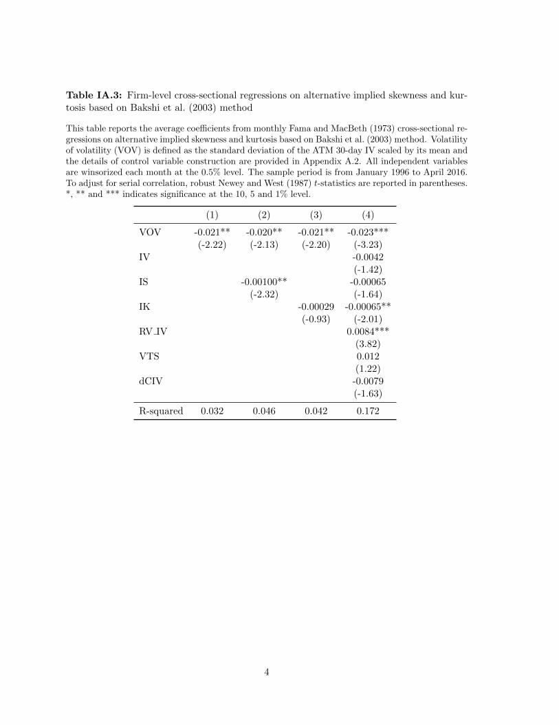
Table IA.3: Firm-level cross-sectional regressions on alternative implied skewness and kur-tosis based on Bakshi et al. (2003) method

This table reports the average coefficients from monthly Fama and MacBeth (1973) cross-sectional re-gressions on alternative implied skewness and kurtosis based on Bakshi et al. (2003) method. Volatilityof volatility (VOV) is defined as the standard deviation of the ATM 30-day IV scaled by its mean andthe details of control variable construction are provided in Appendix A.2. All independent variablesare winsorized each month at the 0.5% level. The sample period is from January 1996 to April 2016.To adjust for serial correlation, robust Newey and West (1987) t-statistics are reported in parentheses.*, ** and *** indicates significance at the 10, 5 and 1% level.

(1) (2) (3) (4)

VOV -0.021** -0.020** -0.021** -0.023***(-2.22) (-2.13) (-2.20) (-3.23)

IV -0.0042(-1.42)

IS -0.00100** -0.00065(-2.32) (-1.64)

IK -0.00029 -0.00065**(-0.93) (-2.01)

RV IV 0.0084***(3.82)

VTS 0.012(1.22)

dCIV -0.0079(-1.63)

R-squared 0.032 0.046 0.042 0.172

4

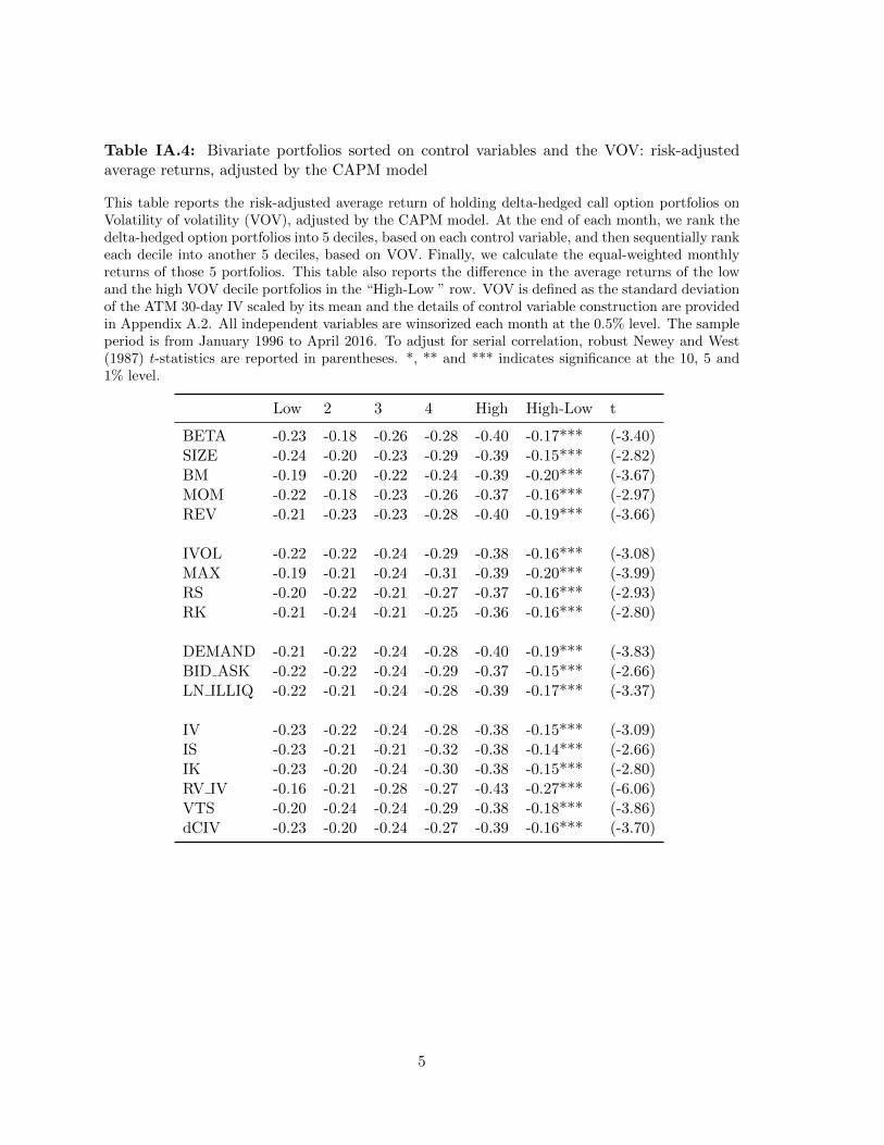
Table IA.4: Bivariate portfolios sorted on control variables and the VOV: risk-adjustedaverage returns, adjusted by the CAPM model

This table reports the risk-adjusted average return of holding delta-hedged call option portfolios onVolatility of volatility (VOV), adjusted by the CAPM model. At the end of each month, we rank thedelta-hedged option portfolios into 5 deciles, based on each control variable, and then sequentially rankeach decile into another 5 deciles, based on VOV. Finally, we calculate the equal-weighted monthlyreturns of those 5 portfolios. This table also reports the difference in the average returns of the lowand the high VOV decile portfolios in the “High-Low ” row. VOV is defined as the standard deviationof the ATM 30-day IV scaled by its mean and the details of control variable construction are providedin Appendix A.2. All independent variables are winsorized each month at the 0.5% level. The sampleperiod is from January 1996 to April 2016. To adjust for serial correlation, robust Newey and West(1987) t-statistics are reported in parentheses. *, ** and *** indicates significance at the 10, 5 and1% level.

Low 2 3 4 High High-Low t

BETA -0.23 -0.18 -0.26 -0.28 -0.40 -0.17*** (-3.40)SIZE -0.24 -0.20 -0.23 -0.29 -0.39 -0.15*** (-2.82)BM -0.19 -0.20 -0.22 -0.24 -0.39 -0.20*** (-3.67)MOM -0.22 -0.18 -0.23 -0.26 -0.37 -0.16*** (-2.97)REV -0.21 -0.23 -0.23 -0.28 -0.40 -0.19*** (-3.66)

IVOL -0.22 -0.22 -0.24 -0.29 -0.38 -0.16*** (-3.08)MAX -0.19 -0.21 -0.24 -0.31 -0.39 -0.20*** (-3.99)RS -0.20 -0.22 -0.21 -0.27 -0.37 -0.16*** (-2.93)RK -0.21 -0.24 -0.21 -0.25 -0.36 -0.16*** (-2.80)

DEMAND -0.21 -0.22 -0.24 -0.28 -0.40 -0.19*** (-3.83)BID ASK -0.22 -0.22 -0.24 -0.29 -0.37 -0.15*** (-2.66)LN ILLIQ -0.22 -0.21 -0.24 -0.28 -0.39 -0.17*** (-3.37)

IV -0.23 -0.22 -0.24 -0.28 -0.38 -0.15*** (-3.09)IS -0.23 -0.21 -0.21 -0.32 -0.38 -0.14*** (-2.66)IK -0.23 -0.20 -0.24 -0.30 -0.38 -0.15*** (-2.80)RV IV -0.16 -0.21 -0.28 -0.27 -0.43 -0.27*** (-6.06)VTS -0.20 -0.24 -0.24 -0.29 -0.38 -0.18*** (-3.86)dCIV -0.23 -0.20 -0.24 -0.27 -0.39 -0.16*** (-3.70)

5

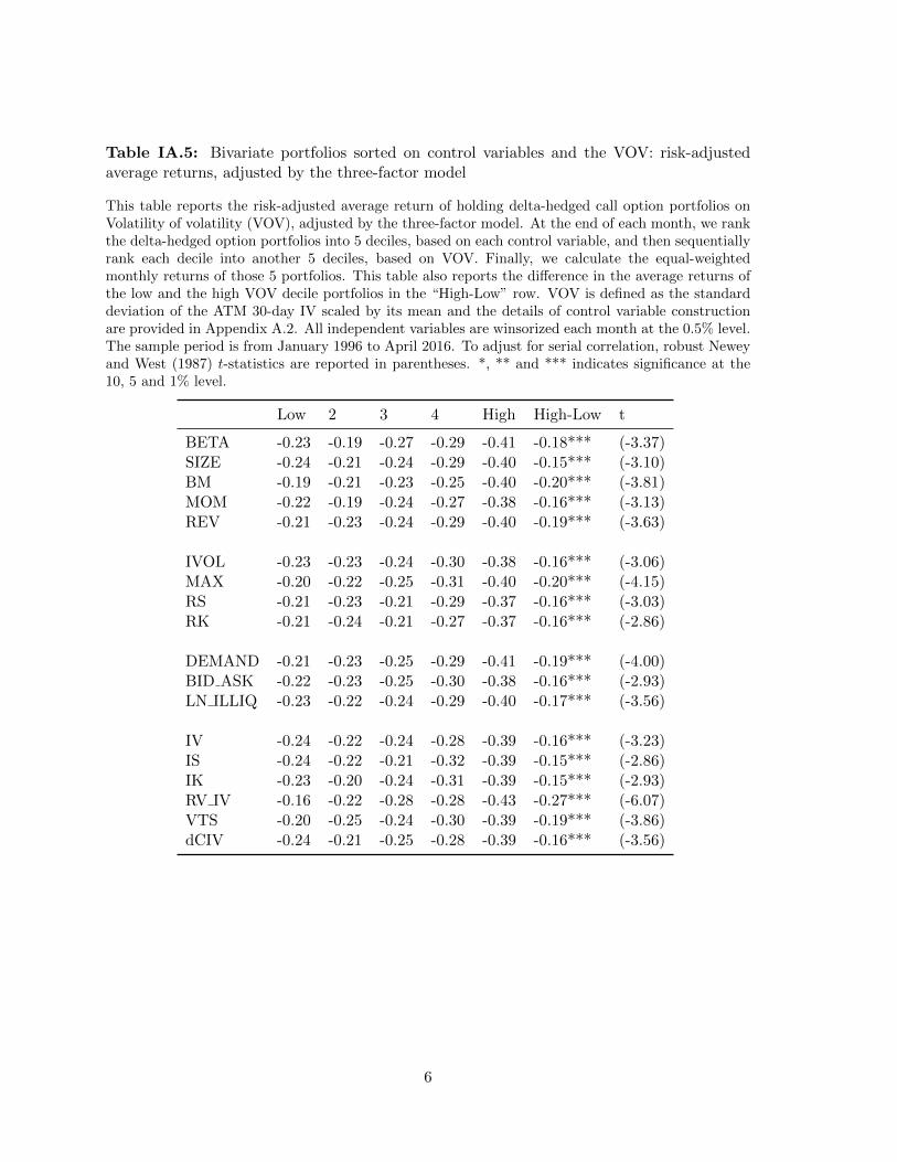
Table IA.5: Bivariate portfolios sorted on control variables and the VOV: risk-adjustedaverage returns, adjusted by the three-factor model

This table reports the risk-adjusted average return of holding delta-hedged call option portfolios onVolatility of volatility (VOV), adjusted by the three-factor model. At the end of each month, we rankthe delta-hedged option portfolios into 5 deciles, based on each control variable, and then sequentiallyrank each decile into another 5 deciles, based on VOV. Finally, we calculate the equal-weightedmonthly returns of those 5 portfolios. This table also reports the difference in the average returns ofthe low and the high VOV decile portfolios in the “High-Low” row. VOV is defined as the standarddeviation of the ATM 30-day IV scaled by its mean and the details of control variable constructionare provided in Appendix A.2. All independent variables are winsorized each month at the 0.5% level.The sample period is from January 1996 to April 2016. To adjust for serial correlation, robust Neweyand West (1987) t-statistics are reported in parentheses. *, ** and *** indicates significance at the10, 5 and 1% level.

Low 2 3 4 High High-Low t

BETA -0.23 -0.19 -0.27 -0.29 -0.41 -0.18*** (-3.37)SIZE -0.24 -0.21 -0.24 -0.29 -0.40 -0.15*** (-3.10)BM -0.19 -0.21 -0.23 -0.25 -0.40 -0.20*** (-3.81)MOM -0.22 -0.19 -0.24 -0.27 -0.38 -0.16*** (-3.13)REV -0.21 -0.23 -0.24 -0.29 -0.40 -0.19*** (-3.63)

IVOL -0.23 -0.23 -0.24 -0.30 -0.38 -0.16*** (-3.06)MAX -0.20 -0.22 -0.25 -0.31 -0.40 -0.20*** (-4.15)RS -0.21 -0.23 -0.21 -0.29 -0.37 -0.16*** (-3.03)RK -0.21 -0.24 -0.21 -0.27 -0.37 -0.16*** (-2.86)

DEMAND -0.21 -0.23 -0.25 -0.29 -0.41 -0.19*** (-4.00)BID ASK -0.22 -0.23 -0.25 -0.30 -0.38 -0.16*** (-2.93)LN ILLIQ -0.23 -0.22 -0.24 -0.29 -0.40 -0.17*** (-3.56)

IV -0.24 -0.22 -0.24 -0.28 -0.39 -0.16*** (-3.23)IS -0.24 -0.22 -0.21 -0.32 -0.39 -0.15*** (-2.86)IK -0.23 -0.20 -0.24 -0.31 -0.39 -0.15*** (-2.93)RV IV -0.16 -0.22 -0.28 -0.28 -0.43 -0.27*** (-6.07)VTS -0.20 -0.25 -0.24 -0.30 -0.39 -0.19*** (-3.86)dCIV -0.24 -0.21 -0.25 -0.28 -0.39 -0.16*** (-3.56)

6

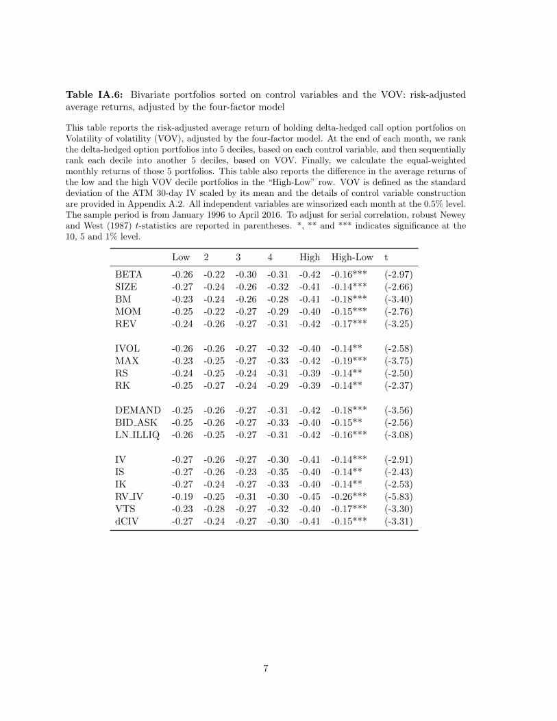
Table IA.6: Bivariate portfolios sorted on control variables and the VOV: risk-adjustedaverage returns, adjusted by the four-factor model

This table reports the risk-adjusted average return of holding delta-hedged call option portfolios onVolatility of volatility (VOV), adjusted by the four-factor model. At the end of each month, we rankthe delta-hedged option portfolios into 5 deciles, based on each control variable, and then sequentiallyrank each decile into another 5 deciles, based on VOV. Finally, we calculate the equal-weightedmonthly returns of those 5 portfolios. This table also reports the difference in the average returns ofthe low and the high VOV decile portfolios in the “High-Low” row. VOV is defined as the standarddeviation of the ATM 30-day IV scaled by its mean and the details of control variable constructionare provided in Appendix A.2. All independent variables are winsorized each month at the 0.5% level.The sample period is from January 1996 to April 2016. To adjust for serial correlation, robust Neweyand West (1987) t-statistics are reported in parentheses. *, ** and *** indicates significance at the10, 5 and 1% level.

Low 2 3 4 High High-Low t

BETA -0.26 -0.22 -0.30 -0.31 -0.42 -0.16*** (-2.97)SIZE -0.27 -0.24 -0.26 -0.32 -0.41 -0.14*** (-2.66)BM -0.23 -0.24 -0.26 -0.28 -0.41 -0.18*** (-3.40)MOM -0.25 -0.22 -0.27 -0.29 -0.40 -0.15*** (-2.76)REV -0.24 -0.26 -0.27 -0.31 -0.42 -0.17*** (-3.25)

IVOL -0.26 -0.26 -0.27 -0.32 -0.40 -0.14** (-2.58)MAX -0.23 -0.25 -0.27 -0.33 -0.42 -0.19*** (-3.75)RS -0.24 -0.25 -0.24 -0.31 -0.39 -0.14** (-2.50)RK -0.25 -0.27 -0.24 -0.29 -0.39 -0.14** (-2.37)

DEMAND -0.25 -0.26 -0.27 -0.31 -0.42 -0.18*** (-3.56)BID ASK -0.25 -0.26 -0.27 -0.33 -0.40 -0.15** (-2.56)LN ILLIQ -0.26 -0.25 -0.27 -0.31 -0.42 -0.16*** (-3.08)

IV -0.27 -0.26 -0.27 -0.30 -0.41 -0.14*** (-2.91)IS -0.27 -0.26 -0.23 -0.35 -0.40 -0.14** (-2.43)IK -0.27 -0.24 -0.27 -0.33 -0.40 -0.14** (-2.53)RV IV -0.19 -0.25 -0.31 -0.30 -0.45 -0.26*** (-5.83)VTS -0.23 -0.28 -0.27 -0.32 -0.40 -0.17*** (-3.30)dCIV -0.27 -0.24 -0.27 -0.30 -0.41 -0.15*** (-3.31)

7

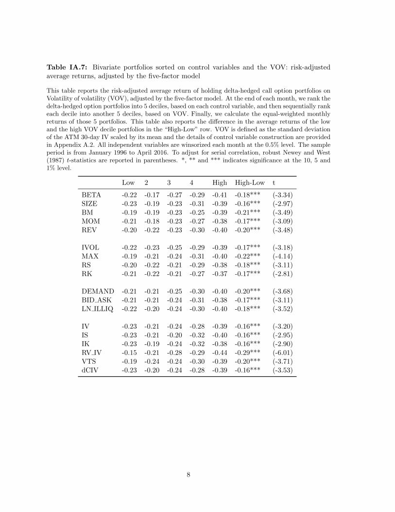
Table IA.7: Bivariate portfolios sorted on control variables and the VOV: risk-adjustedaverage returns, adjusted by the five-factor model

This table reports the risk-adjusted average return of holding delta-hedged call option portfolios onVolatility of volatility (VOV), adjusted by the five-factor model. At the end of each month, we rank thedelta-hedged option portfolios into 5 deciles, based on each control variable, and then sequentially rankeach decile into another 5 deciles, based on VOV. Finally, we calculate the equal-weighted monthlyreturns of those 5 portfolios. This table also reports the difference in the average returns of the lowand the high VOV decile portfolios in the “High-Low” row. VOV is defined as the standard deviationof the ATM 30-day IV scaled by its mean and the details of control variable construction are providedin Appendix A.2. All independent variables are winsorized each month at the 0.5% level. The sampleperiod is from January 1996 to April 2016. To adjust for serial correlation, robust Newey and West(1987) t-statistics are reported in parentheses. *, ** and *** indicates significance at the 10, 5 and1% level.

Low 2 3 4 High High-Low t

BETA -0.22 -0.17 -0.27 -0.29 -0.41 -0.18*** (-3.34)SIZE -0.23 -0.19 -0.23 -0.31 -0.39 -0.16*** (-2.97)BM -0.19 -0.19 -0.23 -0.25 -0.39 -0.21*** (-3.49)MOM -0.21 -0.18 -0.23 -0.27 -0.38 -0.17*** (-3.09)REV -0.20 -0.22 -0.23 -0.30 -0.40 -0.20*** (-3.48)

IVOL -0.22 -0.23 -0.25 -0.29 -0.39 -0.17*** (-3.18)MAX -0.19 -0.21 -0.24 -0.31 -0.40 -0.22*** (-4.14)RS -0.20 -0.22 -0.21 -0.29 -0.38 -0.18*** (-3.11)RK -0.21 -0.22 -0.21 -0.27 -0.37 -0.17*** (-2.81)

DEMAND -0.21 -0.21 -0.25 -0.30 -0.40 -0.20*** (-3.68)BID ASK -0.21 -0.21 -0.24 -0.31 -0.38 -0.17*** (-3.11)LN ILLIQ -0.22 -0.20 -0.24 -0.30 -0.40 -0.18*** (-3.52)

IV -0.23 -0.21 -0.24 -0.28 -0.39 -0.16*** (-3.20)IS -0.23 -0.21 -0.20 -0.32 -0.40 -0.16*** (-2.95)IK -0.23 -0.19 -0.24 -0.32 -0.38 -0.16*** (-2.90)RV IV -0.15 -0.21 -0.28 -0.29 -0.44 -0.29*** (-6.01)VTS -0.19 -0.24 -0.24 -0.30 -0.39 -0.20*** (-3.71)dCIV -0.23 -0.20 -0.24 -0.28 -0.39 -0.16*** (-3.53)

8

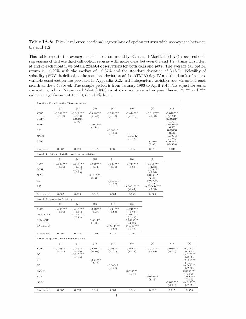
Table IA.8: Firm-level cross-sectional regressions of option returns with moneyness between0.8 and 1.2

This table reports the average coefficients from monthly Fama and MacBeth (1973) cross-sectionalregressions of delta-hedged call option returns with moneyness between 0.8 and 1.2. Using this filter,at end of each month, we obtain 224,504 observations for both calls and puts. The average call optionreturn is −0.29% with the median of −0.37% and the standard deviation of 3.18%. Volatility ofvolatility (VOV) is defined as the standard deviation of the ATM 30-day IV and the details of controlvariable construction are provided in Appendix A.2. All independent variables are winsorized eachmonth at the 0.5% level. The sample period is from January 1996 to April 2016. To adjust for serialcorrelation, robust Newey and West (1987) t-statistics are reported in parentheses. *, ** and ***indicates significance at the 10, 5 and 1% level.

Panel A: Firm-Specific Characteristics

(1) (2) (3) (4) (5) (6) (7)

VOV -0.018*** -0.019*** -0.018*** -0.018*** -0.018*** -0.018*** -0.018***(-6.30) (-6.96) (-6.48) (-6.03) (-6.16) (-6.08) (-6.91)

BETA 0.00024 0.00023*(1.52) (1.71)

SIZE 0.0011*** 0.0010***(5.88) (6.37)

BM -0.00010 0.00030(-0.15) (0.53)

MOM -0.00042 -0.00043(-0.77) (-0.95)

REV 0.0014 -0.000026(1.06) (-0.020)

R-squared 0.005 0.010 0.015 0.009 0.012 0.010 0.031

Panel B: Return Distribution Characteristics

(1) (2) (3) (4) (5) (6)

VOV -0.018*** -0.014*** -0.019*** -0.018*** -0.016*** -0.014***(-6.30) (-4.91) (-7.14) (-5.91) (-4.93) (-4.68)

IVOL -0.070*** -0.071***(-3.89) (-3.86)

MAX 0.0027** 0.0033**(2.22) (2.36)

RS -0.000065 0.000020(-0.57) (0.18)

RK -0.00010*** -0.000086***(-4.64) (-3.68)

R-squared 0.005 0.014 0.010 0.007 0.009 0.024

Panel C: Limits to Arbitrage

(1) (2) (3) (4) (5)

VOV -0.018*** -0.018*** -0.018*** -0.019*** -0.019***(-6.30) (-6.37) (-6.27) (-6.88) (-6.91)

DEMAND -0.018*** -0.013***(-6.82) (-5.44)

BID ASK 0.0011* 0.0024***(1.76) (3.49)

LN ILLIQ -0.0011*** -0.0010***(-5.89) (-5.44)

R-squared 0.005 0.010 0.008 0.016 0.024

Panel D:Option-based Characteristics

(1) (2) (3) (4) (5) (6) (7) (8)

VOV -0.018*** -0.013*** -0.020*** -0.018*** -0.026*** -0.014*** -0.019*** -0.022***(-6.30) (-5.43) (-7.69) (-6.67) (-8.71) (-5.73) (-7.75) (-11.5)

IV -0.015*** -0.013***(-8.95) (-8.63)

IS -0.024*** -0.025***(-8.79) (-10.3)

IK -0.00049 -0.0041**(-0.26) (-2.35)

RV IV 0.012*** 0.0086***(10.7) (6.32)

VTS 0.039*** 0.0087**(8.33) (2.32)

dCIV -0.022*** -0.012***(-12.6) (-7.59)

R-squared 0.005 0.029 0.012 0.007 0.014 0.016 0.015 0.056

9

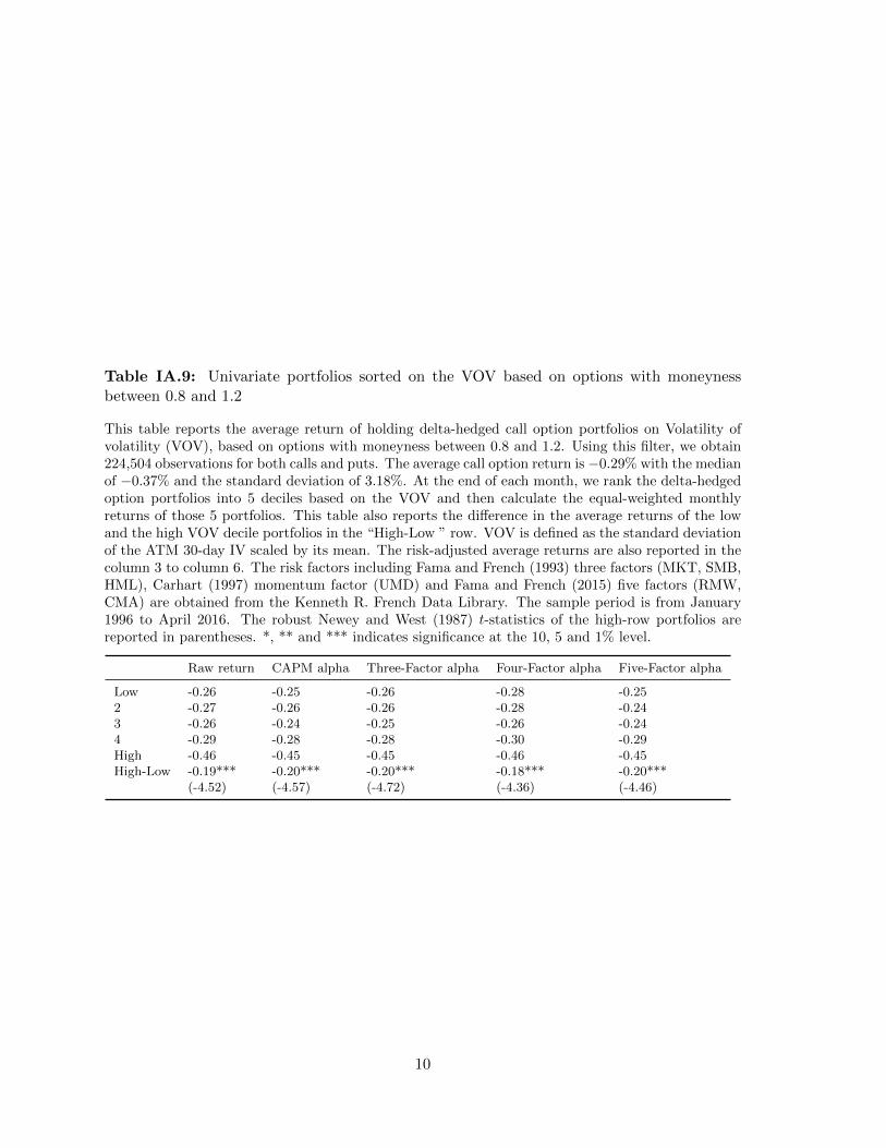
Table IA.9: Univariate portfolios sorted on the VOV based on options with moneynessbetween 0.8 and 1.2

This table reports the average return of holding delta-hedged call option portfolios on Volatility ofvolatility (VOV), based on options with moneyness between 0.8 and 1.2. Using this filter, we obtain224,504 observations for both calls and puts. The average call option return is −0.29% with the medianof −0.37% and the standard deviation of 3.18%. At the end of each month, we rank the delta-hedgedoption portfolios into 5 deciles based on the VOV and then calculate the equal-weighted monthlyreturns of those 5 portfolios. This table also reports the difference in the average returns of the lowand the high VOV decile portfolios in the “High-Low ” row. VOV is defined as the standard deviationof the ATM 30-day IV scaled by its mean. The risk-adjusted average returns are also reported in thecolumn 3 to column 6. The risk factors including Fama and French (1993) three factors (MKT, SMB,HML), Carhart (1997) momentum factor (UMD) and Fama and French (2015) five factors (RMW,CMA) are obtained from the Kenneth R. French Data Library. The sample period is from January1996 to April 2016. The robust Newey and West (1987) t-statistics of the high-row portfolios arereported in parentheses. *, ** and *** indicates significance at the 10, 5 and 1% level.

Raw return CAPM alpha Three-Factor alpha Four-Factor alpha Five-Factor alpha

Low -0.26 -0.25 -0.26 -0.28 -0.252 -0.27 -0.26 -0.26 -0.28 -0.243 -0.26 -0.24 -0.25 -0.26 -0.244 -0.29 -0.28 -0.28 -0.30 -0.29High -0.46 -0.45 -0.45 -0.46 -0.45High-Low -0.19*** -0.20*** -0.20*** -0.18*** -0.20***

(-4.52) (-4.57) (-4.72) (-4.36) (-4.46)

10

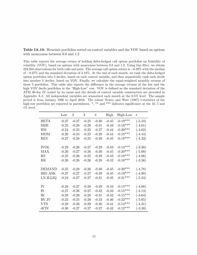
Table IA.10: Bivariate portfolios sorted on control variables and the VOV based on optionswith moneyness between 0.8 and 1.2

This table reports the average return of holding delta-hedged call option portfolios on Volatility ofvolatility (VOV), based on options with moneyness between 0.8 and 1.2. Using this filter, we obtain224,504 observations for both calls and puts. The average call option return is −0.29% with the medianof −0.37% and the standard deviation of 3.18%. At the end of each month, we rank the delta-hedgedoption portfolios into 5 deciles, based on each control variable, and then sequentially rank each decileinto another 5 deciles, based on VOV. Finally, we calculate the equal-weighted monthly returns ofthose 5 portfolios. This table also reports the difference in the average returns of the low and thehigh VOV decile portfolios in the “High-Low” row. VOV is defined as the standard deviation of theATM 30-day IV scaled by its mean and the details of control variable construction are provided inAppendix A.2. All independent variables are winsorized each month at the 0.5% level. The sampleperiod is from January 1996 to April 2016. The robust Newey and West (1987) t-statistics of thehigh-row portfolios are reported in parentheses. *, ** and *** indicates significance at the 10, 5 and1% level.

Low 2 3 4 High High-Low t

BETA -0.27 -0.27 -0.25 -0.30 -0.45 -0.19*** (-5.10)SIZE -0.25 -0.28 -0.28 -0.31 -0.43 -0.18*** (-4.61)BM -0.24 -0.25 -0.25 -0.27 -0.44 -0.20*** (-4.62)MOM -0.26 -0.24 -0.25 -0.28 -0.44 -0.18*** (-4.44)REV -0.27 -0.28 -0.25 -0.29 -0.45 -0.18*** (-4.33)

IVOL -0.29 -0.26 -0.27 -0.29 -0.43 -0.14*** (-3.30)MAX -0.26 -0.27 -0.26 -0.30 -0.45 -0.20*** (-5.00)RS -0.25 -0.26 -0.25 -0.29 -0.43 -0.18*** (-4.06)RK -0.26 -0.26 -0.26 -0.28 -0.42 -0.16*** (-3.56)

DEMAND -0.25 -0.28 -0.26 -0.30 -0.45 -0.20*** (-4.78)BID ASK -0.27 -0.27 -0.27 -0.29 -0.45 -0.19*** (-4.90)LN ILLIQ -0.24 -0.27 -0.27 -0.31 -0.45 -0.21*** (-5.24)

IV -0.28 -0.27 -0.28 -0.28 -0.43 -0.15*** (-4.08)IS -0.27 -0.26 -0.27 -0.32 -0.43 -0.15*** (-4.13)IK -0.28 -0.26 -0.28 -0.31 -0.42 -0.15*** (-3.64)RV IV -0.23 -0.25 -0.28 -0.33 -0.46 -0.22*** (-5.65)VTS -0.28 -0.26 -0.29 -0.30 -0.41 -0.14*** (-4.31)dCIV -0.30 -0.27 -0.27 -0.27 -0.42 -0.12*** (-3.30)

11

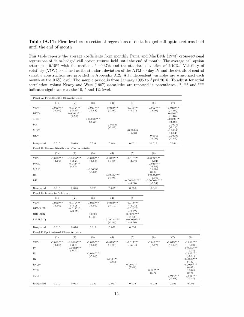
Table IA.11: Firm-level cross-sectional regressions of delta-hedged call option returns helduntil the end of month

This table reports the average coefficients from monthly Fama and MacBeth (1973) cross-sectionalregressions of delta-hedged call option returns held until the end of month. The average call optionreturn is −0.15% with the median of −0.37% and the standard deviation of 2.19%. Volatility ofvolatility (VOV) is defined as the standard deviation of the ATM 30-day IV and the details of controlvariable construction are provided in Appendix A.2. All independent variables are winsorized eachmonth at the 0.5% level. The sample period is from January 1996 to April 2016. To adjust for serialcorrelation, robust Newey and West (1987) t-statistics are reported in parentheses. *, ** and ***indicates significance at the 10, 5 and 1% level.

Panel A: Firm-Specific Characteristics

(1) (2) (3) (4) (5) (6) (7)

VOV -0.012*** -0.012*** -0.011*** -0.012*** -0.013*** -0.012*** -0.012***(-4.01) (-4.15) (-3.88) (-3.99) (-4.27) (-4.00) (-4.04)

BETA 0.00032** 0.00017(2.50) (1.40)

SIZE 0.00028*** 0.00023**(3.22) (2.48)

BM -0.00055 -0.00036(-1.48) (-1.14)

MOM -0.00045 -0.00049(-1.33) (-1.51)

REV -0.0013 -0.00094(-1.20) (-0.87)

R-squared 0.010 0.019 0.021 0.016 0.021 0.019 0.051

Panel B: Return Distribution Characteristics

(1) (2) (3) (4) (5) (6)

VOV -0.012*** -0.0095*** -0.013*** -0.012*** -0.010*** -0.0093***(-4.01) (-3.24) (-4.58) (-3.85) (-3.37) (-3.02)

IVOL -0.043*** -0.049***(-3.64) (-3.94)

MAX -0.00033 0.0010(-0.28) (0.84)

RS -0.00032*** -0.00020**(-3.05) (-2.08)

RK -0.000071*** -0.000048***(-4.80) (-3.33)

R-squared 0.010 0.026 0.020 0.017 0.018 0.048

Panel C: Limits to Arbitrage

(1) (2) (3) (4) (5)

VOV -0.012*** -0.012*** -0.013*** -0.012*** -0.014***(-4.01) (-4.08) (-4.50) (-4.10) (-4.94)

DEMAND -0.012*** -0.014***(-3.87) (-2.97)

BID ASK 0.0026 0.0075***(1.63) (4.54)

LN ILLIQ -0.00025*** -0.00039***(-2.84) (-4.26)

R-squared 0.010 0.016 0.019 0.022 0.036

Panel D:Option-based Characteristics

(1) (2) (3) (4) (5) (6) (7) (8)

VOV -0.012*** -0.0095*** -0.013*** -0.015*** -0.017*** -0.011*** -0.013*** -0.019***(-4.01) (-3.54) (-4.50) (-4.93) (-5.84) (-3.97) (-4.56) (-6.30)

IV -0.0082*** -0.0080***(-6.97) (-6.77)

IS -0.014*** -0.017***(-5.81) (-7.31)

IK 0.011*** 0.0095***(5.45) (4.32)

RV IV 0.0073*** 0.0056***(7.44) (6.07)

VTS 0.022*** 0.0028(5.77) (0.71)

dCIV -0.014*** -0.011***(-7.68) (-5.47)

R-squared 0.010 0.043 0.022 0.017 0.024 0.028 0.026 0.093

12

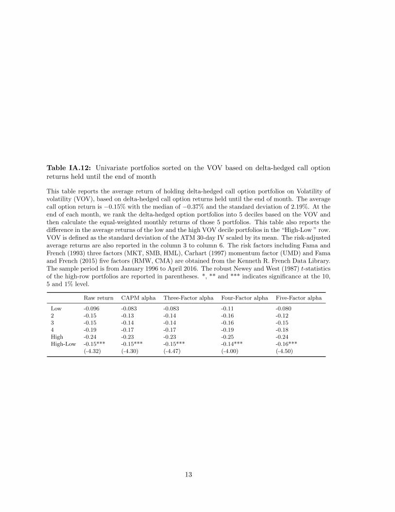
Table IA.12: Univariate portfolios sorted on the VOV based on delta-hedged call optionreturns held until the end of month

This table reports the average return of holding delta-hedged call option portfolios on Volatility ofvolatility (VOV), based on delta-hedged call option returns held until the end of month. The averagecall option return is −0.15% with the median of −0.37% and the standard deviation of 2.19%. At theend of each month, we rank the delta-hedged option portfolios into 5 deciles based on the VOV andthen calculate the equal-weighted monthly returns of those 5 portfolios. This table also reports thedifference in the average returns of the low and the high VOV decile portfolios in the “High-Low ” row.VOV is defined as the standard deviation of the ATM 30-day IV scaled by its mean. The risk-adjustedaverage returns are also reported in the column 3 to column 6. The risk factors including Fama andFrench (1993) three factors (MKT, SMB, HML), Carhart (1997) momentum factor (UMD) and Famaand French (2015) five factors (RMW, CMA) are obtained from the Kenneth R. French Data Library.The sample period is from January 1996 to April 2016. The robust Newey and West (1987) t-statisticsof the high-row portfolios are reported in parentheses. *, ** and *** indicates significance at the 10,5 and 1% level.

Raw return CAPM alpha Three-Factor alpha Four-Factor alpha Five-Factor alpha

Low -0.096 -0.083 -0.083 -0.11 -0.0802 -0.15 -0.13 -0.14 -0.16 -0.123 -0.15 -0.14 -0.14 -0.16 -0.154 -0.19 -0.17 -0.17 -0.19 -0.18High -0.24 -0.23 -0.23 -0.25 -0.24High-Low -0.15*** -0.15*** -0.15*** -0.14*** -0.16***

(-4.32) (-4.30) (-4.47) (-4.00) (-4.50)

13

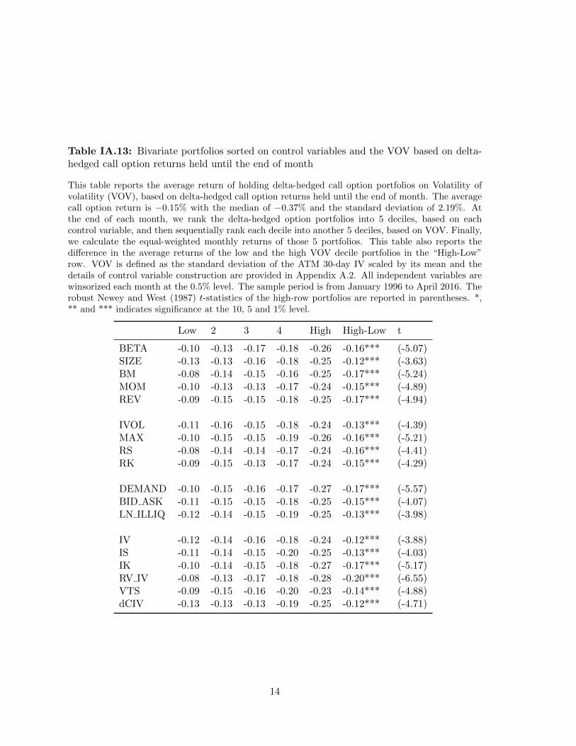
Table IA.13: Bivariate portfolios sorted on control variables and the VOV based on delta-hedged call option returns held until the end of month

This table reports the average return of holding delta-hedged call option portfolios on Volatility ofvolatility (VOV), based on delta-hedged call option returns held until the end of month. The averagecall option return is −0.15% with the median of −0.37% and the standard deviation of 2.19%. Atthe end of each month, we rank the delta-hedged option portfolios into 5 deciles, based on eachcontrol variable, and then sequentially rank each decile into another 5 deciles, based on VOV. Finally,we calculate the equal-weighted monthly returns of those 5 portfolios. This table also reports thedifference in the average returns of the low and the high VOV decile portfolios in the “High-Low”row. VOV is defined as the standard deviation of the ATM 30-day IV scaled by its mean and thedetails of control variable construction are provided in Appendix A.2. All independent variables arewinsorized each month at the 0.5% level. The sample period is from January 1996 to April 2016. Therobust Newey and West (1987) t-statistics of the high-row portfolios are reported in parentheses. *,** and *** indicates significance at the 10, 5 and 1% level.

Low 2 3 4 High High-Low t

BETA -0.10 -0.13 -0.17 -0.18 -0.26 -0.16*** (-5.07)SIZE -0.13 -0.13 -0.16 -0.18 -0.25 -0.12*** (-3.63)BM -0.08 -0.14 -0.15 -0.16 -0.25 -0.17*** (-5.24)MOM -0.10 -0.13 -0.13 -0.17 -0.24 -0.15*** (-4.89)REV -0.09 -0.15 -0.15 -0.18 -0.25 -0.17*** (-4.94)

IVOL -0.11 -0.16 -0.15 -0.18 -0.24 -0.13*** (-4.39)MAX -0.10 -0.15 -0.15 -0.19 -0.26 -0.16*** (-5.21)RS -0.08 -0.14 -0.14 -0.17 -0.24 -0.16*** (-4.41)RK -0.09 -0.15 -0.13 -0.17 -0.24 -0.15*** (-4.29)

DEMAND -0.10 -0.15 -0.16 -0.17 -0.27 -0.17*** (-5.57)BID ASK -0.11 -0.15 -0.15 -0.18 -0.25 -0.15*** (-4.07)LN ILLIQ -0.12 -0.14 -0.15 -0.19 -0.25 -0.13*** (-3.98)

IV -0.12 -0.14 -0.16 -0.18 -0.24 -0.12*** (-3.88)IS -0.11 -0.14 -0.15 -0.20 -0.25 -0.13*** (-4.03)IK -0.10 -0.14 -0.15 -0.18 -0.27 -0.17*** (-5.17)RV IV -0.08 -0.13 -0.17 -0.18 -0.28 -0.20*** (-6.55)VTS -0.09 -0.15 -0.16 -0.20 -0.23 -0.14*** (-4.88)dCIV -0.13 -0.13 -0.13 -0.19 -0.25 -0.12*** (-4.71)

14