Courtesy RK Brayton (UCB) and A Kuehlmann (Cadence) 1 Logic Synthesis Technology Mapping.

1Courtesy RK Brayton (UCB) and A Kuehlmann (Cadence)

Logic SynthesisLogic Synthesis

Technology Mapping

2

Example:t1 = a + bc;

t2 = d + e;

t3 = ab + d;

t4 = t1t2 + fg;

t5 = t4h + t2t3;

F = t5’;

This shows an unoptimized set of logic equations consisting of 16 literals

d+ea+bc

t5’

t1t2 + fg

F

ab+d

t4h + t2t3

Technology MappingTechnology Mapping

3

Optimized EquationsOptimized Equations

Using technology independent optimization, these equations are optimized using only 14 literals:

t1 = d + e;

t2 = b + h;

t3 = at2 + c;

t4 = t1t3 + fgh;

F = t4’;

d+e b+h

t4’

at2 +c

t1t3 + fgh

F

d+ea+bc

t5’

t1t2 + fg

F

ab+d

t4h + t2t3

4

Optimized EquationsOptimized Equations

Implement this network using a set of gates which form a library. Each gate has a cost (i.e. its area, delay, etc.)

5

Technology MappingTechnology Mapping

Two approaches:

• Rule-Based [LSS]

• Algoritmic [DAGON, MISII]

• Represent each function of a network using a set of base functions. This representation is called the subject graph.

• Typically the base is 2-input NANDs and inverters [MISII].

• The set should be functionally complete.

– Each gate of the library is likewise represented using the base set. This generates pattern graphs

• Represent each gate in all possible ways

6

Subject graphSubject graph

d+e b+h

t4’

at2 +c

t1t3 + fgh

b’ h’

a

d’ e’hg

f

c

Subjectgraph of2-input NANDs andinvertors

FF

7

Algorithmic ApproachAlgorithmic Approach

A cover is a collection of pattern graphs such that

• every node of the subject graph is contained in one (or more) pattern graphs

• each input required by a pattern graph is actually an output of some other graph (i.e. the inputs of one gate must exists as outputs of other gates.)

For minimum area, the cost of the cover is the sum of the areas of the gates in the cover.

Technology mapping problem: Find a minimum cost covering of the subject graph by choosing from the collection of pattern graphs for all the gates in the library.

8

Subject GraphSubject Graph

t1 = d + e;

t2 = b + h;

t3 = at2 + c;

t4 = t1t3 + fgh;

F = t4’;

F

f

g

d

e

h

b

a

c

9

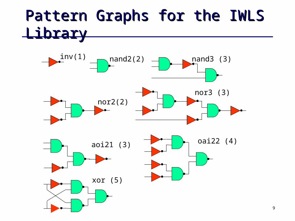
Pattern Graphs for the IWLS LibraryPattern Graphs for the IWLS Library

inv(1) nand3 (3)

oai22 (4)

nor2(2)nor3 (3)

xor (5)

aoi21 (3)

nand2(2)

10

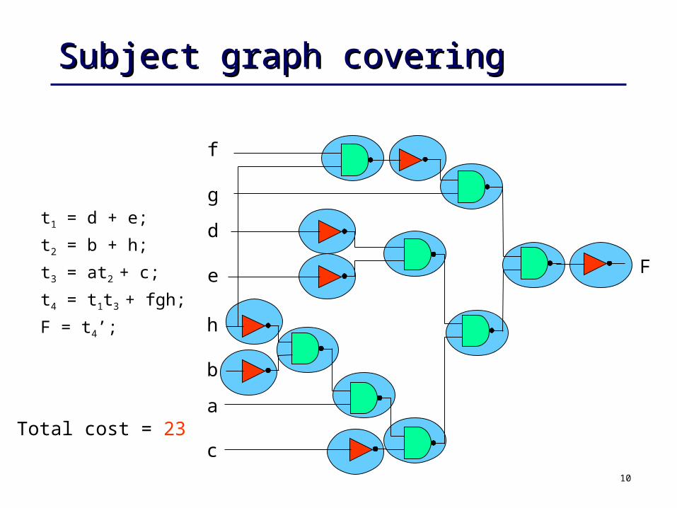
Subject graph coveringSubject graph covering

t1 = d + e;

t2 = b + h;

t3 = at2 + c;

t4 = t1t3 + fgh;

F = t4’;

F

f

g

d

e

h

b

a

cTotal cost = 23

11

Better CoveringBetter Covering

t1 = d + e;

t2 = b + h;

t3 = at2 + c;

t4 = t1t3 + fgh;

F = t4’;

F

f

g

d

e

h

b

a

c

aoi22(4)

and2(3)

or2(3)

or2(3)

Total area = 19 nand2(2)

nand2(2)

inv(1)

12

Alternate CoveringAlternate Covering

t1 = d + e;

t2 = b + h;

t3 = at2 + c;

t4 = t1t3 + fgh;

F = t4’;

F

f

g

d

e

h

b

a

c

nand3(3)nand3(3)

oai21(3)oai21(3)

oai21 (3)oai21 (3)

Total area = 15

and2(3)

inv(1)

nand2(2)

13

Tech. mapping using DAG coveringTech. mapping using DAG covering

Input:

– Technology independent, optimized logic network

– Description of the gates in the library with their cost

Output:

– Netlist of gates (from library) which minimizes total cost

General Approach:

– Construct a subject DAG for the network

– Represent each gate in the target library by pattern DAG’s

– Find an optimal-cost covering of subject DAG using the collection of pattern DAG’s

14

Tech. mapping using DAG coveringTech. mapping using DAG covering

Complexity of DAG covering:

– NP-hard

– Remains NP-hard even when the nodes have out degree 2

– If subject DAG and pattern DAG’s are trees, an efficient algorithm

exists

15

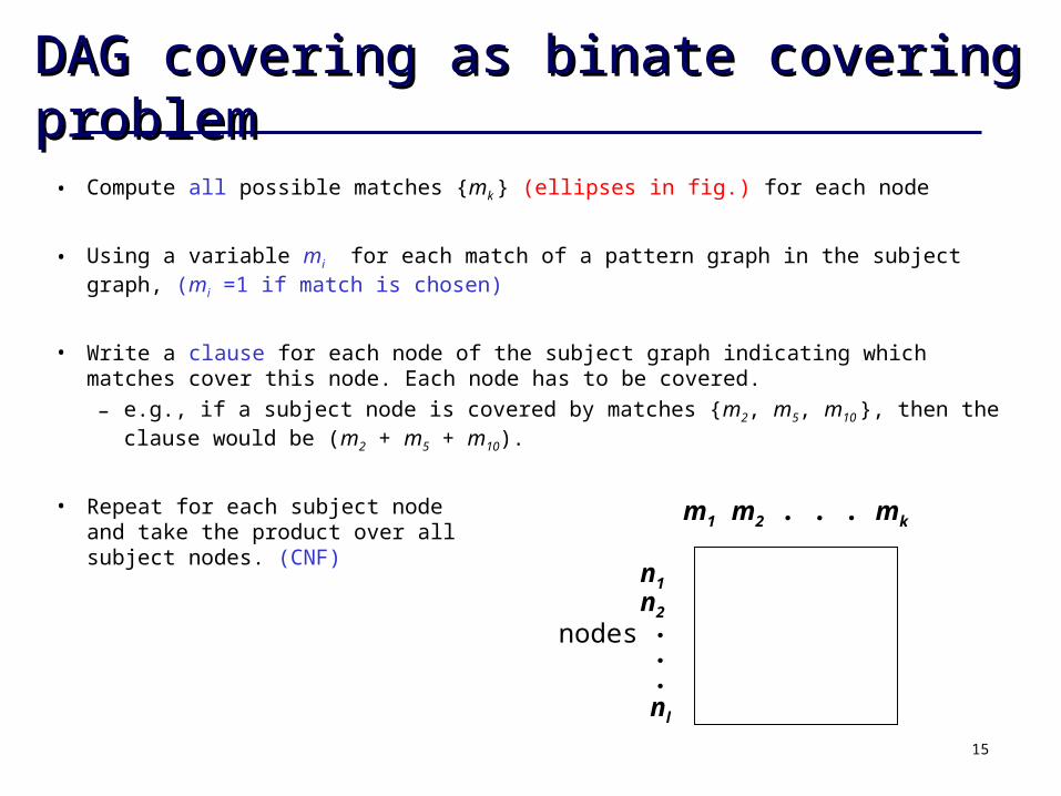
DAG covering as binate covering problemDAG covering as binate covering problem

• Compute all possible matches {mk } (ellipses in fig.) for each node

• Using a variable mi for each match of a pattern graph in the subject graph, (mi =1 if match is chosen)

• Write a clause for each node of the subject graph indicating which matches cover this node. Each node has to be covered.

– e.g., if a subject node is covered by matches {m2, m5, m10 }, then the clause would be (m2 + m5 + m10).

• Repeat for each subject node and take the product over all subject nodes. (CNF)

m1 m2 . . . mk

n1 n2 ...nl

nodes

16


Any satisfying assignment guarantees that all subject nodes are covered, but does not guarantee that other matches chosen create outputs needed as inputs needed for a given match.

Rectify this by adding additional clauses.not an outputof a chosen match

17


• Let match mi have subject nodes si1,…,sin as n inputs. If mi is chosen, one of the matches that realizes sij must also be chosen for each input j ( j not a primary input).

• Let Sij be the disjunctive expression in the variables mk giving the possible matches which realize sij as an output node. Selecting match mi implies satisfying each of the expressions Sij for j = 1 … n.This can be written

(mi (Si1 … Sin ) ) (mi + (Si1 … Sin ) ) ((mi + Si1) … (mi + Sin ) )

18


• Also, one of the matches for each primary output of the circuit must be selected.

• An assignment of values to variables mi that satisfies the above covering expression is a legal graph cover

• For area optimization, each match mi has a cost ci that is the area of the gate the match represents.

• The goal is a satisfying assignment with the least total cost.

– Find a least-cost prime:

• if a variable mi = 0 its cost is 0, else its cost in ci

• mi = 0 means that match i is not chosen

19

Binate CoveringBinate Covering

This problem is more general than unate-covering for two-level minimization because

– variables are present in the covering expression in both their true and complemented forms.

The covering expression is a binate logic function, and the problem is referred to as the binate-covering problem.

20

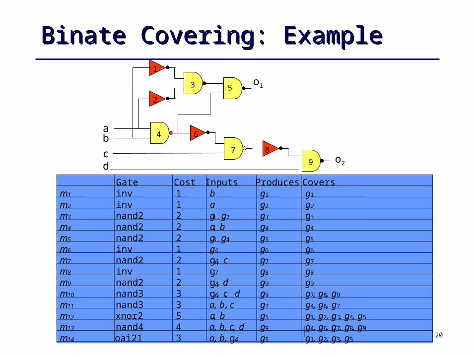
Binate Covering: ExampleBinate Covering: Example

Gate Cost Inputs Produces Covers m1 inv 1 b g1 g1 m2 inv 1 a g2 g2 m3 nand2 2 g1, g2 g3 g3 m4 nand2 2 a, b g4 g4 m5 nand2 2 g3, g4 g5 g5 m6 inv 1 g4 g6 g6 m7 nand2 2 g6, c g7 g7 m8 inv 1 g7 g8 g8 m9 nand2 2 g8, d g9 g9 m10 nand3 3 g6, c, d g9 g7, g8, g9 m11 nand3 3 a, b , c g7 g4, g6, g7 m12 xnor2 5 a, b g5 g1, g2, g3, g4, g5 m13 nand4 4 a, b, c , d g9 g4, g6, g7, g8, g9 m14 oai21 3 a, b, g4 g5 g1, g2, g3, g5

1

2

3

4

5

6

7 8

9

ab

cd

o1

o2

21


Generate constraints that each node gi be covered by some match.(m1 + m12 + m14) (m2 + m12 + m14) (m3 + m12 + m14)(m4 + m11 + m12 + m13) (m5 + m12 + m13)(m6 + m11 + m13) (m7 + m10 + m11 + m13)(m8 + m10 + m13) (m9 + m10 + m13)

To ensure that a cover leads to a valid circuit, extra clauses are generated.

– For example, selecting m3 requires that

• a match be chosen which produces g2 as an output, and

• a match be chosen which produces g1 as an output.

The only match which produces g1 is m1, and the only match which produces g2 is m2

22


The primary output nodes g5 and g9 must be realized as an output of some match.

– The matches which realize g5 as an output are m5, m12, m14;

– The matches which realize g9 as an output are m9, m10, m13

• Note:

– A match which requires a primary input as an input is satisfied trivially.

– Matches m1,m2,m4,m11,m12,m13 are driven only by primary inputs and do not require additional clauses

23


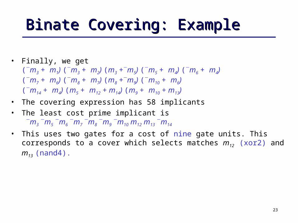
• Finally, we get(m3 + m1) (m3 + m2) (m3 +m5) (m5 + m4) (m6 + m4)(m7 + m6) (m8 + m7) (m8 +m9) (m10 + m6)(m14 + m4) (m5 + m12 + m14) (m9 + m10 + m13)

• The covering expression has 58 implicants

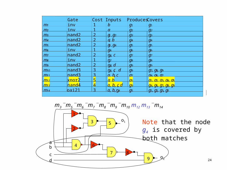
• The least cost prime implicant is m3 m5 m6 m7 m8 m9 m10 m12 m13 m14

• This uses two gates for a cost of nine gate units. This corresponds to a cover which selects matches m12 (xor2) and m13 (nand4).

24

1

2

3

4

5

6

7 89

ab

cd

o1

o2

Gate Cost Inputs Produces Covers m1 inv 1 b g1 g1 m2 inv 1 a g2 g2 m3 nand2 2 g1, g2 g3 g3 m4 nand2 2 a, b g4 g4 m5 nand2 2 g3, g4 g5 g5 m6 inv 1 g4 g6 g6 m7 nand2 2 g6, c g7 g7 m8 inv 1 g7 g8 g8 m9 nand2 2 g8, d g9 g9 m10 nand3 3 g6, c, d g9 g7, g8, g9 m11 nand3 3 a, b, c g7 g4, g6, g7 m12 xnor2 5 a, b g5 g1, g2, g3, g4, g5 m13 nand4 4 a, b, c, d g9 g4, g6, g7, g8, g9 m14 oai21 3 a, b, g4 g5 g1, g2, g3, g5

m3 m5 m6 m7 m8 m9 m10 m12 m13 m14

Note that the node g4 is covered by both matches

25

Complexity of DAG coveringComplexity of DAG covering

More general than unate covering

– Finding least cost prime of a binate function.

• Even finding a feasible solution is NP-complete (SAT).

• For unate covering, finding a feasible solution is easy.

– DAG-covering: covering + implication constraints

Given a subject graph, the binate covering provides the exact solution to the technology-mapping problem.

– However, better results may be obtained with a different initial decomposition into 2-input NANDS and inverters

Methods to solve the binate covering formulation:

– Branch and bound [Thelen]

– BDD-based [Lin and Somenzi]

Even for moderate-size networks, these are expensive.

26

Optimal Tree Covering by TreesOptimal Tree Covering by Trees

• If the subject DAG and primitive DAG’s are trees, then an efficient algorithm to find the best cover exists

• Based on dynamic programming

• First proposed for optimal code generation in a compiler

27

Optimal Tree Covering by TreesOptimal Tree Covering by Trees

Partition subject graph into forest of trees

Cover each tree optimally using dynamic programming

Given:

– Subject trees (networks to be mapped)

– Forest of patterns (gate library)

• Consider a node N of a subject tree

• Recursive Assumption: for all children of N, a best cost match (which implements the node) is known

• Cost of a leaf of the tree is 0.

• Compute cost of each pattern tree which matches at N,

Cost = SUM of best costs of implementing each input of pattern

plus the cost of the pattern

• Choose least cost matching pattern for implementing N

28

Optimum Area AlgorithmOptimum Area Algorithm

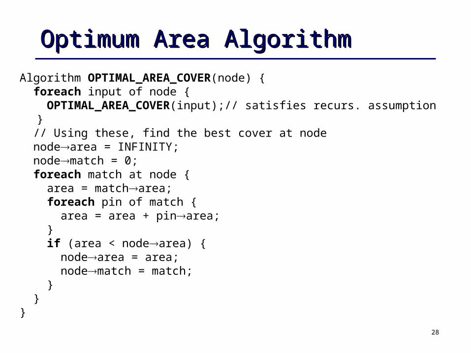
Algorithm OPTIMAL_AREA_COVER(node) { foreach input of node { OPTIMAL_AREA_COVER(input);// satisfies recurs. assumption

} // Using these, find the best cover at node nodearea = INFINITY; nodematch = 0; foreach match at node { area = matcharea; foreach pin of match { area = area + pinarea; } if (area < nodearea) { nodearea = area; nodematch = match; } }}

29

Tree Covering in ActionTree Covering in Action

nand2(3)

inv(2)

nand2(8)nand2(13)

inv(2)

nand2(3)inv(5)

and2(4)

inv(6)and2(8)

nand2(7)nand3(4)

nand2(21)nand3(22)nand4(18)

inv(20)aoi21(18)

nand2(21)nand3(23)nand4(22)

nand2 = 3inv = 2nand3 = 4nand4 = 5and2 = 4aio21 = 4oai21 = 4

Library:

nand4nand4

aoi21aoi21

nand4nand4

30

Complexity of Tree CoveringComplexity of Tree Covering• Complexity is controlled by finding all sub-trees of the subject graph

which are isomorphic to a pattern tree.

• Linear complexity in both size of subject tree and size of collection of pattern trees

31

Partitioning the Subject DAG into TreesPartitioning the Subject DAG into Trees

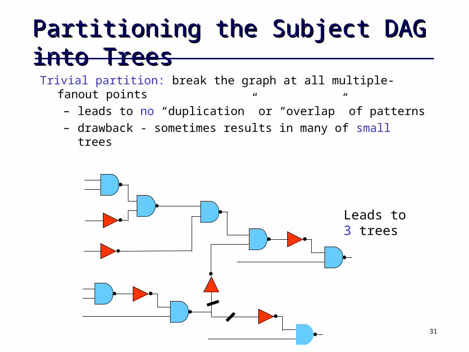
Trivial partition: break the graph at all multiple-fanout points

– leads to no “duplication” or “overlap” of patterns

– drawback - sometimes results in many of small trees

Leads to 3 trees

32

Partitioning the subject DAG into treesPartitioning the subject DAG into treesSingle-cone partition:

– from a single output, form a large tree back to the primary inputs; – map successive outputs until they hit match output formed from mapping

previous primary outputs.• Duplicates some logic (where trees overlap)• Produces much larger trees, potentially better area results

output

output

33

Min-Delay CoveringMin-Delay Covering

• For trees:– identical to min-area covering

– use optimal delay values within the dynamic programming paradigm

• For DAGs:– if delay does not depend on number of fanouts: use dynamic

programming as presented for trees

– leads to optimal solution in polynomial time

• “we don’t care if we have to replicate logic”

• Combined objective– e.g. apply delay as first criteria, then area as second

– combine with static timing analysis to focus on critical paths

34

Combined Decomposition and Technology Mapping Combined Decomposition and Technology Mapping

Common Approach:

• Phase 1: Technology independent optimization

– commit to a particular Boolean network

– algebraic decomposition used

• Phase 2: AND2/INV decomposition

– commit to a particular decomposition of a general Boolean network using 2-input ANDs and inverters

• Phase 3: Technology mapping (tree-mapping)

35

Drawbacks:

Procedures in each phase are disconnected:

– Phase 1 and Phase 2 make critical decisions without knowing much about constraints and library

– Phase 3 knows about constraints and library, but solution space is restricted by decisions made earlier


36

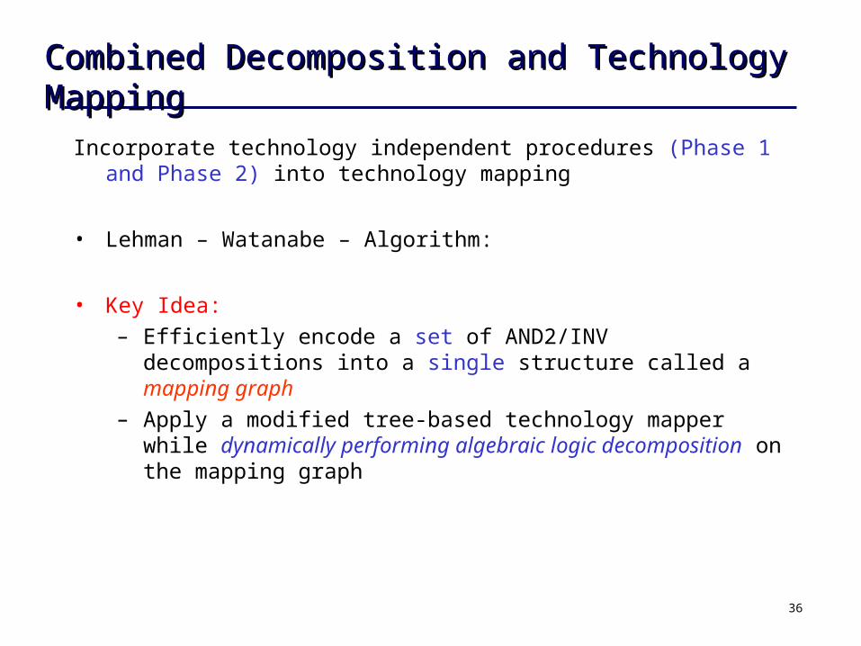
Incorporate technology independent procedures (Phase 1 and Phase 2) into technology mapping

• Lehman – Watanabe – Algorithm:

• Key Idea:

– Efficiently encode a set of AND2/INV decompositions into a single structure called a mapping graph

– Apply a modified tree-based technology mapper while dynamically performing algebraic logic decomposition on the mapping graph


37

OutlineOutline

• Mapping Graph– Encodes a set of AND2/INV decompositions

• Tree-mapping on a mapping graph: graph-mapping -mapping:

– without dynamic logic decomposition– solution space: Phase 3 + Phase 2

-mapping:– with dynamic logic decomposition– solution space: Phase 3 + Phase 2 + Algebraic decomposition (Phase 1)

• Experimental results

38

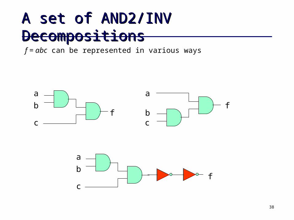
A set of AND2/INV DecompositionsA set of AND2/INV Decompositions

f = abc can be represented in various ways

f

a

b

c

a

b

c

a

bc

f

f

39

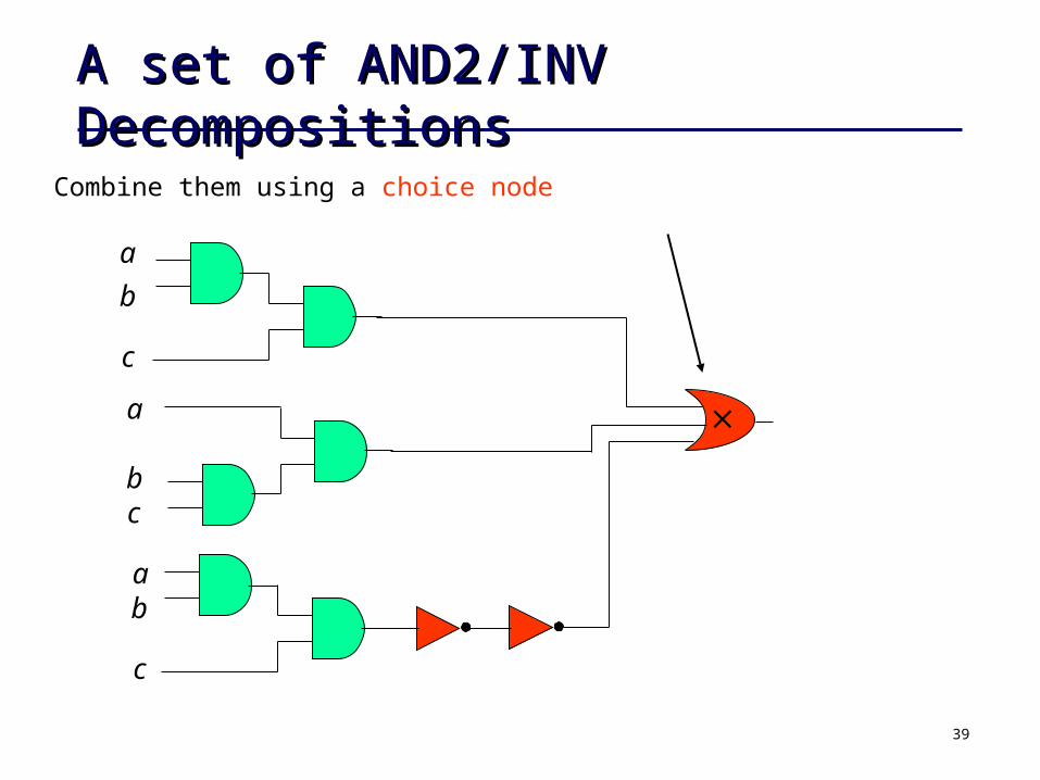
Combine them using a choice node

a

b

c

ab

c

a

bc


40

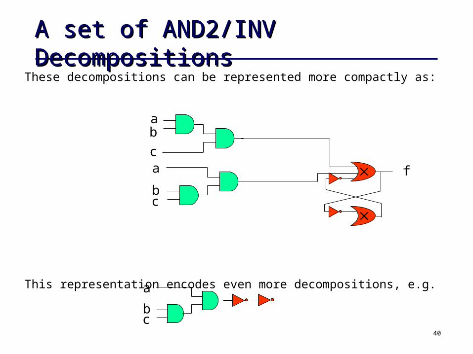
These decompositions can be represented more compactly as:

This representation encodes even more decompositions, e.g.

ab

ca

bc

f

bc

a


41

Mapping GraphMapping Graph

A Boolean network containing 4 modifications:

– Choice node: choices on different decompositions

– Cyclic: functions written in terms of each other, e.g. inverter chain with an arbitrary length

– Reduced: No two choice nodes with same function. No two AND2s with same fanin. (like BDD node sharing)

– Ugates: just for efficient implementation - do not explicitly represent choice nodes and inverters

For CHT benchmark (MCNC’91), there are 2.2x1093 AND2/INV decompositions. All are encoded with only 400 ugates containing 599 AND2s in total.

bc

a

bc

a

ab

bc

ac

abc

ugates

42

Tree-mapping on a Mapping GraphTree-mapping on a Mapping Graph

Graph-Mapping on Trees**: Apply dynamic program-

ming from primary inputs:– find matches at each AND2

and INV, and – retain the cost of a best

cover at each node• a match may contain choice nodes• the cost at a choice node is the

minimum of fanin costs• fixed-point iteration on each cycle,

until costs of all the nodes in the cycle become stable

Run-time is typically linear in the size of the mapping graph

** mapping graph may not be a tree, but any multiple fanout node just represents several copies of same function.

bc

a

bc

a

ab

bc

ac

abc

AND3

43

Example: Tree-mappingExample: Tree-mapping

Delay: best choice if c is later than a and b.

subject graph library pattern graph

44

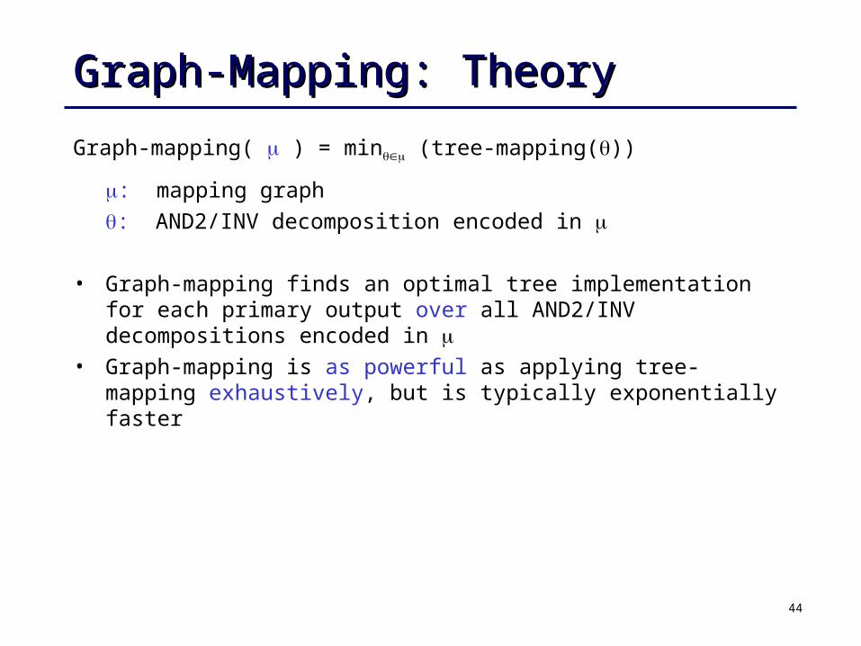
Graph-Mapping: TheoryGraph-Mapping: Theory

Graph-mapping( ) = min (tree-mapping())

: mapping graph

: AND2/INV decomposition encoded in

• Graph-mapping finds an optimal tree implementation for each primary output over all AND2/INV decompositions encoded in

• Graph-mapping is as powerful as applying tree-mapping exhaustively, but is typically exponentially faster

45

-Mapping-Mapping

Given a Boolean network ,

• Generate a mapping graph :

• For each node of ,

• encode all AND2 decompositions for each product termExample: abc 3 AND2 decompositions: a(bc), c(ab), b(ca)

• encode all AND2/INV decompositions for the sum termExample: p+q+r 3 AND2/INV decompositions:

p+(q+r), r+(p+q), q+(r+p).

• Apply graph-mapping on

In practice, is pre-processed so

• each node has at most 10 product terms and

• each term has at most 10 literals

46

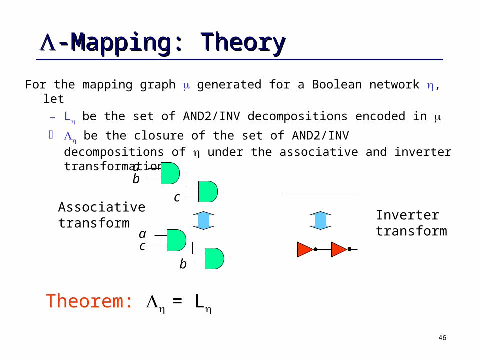
-Mapping: Theory-Mapping: Theory

For the mapping graph generated for a Boolean network , let

– L be the set of AND2/INV decompositions encoded in be the closure of the set of AND2/INV decompositions of under the

associative and inverter transformations:

ab

c

ac

b

Associativetransform

Invertertransform

Theorem: = L

47

Dynamic Logic DecompositionDynamic Logic Decomposition

During graph-mapping, dynamically modify the mapping graph:

find D-patterns and add F-patterns

D-pattern: acab

a

b ab

cc

F-pattern: )( cba

48

Dynamic Logic DecompositionDynamic Logic Decomposition

Note: Adding F-patterns may introduce new D-patterns which may imply new F-patterns.

ab

c

ab

c

b

c

ac

a

abc

b

49

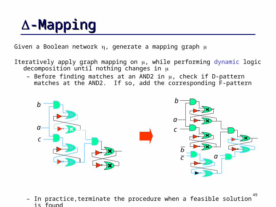
-Mapping-Mapping

Given a Boolean network , generate a mapping graph

Iteratively apply graph mapping on , while performing dynamic logic decomposition until nothing changes in – Before finding matches at an AND2 in , check if D-pattern matches at

the AND2. If so, add the corresponding F-pattern

– In practice,terminate the procedure when a feasible solution is found

b

c

a c

a

abc

b

50

-Mapping-Mapping

For the mapping graph generated for a Boolean network , let

– D be the set of AND2/INV decompositions encoded in the resulting mapping graph.

be the closure of under the distributive transformation:

Theorem: = D

a

abb

cc

51

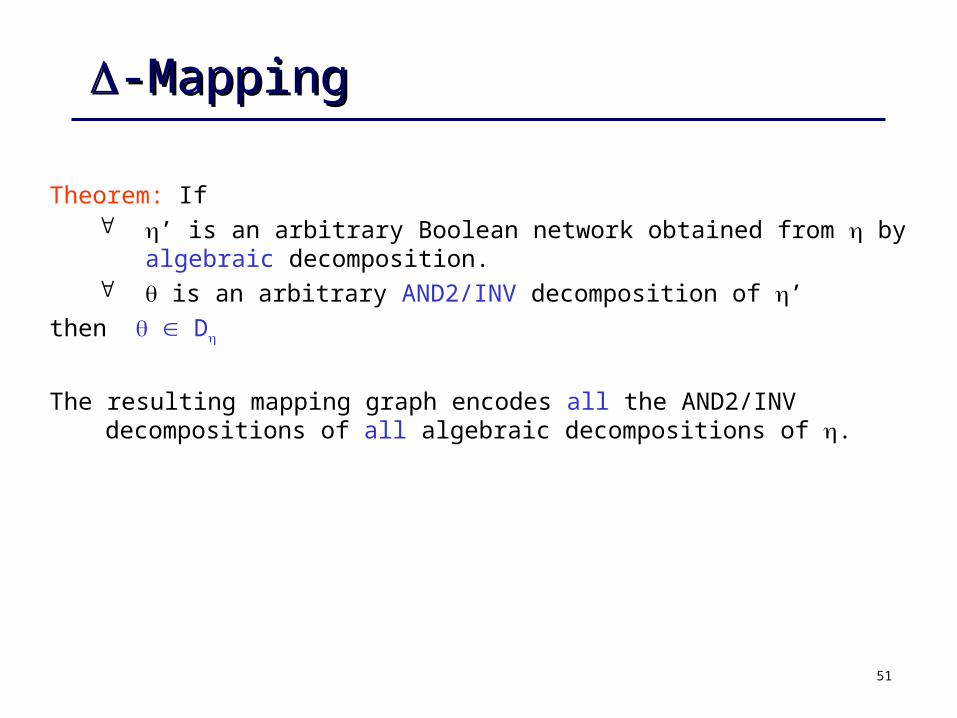
-Mapping-Mapping

Theorem: If ’ is an arbitrary Boolean network obtained from by algebraic

decomposition. is an arbitrary AND2/INV decomposition of ’

then D

The resulting mapping graph encodes all the AND2/INV decompositions of all algebraic decompositions of .

52

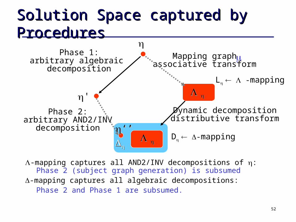
Solution Space captured by ProceduresSolution Space captured by Procedures

-mapping captures all AND2/INV decompositions of : Phase 2 (subject graph generation) is subsumed

-mapping captures all algebraic decompositions: Phase 2 and Phase 1 are subsumed.

Phase 1:arbitrary algebraic

decomposition

Phase 2:arbitrary AND2/INV

decomposition

Mapping graphassociative transform

Dynamic decompositiondistributive transform

'

D -mapping

L -mapping

‘’‘’

53

SummarySummary

• Logic decomposition during technology mapping– Efficiently encode a set on AND2/INV decompositions– Dynamically perform logic decomposition

• Two mapping procedures -mapping: optimal over all AND2/INV decompositions (associative rule) -mapping: optimal over all algebraic decompositions (distributive rule)

• Was implemented and used for commercial design projects (in DEC/Compac alpha)

• Extended for sequential circuits:– considers all retiming possibilities (implicitly) and algebraic factors across

latches

Courtesy RK Brayton (UCB) and A Kuehlmann (Cadence) 1 Logic Synthesis Technology Mapping.

Documents

Transcript of Courtesy RK Brayton (UCB) and A Kuehlmann (Cadence) 1 Logic Synthesis Technology Mapping.