DEPARTMENT OF ELECTRICAL AND

ELECTRONICS ENGINEERING

COURSE MATERIAL

EE8391 - ELECTRICTROMAGNETIC THEORY

II YEAR- III SEMESTER

DEPARTMENT OF ELECTRICAL AND ELECTRONICS ENGINEERING (SYLLABUS)

Sub. Code : EE8391 Branch/Year/Sem : EEE/IV/VIII

Sub Name : ELECTRICTROMAGNETIC THEORY Staff Name : S.BALAMURUGAN

UNIT I ELECTROSTATICS – I 9

Sources and effects of electromagnetic fields – Coordinate Systems – Vector fields – Gradient,

Divergence, Curl – theorems and applications – Coulomb‟s Law – Electric field intensity – Field due

to discrete and continuous charges – Gauss‟s law and applications.

UNIT II ELECTROSTATICS – II 9 Electric potential – Electric field and Equipotential plots, Uniform and Non-Uniform field,

Utilization factor – Electric field in free space, conductors, dielectrics - Dielectric polarization –

Dielectric strength - Electric field in multiple dielectrics – Boundary conditions, Poisson‟s and

Laplace‟s equations, Capacitance, Energy density, Applications.

UNIT III MAGNETOSTATICS 9 Lorentz force, magnetic field intensity (H) – Biot–Savart‟s Law – Ampere‟s Circuit Law – H

due to straight conductors, circular loop, infinite sheet of current, Magnetic flux density (B) – B in

free space, conductor, magnetic materials – Magnetization, Magnetic field in multiple media –

Boundary conditions, scalar and vector potential, Poisson‟s Equation, Magnetic force, Torque,

Inductance, Energy density, Applications.

UNIT IV ELECTRODYNAMIC FIELDS 9 Magnetic Circuits – Faraday‟s law – Transformer and motional EMF – Displacement current

– Maxwell‟s equations (differential and integral form) – Relation between field theory and circuit theory – Applications.

UNIT V ELECTROMAGNETIC WAVES 9 Electromagnetic wave generation and equations – Wave parameters; velocity, intrinsic

impedance, propagation constant – Waves in free space, lossy and lossless dielectrics, conductors-

skin depth - Poynting vector – Plane wave reflection and refraction – Standing Wave – Applications. TOTAL (L:45+T:15):

EE8391-ELCTROMAGNETIC THEORY

OUTCOMES: Ability to understand and apply basic science, circuit theory, Electro-magnetic field theory

control theory and apply them to electrical engineering problems.

TEXT BOOKS: 1. Mathew N. O. Sadiku, „Principles of Electromagnetics‟, 4 th Edition ,Oxford University Press Inc. First India edition, 2009. 2. Ashutosh Pramanik, „Electromagnetism – Theory and Applications‟, PHI Learning Private Limited, New Delhi, Second Edition-2009. 3. K.A. Gangadhar, P.M. Ramanthan „ Electromagnetic Field Theory (including Antennaes and wave

propagation‟, 16th Edition, Khanna Publications, 2007.

REFERENCES: 1. Joseph. A.Edminister, „Schaum‟s Outline of Electromagnetics, Third Edition (Schaum‟s Outline Series), Tata McGraw Hill, 2010 2. William H. Hayt and John A. Buck, „Engineering Electromagnetics‟, Tata McGraw Hill 8

th

Revised edition, 2011. 3. Kraus and Fleish, „Electromagnetics with Applications‟, McGraw Hill International Editions, Fifth Edition, 2010. 4. Bhag Singh Guru and Hüseyin R. Hiziroglu “Electromagnetic field theory Fundamentals”, Cambridge University Press; Second Revised Edition, 2009. Prepared by Verified By S.BALAMURUGAN HOD

Approved by PRINCIPAL

UNIT 1

INTRODUCTION

1.1Introduction

Electromagnetic theory is a discipline concerned with the study of charges at rest and in motion.

Electromagnetic principles are fundamental to the study of electrical engineering and physics. is also

indispensable to the understanding, analysis and design of various electrical, electromechanical and

electronic systems. Some of the branches of study where

Electromagnetic principles find applications are:

1. RF communication 2. Microwave Engineering 3. Antennas 4. Electrical Machines 5. Satellite Communication 6. Atomic and nuclear research 7. Radar Technology 8. Remote sensing 9. EMI EMC 10. Quantum Electronics 11. VLSI

is a prerequisite for a wide spectrum of studies in the field of Electrical Sciences and Physics. can be

thought of as generalization of circuit theory. There are certain situations that can be handled exclusively in

terms of field theory. In , the quantities involved can be categorized as source quantities and field

quantities. Source of electromagnetic field is electric charges: either at rest or in motion. However an

electromagnetic field may cause a redistribution of charges that in turn change the field and hence the

separation of cause and effect is not always visible.

1.2. Sources and effects of electromagnetic fields

Sources of EMF: Current carrying conductors. Mobile phones. Microwave oven. Computer and Television screen. High voltage Power lines.

Effects of Electromagnetic fields: Plants and Animals. Humans. Electrical components.

Fields are classified as Scalar field Vector field.

1.3. Co-ordinate Systems

In order to describe the spatial variations of the quantities, we require using appropriate co-ordinate system. A point or vector can be represented in a curvilinear coordinate system that may be orthogonal or non-orthogonal .

An orthogonal system is one in which the co-ordinates are mutually perpendicular. Non-orthogonal co-ordinate systems are also possible, but their usage is very limited in practice In the following sections we discuss three most commonly used orthogonal co -ordinate systems, viz:

1. Cartesian (or rectangular) co-ordinate system

2. Cylindrical co-ordinate system

3. Spherical polar co-ordinate system

1.3.1 Cartesian Co-ordinate System : In Cartesian co-ordinate system, we have, (u,v,w) = (x,y,z). A point P(X0, y0, z0) in Cartesian co-ordinate system is represented as intersection of three planes X = X0, Y = Y0 and Z = Z0. The unit vectors satisfies the following relation:

In cartesian co-ordinate system, a vector can be written as . The

dot and cross product of two vectors and can be written as follows:

Since x, y and z all represent lengths, h1= h2= h3=1. The differential length, area and volume are defined respectively as

1.3.2 Cylindrical co-ordinate system:

For cylindrical coordinate systems we have a point is

determined as the point of intersection of a cylindrical surface r = r0, half plane containing the

z-axis and

making an angle ; with the xz plane and a plane parallel to XY plane located at z=z0 as

shown in figure 7 on next page.

In cylindrical coordinate system, the unit vectors satisfy the following relations

A vector can be written as ,

The differential length is defined as,

.

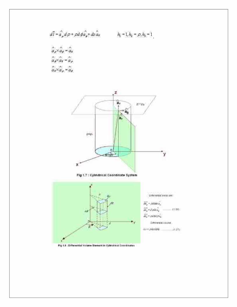
1.3.3 Transformation between Cartesian and Cylindrical coordinates:

Let us consider is to be expressed in Cartesian co-ordinate as

. In doing so we note that and

it applies for other components as well.

These relations can be put conveniently in the matrix form as:

themselves may be functions of as:

Thus we see that a vector in one coordinate system is transformed to another coordinate system through

two-step process: Finding the component vectors and then variable transformation.

Fig 1.10: Spherical Polar Coordinate System

1.3.4 Spherical Polar Coordinates:

For spherical polar coordinate system, we have, . A point

is represented as the intersection of

(i) Spherical surface r=r0

(ii) Conical surface ,and

half plane containing z-axis making angle with the xz plane as shown in the

vector in spherical polar co-ordinates is written as : and

For spherical polar coordinate system we have h1=1, h2= r and h3= .

With reference to the Figure, the elemental areas are:

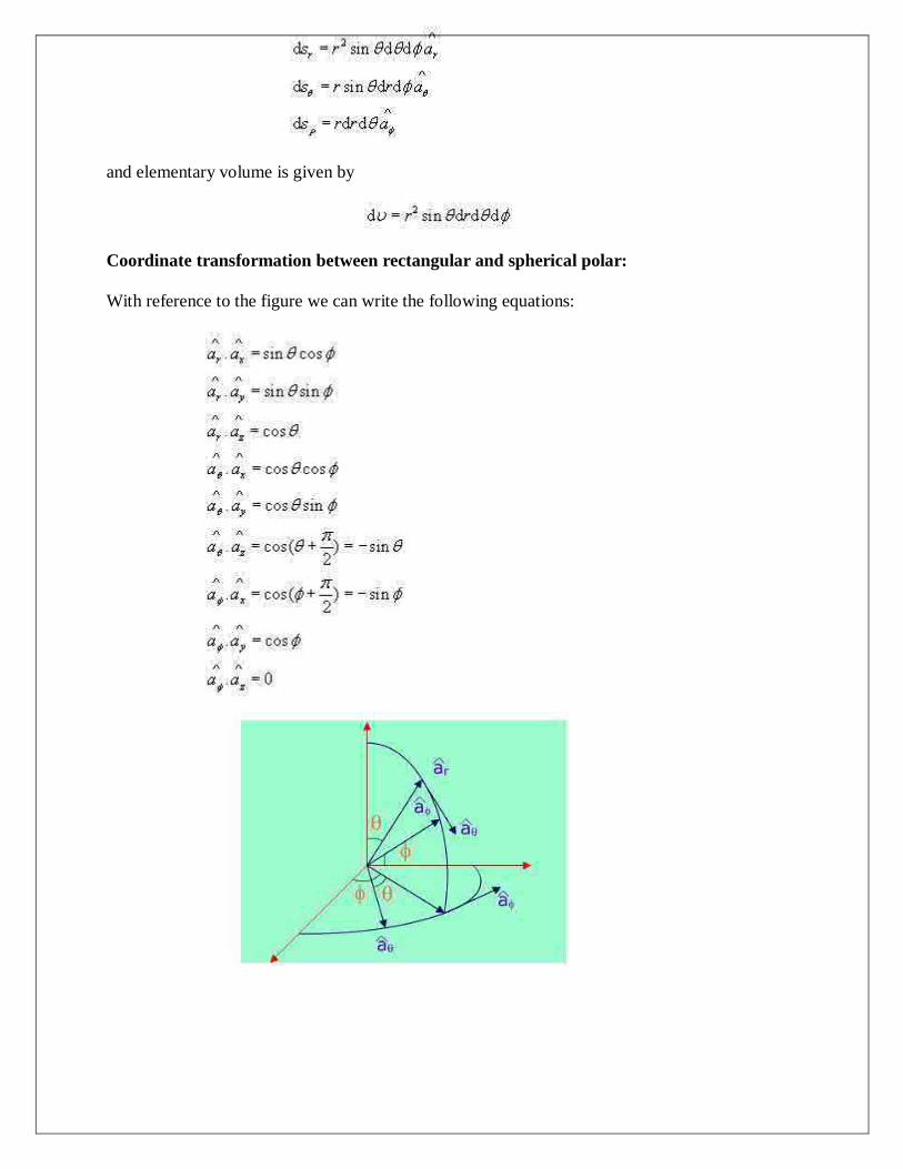
and elementary volume is given by

Coordinate transformation between rectangular and spherical polar:

With reference to the figure we can write the following equations:

Given a vector in the spherical polar coordinate system, its component in

the cartesian coordinate system can be found out as follows:

Similarly,

The above equation can be put in a compact form:

The components themselves will be functions of . are

related to x,y and z as: and conversely,

1.4 Vector Fields:

The quantities that we deal in may be either scalar or vectors [There are other class of physical

quantities called Tensors: where magnitude and direction vary with co ordinate axes]. Scalars are

quantities characterized by magnitude only and algebraic sign. A quantity that has direction as well as

magnitude is called a vector. Both scalar and vector quantities are function of time and position . A field

is a function that specifies a particular quantity everywhere in a region. Depending upon the nature of

the quantity under consideration, the field may be a vector or a scalar field. Example of scalar field is the

electric potential in a region while electric or magnetic fields at any point is the example of vector field.

1.5 Properties

Associative law.

Distributive Law

Product of Vectors

When two vectors and are multiplied, the result is either a scalar or a vector depending

how the two vectors were multiplied. The two types of vector multiplication are:

Scalar product (or dot product) gives a scalar.

Vector product (or cross product) gives a vector.

The dot product between two vectors is defined as

=|A||B| cosθAB

Vector product

is unit vector perpendicular to and

The dot product is commutative i.e., and distributive i.e.,

Associative law does not apply to scalar product.

The vector or cross product of two vectors and is denoted by

. is a vector perpendicular to the plane containing and , the magnitude is given

by 1.5.1 Gradient of a Scalar function: Let us consider a scalar field V(u,v,w) , a function of space coordinates.

Gradient of the scalar field V is a vector that represents both the magnitude and direction of the maximum space rate of increase of this scalar field V.

Gradient of a scalar function

As shown in figure let us consider two surfaces S1and S2 where the function V has constant

magnitude and the magnitude differs by a small amount dV. Now as one moves from S1 to S2, the magnitude of spatial rate of change of V i.e. dV/dl depends on the direction of elementary path length dl, the maximum occurs when one traverses from S1to S2along a path normal to the surfaces as in this case the distance is minimum.

By our definition of gradient we can write:

since which represents the distance along the normal is the shortest distance between the two

surfaces. For a general curvilinear coordinate system

Further we can write

Hence,

Also we can write,

By comparison we can write,

Hence for the Cartesian, cylindrical and spherical polar coordinate system, the expressions for Gradient can be written as: In Cartesian coordinates:

In cylindrical coordinates:

and in spherical polar coordinates:

The following relationships hold for gradient operator.

.

where U and V are scalar functions and n is an integer.

It may further be noted that since magnitude of depends on the direction of dl, it is

called the directional derivative. If is called the scalar potential function of the vector

function .

1.5.2Divergence of a Vector Field: In study of vector fields, directed line segments, also called flux lines or streamlines, represent field

variations graphically. The intensity of the field is proportional to the density of lines. For example, the

number of flux lines passing through a unit surface S normal to the vector measures the vector field

strength.

Flux Lines

We have already defined flux of a vector field as

..

For a volume enclosed by a surface,

We define the divergence of a vector field at a point P as the net outward flux from a volume

enclosing P, as the volume shrinks to zero.

Here is the volume that encloses P and S is the corresponding closed surface.

Divergence theorem : Divergence theorem states that the volume integral of the divergence of vector field is equal to the net

outward flux of the vector through the closed surface that bounds the volume. Mathematically, Proof: Let us consider a volume V enclosed by a surface S . Let us subdivide the volume in large number of

cells. Let the kth

cell has a volume and the corresponding surface is denoted by Sk. Interior to the

volume, cells have common surfaces. Outward flux through these common surfaces from one cell

becomes the inward flux for the neighboring cells. Therefore when the total flux from these cells are

considered, we actually get the net outward flux through the surface surrounding the volume. Hence we

can write:

In the limit, that is when and the right hand of the expression can be written as

Hence we get , which is the divergence theorem.

1.5.3 Curl of a vector field

We have defined the circulation of a vector field A around a closed path as .

Curl of a vector field is a measure of the vector field's tendency to rotate about a point. Curl , also

written as is defined as a vector whose magnitude is maximum of the net circulation per unit area

when the area tends to zero and its direction is the normal direction to the area when the area is oriented

in such a way so as to make the circulation maximum.

Therefore, we can write:

......................................(1.68)

To derive the expression for curl in generalized curvilinear coordinate system, we first compute

and to do so let us consider the figure

Curl of a Vector

Curl operation exhibits the following properties:

1.6. Stoke's theorem :

It states that the circulation of a vector field around a closed path is equal to the integral of

over the surface bounded by this path. It may be noted that this equality holds provided

and are continuous on the surface.

i.e,

. Proof: Let us consider an area S that is subdivided into large number of cells as shown in the figure

Stokes theorem

Let kthcell has surface area and is bounded path Lk while the total area is bounded by path L.

As seen from the figure that if we evaluate the sum of the line integrals around the elementary areas,

there is cancellation along every interior path and we are left the line integral along path L. Therefore we

can write,

As 0 .

1.6.1 Divergence theorem : Divergence theorem states that the volume integral of the divergence of vector field is equal to the net outward flux of the vector through the closed surface that bounds the volume. Mathematically,

Proof:

Let us consider a volume V enclosed by a surface S . Let us subdivide the volume in large number of

cells. Let the kth

cell has a volume and the corresponding surface is denoted by Sk. Interior to the

volume, cells have common surfaces. Outward flux through these common surfaces from one cell

becomes the inward flux for the neighboring cells. Therefore when the total flux from these cells are

considered, we actually get the net outward flux through the surface surrounding the volume. Hence we

can write:

In the limit, that is when and the right hand of the expression can be written as

. Hence we get , which is the divergence theorem.

1.6.2 Coulomb’s Law

Coulomb's Law states that the force between two point charges Q1and Q2 is directly proportional to the product of the charges and inversely proportional to the square of the distance between them.

Point charge is a hypothetical charge located at a single point in space. It is an idealised model of a particle having an electric charge.

Mathematically, ,where k is the proportionality constant.

In SI units, Q1 and Q2 are expressed in Coulombs(C) and R is in meters.

Force F is in Newtons (N) and , is called the permittivity of free space.

(We are assuming the charges are in free space. If the charges are any other

dielectric medium, we will use instead where is called the relative permittivity

or the dielectric constant of the medium).

As shown in the Figure 2.1 let the position vectors of the point charges

Q1and Q2 are given by and . Let represent the force on Q1 due to charge Q2.

The charges are separated by a distance of . We define the unit

vectors as

and

can be defined as .

Similarly the force on Q1 due to charge Q2 can be calculated and if represents this

force then we can write

When we have a number of point charges, to determine the force on a

particular charge due to all other charges, we apply principle of

superposition. If we have N number of charges Q1,Q2,.........QN located

respectively at the points represented by the position vectors , ,...... ,

the force experienced by a charge Q located at is given by,

1.6.3 Electric field intensity

Electric field intensity is the strength of an electric field at any point. It is equal to the electric

force per unit charge experienced by a test charge placed at that point. The unit of measurement is volts

per meter (V/m) or newtons per coulomb (N/C). This physical quantity has dimensions MLT−3

A−1

.

It is a vector quantity, and its direction is along the direction of force.

1.7. Field due to discrete and continuous charges

Line, surface and volume integrals

In , we come across integrals, which contain vector functions. Some representative integrals are listed below:

In the above integrals, and respectively represent vector and scalar function of space coordinates.

C,S and V represent path, surface and volume of integration. All these integrals are evaluated using extension

of the usual one-dimensional integral as the limit of a sum, i.e., if a function f(x) is defined over arrange a to b

of values of x, then the integral is given by

where the interval (a,b) is subdivided into n continuous interval of lengths .

Line Integral: Line integral is the dot product of a vector with a specified C; in other words it is

the integral of the tangential component along the curve C.

As shown in the figure 1.14, given a vector around C, we define the integral as the

line integral of E along the curve C. If the path of integration is a closed path as shown in the figure the

line integral becomes a closed line integral and is called the circulation of around C and denoted asas

shown in the figure

Surface Integral :

Given a vector field , continuous in a region containing the smooth surface S, we define the

surface integral or the flux of through S as as surface integral

over surface S.

Surface Integral If the surface integral is carried out over a closed surface, then we write

Volume Integrals:

We define or as the volume integral of the scalar function f(function of spatial

coordinates) over the volume V. Evaluation of integral of the form can be carried out as a sum of

three scalar volume integrals, where each scalar volume integral is a component of the

vector

The Del Operator :

The vector differential operator was introduced by Sir W. R. Hamilton and later on developed by P.

G. Tait.

Mathematically the vector differential operator can be written in the general form as:

In Cartesian coordinates:

In cylindrical coordinates:

and in spherical polar coordinates:

Unit II Electrostatics

2.1. Electro statics

In the previous chapter we have covered the essential mathematical tools needed to

study EM fields. We have already mentioned in the previous chapter that electric charge

is a fundamental property of matter and charge exist in integral multiple of electronic

charge. Electrostatics can be defined as the study of electric charges at rest. Electric fields

have their sources in electric charges.In this chapter we first study two fundamental laws

governing the electrostatic fields, viz, (1) Coulomb's Law and (2) Gauss's Law. Both

these law have experimental basis. Coulomb's law is applicable in finding electric field

due to any charge distribution, Gauss's law is easier to use when the distribution is

symmetrical.

Electric Field

The electric field intensity or the electric field strength at a point is defined as the force per unit charge. That is

or, The electric field intensity E at a point r (observation point) due a point charge Q located

at (source point) is given by:

For a collection of N point charges Q1 ,Q2 ,.........QN located at , ,...... ,

the electric field intensity at point is obtained as

The expression (2.6) can be modified suitably to compute the electric filed due to a continuous distribution of charges. In figure 2.2 we consider a continuous volume distribution of charge (t) in the region denoted as the source region.

For an elementary charge , i.e. considering this charge as point charge, we

can write the field expression as:

Continuous Volume Distribution of Charge When this expression is integrated over the source region, we get the electric field at the point P due to this distribution of charges. Thus the expression for the electric field at P can be written as:

Similar technique can be adopted when the charge distribution is in the form of a line charge density or a surface charge density.

2.1.1 Electric Potential

At a point in space, the electric potential is the potential energy per unit of charge that

is associated with a static (time-invariant) electric field. It is typically measured

in volts, and is a Lorentz scalar quantity. The difference in electrical potential between

two points is known as voltage.Mathematically, it is the potential φ (a scalar field)

associated with the conservative electric field ( ) that occurs when

the magnetic field is time invariant (so that

from Faraday's law of induction).

In the previous sections we have seen how the electric field intensity due to a charge

or a charge distribution can be found using Coulomb's law or Gauss's law. Since a charge

placed in the vicinity of another charge (or in other words in the field of other charge)

experiences a force, the movement of the charge represents energy exchange.

Electrostatic potential is related to the work done in carrying a charge from one point to

the other in the presence of an electric field.

Let us suppose that we wish to move a positive test charge from a point P to another

point Q as shown in the Fig. 2.8.

The force at any point along its path would cause the particle to accelerate and move it

out of the region if unconstrained. Since we are dealing with an electrostatic case, a force

equal to the negative of that acting on the charge is to be applied while moves from P

to Q. The work done by this external agent in moving the charge by a distance is

given by:

Movement of Test Charge in Electric Field The negative sign accounts for the fact that work is done on the system by the external agent.

The potential difference between two points P and Q , VPQ, is defined as the work done per unit charge, i.e.

It may be noted that in moving a charge from the initial point to the final point if the

potential difference is positive, there is a gain in potential energy in the movement,

external agent performs the work against the field. If the sign of the potential difference is

negative, work is done by the field.

We will see that the electrostatic system is conservative in that no net energy is

exchanged if the test charge is moved about a closed path, i.e. returning to its initial

position. Further, the potential difference between two points in an electrostatic field is a

point function; it is independent of the path taken. The potential difference is measured in

Joules/Coulomb which is referred to as Volts.

Let us consider a point charge Q as shown in the Fig.

Electrostatic Potential calculation for a point charge

Further consider the two points A and B as shown in the Fig. 2.9. Considering the movement of a unit positive test charge from B to A , we can write an expression for the potential difference as:

It is customary to choose the potential to be zero at infinity. Thus potential at any point ( rA = r) due to a point charge Q can be written as the amount of work done in bringing a unit positive charge from infinity to that point (i.e. rB = 0).

Or, in other words,

Let us now consider a situation where the point charge Q is not located at the origin as shown in Fig.

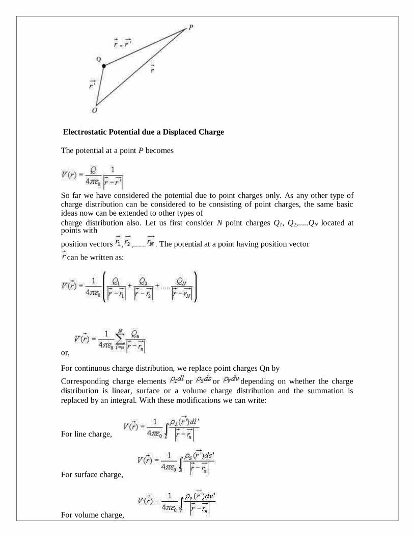
Electrostatic Potential due a Displaced Charge

The potential at a point P becomes

So far we have considered the potential due to point charges only. As any other type of charge distribution can be considered to be consisting of point charges, the same basic ideas now can be extended to other types of charge distribution also. Let us first consider N point charges Q1, Q2,.....QN located at points with

position vectors , ,...... . The potential at a point having position vector

can be written as:

or,

For continuous charge distribution, we replace point charges Qn by

Corresponding charge elements or or depending on whether the charge

distribution is linear, surface or a volume charge distribution and the summation is

replaced by an integral. With these modifications we can write:

For line charge,

For surface charge,

For volume charge,

It may be noted here that the primed coordinates represent the source coordinates and the un-primed coordinates represent field point. Further, in our discussion so far we have used the reference or zero potential at infinity. If any other point is chosen as reference, we can write:

where C is a constant. In the same manner when potential is computed from a known electric field we can write:

The potential difference is however independent of the choice of reference.

We have mentioned that electrostatic field is a conservative field; the work done in

moving a charge from one point to the other is independent of the path. Let us consider

moving a charge from point P1 to P2 in one path and then from point P2 back to P1 over a

different path. If the work done on the two paths were different, a net positive or negative

amount of work would have been done when the body returns to its original position P1.

In a conservative field there is no mechanism for dissipating energy corresponding to any

positive work neither any source is present from which energy could be absorbed in the

case of negative work. Hence the question of different works in two paths is untenable,

the work must have to be independent of path and depends on the initial and final

positions.

Since the potential difference is independent of the paths taken, VAB = - VBA , and over a

closed path,

Applying Stokes's theorem, we can write:

from which it follows that for electrostatic field,

Any vector field that satisfies is called an irrotational field.

From our definition of potential, we can write

from which we obtain,

From the foregoing discussions we observe that the electric field strength at any point

is the negative of the potential gradient at any point, negative sign shows that is

directed from higher to lower values of .

This gives us another method of computing the electric field, i. e. if we know the

potential function, the electric field may be computed. We may note here that that one

scalar function contain all the information that three components of carry, the same

is possible because of the fact that three

components of are interrelated by the relation .

Example: Electric Dipole

An electric dipole consists of two point charges of equal magnitude but of opposite sign and separated by a small distance.

As shown in figure 2.11, the dipole is formed by the two point charges Q and -Q separated by a distance d , the charges being placed symmetrically about the origin. Let us consider a point P at a distance r, where we are interested to find the field.

Electric Dipole

The potential at P due to the dipole can be written as:

When r1 and r2>>d, we can write and .

Therefore,

We can write,

The quantity is called the dipole moment of the electric dipole.

Hence the expression for the electric potential can now be written as:

It may be noted that while potential of an isolated charge varies with distance as 1/r that of an electric dipole varies as 1/r

2 with distance.

If the dipole is not centered at the origin, but the dipole center lies at , the expression

for the potential can be written as:

The electric field for the dipole centered at the origin can be computed as

is the magnitude of the dipole moment. Once again we note that the electric field

of electric dipole varies as 1/r3 where as that of a point charge varies as 1/r

2.

2.1.3 Uniform and Non-Uniform field

Electric flux density:

As stated earlier electric field intensity or simply „Electric field' gives the strength of the field at a particular point. The electric field depends on the material media in which the field is being considered. The flux density vector is defined to be independent of the material media (as we'll see that it relates to the charge that is producing it).For a linear isotropic medium under consideration; the flux density vector is defined as:

We define the electric flux as

Gauss's Law: Gauss's law is one of the fundamental laws of electromagnetism and it states that the total electric flux through a closed surface is equal to the total charge enclosed by the surface.

Gauss's Law

Let us consider a point charge Q located in an isotropic homogeneous medium of dielectric constant . The flux density at a distance r on a surface enclosing the charge is given by

If we consider an elementary area ds, the amount of flux passing through the elementary area is given by

But , is the elementary solid angle subtended by the area at the location

of Q. Therefore we can write

For a closed surface enclosing the charge, we can write

which can seen to be same as what we have stated in the definition of Gauss's Law.

Application of Gauss's Law

Gauss's law is particularly useful in computing or where the charge distribution has

some symmetry. We shall illustrate the application of Gauss's Law with some examples.

1. Infinite Sheet of Charge

As a second example of application of Gauss's theorem, we consider an infinite charged sheet covering the x-z plane as shown in figure 2.5.

Assuming a surface charge density of for the infinite surface charge, if we consider a

cylindrical volume having sides placed symmetrically as shown in figure 5, we can

write:

..............(2.17)

Infinite Sheet of Charge

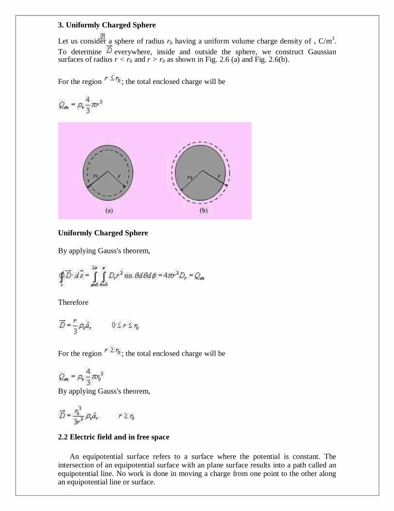
3. Uniformly Charged Sphere

Let us consider a sphere of radius r0 having a uniform volume charge density of v C/m3.

To determine everywhere, inside and outside the sphere, we construct Gaussian surfaces of radius r < r0 and r > r0 as shown in Fig. 2.6 (a) and Fig. 2.6(b).

For the region ; the total enclosed charge will be

Uniformly Charged Sphere

By applying Gauss's theorem,

Therefore

For the region ; the total enclosed charge will be

By applying Gauss's theorem,

2.2 Electric field and in free space

An equipotential surface refers to a surface where the potential is constant. The intersection of an equipotential surface with an plane surface results into a path called an equipotential line. No work is done in moving a charge from one point to the other along an equipotential line or surface.

In figure the dashes lines show the equipotential lines for a positive point charge. By symmetry, the equipotential surfaces are spherical surfaces and the equipotential lines are circles. The solid lines show the flux lines or electric lines of force. Michael Faraday as a way of visualizing electric fields introduced flux lines. It may be seen that the electric flux lines and the equipotential lines are normal to each other.

In order to plot the equipotential lines for an electric dipole, we observe

that for a given Q and d, a constant V requires that is a constant. From this we can write to be the equation for an equipotential surface and a family of surfaces

can be gener ated for various values of cv.When plotted in 2-D this would

give equipotential lines.

Fig Equipotential Lines for a Positive Point Charge

2.2.1. Electric field in conductors

As the first example of illustration of use of Gauss's law, let consider the problem of determination of the electric field produced by an infinite line charge of density LC/m. Let us consider a line charge positioned along the z-axis as shown in Fig. 2.4(a) (next slide). Since the line charge is assumed to be infinitely long, the electric field will be of the form as shown in Fig. 2.4(b) (next slide).

If we consider a close cylindrical surface as shown in Fig. 2.4(a), using Gauss's theorm we can write,

.....................................(2.15)

Considering the fact that the unit normal vector to areas S1 and S3 are perpendicular to the electric field, the surface integrals for the top and

bottom surfaces evaluates to zero. Hence we can write,

Fig : Infinite Line Charge

.....................................(2.16)

2.2.2 Electric field in dielectrics

The parameter conductivity is used characterizes the macroscopic electrical property of a

material medium. The notion of conductivity is more important in dealing with the current flow

and hence the same will be considered in detail later on.

If some free charge is introduced inside a conductor, the charges will experience a force due to

mutual repulsion and owing to the fact that they are free to move, the charges will appear on the

surface. The charges will redistribute themselves in such a manner that the field within the

conductor is zero. Therefore, under steady condition, inside a conductor

.

From Gauss's theorem it follows that

= 0

The surface charge distribution on a conductor depends on the shape of the conductor. The

charges on the surface of the conductor will not be in equilibrium if there is a tangential

component of the electric field is present, which would produce movement of the charges.

Hence under static field conditions, tangential component of the electric field on the conductor

surface is zero. The electric field on the surface of the conductor is normal everywhere to

the surface . Since the tangential component of electric field is zero, the conductor surface is

an equipotential surface.

2.3. Dielectric polarization & Dielectric strength

Here we briefly describe the behaviour of dielectrics or insulators when placed in static

electric field. Ideal dielectrics do not contain free charges. As we know, all material media are

composed of atoms where a positively charged nucleus (diameter ~ 10-15

m) is surrounded by

negatively charged electrons (electron cloud has radius ~ 10-10

m) moving around the nucleus.

Molecules of dielectrics are neutral macroscopically; an externally applied field causes small

displacement of the charge particles creating small electric dipoles. These induced dipole

moments modify electric fields both inside and outside dielectric material.

Molecules of some dielectric materials posses permanent dipole moments even in the

absence of an external applied field. Usually such molecules consist of two or more dissimilar

atoms and are called polar molecules. A common example of such molecule is water molecule

H2O. In polar molecules the atoms do not arrange themselves to make the net dipole moment

zero. However, in the absence of an external field, the molecules arrange themselves in a

random manner so that net dipole moment over a volume becomes zero. Under the influence of

an applied electric field, these dipoles tend to align themselves along the field as shown in

figure 2.15. There are some materials that can exhibit net permanent dipole moment even in the

absence of applied field. These materials are called electrets that made by heating certain waxes

or plastics in the presence of electric field. The applied field aligns the polarized molecules

when the material is in the heated state and they are frozen to their new position when after the

temperature is brought down to its normal temperatures. Permanent polarization remains

without an externally applied field.

As a measure of intensity of polarization, polarization vector (in C/m2) is

In being the number of molecules per unit volume i.e. is the dipole moment per unit volume.

Let us now consider a dielectric material having polarization and compute the potential at an

external point O due to an elementary dipole dv'.

Potential at an External Point due to an Elementary Dipole dv'.

With reference to the figure 2.16, we can write:

Therefore,

where x,y,z represent the coordinates of the external point O and x',y',z' are the coordinates of the source point.

From the expression of R, we can verify that

2.3.2 Electric field in multiple dielectrics

A dielectric medium is said to be linear when is independent of and the medium is

homogeneous if is also independent of space coordinates. A linear homogeneous and

isotropic medium is called a simple medium and for such medium the relative permittivity is a

constant.

Dielectric constant may be a function of space coordinates. For anistropic materials, the

dielectric constant is different in different directions of the electric field, D and E are related by

a permittivity tensor which may be written as:

For crystals, the reference coordinates can be chosen along the principal axes, which make off diagonal elements of the permittivity matrix zero. Therefore, we have

Media exhibiting such characteristics are called biaxial. Further, if then the medium is

called uniaxial. It may be noted that for isotropic

media, . Lossy dielectric materials are represented by a complex dielectric constant, the imaginary part of which provides the power loss in the medium and this is in general dependant on frequency.

2.4 Boundary Conditions

Let us consider the relationship among the field components that exist at the interface between two dielectrics as shown in the figure 2.17. The

permittivity of the medium 1 and medium 2 are and respectively and the interface may

also have a net charge density Coulomb/m.

Boundary Conditions at the interface between two dielectrics

We can express the electric field in terms of the tangential and normal

where Et and En are the tangential and normal components of the electric field respectively. Let us assume that the closed path is very small so that over the elemental path length the variation of E can be neglected. Moreover very near to the

interface, . Therefore

Thus, we have,

or i.e. the tangential component of an electric field is continuous across

the interface.

For relating the flux density vectors on two sides of the interface we apply Gauss‟s law to a

small pillbox volume as shown in the figure. Once again as , we can write

i.e.,

.e., Thus we find that the normal component of the flux density vector D is discontinuous across an interface by an amount of discontinuity equal to the surface charge density at the interface.

2.5 Poisson’s and Laplace’s Equations

For electrostatic field, we have seen that

Form the above two equations we can write

Using vector identity we can write,

For a simple homogeneous medium, is constant and . Therefore,

This equation is known as Poisson’s equation. Here we have introduced a new operator, ( del square), called the Laplacian operator. In Cartesian coordinates,

Therefore, in Cartesian coordinates, Poisson equation can be written as:

In cylindrical coordinates,

In spherical polar coordinate system,

At points in simple media, where no free charge is present, Poisson‟s equation reduces to

which is known as Laplace‟s equation.

Laplace‟s and Poisson‟s equation are very useful for solving many practical electrostatic field problems where only the electrostatic conditions (potential and charge) at some boundaries are known and solution of electric field and potential is to be found throughout the volume. We shall consider such applications in the section where we deal with boundary value problems.

2.6 Capacitance and Capacitors

We have already stated that a conductor in an electrostatic field is an Equipotential body and any charge given to such conductor will distribute themselves in such a manner that electric field inside the conductor vanishes. If an additional amount of charge is supplied to an isolated conductor at a given potential, this additional charge will increase the

surface charge density . Since the potential of the conductor is given by

, the potential of the conductor will also increase

maintaining the ratio same. Thus we can write where the constant of proportionality

C is called the capacitance of the isolated conductor. SI unit of capacitance is Coulomb/ Volt

also called Farad denoted by F. It can It can be seen that if V=1, C = Q.

Thus capacity of an isolated conductor can also be defined as the amount of charge in

Coulomb required to raise the potential of the conductor by 1 Volt. Of considerable interest in

practice is a capacitor that consists of two (or more) conductors carrying equal and opposite

charges and separated by some dielectric media or free space. The conductors may have

arbitrary shapes. A two-conductor capacitor is shown in figure

Capacitance and Capacitors

When a d-c voltage source is connected between the conductors, a charge transfer occurs which results into a positive charge on one conductor and negative charge on the other conductor. The conductors are equipotential surfaces and the field lines are perpendicular to the conductor surface. If V is the mean potential difference between the conductors, the capacitance is given

by . Capacitance of a capacitor depends on the geometry of the conductor and the permittivity of the medium between them and does not depend on the charge or potential difference between conductors. The capacitance can be computed by assuming Q(at the same

time -Q on the other conductor), first determining using Gauss‟s theorem and then

determining . We illustrate this procedure by taking the example of a parallel plate

capacitor.

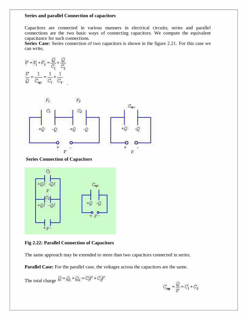
Series and parallel Connection of capacitors

Capacitors are connected in various manners in electrical circuits; series and parallel connections are the two basic ways of connecting capacitors. We compute the equivalent capacitance for such connections. Series Case: Series connection of two capacitors is shown in the figure 2.21. For this case we can write,

.

Series Connection of Capacitors

Fig 2.22: Parallel Connection of Capacitors

The same approach may be extended to more than two capacitors connected in series.

Parallel Case: For the parallel case, the voltages across the capacitors are the same.

The total charge

2.6.1 Energy Density

We have stated that the electric potential at a point in an electric field is the amount of work

required to bring a unit positive charge from infinity (reference of zero potential) to that point.

To determine the energy that is present in an assembly of charges, let us first determine the

amount of work required to assemble them. Let us consider a number of discrete charges Q1,

Q2,......., QN are brought from infinity to their present position one by one. Since initially there

is no field present, the amount of work done in bring Q1 is zero. Q2 is brought in the presence

of the field of Q1, the work done W1= Q2V21 where V21 is the potential at the location of Q2 due

to Q1. Proceeding in this manner, we can write, the total work done

Had the charges been brought in the reverse order,

Therefore,

Here VIJ represent voltage at the Ith

charge location due to Jth charge. Therefore,

Or,

If instead of discrete charges, we now have a distribution of charges over a volume v then we can write,

where is the volume charge density and V represents the potential function.

Since, , we can write

Using the vector identity,

, we can write

................(2.95)

In the expression , for point charges, since V varies as and D varies as , the

term V varies as while the area varies as r2. Hence the integral term varies at least as and

the as surface becomes large (i.e.

) the integral term tends to zero.

Thus the equation for W reduces to

, is called the energy density in the electrostatic field.

Unit III Magneto statics

3.1. Introduction to Magneto statics In previous chapters we have seen that an electrostatic field is produced by static or stationary charges.

The relationship of the steady magnetic field to its sources is much more complicated.

The source of steady magnetic field may be a permanent magnet, a direct current or an electric field changing with time. In this chapter we shall mainly consider the magnetic field produced by a direct current. The magnetic field produced due to time varying electric field will be discussed later. Historically, the link between the electric and magnetic field was established Oersted in 1820. Ampere and others extended the investigation of magnetic effect of electricity. 3.2. Lorentz force

Lorentz force is the combination of electric and magnetic force on a point charge due to electromagnetic fields. A particle

of charge q moving with velocity v in the presence of an electric field E and a magnetic field B experiences a force

There are two major laws governing the magnetostatic fields are:

Biot-Savart Law Ampere's Law

3.2.1. Magnetic field intensity(H)

Usually, the magnetic field intensity is represented by the vector . It is customary to represent the

direction of the magnetic field intensity (or current) by a small circle with a dot or cross sign depending on

whether the field (or current) is out of or into the page as shown in Fig. 4.1.

(or l ) out of the page (or l ) into the page

Representation of magnetic field (or current)

3.3. Biot–Savart’s Law

This law relates the magnetic field intensity dH produced at a point due to a differential current element

as shown in Fig. 4.2.

Magnetic field intensity due to a current element

The magnetic field intensity at P can be written as,

where is the distance of the current element from the point P.

Similar to different charge distributions, we can have different current distribution such as line current, surface current and volume current. These different types of current densities are shown in Fig. 4.3.

Line Current Surface Current Volume Current

Different types of current distributions

By denoting the surface current density as K (in amp/m) and volume current density as J (in amp/m

2) we can

write:

.

( It may be noted that )

Employing Biot-Savart Law, we can now express the magnetic field intensity H. In terms of

These current distributions.

............................. for line current

........................ for surface current

....................... for volume current......................

3.3.1 Ampere's Circuital Law:

Ampere's circuital law states that the line integral of the magnetic field (circulation of H ) around a

closed path is the net current enclosed by this path. Mathematically,

The total current I enc can be written as,

By applying Stoke's theorem, we can write

which is the Ampere's law in the point form. 3.4. H due to straight conductors

In simple matter, the magnetic flux density related to the magnetic field intensity as where called

the permeability. In particular when we consider the free space

where H/m is the permeability of the free space. Magnetic flux density is measured in terms of

Wb/m 2 .

The magnetic flux density through a surface is given by:

Wb In the case of electrostatic field, we have seen that if the surface is a closed surface, the net flux passing through the surface is equal to the charge enclosed by the surface. In case of magnetic field isolated magnetic charge (i. e. pole) does not exist. Magnetic poles always occur in pair (as N-S). For example, if we desire to have an isolated magnetic pole by dividing the magnetic bar successively into two, we end up with pieces each having north (N) and south (S) pole as shown in Fig. 4.7 (a). This process could be continued until the magnets are of atomic dimensions; still we will have N-S pair occurring together. This means that the magnetic poles cannot be isolated.

(a) Subdivision of a magnet (b) Magnetic field/ flux lines of a straight current carrying conductor

Similarly if we consider the field/flux lines of a current carrying conductor as shown in Fig. 4.7 (b), we find that these lines are closed lines, that is, if we consider a closed surface, the number of flux lines that would leave the surface would be same as the number of flux lines that would enter the surface.

From our discussions above, it is evident that for magnetic field,

which is the Gauss's law for the magnetic field.

By applying divergence theorem, we can write:

Hence,

which is the Gauss's law for the magnetic field in point form.

3.4.1 H due to circular loop

A current carrying wire generates a magnetic field. According to Biot-Savart‟s law, the magnetic field at a

point due to an element of a conductor carrying current is,

Directly proportional to the strength of the current, i

1. Directly proportional to the length of the element, dl

2. Directly proportional to the Sine of the angle θ between the element and the line joining the element to the

point and

3. Inversely proportional to the square of the distance r between the element and the point.

Thus, the magnetic field at O is dB, such that,

Then,

where,

.

In vector form,

Consider a circular coil of radius r, carrying a current I. Consider a point P, which is at a distance x from the centre of the coil.

We can consider that the loop is made up of a large number of short elements, generating small magnetic fields. So the total field

at P will be the sum of the contributions from all these elements. At the centre of the coil, the field will be uniform. As the

location of the point increases from the centre of the coil, the field decreases.

By Biot- Savart‟s law, the field dB due to a small element dl of the circle, centered at A is given by,

This can be resolved into two components, one along the axis OP, and other PS, which is perpendicular to OP.

PS is exactly cancelled by the perpendicular component PS‟ of the field due to a current and centered at A‟. So, the

total magnetic field at a point which is at a distance x away from the axis of a circular coil of radius r is given by,

If there are n turns in the coil, then

where µ0 is the absolute permeability of free space. Since this field Bx from the coil is acting perpendicular to the

horizontal intensity of earth‟s magnetic field, B0, and the compass needle align at an angle θ with the vector sum of

these two fields, we have from the figure

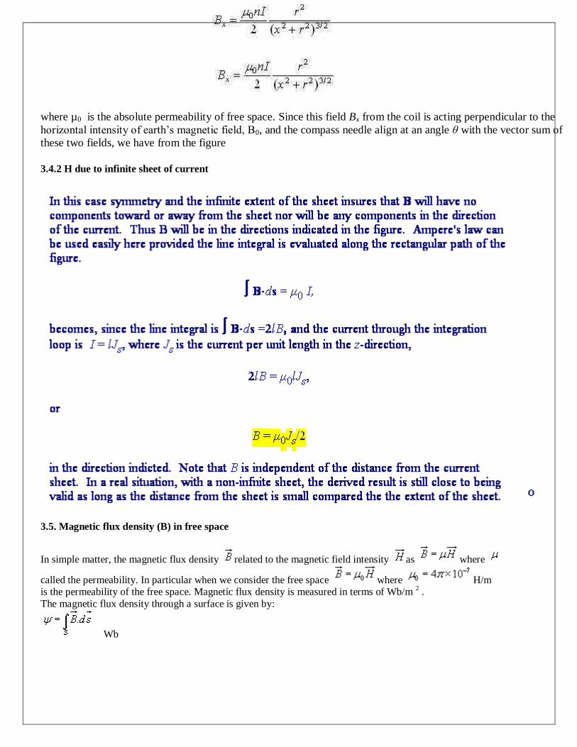
3.4.2 H due to infinite sheet of current

3.5. Magnetic flux density (B) in free space

In simple matter, the magnetic flux density related to the magnetic field intensity as where

called the permeability. In particular when we consider the free space where H/m is the permeability of the free space. Magnetic flux density is measured in terms of Wb/m

2 .

The magnetic flux density through a surface is given by:

Wb

3.5.1 Magnetic flux density (B) in conductor

Students will probably know that electric and gravitational fields are defined as the force on unit charge

or mass. So by comparison, B = F/IL, and this gives a way of defining the 'magnetic field strength'.

Physicists refer to this as the B-field or magnetic flux density which has units of N A-1

m-1 or tesla (T).

A field of 1T is a very strong field. The field between the poles of the Magnadur magnets that are used

in the above experiment is about 3 ́10-2

T while the Earth's magnetic field is about 10-5 T.

If your specification requires, you will need to develop the 'angle factor' seen in the experiment into the

mathematical formula:

F = BIL sin q .

For the mathematically inclined, it can be shown that the effective length of the wire in the field (i.e. that which is at right

angles) is L sin q. If students find this difficult, then it can be argued that the maximum force occurs when field and current

are at right angles, q = 90o (sin q = 1), and that this falls to zero when field and current are parallel, q = 0

o (sin q = 0).

Discussion: Formal definitions

Some specifications require a formal definition of magnetic flux density and/or the tesla. The strength of a magnetic field or

magnetic flux density B can be measured by the force per unit current per unit length acting on a current-carrying conductor

placed perpendicular to the lines of a uniform magnetic field. The SI unit of magnetic flux density B is the tesla (T), equal to

1 N A–1

m–1

. This is the magnetic flux density if a wire of length 1m carrying a current of 1 A as a force of 1 N exerted on it

in a direction perpendicular to both the flux and the current. Study of the force between parallel conductors leading to the

definition of the ampere may be required. Students may already have seen the effect in your initial experiments but this may

need to be repeated here. The effect can be explained by considering the effect of the field produced by one conductor on the

other and then reversing the argument.

The force between parallel conductors forms the basis of the definition of the unit of current, the ampere. A formal

definition is not usually required but students should realize that in a current balance (such as was used above)

measurement of force and length can be traced back to fundamental SI units (kg, m, s) leaving the current as the only

'unknown‟. Some students are likely to be interested in the formal definition which is "that constant current which, if

maintained in two straight parallel conductors of infinite length, of negligible cross-section, and placed 1m apart in a

vacuum, would produce a force of 2 ´ 10-7

Newton per metre of length".

3.6 Magnetic materials

The origin of magnetism lies in the orbital and spin motions of electrons and how the electrons interact with one another. The

best way to introduce the different types of magnetism is to describe how materials respond to magnetic fields. This may be

surprising to some, but all matter is magnetic. It's just that some materials are much more magnetic than others. The main

distinction is that in some materials there is no collective interaction of atomic magnetic moments, whereas in other materials

there is a very strong interaction between atomic moments

3.6.1 Types and properties

1. Diamagnetism

Diamagnetism is a fundamental property of all matter, although it is usually very weak. It is due to the non-cooperative

behavior of orbiting electrons when exposed to an applied magnetic field. Diamagnetic substances are composed of atoms

which have no net magnetic moments (ie., all the orbital shells are filled and there are no unpaired electrons). However,

when exposed to a field, a negative magnetization is produced and thus the susceptibility is negative. If we plot M vs H,

2. Paramagnetism

This class of materials, some of the atoms or ions in the material have a net magnetic moment due to unpaired electrons in

partially filled orbitals. One of the most important atoms with unpaired electrons is iron. However, the individual magnetic

moments do not interact magnetically, and like diamagnetism, the magnetization is zero when the field is removed. In the

presence of a field, there is now a partial alignment of the atomic magnetic moments in the direction of the field, resulting

in a net positive magnetization and positive susceptibility.

3. Ferromagnetism

When you think of magnetic materials, you probably think of iron, nickel or magnetite. Unlike paramagnetic

materials, the atomic moments in these materials exhibit very strong interactions. These interactions are produced by

electronic exchange forces and result in a parallel or antiparallel alignment of atomic moments. Exchange forces are

very large, equivalent to a field on the order of 1000 Tesla, or approximately a 100 million times the strength of the

earth's field. The exchange force is a quantum mechanical phenomenon due to the relative orientation of the spins of

two electron. Ferromagnetic materials exhibit parallel alignment of moments resulting in large net magnetization even

in the absence of a magnetic field.

4. Ferrimagnetism

In ionic compounds, such as oxides, more complex forms of magnetic ordering can occur as a result of the crystal

structure. One type of magnetic ordering is call ferrimagnetism.

3.7.Magnetization

magnetic polarization is the vector field that expresses the density of permanent or induced magnetic dipole moments

in a magnetic material. The origin of the magnetic moments responsible for magnetization can be either microscopic

electric currents resulting from the motion of electrons in atoms, or the spin of the electrons or the nuclei.

Net magnetization results from the response of a material to an external magnetic field, together with any unbalanced

magnetic dipole moments that may be inherent in the material itself.

3.7.1 Magnetic field in multiple media

Similar to the boundary conditions in the electro static fields, here we will consider the behavior of and at

the interface of two different media. In particular, we determine how the tangential and normal components of

magnetic fields behave at the boundary of two regions having different permeabilities.

The figure 4.9 shows the interface between two media

permeabities and , being the normal having

vector from medium 2 to medium 1.

Interface between two magnetic media

To determine the condition for the normal component of the flux density vector , we consider a small pill box

P with vanishingly small thickness h and having an elementary area for the faces. Over the pill box, we can

write

Since h --> 0, we can neglect the flux through the sidewall of the pill box. where

Since is small, we can write

or,

That is, the normal component of the magnetic flux density vector is continuous across the interface.

In vector form,

and.................. (4.38)

To determine the condition for the tangential component for the magnetic field, we consider a closed path C as shown in figure 4.8. By applying Ampere's law we can write

Since h -->0,

We have shown in figure 4.8, a set of three unit vectors , and such that they satisfy

(R.H. rule). Here is tangential to the interface and is the vector perpendicular to the surface

enclosed by C at the interface 3.9 Scalar and Vector Potentials:

In studying electric field problems, we introduced the concept of electric potential that simplified the computation Divergence theorem n of electric fields for certain types of problems. In the same manner let us relate the magnetic field intensity to a scalar magnetic potential and write:

From Ampere's law , we know that

But using vector identity, we find that is valid only where . Thus the

scalar magnetic potential is defined only in the region where . Moreover, Vm in general is not a single valued function of position.This point can be illustrated as follows. Let us consider the cross section of a coaxial line as shown in fig

In the region , and

Cross Section of a Coaxial Line

If Vm is the magnetic potential then,

If we set Vm = 0 at then c=0 and

We observe that as we make a complete lap around the current carrying conductor , we reach again but Vm this time becomes

We observe that value of Vm keeps changing as we complete additional laps to pass through the same point. We introduced Vm analogous to electostatic potential V. But for static electric

fields, and , whereas for steady magnetic field wherever but

even if along the path of integration.

We now introduce the vector magnetic potential which can be used in regions where current density may be zero or nonzero and the same can be easily extended to time varying cases. The use of vector magnetic potential provides elegant ways of solving EM field problems.

Since and we have the vector identity that for any vector , , we can write

.

Here, the vector field is called the vector magnetic potential. Its SI unit is Wb/m. Thus if can find of a given

current distribution, can be found from through a curl operation.

Unit IV Electrodynamic fields

4.1.Introduction to electro dynamic fields

In our study of static fields so far, we have observed that static electric fields are produced by electric charges, static magnetic fields are produced by charges in motion or by steady current. Further, static electric field is a conservative field and has no curl, the static magnetic field is continuous and its divergence is zero.

4.2. Concept of Magnetic Circuits

The fundamental relationships for static electric fields among the field quantities can

be summarized as:

(5.1a)

(5.1b)

For a linear and isotropic medium,

(5.1c)

Similarly for the magnetostatic case

(5.2a)

(5.2b)

(5.2c)

It can be seen that for static case, the electric field vectors and and magnetic field

vectors and form separate pairs.

In this chapter we will consider the time varying scenario. In the time varying case we will observe that a changing magnetic field will produce a changing electric field and vice versa.

4.3. Study on Faraday’s law

Michael Faraday, in 1831 discovered experimentally that a current was induced in a conducting loop when the magnetic flux linking the loop changed. In terms of fields, we

can say that a time varying magnetic field produces an electromotive force (emf) which causes a current in a closed circuit. The quantitative relation between the induced emf (the voltage that arises from conductors moving in a magnetic field or from changing magnetic fields) and the rate of change of flux linkage developed based on experimental

observation is known as Faraday's law. Mathematically, the induced emf can be written as

Emf = Volts (5.3)

where is the flux linkage over the closed path.

A non zero may result due to any of the following:

(a) time changing flux linkage a stationary closed path.

(b) relative motion between a steady flux a closed path.

(c) a combination of the above two cases.

4.4. Transformer and motional EMF

The negative sign in equation (5.3) was introduced by Lenz in order to comply with the polarity of the induced emf. The negative sign implies that the induced emf will cause a current flow in the closed loop in such a direction so as to oppose the change in the linking magnetic flux which produces it. (It may be noted that as far as the induced emf is concerned, the closed path forming a loop does not necessarily have to be conductive).

If the closed path is in the form of N tightly wound turns of a coil, the change in the magnetic flux linking the coil induces an emf in each turn of the coil and total emf is the sum of the induced emfs of the individual turns, i.e.,

Emf =

Volts (5.4)

By defining the total flux linkage as

(5.5)

The emf can be written as

Emf = (5.6)

Continuing with equation (5.3), over a closed contour 'C' we can write

Emf = (5.7)

where is the induced electric field on the conductor to sustain the

current.

Further, total flux enclosed by the contour 'C ' is given by

(5.8)

Where S is the surface for which 'C' is the contour.

From (5.7) and using (5.8) in (5.3) we can write

(5.9)

By applying stokes theorem

(5.10)

Therefore, we can write

(5.11)

which is the Faraday's law in the point form

We have said that non zero can be produced in a several ways. One particular case is

when a time varying flux linking a stationary closed path induces an emf. The emf

induced in a stationary closed path by a time varying magnetic field is called a

transformer emf .

Example: Ideal transformer

As shown in figure 5.1, a transformer consists of two or more numbers of coils coupled magnetically through a common core. Let us consider an ideal transformer whose winding has zero resistance, the core having infinite permittivity and magnetic losses are zero.

Transformer with secondary open

These assumptions ensure that the magnetization current under no load condition is

vanishingly small and can be ignored. Further, all time varying flux produced by the

primary winding will follow the magnetic path inside the core and link to the secondary

coil without any leakage. If N1 and N2 are the number of turns in the primary and the

secondary windings respectively, the induced emfs are

(5.12a)

(5.12b)

(The polarities are marked, hence negative sign is omitted. The induced emf is +ve at the dotted end of the winding.)

(5.13)

i.e., the ratio of the induced emfs in primary and secondary is equal to the ratio of their

turns. Under ideal condition, the induced emf in either winding is equal to their voltage

rating.

(5.14)

where 'a' is the transformation ratio. When the secondary winding is connected to a load,

the current flows in the secondary, which produces a flux opposing the original flux. The

net flux in the core decreases and induced emf will tend to decrease from the no load

value. This causes the primary current to increase to nullify the decrease in the flux and

induced emf. The current continues to increase till the flux in the core and the induced

emfs are restored to the no load values. Thus the source supplies power to the primary

winding and the secondary winding delivers the power to the load. Equating the powers

(5.15)

(5.16)

Further,

(5.17)

i.e., the net magnetomotive force (mmf) needed to excite the transformer is zero under ideal condition.

Motional EMF:

Let us consider a conductor moving in a steady magnetic field as shown in the fig 5.2.

Fig 5.2

If a charge Q moves in a magnetic field , it experiences a force

(5.18)

This force will cause the electrons in the conductor to drift towards one end and leave the other end positively charged, thus creating a field and charge separation continuous until electric and magnetic forces balance and an equilibrium is reached very quickly, the net force on the moving conductor is zero.

can be interpreted as an induced electric field which is called the motional

electric field

(5.19)

If the moving conductor is a part of the closed circuit C, the generated emf

around the circuit is . This emf is called the motional emf.

A classic example of motional emf is given in Additonal Solved Example No.1 .

4.6.Maxwell’s equations

Equation (5.1) and (5.2) gives the relationship among the field quantities in the static field. For time varying case, the relationship among the field vectors written as

(5.20a)

(5.20b)

(5.20c)

(5.20d)

In addition, from the principle of conservation of charges we get the equation of continuity

(5.21) The equation 5.20 (a) - (d) must be consistent with equation (5.21).

We observe that

(5.22)

Since is zero for any vector .

Thus applies only for the static case i.e., for the scenario when

. A classic example for this is given below .

Suppose we are in the process of charging up a capacitor as shown in fig 5.3.

Fig 5.3

Let us apply the Ampere's Law for the Amperian loop shown in fig 5.3. Ienc = I is the total current passing through the loop. But if we draw a baloon shaped surface as in fig 5.3, no current passes through this surface and hence Ienc = 0. But for non steady currents such as this one, the concept of current enclosed by a loop is ill-defined since it depends on what surface you use. In fact Ampere's Law should also hold true for time varying case as well, then comes the idea of displacement current which will be introduced in the next few slides.

We can write for time varying case,

(5.23)

(5.24)

The equation (5.24) is valid for static as well as for time varying case.

Equation (5.24) indicates that a time varying electric field will give rise to a

magnetic field even in the absence of . The term has a dimension of

current densities and is called the displacement current density.

Introduction of in equation is one of the major contributions of Jame's Clerk

Maxwell. The modified set of equations

(5.25a)

(5.25b)

(5.25c)

(5.25d)

is known as the Maxwell's equation and this set of equations apply in the

time varying scenario, static fields are being a particular case .

In the integral form

(5.26a)

(5.26b)

(5.26c)

(5.26d)

The modification of Ampere's law by Maxwell has led to the development of a unified electromagnetic field theory. By introducing the displacement current term, Maxwell could predict the propagation of EM waves. Existence of EM waves was later demonstrated by Hertz experimentally which led to the new era of radio communication.

Boundary Conditions for Electromagnetic fields

The differential forms of Maxwell's equations are used to solve for the field vectors provided the field quantities are single valued, bounded and continuous. At the media

boundaries, the field vectors are discontinuous and their behaviors across the boundaries are governed by boundary conditions. The integral equations(eqn 5.26) are assumed to

hold for regions containing discontinuous media.Boundary conditions can be derived by applying the Maxwell's equations in the integral form to small regions at the interface of

the two media. The procedure is similar to those used for obtaining boundary conditions for static electric fields (chapter 2) and static magnetic fields (chapter 4). The boundary

conditions are summarized as follows

Equation 5.27 (a) says that tangential component of electric field is continuous across the

interface while from 5.27 (c) we note that tangential component of the magnetic field is

discontinuous by an amount equal to the surface current density. Similarly 5.27 (b) states

that normal component of electric flux density vector is discontinuous across the

interface by an amount equal to the surface current density while normal component of

the magnetic flux density is continuous. If one side of the interface, as shown in fig 5.4, is

a perfect electric

Wave equation and their solution:

From equation 5.25 we can write the Maxwell's equations in the differential form as

Let us consider a source free uniform medium having dielectric constant , magnetic

permeability and conductivity . The above set of equations can be written as

Using the vector identity ,

We can write from 5.29(b)

or

Substituting from 5.29(a)

But in source free medium (eqn 5.29(c))

(5.30)

In the same manner for equation eqn 5.29(a)

Since from eqn 5.29(d), we can write

(5.31)

These two equations

are known as wave equations.

It may be noted that the field components are functions of both space and time. For

example, if we consider a Cartesian co ordinate system,

essentially represents and . For simplicity, we consider

propagation in free space , i.e. , and . The wave eqn in equations 5.30

and 5.31 reduces to

Further simplifications can be made if we consider in Cartesian co ordinate

system a special case where are considered to be independent in

two dimensions, say are assumed to be independent of y and z. Such waves are called plane waves.

From eqn (5.32 (a)) we can write

The vector wave equation is equivalent to the three scalar equations

Since we have ,

As we have assumed that the field components are independent of y and z eqn (5.34) reduces to

(5.35)

i.e. there is no variation of Exin the x direction.

Further, from 5.33(a), we find that implies which requires any three of

the conditions to be satisfied: (i) Ex=0, (ii)Ex = constant, (iii)Ex increasing uniformly with

time. A field component satisfying either of the last two conditions (i.e (ii) and (iii))is not a part of a plane wave motion and hence Ex is taken to be equal to zero. Therefore, a uniform plane wave propagating in x direction does not have a field component (E or H) acting along x.

Without loss of generality let us now consider a plane wave having Ey component only (Identical results can be obtained for Ez component) .

The equation involving such wave propagation is given by

The above equation has a solution of the form

where

Thus equation (5.37) satisfies wave eqn (5.36) can be verified by substitution.

corresponds to the wave traveling in the + x direction while

corresponds to a wave traveling in the -x direction. The general solution of the

wave eqn thus consists of two waves, one traveling away from the source and other

traveling back towards the source. In the absence of any reflection, the second form of

the eqn (5.37) is zero and the solution can be written as

(5.38) Such a wave motion is graphically shown in fig 5.5 at two instances of time t1 and t2.

Traveling wave in the + x direction

Let us now consider the relationship between E and H components for the

Forward travelling wave.

Since and there is no variation along y and z.

Since only z component of exists, from (5.29(b))

(5.39)

and from (5.29(a)) with , only Hz component of magnetic field being present

(5.40)

Substituting Ey from (5.38)

The constant of integration means that a field independent of x may also exist. However, this field will not be a part of the wave motion.

Hence (5.41)

which relates the E and H components of the traveling wave.

is called the characteristic or intrinsic impedance of the free space

4.7. Relation between field theory and circuit theory

Circuit Theory:

1) This analysis is originated by its own.

2) Applicable only for portion of radiofrequency range.

3) It is dependent and independent parameter, I and V are directly obtained from the given circuit.

4) Parameters of medium are not involved.

5) Laplace Transform is employed.

6) Z, Y and H parameters are used.

7) Low power is involved.

8) Simple to understand.

9) 2 Dimensional analysis.

10) Frequency is used for reference.

11) Lumped components are used.

Field Theory:

1) Evolved from transmission ratio.

2) Not applicable for portion of radiofrequency range.

3) Not directly obtained from E and H.

4) Parameters (Permeability and Permitiviy) are analysed in the medium.

5) Maxwell's equation is used.

6) S parameter is used.

7) High Power is involved.

8) Needs visualisation effect.

9) 3 Dimensional analysis.

10) Wavelength is used as reference.

11) Distributed components are used.

4.7.1 Applications

The uses and applications of Maxwell's equations are just too many to count. By understanding

electromagnetism we're able to create images of the body using MRI scanners in hospitals; we've created magnetic

tape, generated electricity, and built computers. Any device that uses electricity or magnets is on a fundamental level

built upon the original discovery of Maxwell's equations.

While using Maxwell's equations often involves calculus, there are simplified versions of the equations we can

study. These versions only work in certain circumstances, but can be useful and save a lot of trouble. Let's look

at one of these - the simplified version of Faraday's law.

As a reminder, Faraday's law says that any change to the magnetic environment of a coil of wire will cause a

voltage to be induced in the coil. And we can quantify those changes in a simple equation. Doing so gives you

this equation below, where N is the number of turns on the coil of wire, delta BA is the change in the magnetic

field times the area of the coil of wire, and delta t is the time over which that change occurs.

Unit V Electromagnetic waves

5.1. Introduction to Electromagnetic waves

. The light that comes from the sun or the light from a light bulb that allows us to read in an otherwise

dark room is electromagnetic radiation. However, the electromagnetic vibrations that is possible

extend well beyond what our eyes can perceive. Similarly, radio waves that we pick up on a radio

as are the TV signals that are transmitted by our television station are also a form of this

electromagnetic radiation.

5.2.Electromagnetic wave generation and equations

The Helmhotz Equation:

In source free linear isotropic medium, Maxwell equations in phasor form are,

or,

or,

or, where

An identical equation can be derived for .

i.e.,

These equations

are called homogeneous vector Helmholtz's equation.

is called the wave number or propagation constant of the medium.

5.3. Wave parameters

Plane waves in Lossless medium:

In a lossless medium, are real numbers, so k is real.

In Cartesian coordinates each of the equations 6.1(a) and 6.1(b) are equivalent to three scalar Helmholtz's equations, one each in the components Ex, Ey and Ez or Hx , Hy, Hz.

For example if we consider Ex component we can write

.................................................(6.2)

A uniform plane wave is a particular solution of Maxwell's equation assuming electric field (and magnetic field) has same magnitude and phase in infinite planes perpendicular to the direction of propagation. It may be noted that in the strict sense a uniform plane

wave doesn't exist in practice as creation of such waves are possible with sources of infinite extent. However, at large distances from the source, the wavefront or the surface of the constant phase becomes almost spherical and a small portion of this large sphere

can be considered to plane. The characteristics of plane waves are simple and useful for studying many practical scenarios.

Let us consider a plane wave which has only Ex component and propagating along z . Since the plane wave will have no variation along the plane

perpendicular to z i.e., xy plane, . The Helmholtz's equation (6.2) reduces

to,

.........................................................................(6.3)

The solution to this equation can be written as

............................................................(6.4)

are the amplitude constants (can be determined from boundary conditions).

In the time domain,

.............................(6.5)

assuming are real constants.

Here, represents the forward traveling wave. The

plot of for several values of t is shown in the Figure 6.1.

Figure 6.1: Plane wave traveling in the + z direction

As can be seen from the figure, at successive times, the wave travels in the +z direction.

If we fix our attention on a particular point or phase on the wave (as shown

by the dot) i.e. , = constant

Then we see that as t is increased to , z also should increase to so that

Or,

Or,

When ,

we write = phase velocity .

.....................................(6.6)

If the medium in which the wave is propagating is free space i.e.,

Then

Where 'C' is the speed of light. That is plane EM wave travels in free space with the

speed of light.

5.4.Intrinsic impedance

The wavelength is defined as the distance between two successive maxima (or minima

or any other reference points).

i.e.,

or,

or,

Substituting ,

or, ................................(6.7)

Thus wavelength also represents the distance covered in one oscillation

of the wave. Similarly, represents a plane wave traveling in

the -z direction.

The associated magnetic field can be found as follows:

From (6.4),

=

=............ (6.8)

where is the intrinsic impedance of the medium.

When the wave travels in free space

is the intrinsic impedance of the free space.

In the time domain,

........... (6.9)

Which represents the magnetic field of the wave traveling in the +z direction.

For the negative traveling wave,

...........(6.10)

For the plane waves described, both the E & H fields are perpendicular to the direction of propagation, and these waves are called TEM (transverse electromagnetic) waves.

The E & H field components of a TEM wave is shown in Fig 6.2.

E & H fields of a particular plane wave at time t.

So far we have considered a plane electromagnetic wave propagating in the z-direction. Let us now consider the propagation of a uniform plane wave in any arbitrary direction that doesn't necessarily coincides with an axis.

For a uniform plane wave propagating in z-direction

is a constant vector........................... (6.11)

The more general form of the above equation is

........................................... (6.12)

This equation satisfies Helmholtz's equation provided,

........................... (6.13)

We define wave number vector ........................... (6.14)

And radius vector from the origin

........................... (6.15)

Therefore we can write

........................... (6.16)

Here =constant is a plane of constant phase and uniform amplitude just

in the case of ,

z =constant denotes a plane of constant phase and uniform amplitude.

If the region under consideration is charge free,

Using the vector identity and noting that is constant we can

write,

......................(6.17)

i.e., is transverse to the direction of the propagation.

The corresponding magnetic field can be computed as follows:

Using the vector identity,

Since is constant we can write,

.....................(6.18)

Where is the intrinsic impedance of the medium. We observe that is

perpendicular to both and . Thus the electromagnetic wave

represented by and is a TEM wave.

5.4.1propagation constant In a lossy medium, the EM wave looses power as it propagates. Such a medium is conducting with conductivity and we can write:

.....................(6.19)

Where is called the complex permittivity.

We have already discussed how an external electric field can polarize a dielectric and give rise to bound charges. When the external electric field is time varying, the polarization vector will vary with the same frequency as that of the applied field. As the frequency of the applied filed increases, the inertia of the charge particles tend to prevent the particle displacement keeping pace with the applied field changes. This results in frictional damping mechanism causing power loss.

In addition, if the material has an appreciable amount of free charges, there will be ohmic losses. It is customary to include the effect of damping and

ohmic losses in the imaginary part of . An equivalent conductivity represents

all losses.

The ratio is called loss tangent as this quantity is a measure of the power loss.

Fig 6.3 : Calculation of Loss Tangent

With reference to the Fig 6.3,

.......................... (6.20)

where is the conduction current density and is displacement current density. The

loss tangent gives a measure of how much lossy is the medium

under consideration. For a good dielectric medium is very

small and the medium is a good conductor if . A material may be a good

conductor at low frequencies but behave as lossy dielectric at higher frequencies.

For a source free lossy medium we can write

........................... (6.21)

.................... (6.22)

Where

Proceeding in the same manner we can write,

is called the propagation constant.

The real and imaginary parts and of the propagation constant can be computed as

follows:

And

................... (6.23a)

Similarly................... (6.23b)

Let us now consider a plane wave that has only x -component of electric field and propagate along z .

................................... (6.24)

Considering only the forward traveling wave

................................... (6.25)

Similarly, from , we can find

..................................... (6.26)

Where

..................................... (6.27)

From (6.25) and (6.26) we find that as the wave propagates along z, it

decreases in amplitude by a factor . Therefore is known as attenuation constant.

Further and are out of phase by an angle .

For low loss dielectric, , i.e., .

Using the above condition approximate expression for and can be obtained as

follows:

............. (6.29)

& phase velocity

............... (6.30)

For good conductors

=............... (6.31)

We have used the relation

From (6.31) we can write

............... (6.32)

..................... (6.33)

And phase velocity

..................... (6.34)

5.5.Waves in free space

Electromagnetic waves can transport energy from one point to another point. The electric and magnetic field intensities asscociated with a travelling electromagnetic wave can be related to the rate of such energy transfer.

Let us consider Maxwell's Curl Equations:

Using vector identity

the above curl equations we can write

.............................................(6.35)

In simple medium where and are constant, we can write

and

Applying Divergence theorem we can write,

...........................(6.36)

The term represents the rate of change of energy

stored in the electric and magnetic fields and the term represents the power

dissipation within the volume. Hence right hand side of the equation (6.36) represents the

total decrease in power within the volume under consideration.

The left hand side of equation (6.36) can be written as

where (W/mt2) is called the Poynting vector and it represents the power

density vector associated with the electromagnetic field. The integration of the Poynting vector over any closed surface gives the net power flowing out of the surface. Equation (6.36) is referred to as Poynting theorem and it states that the net power flowing out of a given volume is

equal to the time rate of decrease in the energy stored within the volume minus the conduction losses.

5.5.1 definition

For time harmonic case, the time variation is of the form , and we have seen that

instantaneous value of a quantity is the real part of the product

of a phasor quantity and when is used as reference. For example, if we

consider the phasor

then we can write the instanteneous field as

.................................(6.37)

when E0 is real. Let us consider two instanteneous quantities A and B such that

where A and B are the phasor quantities.

i.e,

Therefore,

..............................(6.39)

Since A and B are periodic with period , the time average value of the product

form AB, denoted by can be written as

.....................................(6.40)

Further, considering the phasor quantities A and B, we find that

and , where * denotes complex conjugate.

..............................................(6.41)

The poynting vector can be expressed as

...................................(6.42)

If we consider a plane electromagnetic wave propagating in +z direction and has only

component, from (6.42) we can write:

Using (6.41)

........................................(6.43)

where and , for the plane wave under consideration.

For a general case, we can write

.....................(6.44)

We can define a complex Poynting vector

and time average of the instantaneous Poynting vector is given by .

5.5.2 Waves in loss dielectrics

The polarisation of a plane wave can be defined as the orientation of the electric field vector as a function of time at a fixed point in space. For an electromagnetic wave, the specification of the orientation of the electric field is sufficent as the magnetic field components are related to electric field vector by the Maxwell's equations.

Let us consider a plane wave travelling in the +z direction. The wave has both Ex and Ey components.

..........................................(6.45)

The corresponding magnetic fields are given by,

Depending upon the values of Eox and Eoy we can have several possibilities:

1. If Eoy = 0, then the wave is linearly polarised in the x-direction.

2. If Eoy = 0, then the wave is linearly polarised in the y-direction.

3. If Eox and Eoy are both real (or complex with equal phase), once again we get a linearly polarised wave with the axis of polarisation inclined at an

angle , with respect to the x-axis. This is shown in fig 6.4.

Fig 6.4 : Linear Polarisation

4. If Eox and Eoy are complex with different phase angles, will not point to a single

spatial direction. This is explained as follows:

Let

Then,

and ....................................(6.46)

To keep the things simple, let us consider a =0 and . Further, let us study the nature

of the electric field on the z =0 plain.

From equation (6.46) we find that,

.....................................(6.47)

and the electric field vector at z = 0 can be written as

.............................................(6.48)

Assuming , the plot of for various values of t is hown in

figure 6.5.

Figure 6.5 : Plot of E(o,t)

From equation (6.47) and figure (6.5) we observe that the tip of the arrow representing electric field vector traces qn ellipse and the field is said to be elliptically polarised.

Figure 6.6: Polarisation ellipse

The polarisation ellipse shown in figure 6.6 is defined by its axial ratio(M/N, the ratio of

semimajor to semiminor axis), tilt angle (orientation with respect to xaxis) and sense of rotation(i.e., CW or CCW).

Linear polarisation can be treated as a special case of elliptical polarisation, for which the axial ratio is infinite.

In our example, if , from equation (6.47), the tip of the arrow representing

electric field vector traces out a circle. Such a case is referred to as Circular Polarisation.

For circular polarisation the axial ratio is unity.

Figure 6.7: Circular Polarisation (RHCP)

Further, the circular polarisation is aside to be right handed circular polarisation (RHCP) if the electric field vector rotates in the direction of the fingers of the right hand when the thumb points in the direction of propagation-(same and CCW). If the electric field vector rotates in the opposite direction, the polarisation is asid to be left hand circular polarisation (LHCP) (same as CW).

In AM radio broadcast, the radiated electromagnetic wave is linearly polarised with the

field vertical to the ground( vertical polarisation) where as TV signals are horizontally polarised waves. FM broadcast is usually carried out using circularly polarised waves.

In radio communication, different information signals can be transmitted at the same frequency at orthogonal polarisation ( one signal as vertically polarised other horizontally polarised or one as RHCP while the other as LHCP) to increase capacity. Otherwise, same signal can be transmitted at orthogonal polarisation to obtain diversity gain to improve reliability of transmission.

5.5.3 Waves in lossless dielectrics

We have considered the propagation of uniform plane waves in an unbounded homogeneous medium. In practice, the wave will propagate in bounded regions where several values of will be present. When plane wave travelling in one medium meets a different medium, it is partly reflected and partly

transmitted. In this section, we consider wave reflection and transmission at planar

boundary between two media.

Fig 6.8 : Normal Incidence at a plane boundary

Case1: Let z = 0 plane represent the interface between two media. Medium

1 is characterised by and medium 2 is characterized by .

Let the subscripts 'i' denotes incident, 'r' denotes reflected and 't' denotes transmitted field components respectively.

The incident wave is assumed to be a plane wave polarized along x and

travelling in medium 1 along direction. From equation (6.24) we can write

..................(6.49.a)

......................(6.49.b)

where and .

Because of the presence of the second medium at z =0, the incident wave will undergo partial reflection and partial transmission.

The reflected wave will travel along in medium 1.

The reflected field components are:

...............................................(6.50a)

.........(6.50b)

The transmitted wave will travel in medium 2 along for which the field components

are

............................................(6.51a)

............................................(6.51b)

where and

In medium 1,

and

and in medium 2,

and

5.5.4 Waves in conductors

Applying boundary conditions at the interface z = 0, i.e., continuity of tangential field components and noting that incident, reflected and transmitted field components are tangential at the boundary, we can write

&

From equation 6.49 to 6.51 we get,

................................................................(6.52a)

..............................................................(6.52b)

Eliminating Eto ,

or,

or,

...............(6.53)

is called the reflection coefficient.

From equation (6.52), we can write

or,

........................................(6.54)

is called the transmission coefficient.

We observe that,

........................................(6.55)

The following may be noted

(i) both and T are dimensionless and may be complex

(ii)

Let us now consider specific cases:

5.6. Skin depth

The medium 1 is perfect dielectric and medium 2 is perfectly

conducting .

From (6.53) and (6.54)

= -1

and T =0

Hence the wave is not transmitted to medium 2, it gets reflected entirely from the interface to the medium 1.

&

.................................(6.56)

Proceeding in the same manner for the magnetic field in region 1, we can show that,

...................................................................................(6.57)

The wave in medium 1 thus becomes a standing wave due to the super position of a

forward travelling wave and a backward travelling wave. For a given ' t', both and

vary sinusoidally with distance measured from z = 0. This is shown in figure 6.9.

Figure 6.9: Generation of standing wave

Zeroes of E1(z,t) and Maxima of H1(z,t).

Maxima of E1(z,t) and zeroes of H1(z,t).

5.6.1 Pointing vector

If the medium 2 is not a perfect conductor (i.e. ) partial reflection will result.

There will be a reflected wave in the medium 1 and a transmitted wave in the medium

2.Because of the reflected wave, standing wave is formed in medium 1.

From equation (6.49(a)) and equation (6.53) we can write

..................(6.59)

Let us consider the scenario when both the media are dissipation less i.e.

perfect dielectrics ( )

..................(6.60)

In this case both and become real numbers.

..................(6.61)

From (6.61), we can see that, in medium 1 we have a traveling wave component with amplitude TEio and a standing wave component with amplitude 2JEio.

The location of the maximum and the minimum of the electric and magnetic field components in the medium 1from the interface can be found as follows.

The electric field in medium 1 can be written as

..................(6.62)

If i.e. >0

The maximum value of the electric field is

..................(6.63)

and this occurs when

or , n = 0, 1, 2, 3....................... (6.64)

The minimum value of is

.................(6.65)

And this occurs when

or , n = 0, 1, 2, 3............................. (6.66)

For i.e. <0

The maximum value of is which occurs at the zmin locations and

the minimum value of is which occurs at zmax locations as given by the

equations (6.64) and (6.66).

From our discussions so far we observe that can be written as

.................(6.67)

The quantity S is called as the standing wave ratio.

As the range of S is given by

From (6.62), we can write the expression for the magnetic field in medium 1 as

.................(6.68)

From (6.68) we find that will be maximum at locations where is

minimum and vice versa.

In medium 2, the transmitted wave propagates in the + z direction.

5.6.2 Pointing Theorem

So far we have discuss the case of normal incidence where electromagnetic wave traveling in a lossless medium impinges normally at the interface of a second medium. In this section we shall consider the case of oblique incidence. As before, we consider two cases

i. When the second medium is a perfect conductor.

ii. When the second medium is a perfect dielectric.

A plane incidence is defined as the plane containing the vector indicating the direction of

propagation of the incident wave and normal to the interface. We study two specific cases

when the incident electric field is perpendicular to the plane of incidence

(perpendicular polarization) and is parallel to the plane of incidence (parallel

polarization). For a general case, the incident wave may have arbitrary polarization but

the same can be expressed as a linear combination of these two individual cases.

5.7. Plane wave reflection

i. Perpendicular Polarization

The situation is depicted in figure 6.10.

Figure 6.10: Perpendicular Polarization

As the EM field inside the perfect conductor is zero, the interface reflects the incident

plane wave. and respectively represent the unit vector in the direction of

propagation of the incident and reflected waves, is the angle of incidence and is the

angle of reflection.

We find that

............................(6.69)

Since the incident wave is considered to be perpendicular to the plane of incidence, which for the present case happens to be xz plane, the electric field has only y-component.

Therefore,

The corresponding magnetic field is given by

...........................(6.70)

Similarly, we can write the reflected waves as

...................................................(6.71)

Since at the interface z=o, the tangential electric field is zero.

............................................(6.72)

Consider in equation (6.72) is satisfied if we have

..................................(6.73)

The condition is Snell's law of reflection.

..................................(6.74)

..................................(6.75)

The total electric field is given by

..................................(6.76)

Similarly, total magnetic field is given by

.............................(6.77)

From eqns (6.76) and (6.77) we observe that

1. Along z direction i.e. normal to the boundary y component of and x

component of maintain standing wave

patterns according to and where . No average

power propagates along z as y component of and x component of are out of

phase.

2. Along x i.e. parallel to the interface

y component of and z component of are in phase (both time and space) and

propagate with phase velocity

.............................(6.78)

The wave propagating along the x direction has its amplitude varying with z and hence constitutes a non uniform plane wave. Further, only electric

field is perpendicular to the direction of propagation (i.e. x), the magnetic field has

component along the direction of propagation. Such waves are called transverse electric

or TE waves.

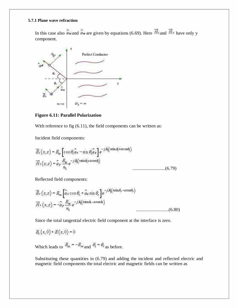
5.7.1 Plane wave refraction

In this case also and are given by equations (6.69). Here and have only y

component.

Figure 6.11: Parallel Polarization

With reference to fig (6.11), the field components can be written as:

Incident field components:

............................(6.79)

Reflected field components:

............................(6.80)

Since the total tangential electric field component at the interface is zero.

Which leads to and as before.

Substituting these quantities in (6.79) and adding the incident and reflected electric and magnetic field components the total electric and magnetic fields can be written as

...........................(6.81)

Once again, we find a standing wave pattern along z for the x and y components of and

, while a non uniform plane wave propagates along

x with a phase velocity given by where . Since, for this

propagating wave, magnetic field is in transverse direction, such waves are called transverse magnetic or TM waves.

Oblique incidence at a plane dielectric interface

We continue our discussion on the behavior of plane waves at an interface; this time we consider a plane dielectric interface. As earlier, we consider the two specific cases, namely parallel and perpendicular polarization.

Fig 6.12: Oblique incidence at a plane dielectric interface

For the case of a plane dielectric interface, an incident wave will be reflected partially and transmitted partially.

In Fig(6.12), corresponds respectively to the angle of incidence, reflection and

transmission.

1. Parallel Polarization

As discussed previously, the incident and reflected field components can be written as

..........................(6.82)

..........................(6.83)

In terms of the reflection coefficient

..........................(6.84)

The transmitted filed can be written in terms of the transmission coefficient T

..........................(6.85)

We can now enforce the continuity of tangential field components at the boundary i.e. z=0

..........................(6.86)

If both and are to be continuous at z=0 for all x , then form the phase matching we

have

We find that

..........................(6.87)

Further, from equations (6.86) and (6.87) we have

..........................(6.88)

or.......................... (6.89)

..........................(6.90)

From equation (6.90) we find that there exists specific angle for

which = 0 such that

or......................... (6.91)

Further, .........................(6.92)

For non magnetic material Using this condition

.........................(6.93)

From equation (6.93), solving for we get

This angle of incidence for which = 0 is called Brewster angle. Since

we are dealing with parallel polarization we represent this angle by so

that

5.7.2 Standing Wave

.........................(6.94)

.........................(6.95)

.........................(6.96)

Using continuity of field components at z=0

.................(6.97)

As in the previous case

.........................(6.98)

Using these conditions we can write

.........................(6.99)

From equation (6.99) the reflection and transmission coefficients for the perpendicular polarization can be computed as

.........................(6.100)

We observe that if = 0 for an angle of incidence

or

or

or......................... (6.101)

We observe if i.e. in this case of non magnetic material

Brewster angle does not exist as the denominator or equation (6.101)

becomes zero. Thus for perpendicular polarization in dielectric media,

there is Brewster angle so that can be made equal to zero.

From our previous discussion we observe that for both polarizations

If

For ;

The incidence angle for which i.e. is called the

critical angle of incidence. If the angle of incidence is larger than total

internal reflection occurs. For such case an evanescent wave exists along

the interface in the x direction (w.r.t. fig (6.12)) that attenuates

exponentially in the normal i.e. z direction. Such waves are tightly bound

to the interface and are called surface waves.