
Coupling of eddy-current and circuit problems
55
Coupling of eddy-current and circuit problems Ana Alonso Rodr´ ıguez*, ALBERTO VALLI*, Rafael V ´ azquez Hern ´ andez** * Department of Mathematics, University of Trento ** Department of Applied Mathematics, University of Santiago de Compostela Coupling of eddy-currentand circuit problems – p.1/28
Transcript of Coupling of eddy-current and circuit problems

Coupling of eddy-currentand circuit problems
Ana Alonso Rodrıguez*, ALBERTO VALLI*, Rafael Vazquez Hernandez**
* Department of Mathematics, University of Trento
** Department of Applied Mathematics, University of Santiago de
Compostela
Coupling of eddy-currentand circuit problems – p.1/28

Time-harmonic eddy-current equations
Starting from Maxwell equations, assuming a sinusoidaldependence on time and disregarding displacementcurrents one obtains the so-called time-harmoniceddy-current problem
curlH − σE = 0 in Ω
curlE + iωµH = 0 in Ω .(1)
Coupling of eddy-currentand circuit problems – p.2/28

Time-harmonic eddy-current equations
Starting from Maxwell equations, assuming a sinusoidaldependence on time and disregarding displacementcurrents one obtains the so-called time-harmoniceddy-current problem
curlH − σE = 0 in Ω
curlE + iωµH = 0 in Ω .(1)
Here
H and E are the magnetic and electric fields,respectively
σ and µ are the electric conductivity and the magneticpermeability, respectively
ω 6= 0 is the frequency.
Coupling of eddy-currentand circuit problems – p.2/28

Time-harmonic eddy-current equations (cont’d)
[As shown in the previous talk, in an insulator one hasσ = 0, therefore E is not uniquely determined in that region(E + ∇ψ is still a solution).Some additional conditions ("gauge" conditions) are thusnecessary: as in the insulator ΩI we have no charges, weimpose
div(ǫE) = 0 in ΩI , (2)
where ǫ is the electric permittivity.]
Coupling of eddy-currentand circuit problems – p.3/28

Geometry
The physical domain Ω ⊂ R3 is a “box", and the conductorΩC is simply-connected with ∂ΩC ∩ ∂Ω = ΓE ∪ ΓJ , where ΓE
and ΓJ are connected and disjoint surfaces on ∂Ω (“electricports"). Notation: Γ = ΩC ∩ ΩI , ∂Ω = ΓE ∪ ΓJ ∪ ΓD,∂ΩC = ΓE ∪ ΓJ ∪ Γ, ∂ΩI = ΓD ∪ Γ.
ΓJ
ΓE
Γ
Ξ
ΓD
Coupling of eddy-currentand circuit problems – p.4/28

Boundary conditions
We will distinguish among three types of boundaryconditions.
Coupling of eddy-currentand circuit problems – p.5/28

Boundary conditions
We will distinguish among three types of boundaryconditions.
Electric (Case A). One imposes E × n = 0 on ∂Ω.
Coupling of eddy-currentand circuit problems – p.5/28

Boundary conditions
We will distinguish among three types of boundaryconditions.
Electric (Case A). One imposes E × n = 0 on ∂Ω.
Magnetic (Case B). One imposes E × n = 0 on ΓE ∪ ΓJ ,H × n = 0 and ǫE · n = 0 on ΓD.
Coupling of eddy-currentand circuit problems – p.5/28

Boundary conditions
We will distinguish among three types of boundaryconditions.
Electric (Case A). One imposes E × n = 0 on ∂Ω.
Magnetic (Case B). One imposes E × n = 0 on ΓE ∪ ΓJ ,H × n = 0 and ǫE · n = 0 on ΓD.
No-flux (Case C) [Bossavit, 2000]. One imposesE × n = 0 on ΓE ∪ ΓJ , µH · n = 0 and ǫE · n = 0 on ΓD.
Coupling of eddy-currentand circuit problems – p.5/28

Voltage and current intensity
When one wants to couple the eddy-current problem with acircuit problem, one has to consider, as the only externaldatum that determines the solution, a voltage V or a currentintensity I0.
Coupling of eddy-currentand circuit problems – p.6/28

Voltage and current intensity
When one wants to couple the eddy-current problem with acircuit problem, one has to consider, as the only externaldatum that determines the solution, a voltage V or a currentintensity I0.
Question:
Coupling of eddy-currentand circuit problems – p.6/28

Voltage and current intensity
When one wants to couple the eddy-current problem with acircuit problem, one has to consider, as the only externaldatum that determines the solution, a voltage V or a currentintensity I0.
Question:
how can we formulate the eddy-current problems whenthe excitation is given by a voltage or by a currentintensity?
This is a delicate point, as eddy-current problems, for thetwo cases A and B, have a unique solution already before avoltage or a current intensity is assigned!
Coupling of eddy-currentand circuit problems – p.6/28

Poynting Theorem (energy balance)
In fact one has:Uniqueness theorem. In the cases A and B for the solutionof the eddy-current problem (1) the magnetic field H in Ωand the electric field EC in ΩC are uniquely determined.[Adding the "gauge" conditions, also the electric field EI inΩI is uniquely determined.]
Coupling of eddy-currentand circuit problems – p.7/28

Poynting Theorem (energy balance)
In fact one has:Uniqueness theorem. In the cases A and B for the solutionof the eddy-current problem (1) the magnetic field H in Ωand the electric field EC in ΩC are uniquely determined.[Adding the "gauge" conditions, also the electric field EI inΩI is uniquely determined.]
Proof. Multiply the Faraday equation by H, integrate in Ωand integrate by parts: it holds
0 =∫
ΩcurlE · H +
∫
ΩiωµH · H
=∫
ΩE · curlH +
∫
ΩiωµH · H +
∫
∂Ωn × E · H .
Remembering that curlHI = 0 in ΩI and replacing curlHC
with σEC , one has the Poynting Theorem (energy balance)
Coupling of eddy-currentand circuit problems – p.7/28

Poynting Theorem (energy balance) (cont’d)
∫
ΩCσEC · EC +
∫
ΩiωµH · H = −
∫
∂Ωn × E · H.
Coupling of eddy-currentand circuit problems – p.8/28

Poynting Theorem (energy balance) (cont’d)
∫
ΩCσEC · EC +
∫
ΩiωµH · H = −
∫
∂Ωn × E · H.
The term on ∂Ω is clearly vanishing in the cases A and B.
Coupling of eddy-currentand circuit problems – p.8/28

Poynting Theorem for the case C
In the case C, instead, since divτ (E × n) = −iωµH · n = 0on ∂Ω, one has
E × n = gradW × n on ∂Ω ,
and therefore
−∫
∂Ωn × E · H = −
∫
∂ΩH × n · gradW
=∫
∂Ωdiv(H× n)W
=∫
∂ΩcurlH · nW = W|ΓJ
∫
ΓJcurlHC · n,
as curlHI = 0 in ΩI , and we have denoted by W|ΓJthe
(constant) value of the potential W on the electric port ΓJ
(whereas W|ΓE= 0).
Coupling of eddy-currentand circuit problems – p.9/28

Poynting Theorem for the case C (cont’d)
In this case a degree of freedom is indeed still free(either the voltage W|ΓJ
, that will be denoted by V , orelse the current intensity
∫
ΓJcurlHC · n in ΩC , that will
be denoted by I0).
Coupling of eddy-currentand circuit problems – p.10/28

Poynting Theorem for the case C (cont’d)
In this case a degree of freedom is indeed still free(either the voltage W|ΓJ
, that will be denoted by V , orelse the current intensity
∫
ΓJcurlHC · n in ΩC , that will
be denoted by I0).
We can thus conclude that the only meaningful boundaryvalue problem is the one with assigned no-flux boundaryconditions: the case C.
Coupling of eddy-currentand circuit problems – p.10/28

The case C: variational formulation
How can we formulate the problem when the voltage orthe current intensity are assigned?
[Alonso Rodríguez, Valli and Vázquez Hernández, 2009][Other approaches: Bíró, Preis, Buchgraber and Ticar,2004; Bermúdez, Rodríguez and Salgado, 2005]
Coupling of eddy-currentand circuit problems – p.11/28

The case C: variational formulation
How can we formulate the problem when the voltage orthe current intensity are assigned?
[Alonso Rodríguez, Valli and Vázquez Hernández, 2009][Other approaches: Bíró, Preis, Buchgraber and Ticar,2004; Bermúdez, Rodríguez and Salgado, 2005]
This orthogonal decomposition result turns out to be useful:each vector function vI can be decomposed as
vI = µ−1
I curl qI + gradψI + αρI ,
where ρI is a harmonic field, namely, it belongs to the space
HµI(ΩI) := vI ∈ (L2(ΩI))
3| curl vI = 0, div(µIvI) = 0,
µIvI · n = 0 on ∂ΩI .
Coupling of eddy-currentand circuit problems – p.11/28

The case C: variational formulation (cont’d)
The harmonic field ρI is known from the data of theproblem, and satisfies
∫
∂ΓJρI · dτ = 1; moreover, if the
vector field vI satisfies curl vI = 0, it follows qI = 0 andtherefore α =
∫
∂ΓJvI · dτ .
Coupling of eddy-currentand circuit problems – p.12/28

The case C: variational formulation (cont’d)
The harmonic field ρI is known from the data of theproblem, and satisfies
∫
∂ΓJρI · dτ = 1; moreover, if the
vector field vI satisfies curl vI = 0, it follows qI = 0 andtherefore α =
∫
∂ΓJvI · dτ .
In particular, setting HI = gradψI + αIρI , from the StokesTheorem one has
I0 =
∫
ΓJ
curlHC · nC =
∫
∂ΓJ
HC · dτ =
∫
∂ΓJ
HI · dτ = αI ,
henceHI = gradψI + I0ρI . (3)
We want to provide a "coupled" variational formulation, interms of EC in ΩC and of HI in ΩI .
Coupling of eddy-currentand circuit problems – p.12/28
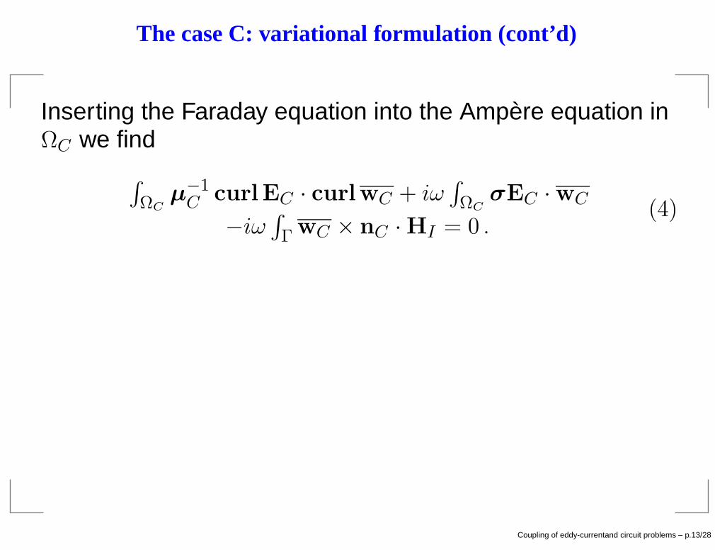
The case C: variational formulation (cont’d)
Inserting the Faraday equation into the Ampère equation inΩC we find
∫
ΩCµ−1
C curlEC · curlwC + iω∫
ΩCσEC · wC
−iω∫
ΓwC × nC · HI = 0 .
(4)
Coupling of eddy-currentand circuit problems – p.13/28

The case C: variational formulation (cont’d)
Inserting the Faraday equation into the Ampère equation inΩC we find
∫
ΩCµ−1
C curlEC · curlwC + iω∫
ΩCσEC · wC
−iω∫
ΓwC × nC · HI = 0 .
(4)
Instead, the Faraday equation in ΩI gives
iω
∫
ΩI
µIHI · gradϕI +
∫
Γ
EC × nC · gradϕI = 0 (5)
and
iω
∫
ΩI
µIHI · ρI +
∫
Γ
EC × nC · ρI = V . (6)
Coupling of eddy-currentand circuit problems – p.13/28

The case C: variational formulation (cont’d)
Here we have to note that∫
ΓDEI × nI · ρI =
∫
ΓDgradW × nI · ρI
=∫
ΓDdivτ (ρI × nI)W + V
∫
∂ΓJρI · dτ = V .
Coupling of eddy-currentand circuit problems – p.14/28

The case C: variational formulation (cont’d)
Here we have to note that∫
ΓDEI × nI · ρI =
∫
ΓDgradW × nI · ρI
=∫
ΓDdivτ (ρI × nI)W + V
∫
∂ΓJρI · dτ = V .
Using (3) in (4), (5) and (6) one has
∫
ΩCµ−1
C curlEC · curlwC + iω∫
ΩCσEC · wC
−iω∫
ΓwC × nC · gradψI − iωI0
∫
ΓwC × nC · ρI = 0
(7)
−iω
∫
Γ
EC×nC ·gradϕI +ω2
∫
ΩI
µI gradψI ·gradϕI = 0 (8)
−iωQ
∫
Γ
EC × nC · ρI + ω2I0Q
∫
ΩI
µIρI · ρI = −iωV Q . (9)
Coupling of eddy-currentand circuit problems – p.14/28

The case C: existence and uniqueness
If V is given, one solves (7), (8), (9) and determines EC ,ψI and I0 (hence HC and HI).
Coupling of eddy-currentand circuit problems – p.15/28

The case C: existence and uniqueness
If V is given, one solves (7), (8), (9) and determines EC ,ψI and I0 (hence HC and HI).
If I0 is given, one solves (7), (8) and determines EC andψI (hence HC and HI); then from (9) one can alsocompute V .
Coupling of eddy-currentand circuit problems – p.15/28

The case C: existence and uniqueness
If V is given, one solves (7), (8), (9) and determines EC ,ψI and I0 (hence HC and HI).
If I0 is given, one solves (7), (8) and determines EC andψI (hence HC and HI); then from (9) one can alsocompute V .
Both problems are well-posed, namely, they have a uniquesolution, since the associated sesquilinear form is coercive(thus one can apply the Lax–Milgram Lemma).
Moreover, it is simple to propose an approximation methodbased on finite elements, of "edge" type for EC in ΩC and of(scalar) nodal type for ψI in ΩI . Convergence is assured bythe Céa Lemma.
Coupling of eddy-currentand circuit problems – p.15/28

The case C: existence and uniqueness
If V is given, one solves (7), (8), (9) and determines EC ,ψI and I0 (hence HC and HI).
If I0 is given, one solves (7), (8) and determines EC andψI (hence HC and HI); then from (9) one can alsocompute V .
Both problems are well-posed, namely, they have a uniquesolution, since the associated sesquilinear form is coercive(thus one can apply the Lax–Milgram Lemma).
Moreover, it is simple to propose an approximation methodbased on finite elements, of "edge" type for EC in ΩC and of(scalar) nodal type for ψI in ΩI . Convergence is assured bythe Céa Lemma. [However, an efficient implementationdemands to replace the harmonic field ρI with an easilycomputable function.]
Coupling of eddy-currentand circuit problems – p.15/28

Physical interpretation
Note: the physical interpretation of equation (9) is that
−
∫
γ
EC · dr + iω
∫
Ξ
µIHI · nΞ = V ,
where γ = ∂Ξ ∩ Γ is oriented from ΓJ to ΓE , and nΞ isdirected in such a way that γ is clockwise oriented withrespect to it.In other words, if it is possible to determine the electric fieldEI in ΩI satisfying the Faraday equation, it follows that
∫
γ∗
EI · dr = V ,
where γ∗ = ∂Ξ ∩ ΓD is oriented from ΓE to ΓJ : hence (9) isindeed determining the voltage drop between the electricports.
Coupling of eddy-currentand circuit problems – p.16/28

Physical interpretation (cont’d)
This explains from another point of view why, when thesource is a voltage drop or a current intensity, it is notpossible to assume the electric boundary conditionsE × n = 0 on ∂Ω.
Coupling of eddy-currentand circuit problems – p.17/28

Physical interpretation (cont’d)
This explains from another point of view why, when thesource is a voltage drop or a current intensity, it is notpossible to assume the electric boundary conditionsE × n = 0 on ∂Ω.In fact, in that case one would have
∫
γ∗
EI · dr = 0 ,
hence from (9)
iω∫
ΞµIHI · nΞ = V +
∫
γ EC · dr = V +∫
γ∪γ∗
E · dr
= V +∫
∂ΞE · dr ,
with ∂Ξ clockwise oriented with respect nΞ: due to the termV the Faraday equation would be violated on Ξ!
Coupling of eddy-currentand circuit problems – p.17/28

Numerical results for the Case C
Coming back to the case C and to its variational formulation(7), (8), (9), we use edge finite elements of the lowestdegree (a + b × x in each element) for approximating EC ,and scalar piecewise-linear elements for approximating ψI .
Coupling of eddy-currentand circuit problems – p.18/28

Numerical results for the Case C
Coming back to the case C and to its variational formulation(7), (8), (9), we use edge finite elements of the lowestdegree (a + b × x in each element) for approximating EC ,and scalar piecewise-linear elements for approximating ψI .
The problem description is the following: the conductor ΩC
and the whole domain Ω are two coaxial cylinders of radiusRC and RD, respectively, and height L. Assuming that σ
and µ are scalar constants, the exact solution for anassigned current intensity I0 is known (through suitableBessel functions), and also the basis function ρI is known,thus from (9) one easily computes the voltage V , too.
Coupling of eddy-currentand circuit problems – p.18/28

Numerical results for the Case C (cont’d)
We have the following data:
RC = 0.25 m
RD = 0.5 m
L = 0.25 m
σ = 151565.8 S/m
µ = 4π × 10−7 H/m
ω = 2π × 50 rad/s
and
I0 = 104 A or V = 0.08979 + 0.14680i
[the voltage corresponds to the current intensity I0 = 104 A].
Coupling of eddy-currentand circuit problems – p.19/28

Numerical results for the Case C (cont’d)
The relative errors (for EC in H(curl; ΩC) and for HI inL2(ΩI)) with respect to the number of degrees of freedomare given by:
Coupling of eddy-currentand circuit problems – p.20/28
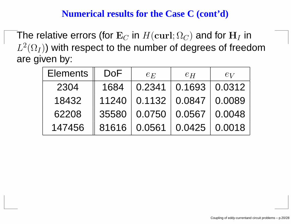
Numerical results for the Case C (cont’d)
The relative errors (for EC in H(curl; ΩC) and for HI inL2(ΩI)) with respect to the number of degrees of freedomare given by:
Elements DoF eE eH eV
2304 1684 0.2341 0.1693 0.031218432 11240 0.1132 0.0847 0.008962208 35580 0.0750 0.0567 0.0048147456 81616 0.0561 0.0425 0.0018
Elements DoF eE eH eI0
2304 1685 0.2336 0.1685 0.027418432 11241 0.1132 0.0847 0.008562208 35581 0.0750 0.0566 0.0041147456 81617 0.0561 0.0425 0.0024
Coupling of eddy-currentand circuit problems – p.20/28

Numerical results for the Case C (cont’d)
On a graph: for assigned current intensity
103
104
105
10−4
10−3
10−2
10−1
100
Number of d.o.f.
Rel
ativ
e er
rors
Rel. error EC
Rel. error HD
Rel. error Vy = Ch
y=Ch2
Coupling of eddy-currentand circuit problems – p.21/28
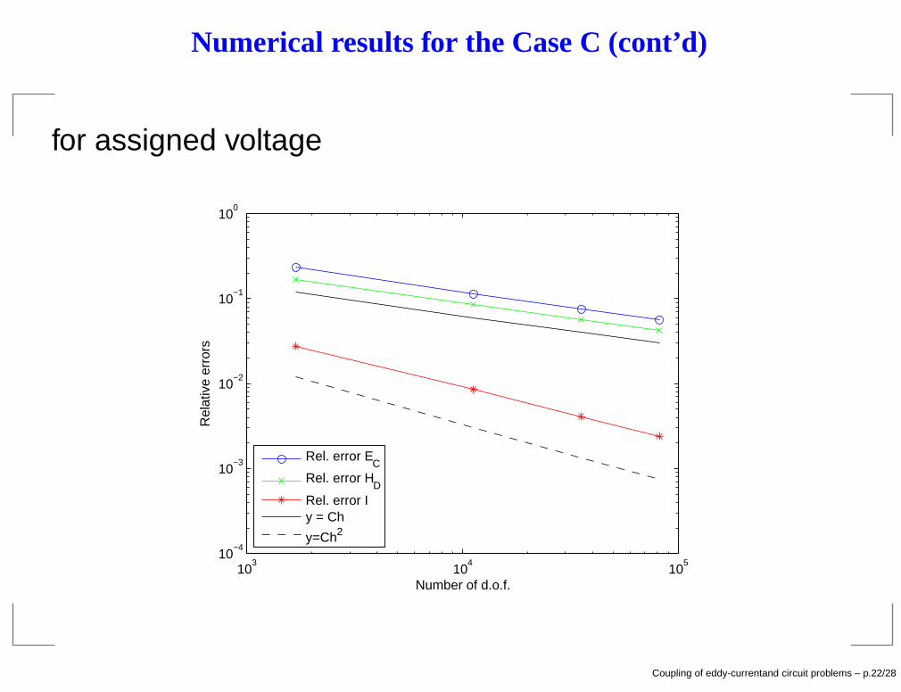
Numerical results for the Case C (cont’d)
for assigned voltage
103
104
105
10−4
10−3
10−2
10−1
100
Number of d.o.f.
Rel
ativ
e er
rors
Rel. error EC
Rel. error HD
Rel. error Iy = Ch
y=Ch2
Coupling of eddy-currentand circuit problems – p.22/28

Numerical results for the Case C (cont’d)
A more realistic problem, considered by Bermúdez,Rodríguez and Salgado, 2005, is that of a cylindricalelectric furnace with three electrodes ELSA [dimensions:furnace height 2 m; furnace diameter 8.88 m; electrodeheight 1.25 m; electrode diameter 1 m; distance of thecenter of the electrode from the wall 3 m].
Coupling of eddy-currentand circuit problems – p.23/28

Numerical results for the Case C (cont’d)
A more realistic problem, considered by Bermúdez,Rodríguez and Salgado, 2005, is that of a cylindricalelectric furnace with three electrodes ELSA [dimensions:furnace height 2 m; furnace diameter 8.88 m; electrodeheight 1.25 m; electrode diameter 1 m; distance of thecenter of the electrode from the wall 3 m].The three electrodes ELSA are constituted by a graphitecore of 0.4 m of diameter, and by an outer part ofSöderberg paste. The electric current enters the electrodesthrough horizontal copper bars of rectangular section (0.07m×0.25 m), connecting the top of the electrode with theexternal boundary.
Coupling of eddy-currentand circuit problems – p.23/28

Numerical results for the Case C (cont’d)
A more realistic problem, considered by Bermúdez,Rodríguez and Salgado, 2005, is that of a cylindricalelectric furnace with three electrodes ELSA [dimensions:furnace height 2 m; furnace diameter 8.88 m; electrodeheight 1.25 m; electrode diameter 1 m; distance of thecenter of the electrode from the wall 3 m].The three electrodes ELSA are constituted by a graphitecore of 0.4 m of diameter, and by an outer part ofSöderberg paste. The electric current enters the electrodesthrough horizontal copper bars of rectangular section (0.07m×0.25 m), connecting the top of the electrode with theexternal boundary.Data: σ = 106 S/m for graphite, σ = 104 S/m for Söderbergpaste, σ = 5 × 10⁶ S/m for copper, µ = 4π × 10−7 H/m,ω = 2π × 50 rad/s, I0 = 7 × 10⁴ A for each electrode.
Coupling of eddy-currentand circuit problems – p.23/28

Numerical results for the Case C (cont’d)
The value of the magnetic "potential" in the insulator: themagnetic field is the gradient of the represented function(not taking into account the jump surfaces).
Coupling of eddy-currentand circuit problems – p.24/28

Numerical results for the Case C (cont’d)
The magnitude of the current density σEC on a horizontalsection of one electrode.
Coupling of eddy-currentand circuit problems – p.25/28

Numerical results for the Case C (cont’d)
The magnitude of the current density σEC on a verticalsection of one electrode.
Coupling of eddy-currentand circuit problems – p.26/28

References
A. Alonso Rodríguez, A. Valli and R. Vázquez Hernández:A formulation of the eddy-current problem in the presenceof electric ports. Numer. Math., 113 (2009), 643–672.
A. Bermúdez, R. Rodríguez and P. Salgado: Numericalsolution of eddy-current problems in bounded domainsusing realistic boundary conditions. Comput. Methods Appl.Mech. Engrg., 194 (2005), 411–426.
O. Bíró, K. Preis, G. Buchgraber and I. Ticar: Voltage-drivencoils in finite-element formulations using a current vectorand a magnetic scalar potential, IEEE Trans. Magn., 40(2004), 1286–1289.
A. Bossavit: Most general ‘non-local’ boundary conditionsfor the Maxwell equations in a bounded region. COMPEL,19 (2000), 239—245.
Coupling of eddy-currentand circuit problems – p.27/28

Additional references
A. Alonso Rodríguez and A. Valli: Voltage and currentexcitation for time-harmonic eddy-current problem. SIAM J.Appl. Math., 68 (2008), 1477–1494.
P. Dular, C. Geuzaine and W. Legros: A natural method forcoupling magnetodynamic H-formulations and circuitsequations. IEEE Trans. Magn., 35 (1999), 1626–1629.
R. Hiptmair and O. Sterz: Current and voltage excitationsfor the eddy current model. Int. J. Numer. Modelling, 18(2005), 1–21.
J. Rappaz, M. Swierkosz and C.Trophime: Un modèlemathématique et numérique pour un logiciel de simulationtridimensionnelle d’induction électromagnétique. Report05.99, Département de Mathématiques, ÉcolePolytechnique Fédérale de Lausanne, 1999.
Coupling of eddy-currentand circuit problems – p.28/28


![coupling circuit - arXiv · coupling (J12 (w c;of f) = 0), as well as the static ZZ coupling xZZ when two qubits are detuned in dispersive regime [13]. Now we apply a ux to the tunable](https://static.fdocuments.in/doc/165x107/5f7895986ae1bd225c41e5d4/coupling-circuit-arxiv-coupling-j12-w-cof-f-0-as-well-as-the-static-zz.jpg)