Count regression gmodels for novel NIDA ‘NIDA ‘process phenotypes‘phenotypesCPDD Methods WorkshopS d 10 J 2012Sunday, 10 June 2012Palm Springs, California

i hJim AnthonyProfessor of Epidemiology & BiostatisticsCollege of Human MedicineMichigan State University Ask me about our open postdoctoral g yEast Lansing, Michigan 48823janthony@msu.edu

(and predoctoral) NIDA research training fellowships for US citizens and green card holders.

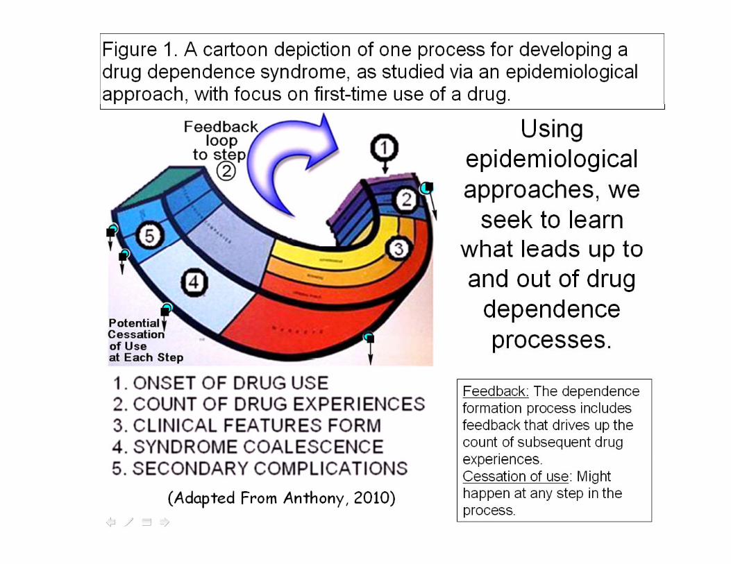
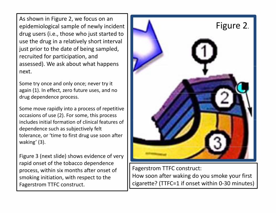
As shown in Figure 2, we focus on an epidemiological sample of newly incident drug users (i.e., those who just started to 

h d i l i l h i l

Figure 2. use the drug in a relatively short interval just prior to the date of being sampled, recruited for participation, and assessed). We ask about what happens ) ppnext.

Some try once and only once; never try it again (1). In effect, zero future uses, and no drug dependence process.

Some move rapidly into a process of repetitive occasions of use (2). For some, this process 

l d l f f l l f fincludes initial formation of clinical features of dependence such as subjectively felt tolerance, or ‘time to first drug use soon after waking’ (3).

Figure 3 (next slide) shows evidence of very rapid onset of the tobacco dependence process, within six months after onset of  Fagerstrom TTFC construct:

f ki d k fismoking initiation, with respect to the Fagerstrom TTFC construct.

How soon after waking do you smoke your first cigarette? (TTFC=1 if onset within 0‐30 minutes)

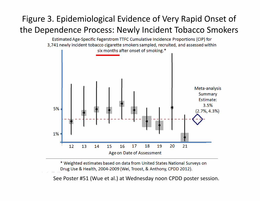
Figure 3. Epidemiological Evidence of Very Rapid Onset of the Dependence Process: Newly Incident Tobacco Smokers

See Poster #51 (Wue et al.) at Wednesday noon CPDD poster session.

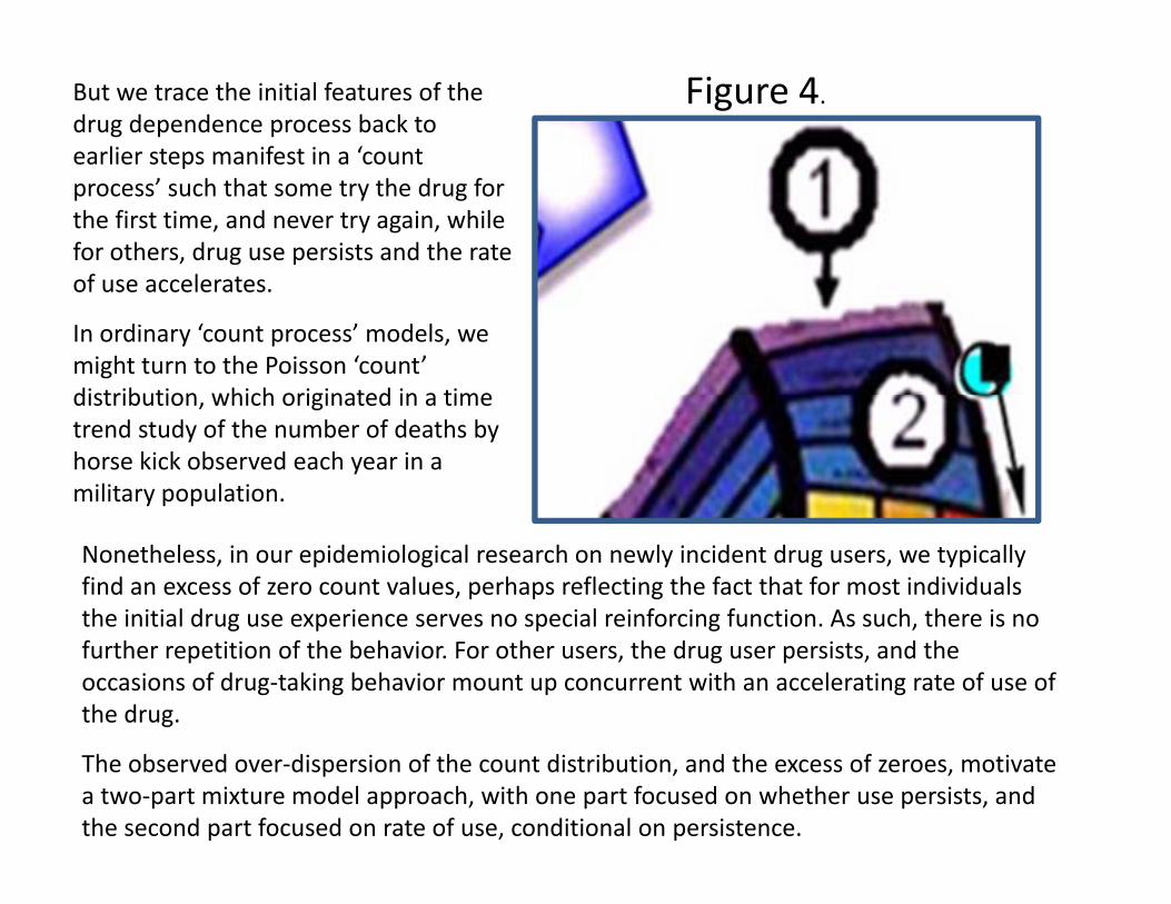
But we trace the initial features of the drug dependence process back to earlier steps manifest in a ‘count 

Figure 4. p

process’ such that some try the drug for the first time, and never try again, while for others, drug use persists and the rate of use acceleratesof use accelerates.

In ordinary ‘count process’ models, we might turn to the Poisson ‘count’ distribution which originated in a timedistribution, which originated in a time trend study of the number of deaths by horse kick observed each year in a military population.

Nonetheless, in our epidemiological research on newly incident drug users, we typically find an excess of zero count values, perhaps reflecting the fact that for most individuals the initial drug use experience serves no special reinforcing function As such there is nothe initial drug use experience serves no special reinforcing function. As such, there is no further repetition of the behavior. For other users, the drug user persists, and the occasions of drug‐taking behavior mount up concurrent with an accelerating rate of use of the drug.

The observed over‐dispersion of the count distribution, and the excess of zeroes, motivate a two‐part mixture model approach, with one part focused on whether use persists, and the second part focused on rate of use, conditional on persistence. 

In our research group at Michigan State University, David Barondess has been the y,leader of our work to study this count process soon after onset of tobacco cigarette smoking which follows acigarette smoking, which follows a chance to try tobacco.

’ll f h ’ kI’ll present some of the group’s work to illustrate our conceptualization of a ‘novel phenotype’ that can be observed p ypearly in the process of drug involvement. This ‘count process phenotype’ has two facets One facet involves persistencefacets. One facet involves persistence versus non‐persistence of drug use. The other facet involves estimation of the 

f d di i lrate of drug use, conditional on persistence of use.

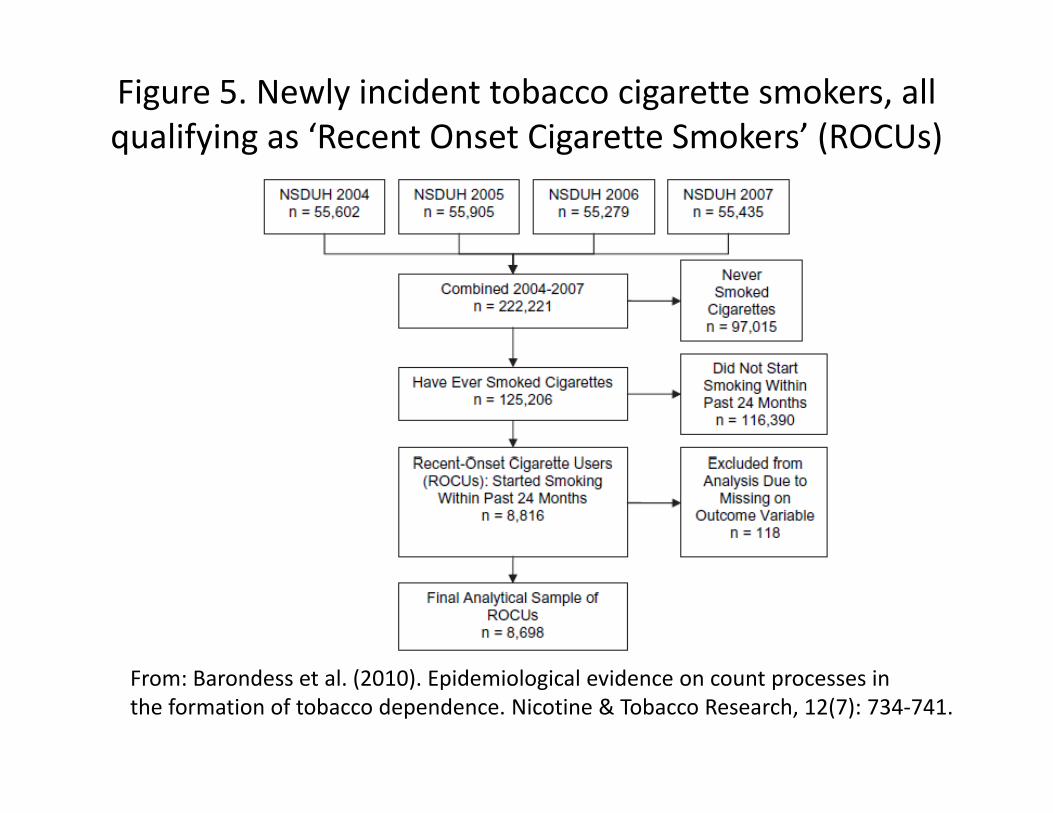
Figure 5. Newly incident tobacco cigarette smokers, all qualifying as ‘Recent Onset Cigarette Smokers’ (ROCUs)q y g g ( )

From: Barondess et al. (2010). Epidemiological evidence on count processes inthe formation of tobacco dependence. Nicotine & Tobacco Research, 12(7): 734‐741.

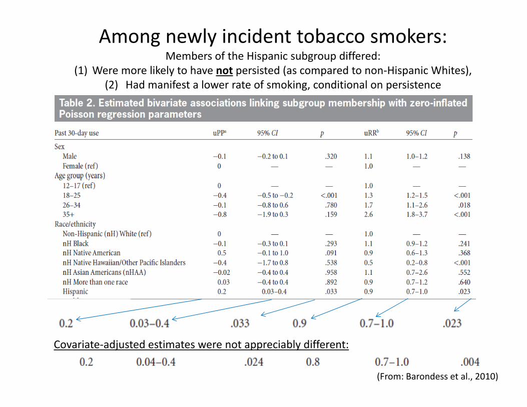
Among newly incident tobacco smokers:Members of the Hispanic subgroup differed:

(1) Were more likely to have not persisted (as compared to non‐Hispanic Whites),( ) y p ( p p ),(2) Had manifest a lower rate of smoking, conditional on persistence

Covariate‐adjusted estimates were not appreciably different:

(From: Barondess et al., 2010)

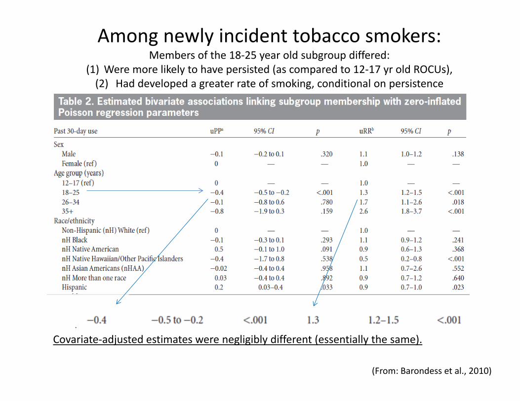
Among newly incident tobacco smokers:Members of the 18‐25 year old subgroup differed:

(1) Were more likely to have persisted (as compared to 12‐17 yr old ROCUs),( ) y p ( p y ),(2) Had developed a greater rate of smoking, conditional on persistence

Covariate‐adjusted estimates were negligibly different (essentially the same).

(From: Barondess et al., 2010)

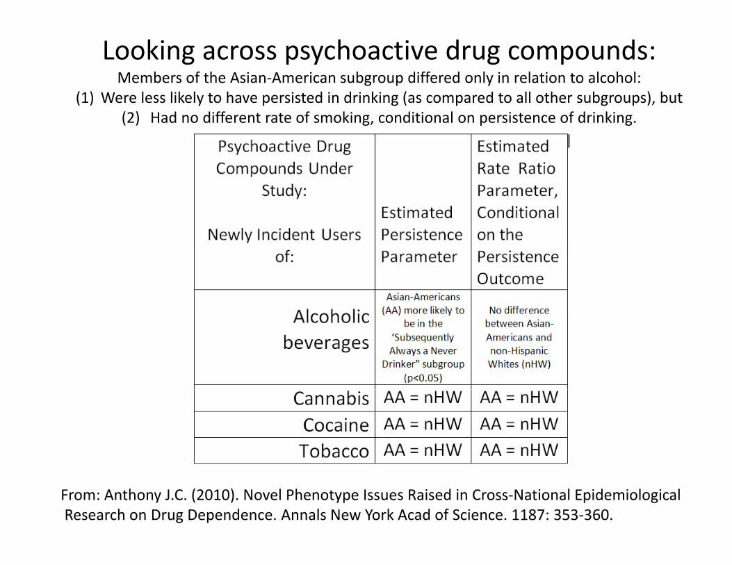
Looking across psychoactive drug compounds:Members of the Asian‐American subgroup differed only in relation to alcohol:

(1) Were less likely to have persisted in drinking (as compared to all other subgroups), but( ) y p g ( p g p ),(2) Had no different rate of smoking, conditional on persistence of drinking.

From: Anthony J.C. (2010). Novel Phenotype Issues Raised in Cross‐National EpidemiologicalResearch on Drug Dependence. Annals New York Acad of Science. 1187: 353‐360.

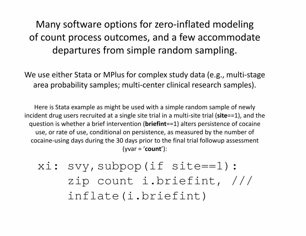
Many software options for zero‐inflated modelingof count process outcomes, and a few accommodate

departures from simple random sampling.

We use either Stata or MPlus for complex study data (e g multi stageWe use either Stata or MPlus for complex study data (e.g., multi‐stage area probability samples; multi‐center clinical research samples).

Here is Stata example as might be used with a simple random sample of newly incident drug users recruited at a single site trial in a multi‐site trial (site==1), and the question is whether a brief intervention (briefint==1) alters persistence of cocaine use or rate of use conditional on persistence as measured by the number of

i b (if it 1)

use, or rate of use, conditional on persistence, as measured by the number of cocaine‐using days during the 30 days prior to the final trial followup assessment 

(yvar = ‘count’):

xi: svy,subpop(if site==1): zip count i.briefint, ///i fl t (i b i fi t)inflate(i.briefint)

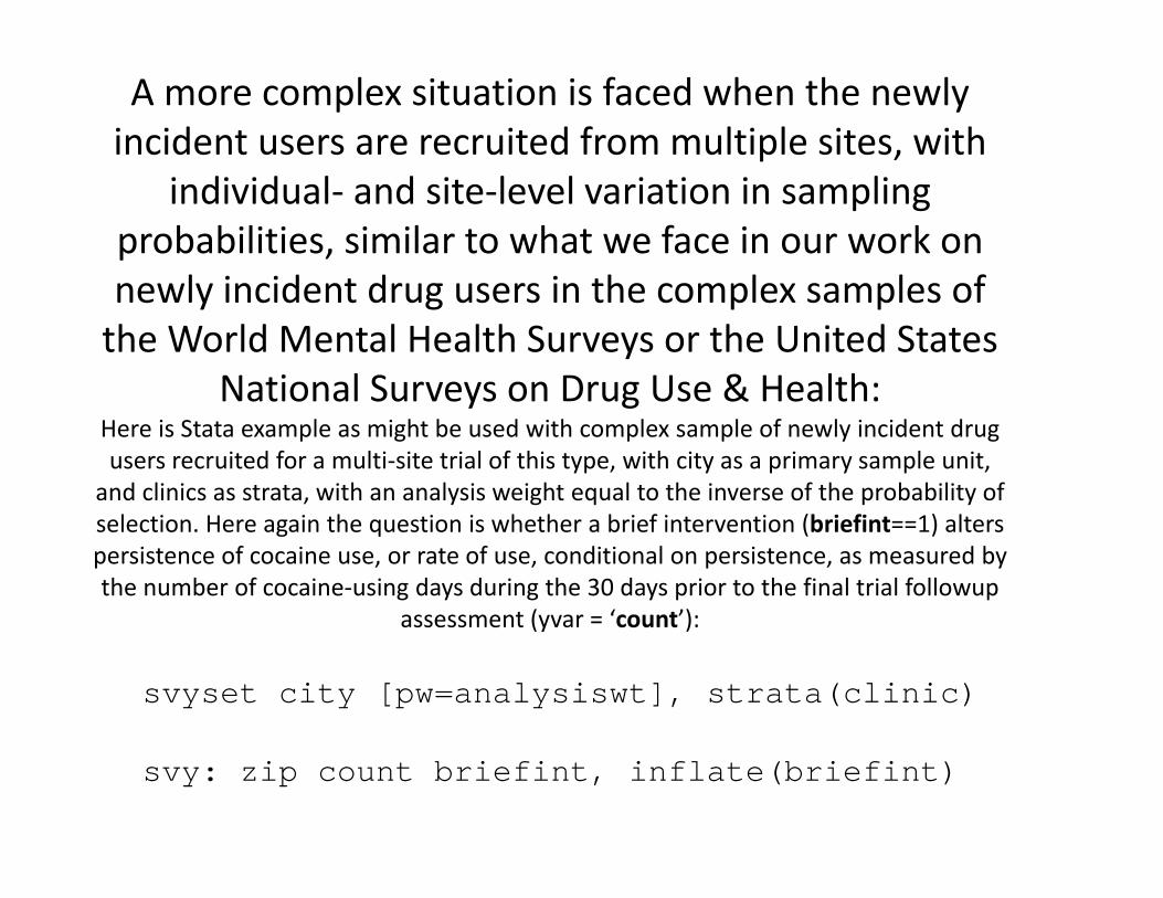
A more complex situation is faced when the newly incident users are recruited from multiple sites, with 

individual‐ and site‐level variation in sampling probabilities, similar to what we face in our work on 

l i id t d i th l l fnewly incident drug users in the complex samples of the World Mental Health Surveys or the United States 

National Surveys on Drug Use & Health:National Surveys on Drug Use & Health:Here is Stata example as might be used with complex sample of newly incident drug users recruited for a multi‐site trial of this type, with city as a primary sample unit, 

and clinics as strata, with an analysis weight equal to the inverse of the probability of selection. Here again the question is whether a brief intervention (briefint==1) alters persistence of cocaine use, or rate of use, conditional on persistence, as measured by the number of cocaine‐using days during the 30 days prior to the final trial followup 

assessment (yvar = ‘count’):

svyset city [pw=analysiswt], strata(clinic)

assessment (yvar =  count ):

svy: zip count briefint, inflate(briefint)

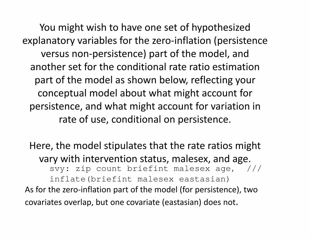
You might wish to have one set of hypothesized explanatory variables for the zero‐inflation (persistence p y (p

versus non‐persistence) part of the model, and another set for the conditional rate ratio estimation part of the model as shown below, reflecting your conceptual model about what might account for 

persistence and what might account for variation inpersistence, and what might account for variation in rate of use, conditional on persistence.

Here, the model stipulates that the rate ratios might vary with intervention status, malesex, and age.

svy: zip count briefint malesex age, ///inflate(briefint malesex eastasian)

As for the zero‐inflation part of the model (for persistence), two covariates overlap, but one covariate (eastasian) does not.

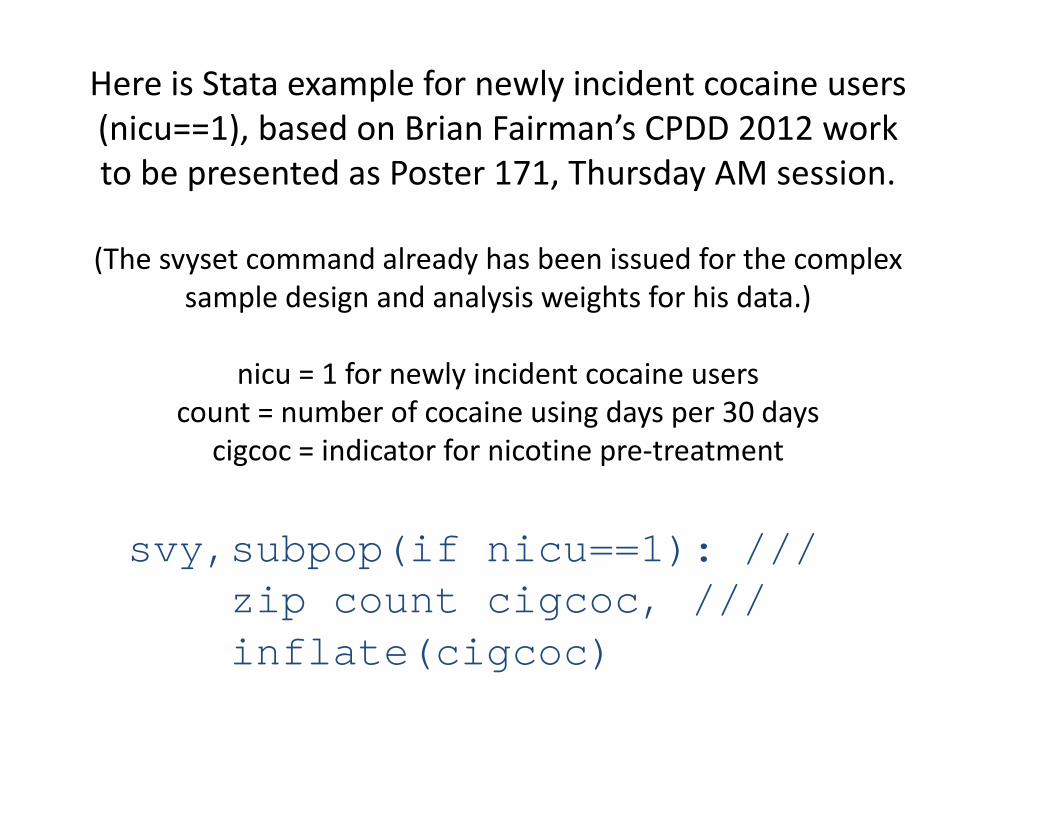
Here is Stata example for newly incident cocaine users (nicu==1), based on Brian Fairman’s CPDD 2012 work to be presented as Poster 171, Thursday AM session.

(Th t d l d h b i d f th l(The svyset command already has been issued for the complex sample design and analysis weights for his data.)

nicu = 1 for newly incident cocaine userscount = number of cocaine using days per 30 days

cigcoc = indicator for nicotine pre‐treatment

svy,subpop(if nicu==1): ///

cigcoc   indicator for nicotine pre treatment

svy,subpop(if nicu 1): /// zip count cigcoc, ///inflate(cigcoc)inflate(cigcoc)

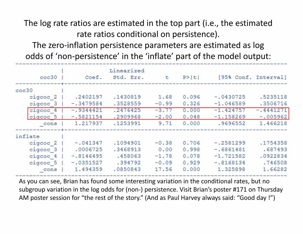
The log rate ratios are estimated in the top part (i.e., the estimated rate ratios conditional on persistence).

Th i fl ti i t t ti t d lThe zero‐inflation persistence parameters are estimated as log odds of ‘non‐persistence’ in the ‘inflate’ part of the model output:

As you can see, Brian has found some interesting variation in the conditional rates, but no subgroup variation in the log odds for (non‐) persistence. Visit Brian’s poster #171 on Thursdaysubgroup variation in the log odds for (non ) persistence. Visit Brian s poster #171 on Thursday AM poster session for “the rest of the story.” (And as Paul Harvey always said: “Good day !”)

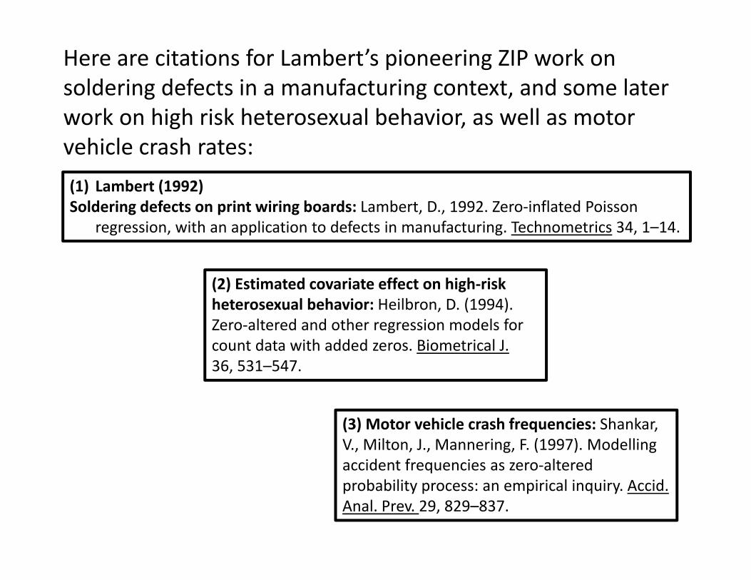
Here are citations for Lambert’s pioneering ZIP work on soldering defects in a manufacturing context, and some later 

( ) b ( )

work on high risk heterosexual behavior, as well as motor vehicle crash rates:(1) Lambert (1992)Soldering defects on print wiring boards: Lambert, D., 1992. Zero‐inflated Poisson 

regression, with an application to defects in manufacturing. Technometrics 34, 1–14.

(2) Estimated covariate effect on high‐risk heterosexual behavior: Heilbron, D. (1994). Zero‐altered and other regression models forZero altered and other regression models for count data with added zeros. Biometrical J.36, 531–547.

(3) Motor vehicle crash frequencies: Shankar, V., Milton, J., Mannering, F. (1997). Modellingaccident frequencies as zero‐altered qprobability process: an empirical inquiry. Accid. Anal. Prev. 29, 829–837.

THANK YOU!! (ALMOST TIME FOR SWIMMING !!!)