This paper can be downloaded without charge at:

The Fondazione Eni Enrico Mattei Note di Lavoro Series Index: http://www.feem.it/Feem/Pub/Publications/WPapers/default.htm

Social Science Research Network Electronic Paper Collection:

http://ssrn.com/abstract=951455

The opinions expressed in this paper do not necessarily reflect the position of Fondazione Eni Enrico Mattei

Corso Magenta, 63, 20123 Milano (I), web site: www.feem.it, e-mail: working.papers@feem.it

Costs of Reducing Greenhouse Gas Emissions: A Case Study of

India’s Power Generation Sector Manish Gupta

NOTA DI LAVORO 147.2006

DECEMBER 2006 CCMP – Climate Change Modelling and Policy

Manish Gupta, National Institute of Public Finance and Policy

Costs of Reducing Greenhouse Gas Emissions: A Case Study of India’s Power Generation Sector

Summary If India were to participate in any international effort towards mitigating CO2 emissions, the power sector which is one of the largest emitters of CO2 in the country would be required to play a major role. In this context the study estimates the marginal abatement costs, which correspond to the costs incurred by the power plants to reduce one unit of CO2 from the current level. The study uses an output distance function approach and its duality with the revenue function to derive these costs for a sample of thermal plants in India. Two sets of exercises have been undertaken. The average shadow prices of CO2 for the sample of thermal plants for the period 1991-92 to 1999-2000 was estimated to be respectively Rs.3380.59 and Rs.2401.99 per ton for the two models. These shadow prices can be used for designing environmental policies and market-based instruments for controlling pollution in the power sector in India. Keywords: Marginal Abatement Costs, Distance Function, CO2 Emissions, Shadow Prices, Power Generation Sector JEL Classification: Q40

Address for correspondence: Manish Gupta National Institute of Public Finance and Policy 18/2 Satsang Vihar Marg Special Institutional Area (Near JNU) New Delhi 110 067 India Phone: 011 26563305, 011 26569303 (Office) E-mail: manish@nipfp.org.in

2

1. Introduction

Issues concerning greenhouse gas (GHG) emission and global warming have received a

great deal of attention in the recent years. As per the Kyoto Protocol signed in 1997, the

industrialised countries, which have historically been mostly responsible for increase in GHG

concentration, agreed to reduce the flow of their GHG emission by 5.2 percent below the level

prevailing in 1990. While the developing countries do not yet have any binding commitment,

there is a realization that large developing countries such as China and India need to take some

action in this regard since they are among the large contributors to incremental emissions. Any

commitment by India towards reducing emissions would mean that all the sectors in the

economy would have to make efforts for reducing their respective GHG emissions so that the

national emission targets are met.

Power sector in India is one of the largest emitters of carbon dioxide (CO2) in the country

accounting for about 35.53 percent of the total CO2 emissions in the year 2001-02 (see Table 1).

The main reason for such a high share is its heavy reliance upon coal. About 81.7 percent of the

total power generation by the utilities in the country in the year 2000-01 was from coal (GOI,

2002). In addition, the coal burnt in the thermal power plants in the country is of inferior quality

thereby resulting in an even higher level of emissions.1 Thus, in near future if India were to

participate in any international effort towards mitigating CO2 emissions, the power sector, which

is one of the largest emitter of carbon dioxide in the country, would be required to play a major

role.

In this context the present study analyses the potential costs imposed on the coal fired

thermal power plants, one of the main sources of CO2 emissions in India, by the implementation

of environmental regulation. More specifically the study aims to estimate the marginal abatement

costs, which corresponds to the costs incurred by the power plants to reduce one unit of carbon

dioxide from the current level. The present exercise, therefore, seeks to derive the ‘shadow

prices’ of reducing carbon dioxide emissions generated by the thermal plants in India. It thus

attempts to provide an answer to the question: how much does it cost the thermal plants in India

to reduce CO2 emission in terms of foregone output or revenue? These estimates are expected to

help in formulating environmental policies. The marginal abatement costs thus obtained would

1 Coal used in coal-fired power plants in India has a low calorific value (around 3,500 Kcal/kg) and a high ash content (as high as 45%).

3

provide guidance on whether the current regulation on pollution satisfies the cost-effectiveness

criterion which is based on the principle of marginal abatement costs be equal across individual

power plants (Baumol and Oates, 1988). It is being recognized by the developed world that the

marketable emission permit system is a more efficient way of regulating pollution. The unit price

of a marketable emission permit would be equivalent to the derived marginal abatement costs

(Baumol and Oates, 1988; Titenberg, 1985). Consequently, these estimates of marginal

abatement cost could be used to predict the price level of emission permits to be introduced.

Table 1: Carbon dioxide Emissions in India (mn t CO2)

Year Aggregate Emissions Power Sector

Emissions

Share of Power Sector in Total

Emission (%)

80-81 244.71 68.06 27.81

85-86 342.22 105.09 30.71

90-91 481.70 170.42 35.38

95-96 632.08 237.98 37.65

96-97 676.80 250.49 37.01

97-98 704.05 269.81 38.32

98-99 632.41 185.33 29.31

99-00 682.78 219.98 32.22

00-01 736.49 242.98 32.99

01-02 698.76 248.24 35.53

Source: Derived from Energy Balance Table using TEDDY (various years) and IPCC (1995).

Theoretical framework of the study is based on production theory and in particular on the

distance function approach. The distance function (also known as the gauge function,

transformation function, or deflation function) identifies a boundary or a frontier technology,

which contains all observation on one side of the frontier and minimises a suitable measure of

the total distance of all observations from the frontier. Although the basic ingredients of the

theoretical framework on which the distance function is based was known long ago owing to the

works of Debreu (1951), Malmquist (1953), and Shephard (1953, 1970), its application became

popular only in the recent years by the works of Rolf Färe, Shawna Grosskopf and others. The

methodology based on distance function framework was first developed by Färe et al.(1993) and

applied by Coggins and Swinton (1996) to the US coal burning utilities. Hetemäki (1996), Kwon

4

and Yun (1999), Murty and Kumar (2002) etc. have also used the technique to derive the shadow

prices of reducing the undesirable outputs. The main advantage of using the distance function

approach over the conventional ones i.e., the production, cost, revenue and profit function is its

computation requiring only quantity data. This feature is of particular importance in the field of

environment economics since price data related to environmental compliance costs are often not

available or are unreliable.

The present study uses the output distance function and its duality with the revenue

function to derive the marginal abatement costs or the shadow prices of reducing CO2 emissions

for a sample of coal fired thermal power plants in India. The remainder of the paper is organized

as follows: the next section provides a theoretical model for estimating the marginal abatement

costs. It also describes the methodology for deriving marginal abatement costs using an output

distance function approach. Section 3 highlights the procedure for the empirical estimation of the

model while Section 4 provides information on the data used and also discusses the estimation

procedure. The estimated results are presented in Section 5. The final Section 6 concludes by

summarizing the main results of the study.

2. Theoretical Model

The conventional production function is defined as the maximum output that can be

produced from a given vector of inputs. The distance function generalizes this concept to a multi-

output case and describes how far an output vector is from the boundary of the representative

output set. We can define the output distance function in terms of the output set P(x). Suppose

that a producer employs the vector of inputs NRx +∈ to produce the vector of outputs M

Ry +∈ ,

where MNRR ++ , are non-negative N and M dimensional Euclidean spaces, respectively. The plant

technology captures the relationship between the inputs and outputs and is described by the

output set )(xP . The output set P(x) denotes all output vectors that are technically feasible for

any given input vector x, i.e.,

}:{)()( yproducecanxRyxPi M

+∈=KK

The output set is assumed to satisfy certain axioms, the details of which can be seen in Färe

(1988). The output distance function is defined on the output set P(x) as

No RxxPyyxDii +∈∀∈>= )}()/(:0{min),()( θθ

θKK

5

The above equation measures the largest radial expansion of the output vector y, for a given

input vector x, that is consistent with y belonging to P(x). The value of the output distance

function must be less than or equal to one for any feasible output. The axioms regarding the

output set P(x) impose a set of properties2 on the output distance function some of which are as

follows:

1. ,0),0( ≥∞+= yforyDo i.e., there is no free lunch. To produce outputs one requires inputs.

2. ,0)0,( No RinxallforxD += i.e., inaction is possible. No output is possible from positive

inputs.

3. ),,(),'(' yxDyxDthatimpliesxx oo ≤≥ i.e., more the inputs the less efficient would the

production be.

4. ,0),(),( >= µµµ foryxDyxD oo i.e., positive linear homogeneity.

5. ),( yxDo is convex in y.

Of particular interest for our purpose is the disposability properties of the technology

with respect to the output, especially the undesirable outputs. We assume that such outputs are

weakly disposable i.e., a reduction in the undesirable outputs can only be achieved by

simultaneously reducing some of the desirable outputs. We also assume that the desirable outputs

are strongly disposable i.e., it is possible to reduce the desirable outputs without actually

reducing the undesirable outputs. In other words the outputs are weakly disposable if

)(],1,0[)( xPythenandxPy ∈∈∈ θθ ; and strongly disposable if we have

)()( xPimpliesxPy ∈∈≤ νν .

Let r = (r1, r2, …… rM) denote the output price vector. Using the output set concept we

can now define the revenue function in the lines of Shephard (1970), and Färe and Primont

(1995) as

)](:[max),()( xPyryrxRiiiy

∈=KK

The revenue function describes the maximum revenue that can be obtained from a given

technology at the output price r. The revenue function, like the distance function, completely

describes the production technology. Shephard (1970) showed that the revenue function and the

output distance function are dual to one another. So,

2 For detailed descriptions of these properties refer to Färe (1988).

6

]1),(:[max),()( ≤= yxDryrxRiv oy

KK

]1),(:[max),()( ≤= rxRryyxDvr

oKK

Thus the revenue function can be derived from the output distance function by maximising

revenue over output quantities, and the output distance function can be derived by maximising

the revenue function over output prices. This duality between the output distance function and

the revenue function can be used to derive the shadow prices of the outputs. These are relative

output shadow prices and in order to obtain absolute shadow prices additional information

regarding the revenue is required (Färe et al 1993). In order to derive the shadow prices of

outputs we assume that both the revenue and distance functions are differentiable. We follow the

methodology used by Färe et al (1993) to derive the shadow price of the undesirable output. Let

m′ output be the undesirable output. In order to derive the shadow price of the undesirable

output it is assumed that the price of at least one of the desirable output (say, the mth output) is

known and is equal to its shadow price, omr . Then the absolute shadow price mr ′ of the m′ output

can be computed as

m

o

m

o

omm

yyxD

yyxD

rrvi

∂∂

∂∂

∗= ′′ ),(

),(

)( KK

As can be seen from equation (vi), the shadow price of the m′ output (the undesirable

output) is given by the product of the market price of the mth output (the desirable output) and the

marginal rate of transformation. This, in turn, is equivalent to the value of the foregone desirable

output associated with the reduction in one unit of the undesirable output. In the above equation

the ratio of the output shadow prices reflects the relative opportunity cost of the output in terms

of the revenue foregone. In other words, it is equivalent to the marginal rate of transformation

between the outputs. Thus the shadow prices reflect the trade-off between the desirable and

undesirable outputs at the actual mix of outputs. Derivation of the shadow prices of undesirable

output as given by equation (vi) is based on the assumption that the production is occurring at the

frontier of the output set. But if the production firms lie within the output set and not on the

frontier (i.e., for such firms the value of the output distance function is less than one) then there

might be some problem in estimating the shadow prices. To resolve the problem of estimating

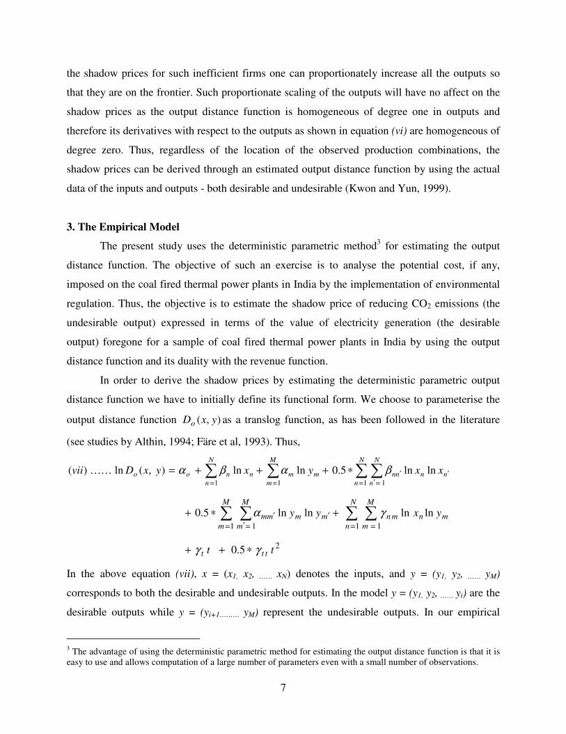
7

the shadow prices for such inefficient firms one can proportionately increase all the outputs so

that they are on the frontier. Such proportionate scaling of the outputs will have no affect on the

shadow prices as the output distance function is homogeneous of degree one in outputs and

therefore its derivatives with respect to the outputs as shown in equation (vi) are homogeneous of

degree zero. Thus, regardless of the location of the observed production combinations, the

shadow prices can be derived through an estimated output distance function by using the actual

data of the inputs and outputs - both desirable and undesirable (Kwon and Yun, 1999).

3. The Empirical Model

The present study uses the deterministic parametric method3 for estimating the output

distance function. The objective of such an exercise is to analyse the potential cost, if any,

imposed on the coal fired thermal power plants in India by the implementation of environmental

regulation. Thus, the objective is to estimate the shadow price of reducing CO2 emissions (the

undesirable output) expressed in terms of the value of electricity generation (the desirable

output) foregone for a sample of coal fired thermal power plants in India by using the output

distance function and its duality with the revenue function.

In order to derive the shadow prices by estimating the deterministic parametric output

distance function we have to initially define its functional form. We choose to parameterise the

output distance function ),( yxDo as a translog function, as has been followed in the literature

(see studies by Althin, 1994; Färe et al, 1993). Thus,

∑∑∑∑=

′

=′′

==

∗+++=N

n

nn

N

n

nn

M

m

mm

N

n

nnoo xxyxyxDvii1 111

lnln5.0lnln),(ln)( βαβαKK

∑ ∑∑ ∑= ==

′=′

′ +∗+N

n

mn

M

m

mn

M

m

mm

M

m

mm yxyy

1 11 1

lnlnlnln5.0 γα

25.0 tt ttt γγ ∗++

In the above equation (vii), x = (x1, x2, …… xN) denotes the inputs, and y = (y1, y2, …… yM)

corresponds to both the desirable and undesirable outputs. In the model y = (y1, y2, …… yi) are the

desirable outputs while y = (yi+1……… yM) represent the undesirable outputs. In our empirical

3 The advantage of using the deterministic parametric method for estimating the output distance function is that it is easy to use and allows computation of a large number of parameters even with a small number of observations.

8

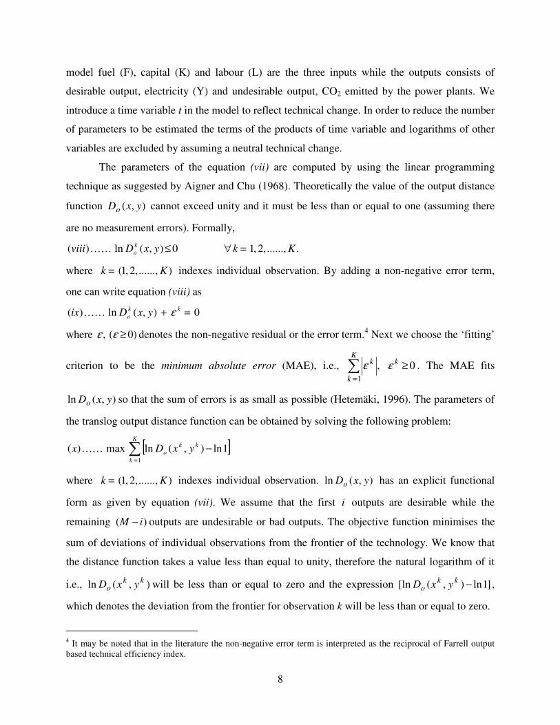
model fuel (F), capital (K) and labour (L) are the three inputs while the outputs consists of

desirable output, electricity (Y) and undesirable output, CO2 emitted by the power plants. We

introduce a time variable t in the model to reflect technical change. In order to reduce the number

of parameters to be estimated the terms of the products of time variable and logarithms of other

variables are excluded by assuming a neutral technical change.

The parameters of the equation (vii) are computed by using the linear programming

technique as suggested by Aigner and Chu (1968). Theoretically the value of the output distance

function ),( yxDo cannot exceed unity and it must be less than or equal to one (assuming there

are no measurement errors). Formally,

.......,,2,10),(ln)( KkyxDviiik

o =∀≤KK

where )......,,2,1( Kk = indexes individual observation. By adding a non-negative error term,

one can write equation (viii) as

0),(ln)( =+ kk

o yxDix εKK

where )0(, ≥εε denotes the non-negative residual or the error term.4 Next we choose the ‘fitting’

criterion to be the minimum absolute error (MAE), i.e., 0,1

≥∑=

kK

k

k εε . The MAE fits

),(ln yxDo so that the sum of errors is as small as possible (Hetemäki, 1996). The parameters of

the translog output distance function can be obtained by solving the following problem:

[ ]∑=

−K

k

kk

o yxDx1

1ln),(lnmax)( KK

where )......,,2,1( Kk = indexes individual observation. ),(ln yxDo has an explicit functional

form as given by equation (vii). We assume that the first i outputs are desirable while the

remaining )( iM − outputs are undesirable or bad outputs. The objective function minimises the

sum of deviations of individual observations from the frontier of the technology. We know that

the distance function takes a value less than equal to unity, therefore the natural logarithm of it

i.e., ),(ln kko yxD will be less than or equal to zero and the expression ]1ln),([ln −kk

o yxD ,

which denotes the deviation from the frontier for observation k will be less than or equal to zero.

4 It may be noted that in the literature the non-negative error term is interpreted as the reciprocal of Farrell output based technical efficiency index.

9

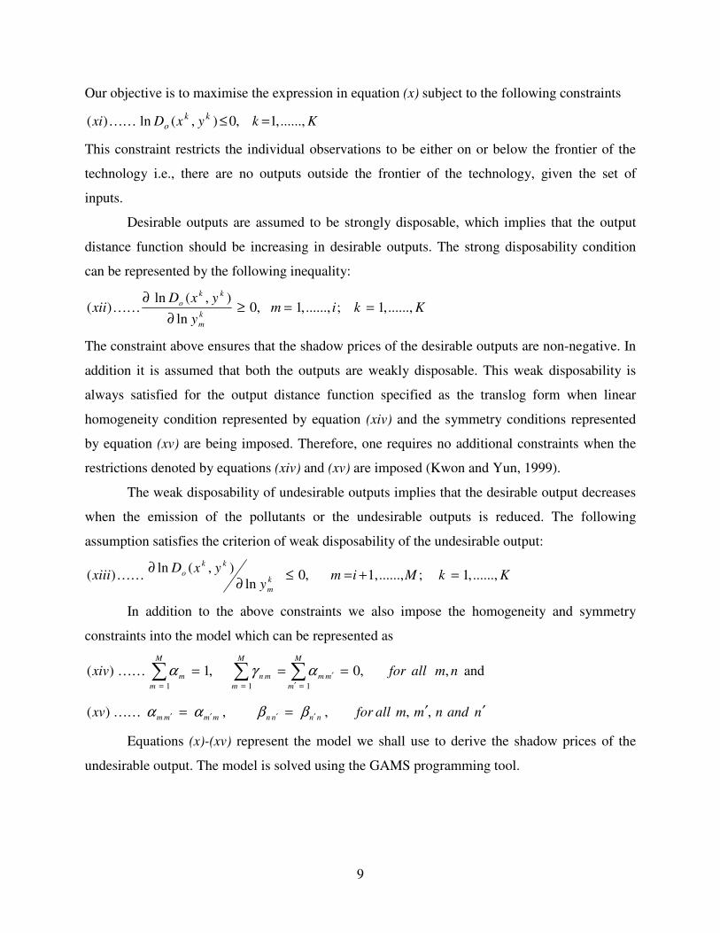
Our objective is to maximise the expression in equation (x) subject to the following constraints

KkyxDxikk

o ......,,1,0),(ln)( =≤KK

This constraint restricts the individual observations to be either on or below the frontier of the

technology i.e., there are no outputs outside the frontier of the technology, given the set of

inputs.

Desirable outputs are assumed to be strongly disposable, which implies that the output

distance function should be increasing in desirable outputs. The strong disposability condition

can be represented by the following inequality:

Kkimy

yxDxii

k

m

kk

o ......,,1;......,,1,0ln

),(ln)( ==≥

∂

∂KK

The constraint above ensures that the shadow prices of the desirable outputs are non-negative. In

addition it is assumed that both the outputs are weakly disposable. This weak disposability is

always satisfied for the output distance function specified as the translog form when linear

homogeneity condition represented by equation (xiv) and the symmetry conditions represented

by equation (xv) are being imposed. Therefore, one requires no additional constraints when the

restrictions denoted by equations (xiv) and (xv) are imposed (Kwon and Yun, 1999).

The weak disposability of undesirable outputs implies that the desirable output decreases

when the emission of the pollutants or the undesirable outputs is reduced. The following

assumption satisfies the criterion of weak disposability of the undesirable output:

KkMimy

yxDxiii k

m

kk

o ......,,1;......,,1,0ln

),(ln)( =+=≤

∂∂

KK

In addition to the above constraints we also impose the homogeneity and symmetry

constraints into the model which can be represented as

nmallforxivM

m

mm

M

m

mn

M

m

m ,,0,1)(111

=== ∑∑∑=′

′

==

αγαKK and

nandnmmallforxv nnnnmmmm′′== ′′′′ ,,,,)( ββααKK

Equations (x)-(xv) represent the model we shall use to derive the shadow prices of the

undesirable output. The model is solved using the GAMS programming tool.

10

4. Data and Estimation Procedure

The empirical analysis is based on primary data collected from the coal fired thermal

plants under the Calcutta Electricity Supply Corporation (CESC), West Bengal Power

Development Corporation Limited (WBPDCL) and Damodar Valley Corporation (DVC) in the

Eastern region of India. These coal fired thermal plants are a part of the Eastern Grid.5 We have

collected detailed data on inputs and outputs for the years 1990-91 to 1999-2000 for all the

thermal plants listed above. However, the data for the Mejia TPS and Budge-Budge TPS were

available for the years 1997-98 to 1999-2000 as these thermal plants were commissioned in the

year 1997 and had started commercial production only from the year 1997-98. A detailed table

listing the various thermal power stations along with the year of commissioning of their

respective units is presented in Table A1 in the appendix. An interesting feature worth

mentioning about our sample of thermal plants is that these plants are of different vintages. On

the one hand we have plants like Bokaro TPS’A’ which was commissioned in the decade of

fifties, there are newer plants like Mejia TPS and Budge-Budge TPS which are still under

construction and only some of their units have started commercial operations on the other.

Moreover, there are also plants that were commissioned in the decades of eighties and nineties.

So we have a whole spectrum of thermal plants in the analysis representing technologies of

different vintages. The primary data pertaining to inputs and outputs were collected from the

WBSEB, DVC and CESC for their respective thermal plants. Only plant level data on inputs,

outputs and prices of one of the desirable output is needed for our analysis.

Inputs: The main inputs needed for generation of electricity by the thermal plants are fuel, capital

and labour. The major fuel input needed by the power plants considered in the present study is

coal. In addition, the coal fired thermal plants also require fuel oil or light diesel oil (LDO), as a

secondary fuel to provide the necessary heat input as and when required to start-up the boiler or

for stabilization of flame at low load. Coal consumption figures are given in metric tonnes while

the fuel oil (or LDO) consumption is recorded in kilolitres. The data pertaining to coal and fuel

oil consumed by the power plants are converted from their respective units to tonnes of oil

equivalent (See Box 1 for conversion factors) and are then aggregated to get the total fuel

consumption figure for the individual plants.

11

Box 1: Conversion Factors

1 Kilolitre of LDO = 0.863 metric tonnes of LDO

1 Metric tonne of LDO = 1.035 tonne of oil equivalent

1 Metric tonne of Coal = 0.67 tonnes of oil equivalent

Source: India, Ministry of Petroleum and Natural Gas (MPNG), (various years), Indian Petroleum and

Natural Gas Statistics, (New Delhi: MPNG, various years). The other important inputs in the generation of electricity are capital and labour. In the

present study we have used the plant capacity in megawatt (MW) as the capital variable

following Kwon and Yun (1999). The data on labour input cover both production and non-

production (white-collar) workers employed in the plant.

Outputs: The output variable consists of both desirable and undesirable outputs. While electricity

generated by the thermal plant is the desirable output and is measured in Megawatt hours (Mwh),

CO2 emission is the bad output. We have used for the desirable output the plant-wise electricity

generation data which was made available by the WBSEB, DVC and CESC for their respective

thermal plants for the period 1990-91 to 1999-2000.

Coal is burnt to generate electricity in the thermal plants. Since in coal carbon is bundled

with ash, carbon, sulfur etc., its burning results in the emission of carbon dioxide, particulate

matters, NOx, etc., in the atmosphere as pollutants. The emission of these pollutants in the

atmosphere can be regarded as the byproduct of electricity generation, and thus is considered as

the undesirable output. The present study considers carbon dioxide as the only undesirable

output. The data relating to the emission of CO2 are not readily available, as most of the thermal

plants in India still do not measure the emissions of CO2. As a result we have used the data on

fuel consumption for generating the data on CO2 emissions. Having obtained the plant wise data

on the consumption of coal and fuel oil or LDO, the emission factors of various fuels given by

IPCC (1995) was used to derive plant wise total CO2 emissions. We also collected data on the

calorific value of coal consumed by the thermal plants in the sample and found that the coal

supplied to these thermal plants is of a higher grade and has a higher calorific value vis-à-vis

those used in most thermal plants in India. In the present study while calculating plant-wise CO2

emissions from burning of coal the calorific values of different grades of coal consumed by the

5 The thermal plants included in the empirical model are Kolaghat Thermal Power Station (KTPS) under the WBPDCL, Bokaro TPS ‘A’, Bokaro TPS ‘B’, Chandrapura TPS, Durgapur TPS, Mejia TPS under the DVC and

12

power plants were incorporated and the CO2 emission factors for coal provided by the IPCC

were adjusted accordingly.6

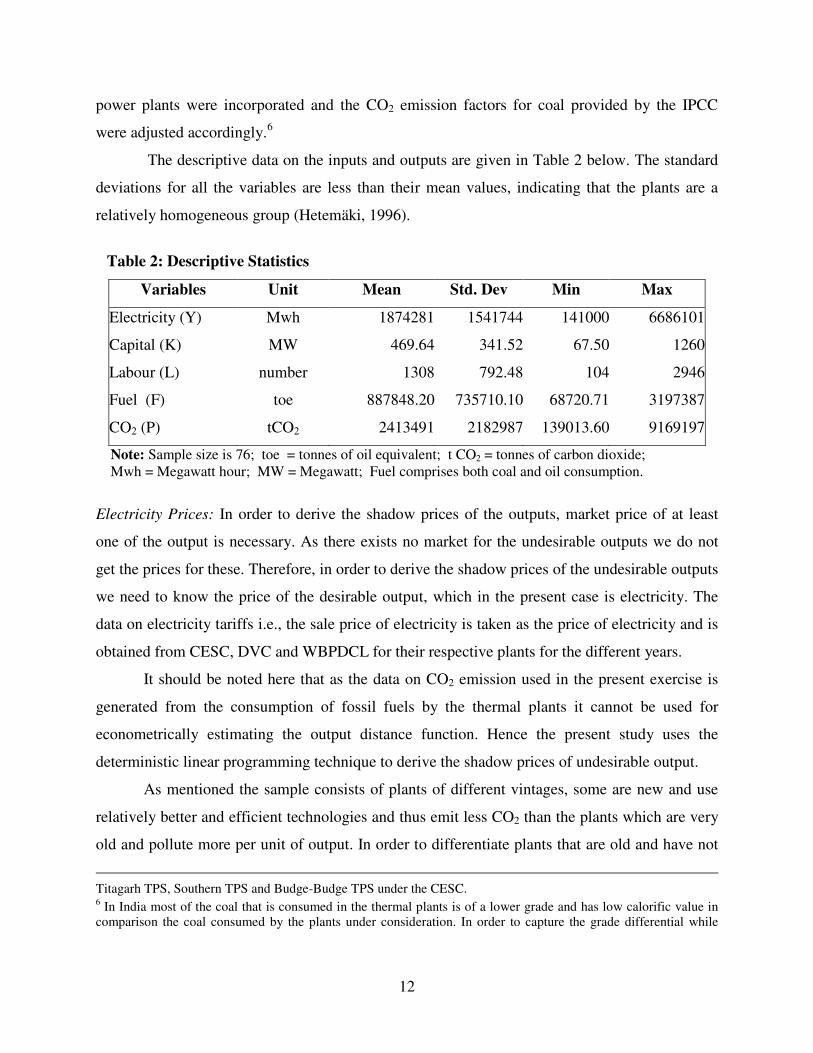
The descriptive data on the inputs and outputs are given in Table 2 below. The standard

deviations for all the variables are less than their mean values, indicating that the plants are a

relatively homogeneous group (Hetemäki, 1996).

Table 2: Descriptive Statistics

Variables Unit Mean Std. Dev Min Max

Electricity (Y) Mwh 1874281 1541744 141000 6686101

Capital (K) MW 469.64 341.52 67.50 1260

Labour (L) number 1308 792.48 104 2946

Fuel (F) toe 887848.20 735710.10 68720.71 3197387

CO2 (P) tCO2 2413491 2182987 139013.60 9169197

Note: Sample size is 76; toe = tonnes of oil equivalent; t CO2 = tonnes of carbon dioxide; Mwh = Megawatt hour; MW = Megawatt; Fuel comprises both coal and oil consumption.

Electricity Prices: In order to derive the shadow prices of the outputs, market price of at least

one of the output is necessary. As there exists no market for the undesirable outputs we do not

get the prices for these. Therefore, in order to derive the shadow prices of the undesirable outputs

we need to know the price of the desirable output, which in the present case is electricity. The

data on electricity tariffs i.e., the sale price of electricity is taken as the price of electricity and is

obtained from CESC, DVC and WBPDCL for their respective plants for the different years.

It should be noted here that as the data on CO2 emission used in the present exercise is

generated from the consumption of fossil fuels by the thermal plants it cannot be used for

econometrically estimating the output distance function. Hence the present study uses the

deterministic linear programming technique to derive the shadow prices of undesirable output.

As mentioned the sample consists of plants of different vintages, some are new and use

relatively better and efficient technologies and thus emit less CO2 than the plants which are very

old and pollute more per unit of output. In order to differentiate plants that are old and have not

Titagarh TPS, Southern TPS and Budge-Budge TPS under the CESC. 6 In India most of the coal that is consumed in the thermal plants is of a lower grade and has low calorific value in comparison the coal consumed by the plants under consideration. In order to capture the grade differential while

13

installed any equipment to control their emissions i.e., the dirty plants, from the plants that use

new technology which is less polluting and plants which have old technology but have installed

equipment or have taken additional measure to restrict emissions and hence pollute less i.e., the

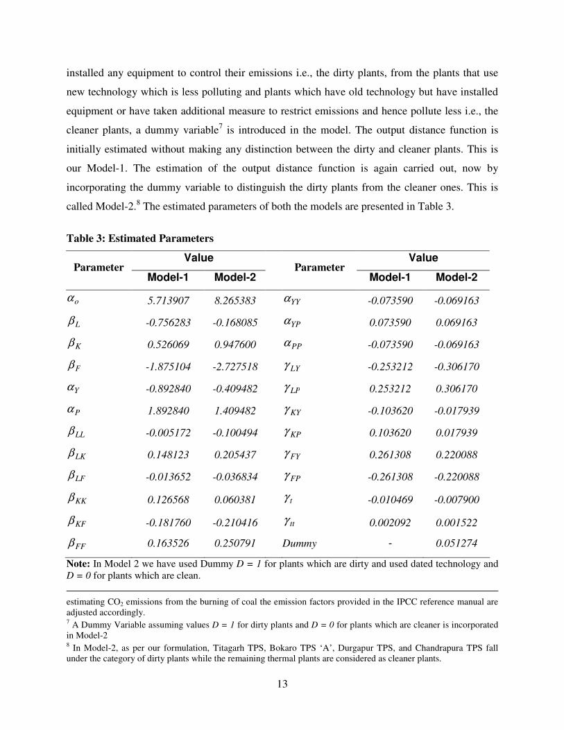
cleaner plants, a dummy variable7 is introduced in the model. The output distance function is

initially estimated without making any distinction between the dirty and cleaner plants. This is

our Model-1. The estimation of the output distance function is again carried out, now by

incorporating the dummy variable to distinguish the dirty plants from the cleaner ones. This is

called Model-2.8 The estimated parameters of both the models are presented in Table 3.

Table 3: Estimated Parameters

Value Value Parameter

Model-1 Model-2 Parameter

Model-1 Model-2

oα 5.713907 8.265383 YYα -0.073590 -0.069163

Lβ -0.756283 -0.168085 YPα 0.073590 0.069163

Kβ 0.526069 0.947600 PPα -0.073590 -0.069163

Fβ -1.875104 -2.727518 LYγ -0.253212 -0.306170

Yα -0.892840 -0.409482 LPγ 0.253212 0.306170

Pα 1.892840 1.409482 KYγ -0.103620 -0.017939

LLβ -0.005172 -0.100494 KPγ 0.103620 0.017939

LKβ 0.148123 0.205437 FYγ 0.261308 0.220088

LFβ -0.013652 -0.036834 FPγ -0.261308 -0.220088

KKβ 0.126568 0.060381 tγ -0.010469 -0.007900

KFβ -0.181760 -0.210416 ttγ 0.002092 0.001522

FFβ 0.163526 0.250791 Dummy - 0.051274

Note: In Model 2 we have used Dummy D = 1 for plants which are dirty and used dated technology and D = 0 for plants which are clean.

estimating CO2 emissions from the burning of coal the emission factors provided in the IPCC reference manual are adjusted accordingly. 7 A Dummy Variable assuming values D = 1 for dirty plants and D = 0 for plants which are cleaner is incorporated in Model-2 8 In Model-2, as per our formulation, Titagarh TPS, Bokaro TPS ‘A’, Durgapur TPS, and Chandrapura TPS fall under the category of dirty plants while the remaining thermal plants are considered as cleaner plants.

14

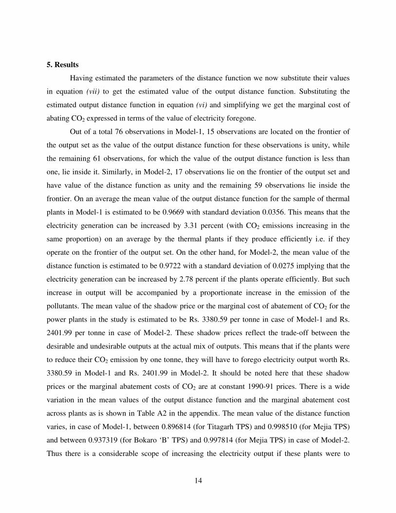
5. Results

Having estimated the parameters of the distance function we now substitute their values

in equation (vii) to get the estimated value of the output distance function. Substituting the

estimated output distance function in equation (vi) and simplifying we get the marginal cost of

abating CO2 expressed in terms of the value of electricity foregone.

Out of a total 76 observations in Model-1, 15 observations are located on the frontier of

the output set as the value of the output distance function for these observations is unity, while

the remaining 61 observations, for which the value of the output distance function is less than

one, lie inside it. Similarly, in Model-2, 17 observations lie on the frontier of the output set and

have value of the distance function as unity and the remaining 59 observations lie inside the

frontier. On an average the mean value of the output distance function for the sample of thermal

plants in Model-1 is estimated to be 0.9669 with standard deviation 0.0356. This means that the

electricity generation can be increased by 3.31 percent (with CO2 emissions increasing in the

same proportion) on an average by the thermal plants if they produce efficiently i.e. if they

operate on the frontier of the output set. On the other hand, for Model-2, the mean value of the

distance function is estimated to be 0.9722 with a standard deviation of 0.0275 implying that the

electricity generation can be increased by 2.78 percent if the plants operate efficiently. But such

increase in output will be accompanied by a proportionate increase in the emission of the

pollutants. The mean value of the shadow price or the marginal cost of abatement of CO2 for the

power plants in the study is estimated to be Rs. 3380.59 per tonne in case of Model-1 and Rs.

2401.99 per tonne in case of Model-2. These shadow prices reflect the trade-off between the

desirable and undesirable outputs at the actual mix of outputs. This means that if the plants were

to reduce their CO2 emission by one tonne, they will have to forego electricity output worth Rs.

3380.59 in Model-1 and Rs. 2401.99 in Model-2. It should be noted here that these shadow

prices or the marginal abatement costs of CO2 are at constant 1990-91 prices. There is a wide

variation in the mean values of the output distance function and the marginal abatement cost

across plants as is shown in Table A2 in the appendix. The mean value of the distance function

varies, in case of Model-1, between 0.896814 (for Titagarh TPS) and 0.998510 (for Mejia TPS)

and between 0.937319 (for Bokaro ‘B’ TPS) and 0.997814 (for Mejia TPS) in case of Model-2.

Thus there is a considerable scope of increasing the electricity output if these plants were to

15

operate efficiently. Similarly, there is a wide variation in the mean value of the output distance

function and the mean value of the marginal abatement costs of CO2 across years as is seen in

Table A3 in the appendix.

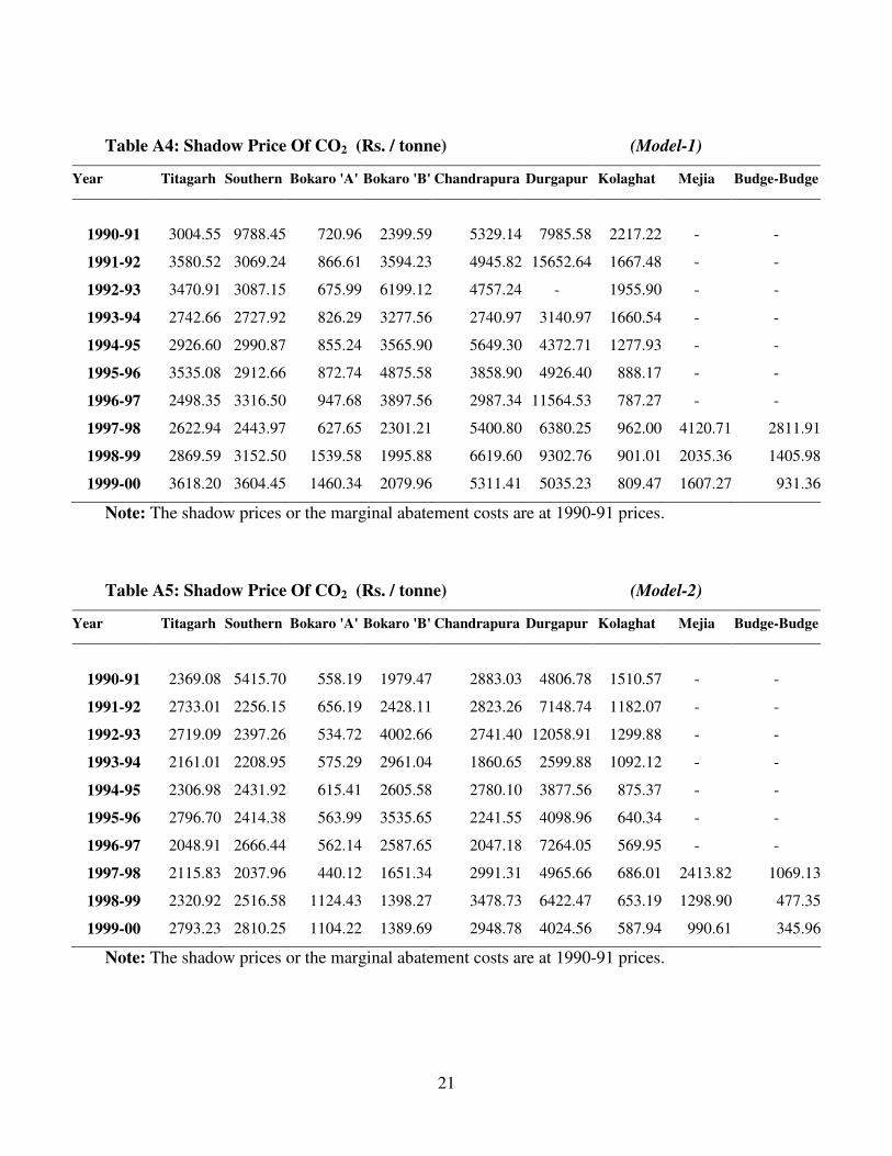
In both the models there is wide variation in the marginal abatement cost across plants.

Even for a particular plant there are variations in the shadow prices across different years (Refer

to Tables A4 and A5 in the Appendix). The wide variation in the marginal abatement costs or the

shadow prices of CO2 can be explained by the variation in the ratio of CO2 emissions to

electricity generation, the different vintages of capital used by the different plants for generation

of power and the different measures adopted for abating or controlling pollution. The variations

in the marginal abatement costs by plant have an important implication in evaluating the cost

effectiveness of the current environmental policies in India. These differences in the marginal

abatement costs across plants are important because of their policy implications. They suggest,

per se, the current pollution control regulations in the country cause an inefficient allocation of

abatement resources across plants and a market oriented system would potentially result in

transfer of such resources across plants and this would lead to cost effectiveness.

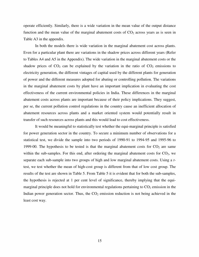
It would be meaningful to statistically test whether the equi-marginal principle is satisfied

for power generation sector in the country. To secure a minimum number of observations for a

statistical test, we divide the sample into two periods of 1990-91 to 1994-95 and 1995-96 to

1999-00. The hypothesis to be tested is that the marginal abatement costs for CO2 are same

within the sub-samples. For this end, after ordering the marginal abatement costs for CO2, we

separate each sub-sample into two groups of high and low marginal abatement costs. Using a t-

test, we test whether the mean of high-cost group is different from that of low cost group. The

results of the test are shown in Table 5. From Table 5 it is evident that for both the sub-samples,

the hypothesis is rejected at 1 per cent level of significance, thereby implying that the equi-

marginal principle does not hold for environmental regulations pertaining to CO2 emission in the

Indian power generation sector. Thus, the CO2 emission reduction is not being achieved in the

least cost way.

16

Table 5: Test results for cost-effectiveness

t-value Period

Model-1 Model-2

1990-91 to 1994-95 4.280 4.017

1995-96 to 1999-00 6.339 7.030

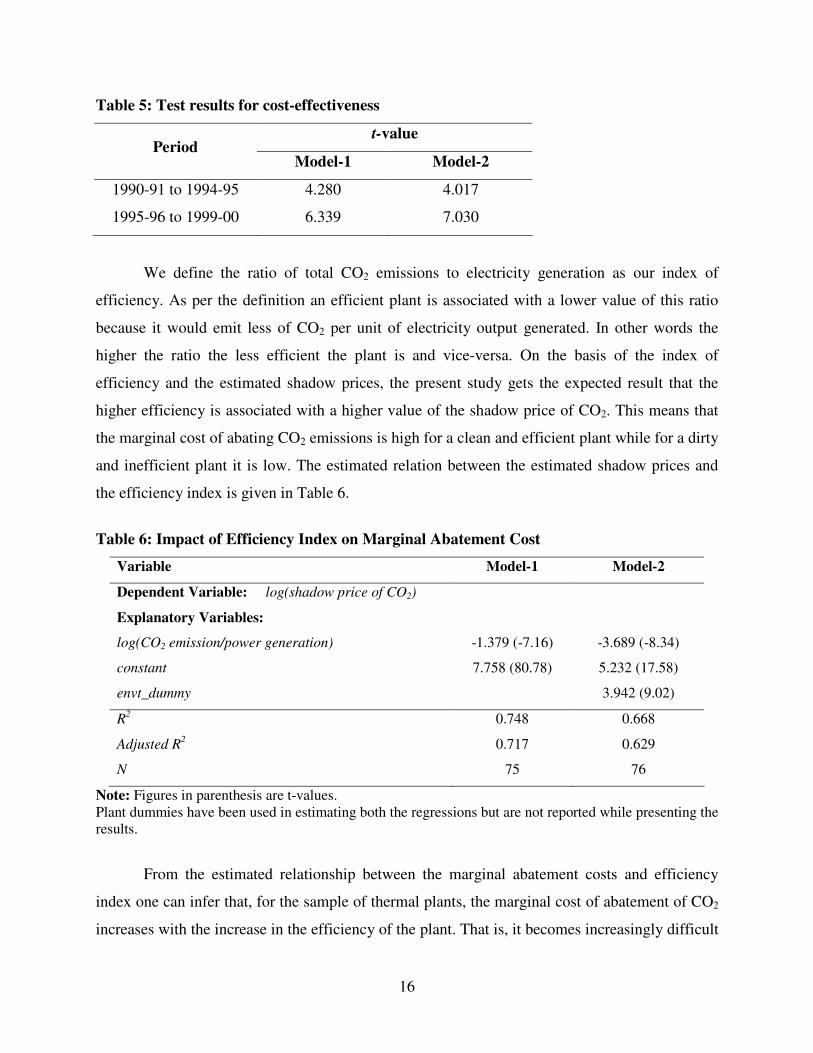
We define the ratio of total CO2 emissions to electricity generation as our index of

efficiency. As per the definition an efficient plant is associated with a lower value of this ratio

because it would emit less of CO2 per unit of electricity output generated. In other words the

higher the ratio the less efficient the plant is and vice-versa. On the basis of the index of

efficiency and the estimated shadow prices, the present study gets the expected result that the

higher efficiency is associated with a higher value of the shadow price of CO2. This means that

the marginal cost of abating CO2 emissions is high for a clean and efficient plant while for a dirty

and inefficient plant it is low. The estimated relation between the estimated shadow prices and

the efficiency index is given in Table 6.

Table 6: Impact of Efficiency Index on Marginal Abatement Cost

Variable Model-1 Model-2

Dependent Variable: log(shadow price of CO2)

Explanatory Variables:

log(CO2 emission/power generation) -1.379 (-7.16) -3.689 (-8.34)

constant 7.758 (80.78) 5.232 (17.58)

envt_dummy 3.942 (9.02)

R2 0.748 0.668

Adjusted R2 0.717 0.629

N 75 76

Note: Figures in parenthesis are t-values. Plant dummies have been used in estimating both the regressions but are not reported while presenting the results.

From the estimated relationship between the marginal abatement costs and efficiency

index one can infer that, for the sample of thermal plants, the marginal cost of abatement of CO2

increases with the increase in the efficiency of the plant. That is, it becomes increasingly difficult

17

or expensive for a plant, which has invested in pollution abating technology or equipment and is

emitting less of CO2 per unit of output to reduce an additional unit of the pollutant vis-à-vis

plants that emit more CO2 per unit of electricity generation. Thus, for a given level of output the

less one pollutes, the higher will be the cost of reducing an additional unit of the pollutant and

vice-versa.

6. Conclusion

There have been a number of studies for India, which have applied the output distance

function approach to calculate the shadow prices of the undesirable outputs. These studies

mainly relate to water pollutants like BOD (biological oxygen demand), COD (chemical oxygen

demand), and SS (suspended solids) (Refer to studies by Murty and S. Kumar 2001, 2002). The

present study is one of the few to use the output distance function technique for the coal fired

thermal plants in India and perhaps the only one to calculate the shadow price of CO2 emissions

for the power sector India. The only other study that uses the output distance technique to

calculate the shadow prices of the pollutants emitted by the power plants in India, is Kumar

(1999) which uses both deterministic and stochastic output distance function technique to derive

the shadow price of (PM10) for the power plants in India. Apart from the studies relating to India,

numerous other studies have also been carried out worldwide to derive the shadow prices of the

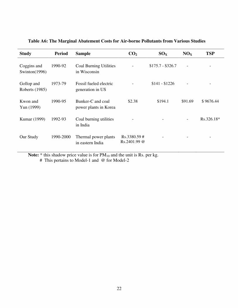
pollutants using the output distance technique. Appendix Table A6 displays the results of some

of the studies that use the output distance function technique to derive the shadow price(s) of

pollutant(s) for the power sector.

The present study uses the output distance function approach and its duality with the

revenue function to calculate the plant specific shadow prices of CO2, for the coal fired thermal

power plants in India. A distinguishing feature of this framework is that it provides a measure of

productive efficiency for each producer. The output distance function technique, since it allows

shadow prices to vary across producers, can reveal a pattern of variation by production

techniques, by other plant characteristics like the age of the plant, volume of pollution etc. This

type of information would be helpful for policy makers in designing or formulating policies to

reduce carbon dioxide emissions.

Economic theory suggests that equalization of the marginal cost of abatement across the

firms would minimise the total cost of abating the pollutants at an aggregate level. The results of

18

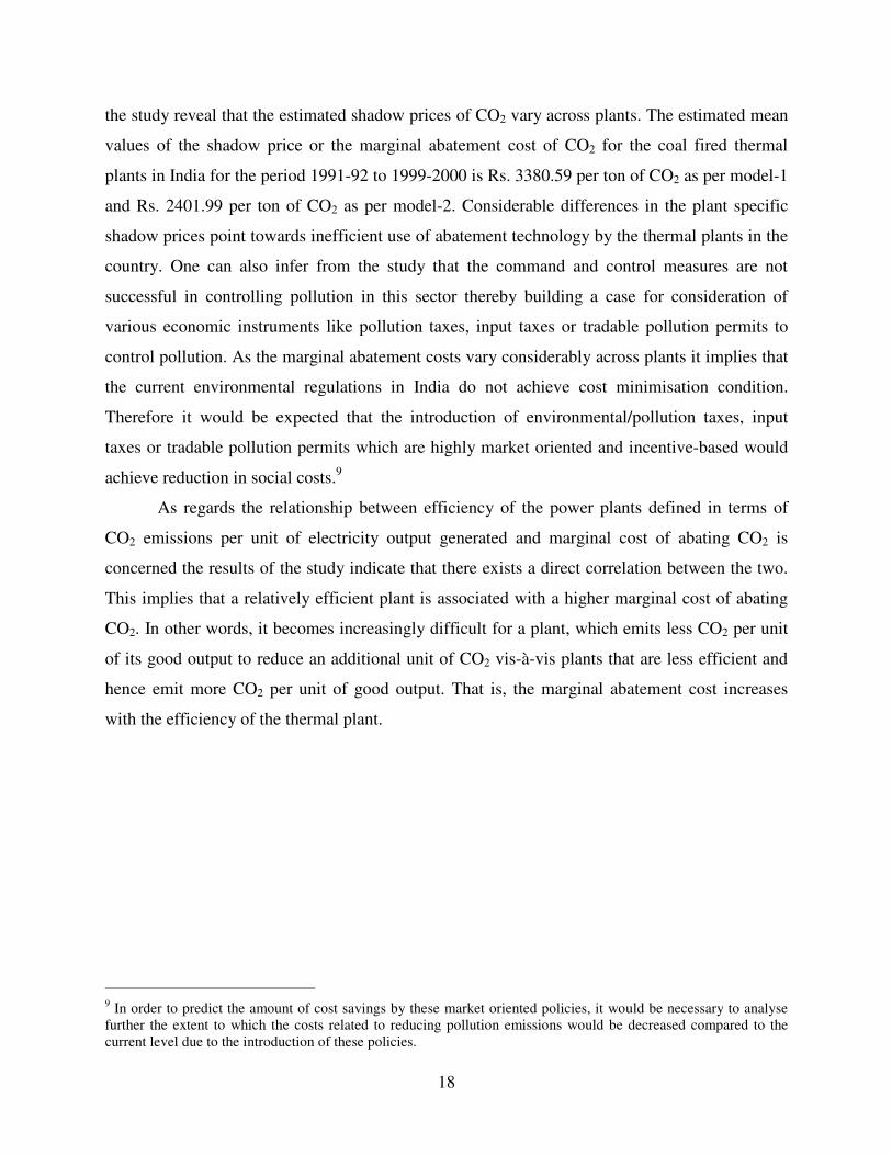
the study reveal that the estimated shadow prices of CO2 vary across plants. The estimated mean

values of the shadow price or the marginal abatement cost of CO2 for the coal fired thermal

plants in India for the period 1991-92 to 1999-2000 is Rs. 3380.59 per ton of CO2 as per model-1

and Rs. 2401.99 per ton of CO2 as per model-2. Considerable differences in the plant specific

shadow prices point towards inefficient use of abatement technology by the thermal plants in the

country. One can also infer from the study that the command and control measures are not

successful in controlling pollution in this sector thereby building a case for consideration of

various economic instruments like pollution taxes, input taxes or tradable pollution permits to

control pollution. As the marginal abatement costs vary considerably across plants it implies that

the current environmental regulations in India do not achieve cost minimisation condition.

Therefore it would be expected that the introduction of environmental/pollution taxes, input

taxes or tradable pollution permits which are highly market oriented and incentive-based would

achieve reduction in social costs.9

As regards the relationship between efficiency of the power plants defined in terms of

CO2 emissions per unit of electricity output generated and marginal cost of abating CO2 is

concerned the results of the study indicate that there exists a direct correlation between the two.

This implies that a relatively efficient plant is associated with a higher marginal cost of abating

CO2. In other words, it becomes increasingly difficult for a plant, which emits less CO2 per unit

of its good output to reduce an additional unit of CO2 vis-à-vis plants that are less efficient and

hence emit more CO2 per unit of good output. That is, the marginal abatement cost increases

with the efficiency of the thermal plant.

9 In order to predict the amount of cost savings by these market oriented policies, it would be necessary to analyse further the extent to which the costs related to reducing pollution emissions would be decreased compared to the current level due to the introduction of these policies.

19

Appendix

Table A1: Details of the Various Thermal Power Stations (TPS)

Thermal Power

Stations

Units Year of

Commissioning

Thermal Power

Stations

Units Year of

Commissioning

Calcutta Electric Supply Corporation Damodar Valley Corporation

Bokaro TPS "A" Unit 1 February 1953 Titagarh TPS Unit 1 1983 Unit 2 August 1953 Unit 2 1983 Unit 3 October 1953 Unit 3 1984 Unit 4 1 April 1960 Unit 4 1985 Bokaro TPS "B" Unit 1 12 March 1987 Southern TPS Unit 1 1990 Unit 2 15 December 1991 Unit 2 1991 Unit 3 1 April 1968 Budge-Budge TPS Unit 1 1997 Chandrapura TPS Unit 1 November 1968 Unit 2 1999 Unit 2 April 1965 Unit 3 1 August 1968 Unit 4 31 March 1975 West Bengal Power Development Corporation Ltd. Unit 5 1 April 1976 Unit 6 1 April 1980 Kolaghat TPS Unit 1 9 September 1990 Unit 2 9 March 1986 Durgapur TPS Unit 1 December 1960 Unit 3 12 October 1984 Unit 2 * February 1961 Unit 4 1 April 1995 Unit 3 * 1 April 1967 Unit 5 14 May 1991 Unit 4 1 December 1982 Unit 6 1 January 1994 Mejia TPS Unit 1 1 December 1997 Unit 2 15 March 1999 Unit 3 28 September 1999

Note: * Decommissioned due to fire since 23 October 1985.

20

Table A2: Mean Values of Output Distance Function and Shadow Prices Across Plants

Model-1 Model-2

Thermal Plants Distance

Function

Shadow Price

(Rs. / tonne)

Distance

Function

Shadow Price

(Rs. / tonne)

Titagarh TPS 0.896814 3086.94 0.966136 2436.48

Southern TPS 0.964838 3709.37 0.965143 2715.56

Bokaro TPS 'A' 0.965746 939.31 0.976638 673.47

Bokaro TPS 'B' 0.977155 3418.66 0.937319 2453.95

Chandrapura TPS 0.984893 4760.05 0.984939 2679.60

Durgapur TPS 0.981496 7595.67 0.988897 5726.76

Kolaghat TPS 0.986287 1312.70 0.982368 909.74

Mejia TPS 0.998510 2587.78 0.997814 1567.78

Budge-Budge TPS 0.972593 1716.42 0.960523 630.81

Overall 0.966916 3380.59 0.972229 2401.99

Note: The values of the shadow price or marginal abatement costs of CO2 abatement are at 1990-91 Prices; TPS = Thermal Power Station.

Table A3: Mean Values of Output Distance Function and Shadow Prices Across Years

Model-1 Model-2

Year Distance

Function

Shadow Price

(Rs. / tonne)

Distance

Function

Shadow Price

(Rs. / tonne)

1990-91 0.961592 4492.213 0.973064 2788.97

1991-92 0.961590 4768.077 0.972118 2746.79

1992-93 0.961934 3357.720 0.973692 3679.13

1993-94 0.967121 2445.274 0.972898 1922.71

1994-95 0.971794 3091.220 0.976806 2213.27

1995-96 0.969427 3124.218 0.971137 2327.37

1996-97 0.959193 3714.176 0.961707 2535.19

1997-98 0.979707 3074.603 0.981455 2041.24

1998-99 0.968473 3313.584 0.971292 2187.87

1999-00 0.964824 2717.520 0.967193 1888.36

Overall 0.966916 3380.59 0.972229 2401.99

Note: The values of the shadow price or marginal abatement costs of CO2 abatement are at 1990-91 prices; The numbers of plants in out study which were seven till 1996-97 increased to nine from the year 1997-98 with the commissioning of two new plants.

21

Table A4: Shadow Price Of CO2 (Rs. / tonne) (Model-1)

Year Titagarh Southern Bokaro 'A' Bokaro 'B' Chandrapura Durgapur Kolaghat Mejia Budge-Budge

1990-91 3004.55 9788.45 720.96 2399.59 5329.14 7985.58 2217.22 - -

1991-92 3580.52 3069.24 866.61 3594.23 4945.82 15652.64 1667.48 - -

1992-93 3470.91 3087.15 675.99 6199.12 4757.24 - 1955.90 - -

1993-94 2742.66 2727.92 826.29 3277.56 2740.97 3140.97 1660.54 - -

1994-95 2926.60 2990.87 855.24 3565.90 5649.30 4372.71 1277.93 - -

1995-96 3535.08 2912.66 872.74 4875.58 3858.90 4926.40 888.17 - -

1996-97 2498.35 3316.50 947.68 3897.56 2987.34 11564.53 787.27 - -

1997-98 2622.94 2443.97 627.65 2301.21 5400.80 6380.25 962.00 4120.71 2811.91

1998-99 2869.59 3152.50 1539.58 1995.88 6619.60 9302.76 901.01 2035.36 1405.98

1999-00 3618.20 3604.45 1460.34 2079.96 5311.41 5035.23 809.47 1607.27 931.36

Note: The shadow prices or the marginal abatement costs are at 1990-91 prices.

Table A5: Shadow Price Of CO2 (Rs. / tonne) (Model-2)

Year Titagarh Southern Bokaro 'A' Bokaro 'B' Chandrapura Durgapur Kolaghat Mejia Budge-Budge

1990-91 2369.08 5415.70 558.19 1979.47 2883.03 4806.78 1510.57 - -

1991-92 2733.01 2256.15 656.19 2428.11 2823.26 7148.74 1182.07 - -

1992-93 2719.09 2397.26 534.72 4002.66 2741.40 12058.91 1299.88 - -

1993-94 2161.01 2208.95 575.29 2961.04 1860.65 2599.88 1092.12 - -

1994-95 2306.98 2431.92 615.41 2605.58 2780.10 3877.56 875.37 - -

1995-96 2796.70 2414.38 563.99 3535.65 2241.55 4098.96 640.34 - -

1996-97 2048.91 2666.44 562.14 2587.65 2047.18 7264.05 569.95 - -

1997-98 2115.83 2037.96 440.12 1651.34 2991.31 4965.66 686.01 2413.82 1069.13

1998-99 2320.92 2516.58 1124.43 1398.27 3478.73 6422.47 653.19 1298.90 477.35

1999-00 2793.23 2810.25 1104.22 1389.69 2948.78 4024.56 587.94 990.61 345.96

Note: The shadow prices or the marginal abatement costs are at 1990-91 prices.

22

Table A6: The Marginal Abatement Costs for Air-borne Pollutants from Various Studies

Study Period Sample CO2 SOX NOX TSP

Coggins and

Swinton(1996)

1990-92 Coal Burning Utilities

in Wisconsin

- $175.7 - $326.7 - -

Gollop and

Roberts (1985)

1973-79 Fossil fueled electric

generation in US

- $141 - $1226 - -

Kwon and

Yun (1999)

1990-95 Bunker-C and coal

power plants in Korea

$2.38 $194.1 $91.69 $ 9676.44

Kumar (1999) 1992-93 Coal burning utilities

in India

- - - Rs.326.18*

Our Study 1990-2000 Thermal power plants

in eastern India

Rs.3380.59 # Rs.2401.99 @

- - -

Note: * this shadow price value is for PM10 and the unit is Rs. per kg. # This pertains to Model-1 and @ for Model-2

23

References:

Government of India (1998), Economic Survey 1997-98, Economic Department, Ministry of Finance, Government of India, New Delhi.

Baumol, W.J. and W. Oates (1988), The Theory of Environmental Policy, Cambridge University Press, Cambridge, United Kingdom.

Titenberg, T.H. (1985), Emissions Trading: An Exercise in Reforming Pollution Policy, Resources For the Future, Washington DC.

Debreu, G. (1951), “The Coefficient of Resource Utilization”, Econometrica, vol. 22, pp. 14-22.

Malmquist, S. (1953), “Index Numbers and Indifference surfaces,” Trabajos de Estatistica, vol. 4, pp. 209-242.

Shephard, Ronald W. (1953), Cost and Production Functions, Princeton University Press, Princeton.

Shephard, Ronald W. (1970), Theory of Cost and Production Functions, Princeton University Press, Princeton.

Färe, Rolf, S. Grosskopf, C.A.K. Lovell, and S. Yaisawarng (1993), “Derivation of Shadow Prices for Undesirable Outputs: A Distance Function Approach,” The Review of

Economics and Statistics, vol. 75, pp. 374-380.

Coggins, J.S., and J.R. Swinton (1996), “The Price of Pollution: A Dual Approach to Valuing SO2 Allowances,” Journal of Environmental Economics and Management, vol. 30, pp. 58-72.

Hetemäki L. (1996), “Essays on the Impact of Pollution Control on a Firm: A Distance Function Approach”, Finnish Forest Research Institute Research Paper 609, Helsinki Research Centre, Helsinki.

Kwon, O.S. and W.C. Yun (1999), “Estimation of the Marginal Abatement Costs of Airborne Pollutants in Korea’s Power Generation Sector,” Energy Economics, vol. 21, pp. 547-560.

Murty, M.N. and S. Kumar (2002), “Measuring the Cost of Environmentally Sustainable Industrial development in India: A Distance Function Approach,” Environment and

Development Economics, vol. 17, No. 3, pp. 467-486.

Färe, Rolf (1988), Fundamentals of Production Theory, Lecture Notes in Economics and Mathematical Systems, Springer Verlag, Berlin.

Färe, Rolf and D. Primont (1995), Multi-Output Production and Duality: Theory and

Applications, Kluwer Academic Publishers, Boston.

Althin, R. (1994), “Shadow Pricing of Labor: A Translog Distance Function Approach,” Department Of Economics, University of Lund Working Paper Series 33/94, Sweden.

Aigner, D.J. and S.F. Chu (1968), “On Estimating the Industry Production Function,” American

Economic Review, vol. 58, pp. 826-839.

Intergovernmental Panel on Climate Change (1995), Greenhouse Gas Inventory Reference

Manual: Guidelines for National Greenhouse Gas Inventories, Vol. 3, IPCC, Geneva.

24

Gollop, F.M. and M.J. Roberts (1985), “Cost-Minimizing Regulation of Sulfur Emissions: Regional Gains in Electric Power”, The Review of Economics and Statistics, vol. 67, pp. 81-90.

Murty, M. N. and S. Kumar (2001), “Environmental and Economic Accounting for Indian Industry”, Institute of Economic Growth Working Paper Series No. E/212/2001, Delhi.

Kumar, S. (1999), “Economic Evaluation of Development Projects: A Case Analysis of Environmental and Health Implications of Thermal Power Projects in India”, Ph.D. Thesis, Jawaharlal Nehru University, New Delhi.

The Energy and Resources Institute (various years), TERI Energy Data Directory and Yearbook

(TEDDY), TERI, New Delhi.

NOTE DI LAVORO DELLA FONDAZIONE ENI ENRICO MATTEI Fondazione Eni Enrico Mattei Working Paper Series

Our Note di Lavoro are available on the Internet at the following addresses: http://www.feem.it/Feem/Pub/Publications/WPapers/default.html

http://www.ssrn.com/link/feem.html http://www.repec.org

http://agecon.lib.umn.edu

NOTE DI LAVORO PUBLISHED IN 2006

SIEV 1.2006 Anna ALBERINI: Determinants and Effects on Property Values of Participation in Voluntary Cleanup Programs: The Case of Colorado

CCMP 2.2006 Valentina BOSETTI, Carlo CARRARO and Marzio GALEOTTI: Stabilisation Targets, Technical Change and the Macroeconomic Costs of Climate Change Control

CCMP 3.2006 Roberto ROSON: Introducing Imperfect Competition in CGE Models: Technical Aspects and Implications KTHC 4.2006 Sergio VERGALLI: The Role of Community in Migration Dynamics

SIEV 5.2006 Fabio GRAZI, Jeroen C.J.M. van den BERGH and Piet RIETVELD: Modeling Spatial Sustainability: Spatial Welfare Economics versus Ecological Footprint

CCMP 6.2006 Olivier DESCHENES and Michael GREENSTONE: The Economic Impacts of Climate Change: Evidence from Agricultural Profits and Random Fluctuations in Weather

PRCG 7.2006 Michele MORETTO and Paola VALBONESE: Firm Regulation and Profit-Sharing: A Real Option Approach SIEV 8.2006 Anna ALBERINI and Aline CHIABAI: Discount Rates in Risk v. Money and Money v. Money Tradeoffs CTN 9.2006 Jon X. EGUIA: United We Vote CTN 10.2006 Shao CHIN SUNG and Dinko DIMITRO: A Taxonomy of Myopic Stability Concepts for Hedonic Games NRM 11.2006 Fabio CERINA (lxxviii): Tourism Specialization and Sustainability: A Long-Run Policy Analysis

NRM 12.2006 Valentina BOSETTI, Mariaester CASSINELLI and Alessandro LANZA (lxxviii): Benchmarking in Tourism Destination, Keeping in Mind the Sustainable Paradigm

CCMP 13.2006 Jens HORBACH: Determinants of Environmental Innovation – New Evidence from German Panel Data SourcesKTHC 14.2006 Fabio SABATINI: Social Capital, Public Spending and the Quality of Economic Development: The Case of ItalyKTHC 15.2006 Fabio SABATINI: The Empirics of Social Capital and Economic Development: A Critical Perspective CSRM 16.2006 Giuseppe DI VITA: Corruption, Exogenous Changes in Incentives and Deterrence

CCMP 17.2006 Rob B. DELLINK and Marjan W. HOFKES: The Timing of National Greenhouse Gas Emission Reductions in the Presence of Other Environmental Policies

IEM 18.2006 Philippe QUIRION: Distributional Impacts of Energy-Efficiency Certificates Vs. Taxes and Standards CTN 19.2006 Somdeb LAHIRI: A Weak Bargaining Set for Contract Choice Problems

CCMP 20.2006 Massimiliano MAZZANTI and Roberto ZOBOLI: Examining the Factors Influencing Environmental Innovations

SIEV 21.2006 Y. Hossein FARZIN and Ken-ICHI AKAO: Non-pecuniary Work Incentive and Labor Supply

CCMP 22.2006 Marzio GALEOTTI, Matteo MANERA and Alessandro LANZA: On the Robustness of Robustness Checks of the Environmental Kuznets Curve

NRM 23.2006 Y. Hossein FARZIN and Ken-ICHI AKAO: When is it Optimal to Exhaust a Resource in a Finite Time?

NRM 24.2006 Y. Hossein FARZIN and Ken-ICHI AKAO: Non-pecuniary Value of Employment and Natural Resource Extinction

SIEV 25.2006 Lucia VERGANO and Paulo A.L.D. NUNES: Analysis and Evaluation of Ecosystem Resilience: An Economic Perspective

SIEV 26.2006 Danny CAMPBELL, W. George HUTCHINSON and Riccardo SCARPA: Using Discrete Choice Experiments toDerive Individual-Specific WTP Estimates for Landscape Improvements under Agri-Environmental SchemesEvidence from the Rural Environment Protection Scheme in Ireland

KTHC 27.2006 Vincent M. OTTO, Timo KUOSMANEN and Ekko C. van IERLAND: Estimating Feedback Effect in Technical Change: A Frontier Approach

CCMP 28.2006 Giovanni BELLA: Uniqueness and Indeterminacy of Equilibria in a Model with Polluting Emissions

IEM 29.2006 Alessandro COLOGNI and Matteo MANERA: The Asymmetric Effects of Oil Shocks on Output Growth: A Markov-Switching Analysis for the G-7 Countries

KTHC 30.2006 Fabio SABATINI: Social Capital and Labour Productivity in Italy ETA 31.2006 Andrea GALLICE (lxxix): Predicting one Shot Play in 2x2 Games Using Beliefs Based on Minimax Regret

IEM 32.2006 Andrea BIGANO and Paul SHEEHAN: Assessing the Risk of Oil Spills in the Mediterranean: the Case of the Route from the Black Sea to Italy

NRM 33.2006 Rinaldo BRAU and Davide CAO (lxxviii): Uncovering the Macrostructure of Tourists’ Preferences. A Choice Experiment Analysis of Tourism Demand to Sardinia

CTN 34.2006 Parkash CHANDER and Henry TULKENS: Cooperation, Stability and Self-Enforcement in International Environmental Agreements: A Conceptual Discussion

IEM 35.2006 Valeria COSTANTINI and Salvatore MONNI: Environment, Human Development and Economic Growth ETA 36.2006 Ariel RUBINSTEIN (lxxix): Instinctive and Cognitive Reasoning: A Study of Response Times

ETA 37.2006 Maria SALGADeO (lxxix): Choosing to Have Less Choice

ETA 38.2006 Justina A.V. FISCHER and Benno TORGLER: Does Envy Destroy Social Fundamentals? The Impact of Relative Income Position on Social Capital

ETA 39.2006 Benno TORGLER, Sascha L. SCHMIDT and Bruno S. FREY: Relative Income Position and Performance: An Empirical Panel Analysis

CCMP 40.2006 Alberto GAGO, Xavier LABANDEIRA, Fidel PICOS And Miguel RODRÍGUEZ: Taxing Tourism In Spain: Results and Recommendations

IEM 41.2006 Karl van BIERVLIET, Dirk Le ROY and Paulo A.L.D. NUNES: An Accidental Oil Spill Along the Belgian Coast: Results from a CV Study

CCMP 42.2006 Rolf GOLOMBEK and Michael HOEL: Endogenous Technology and Tradable Emission Quotas

KTHC 43.2006 Giulio CAINELLI and Donato IACOBUCCI: The Role of Agglomeration and Technology in Shaping Firm Strategy and Organization

CCMP 44.2006 Alvaro CALZADILLA, Francesco PAULI and Roberto ROSON: Climate Change and Extreme Events: An Assessment of Economic Implications

SIEV 45.2006 M.E. KRAGT, P.C. ROEBELING and A. RUIJS: Effects of Great Barrier Reef Degradation on Recreational Demand: A Contingent Behaviour Approach

NRM 46.2006 C. GIUPPONI, R. CAMERA, A. FASSIO, A. LASUT, J. MYSIAK and A. SGOBBI: Network Analysis, CreativeSystem Modelling and DecisionSupport: The NetSyMoD Approach

KTHC 47.2006 Walter F. LALICH (lxxx): Measurement and Spatial Effects of the Immigrant Created Cultural Diversity in Sydney

KTHC 48.2006 Elena PASPALANOVA (lxxx): Cultural Diversity Determining the Memory of a Controversial Social Event

KTHC 49.2006 Ugo GASPARINO, Barbara DEL CORPO and Dino PINELLI (lxxx): Perceived Diversity of Complex Environmental Systems: Multidimensional Measurement and Synthetic Indicators

KTHC 50.2006 Aleksandra HAUKE (lxxx): Impact of Cultural Differences on Knowledge Transfer in British, Hungarian and Polish Enterprises

KTHC 51.2006 Katherine MARQUAND FORSYTH and Vanja M. K. STENIUS (lxxx): The Challenges of Data Comparison and Varied European Concepts of Diversity

KTHC 52.2006 Gianmarco I.P. OTTAVIANO and Giovanni PERI (lxxx): Rethinking the Gains from Immigration: Theory and Evidence from the U.S.

KTHC 53.2006 Monica BARNI (lxxx): From Statistical to Geolinguistic Data: Mapping and Measuring Linguistic Diversity KTHC 54.2006 Lucia TAJOLI and Lucia DE BENEDICTIS (lxxx): Economic Integration and Similarity in Trade Structures

KTHC 55.2006 Suzanna CHAN (lxxx): “God’s Little Acre” and “Belfast Chinatown”: Diversity and Ethnic Place Identity in Belfast

KTHC 56.2006 Diana PETKOVA (lxxx): Cultural Diversity in People’s Attitudes and Perceptions

KTHC 57.2006 John J. BETANCUR (lxxx): From Outsiders to On-Paper Equals to Cultural Curiosities? The Trajectory of Diversity in the USA

KTHC 58.2006 Kiflemariam HAMDE (lxxx): Cultural Diversity A Glimpse Over the Current Debate in Sweden KTHC 59.2006 Emilio GREGORI (lxxx): Indicators of Migrants’ Socio-Professional Integration

KTHC 60.2006 Christa-Maria LERM HAYES (lxxx): Unity in Diversity Through Art? Joseph Beuys’ Models of Cultural Dialogue

KTHC 61.2006 Sara VERTOMMEN and Albert MARTENS (lxxx): Ethnic Minorities Rewarded: Ethnostratification on the Wage Market in Belgium

KTHC 62.2006 Nicola GENOVESE and Maria Grazia LA SPADA (lxxx): Diversity and Pluralism: An Economist's View

KTHC 63.2006 Carla BAGNA (lxxx): Italian Schools and New Linguistic Minorities: Nationality Vs. Plurilingualism. Which Ways and Methodologies for Mapping these Contexts?

KTHC 64.2006 Vedran OMANOVIĆ (lxxx): Understanding “Diversity in Organizations” Paradigmatically and Methodologically

KTHC 65.2006 Mila PASPALANOVA (lxxx): Identifying and Assessing the Development of Populations of Undocumented Migrants: The Case of Undocumented Poles and Bulgarians in Brussels

KTHC 66.2006 Roberto ALZETTA (lxxx): Diversities in Diversity: Exploring Moroccan Migrants’ Livelihood in Genoa

KTHC 67.2006 Monika SEDENKOVA and Jiri HORAK (lxxx): Multivariate and Multicriteria Evaluation of Labour Market Situation

KTHC 68.2006 Dirk JACOBS and Andrea REA (lxxx): Construction and Import of Ethnic Categorisations: “Allochthones” in The Netherlands and Belgium

KTHC 69.2006 Eric M. USLANER (lxxx): Does Diversity Drive Down Trust?

KTHC 70.2006 Paula MOTA SANTOS and João BORGES DE SOUSA (lxxx): Visibility & Invisibility of Communities in Urban Systems

ETA 71.2006 Rinaldo BRAU and Matteo LIPPI BRUNI: Eliciting the Demand for Long Term Care Coverage: A Discrete Choice Modelling Analysis

CTN 72.2006 Dinko DIMITROV and Claus-JOCHEN HAAKE: Coalition Formation in Simple Games: The Semistrict Core

CTN 73.2006 Ottorino CHILLEM, Benedetto GUI and Lorenzo ROCCO: On The Economic Value of Repeated Interactions Under Adverse Selection

CTN 74.2006 Sylvain BEAL and Nicolas QUÉROU: Bounded Rationality and Repeated Network Formation CTN 75.2006 Sophie BADE, Guillaume HAERINGER and Ludovic RENOU: Bilateral Commitment CTN 76.2006 Andranik TANGIAN: Evaluation of Parties and Coalitions After Parliamentary Elections

CTN 77.2006 Rudolf BERGHAMMER, Agnieszka RUSINOWSKA and Harrie de SWART: Applications of Relations and Graphs to Coalition Formation

CTN 78.2006 Paolo PIN: Eight Degrees of Separation CTN 79.2006 Roland AMANN and Thomas GALL: How (not) to Choose Peers in Studying Groups

CTN 80.2006 Maria MONTERO: Inequity Aversion May Increase Inequity CCMP 81.2006 Vincent M. OTTO, Andreas LÖSCHEL and John REILLY: Directed Technical Change and Climate Policy

CSRM 82.2006 Nicoletta FERRO: Riding the Waves of Reforms in Corporate Law, an Overview of Recent Improvements in Italian Corporate Codes of Conduct

CTN 83.2006 Siddhartha BANDYOPADHYAY and Mandar OAK: Coalition Governments in a Model of Parliamentary Democracy

PRCG 84.2006 Raphaël SOUBEYRAN: Valence Advantages and Public Goods Consumption: Does a Disadvantaged Candidate Choose an Extremist Position?

CCMP 85.2006 Eduardo L. GIMÉNEZ and Miguel RODRÍGUEZ: Pigou’s Dividend versus Ramsey’s Dividend in the Double Dividend Literature

CCMP 86.2006 Andrea BIGANO, Jacqueline M. HAMILTON and Richard S.J. TOL: The Impact of Climate Change on Domestic and International Tourism: A Simulation Study

KTHC 87.2006 Fabio SABATINI: Educational Qualification, Work Status and Entrepreneurship in Italy an Exploratory Analysis

CCMP 88.2006 Richard S.J. TOL: The Polluter Pays Principle and Cost-Benefit Analysis of Climate Change: An Application of Fund

CCMP 89.2006 Philippe TULKENS and Henry TULKENS: The White House and The Kyoto Protocol: Double Standards on Uncertainties and Their Consequences

SIEV 90.2006 Andrea M. LEITER and Gerald J. PRUCKNER: Proportionality of Willingness to Pay to Small Risk Changes – The Impact of Attitudinal Factors in Scope Tests

PRCG 91.2006 Raphäel SOUBEYRAN: When Inertia Generates Political Cycles CCMP 92.2006 Alireza NAGHAVI: Can R&D-Inducing Green Tariffs Replace International Environmental Regulations?

CCMP 93.2006 Xavier PAUTREL: Reconsidering The Impact of Environment on Long-Run Growth When Pollution Influences Health and Agents Have Finite-Lifetime

CCMP 94.2006 Corrado Di MARIA and Edwin van der WERF: Carbon Leakage Revisited: Unilateral Climate Policy with Directed Technical Change

CCMP 95.2006 Paulo A.L.D. NUNES and Chiara M. TRAVISI: Comparing Tax and Tax Reallocations Payments in Financing Rail Noise Abatement Programs: Results from a CE valuation study in Italy

CCMP 96.2006 Timo KUOSMANEN and Mika KORTELAINEN: Valuing Environmental Factors in Cost-Benefit Analysis Using Data Envelopment Analysis

KTHC 97.2006 Dermot LEAHY and Alireza NAGHAVI: Intellectual Property Rights and Entry into a Foreign Market: FDI vs. Joint Ventures

CCMP 98.2006 Inmaculada MARTÍNEZ-ZARZOSO, Aurelia BENGOCHEA-MORANCHO and Rafael MORALES LAGE: The Impact of Population on CO2 Emissions: Evidence from European Countries

PRCG 99.2006 Alberto CAVALIERE and Simona SCABROSETTI: Privatization and Efficiency: From Principals and Agents to Political Economy

NRM 100.2006 Khaled ABU-ZEID and Sameh AFIFI: Multi-Sectoral Uses of Water & Approaches to DSS in Water Management in the NOSTRUM Partner Countries of the Mediterranean

NRM 101.2006 Carlo GIUPPONI, Jaroslav MYSIAK and Jacopo CRIMI: Participatory Approach in Decision Making Processes for Water Resources Management in the Mediterranean Basin

CCMP 102.2006 Kerstin RONNEBERGER, Maria BERRITTELLA, Francesco BOSELLO and Richard S.J. TOL: Klum@Gtap: Introducing Biophysical Aspects of Land-Use Decisions Into a General Equilibrium Model A Coupling Experiment

KTHC 103.2006 Avner BEN-NER, Brian P. McCALL, Massoud STEPHANE, and Hua WANG: Identity and Self-Other Differentiation in Work and Giving Behaviors: Experimental Evidence

SIEV 104.2006 Aline CHIABAI and Paulo A.L.D. NUNES: Economic Valuation of Oceanographic Forecasting Services: A Cost-Benefit Exercise

NRM 105.2006 Paola MINOIA and Anna BRUSAROSCO: Water Infrastructures Facing Sustainable Development Challenges: Integrated Evaluation of Impacts of Dams on Regional Development in Morocco

PRCG 106.2006 Carmine GUERRIERO: Endogenous Price Mechanisms, Capture and Accountability Rules: Theory and Evidence

CCMP 107.2006 Richard S.J. TOL, Stephen W. PACALA and Robert SOCOLOW: Understanding Long-Term Energy Use and Carbon Dioxide Emissions in the Usa

NRM 108.2006 Carles MANERA and Jaume GARAU TABERNER: The Recent Evolution and Impact of Tourism in theMediterranean: The Case of Island Regions, 1990-2002

PRCG 109.2006 Carmine GUERRIERO: Dependent Controllers and Regulation Policies: Theory and Evidence KTHC 110.2006 John FOOT (lxxx): Mapping Diversity in Milan. Historical Approaches to Urban Immigration KTHC 111.2006 Donatella CALABI: Foreigners and the City: An Historiographical Exploration for the Early Modern Period

IEM 112.2006 Andrea BIGANO, Francesco BOSELLO and Giuseppe MARANO: Energy Demand and Temperature: A Dynamic Panel Analysis

SIEV 113.2006 Anna ALBERINI, Stefania TONIN, Margherita TURVANI and Aline CHIABAI: Paying for Permanence: Public Preferences for Contaminated Site Cleanup

CCMP 114.2006 Vivekananda MUKHERJEE and Dirk T.G. RÜBBELKE: Global Climate Change, Technology Transfer and Trade with Complete Specialization

NRM 115.2006 Clive LIPCHIN: A Future for the Dead Sea Basin: Water Culture among Israelis, Palestinians and Jordanians

CCMP 116.2006 Barbara BUCHNER, Carlo CARRARO and A. Denny ELLERMAN: The Allocation of European Union Allowances: Lessons, Unifying Themes and General Principles

CCMP 117.2006 Richard S.J. TOL: Carbon Dioxide Emission Scenarios for the Usa

NRM 118.2006 Isabel CORTÉS-JIMÉNEZ and Manuela PULINA: A further step into the ELGH and TLGH for Spain and Italy

SIEV 119.2006 Beat HINTERMANN, Anna ALBERINI and Anil MARKANDYA: Estimating the Value of Safety with Labor Market Data: Are the Results Trustworthy?

SIEV 120.2006 Elena STRUKOVA, Alexander GOLUB and Anil MARKANDYA: Air Pollution Costs in Ukraine

CCMP 121.2006 Massimiliano MAZZANTI, Antonio MUSOLESI and Roberto ZOBOLI: A Bayesian Approach to the Estimation of Environmental Kuznets Curves for CO2 Emissions

ETA 122.2006 Jean-Marie GRETHER, Nicole A. MATHYS, and Jaime DE MELO: Unraveling the World-Wide Pollution Haven Effect

KTHC 123.2006 Sergio VERGALLI: Entry and Exit Strategies in Migration Dynamics

PRCG 124.2006 Bernardo BORTOLOTTI and Valentina MILELLA: Privatization in Western Europe Stylized Facts, Outcomesand Open Issues

SIEV 125.2006 Pietro CARATTI, Ludovico FERRAGUTO and Chiara RIBOLDI: Sustainable Development Data Availability on the Internet

SIEV 126.2006 S. SILVESTRI, M PELLIZZATO and V. BOATTO: Fishing Across the Centuries: What Prospects for the Venice Lagoon?

CTN 127.2006 Alison WATTS: Formation of Segregated and Integrated Groups

SIEV 128.2006 Danny CAMPBELL, W. George HUTCHINSON and Riccardo SCARPA: Lexicographic Preferences in Discrete Choice Experiments: Consequences on Individual-Specific Willingness to Pay Estimates

CCMP 129.2006 Giovanni BELLA: Transitional Dynamics Towards Sustainability: Reconsidering the EKC Hypothesis

IEM 130.2006 Elisa SCARPA and Matteo MANERA: Pricing and Hedging Illiquid Energy Derivatives: an Application to the JCC Index

PRCG 131.2006 Andrea BELTRATTI and Bernardo BORTOLOTTI: The Nontradable Share Reform in the Chinese Stock Market

IEM 132.2006 Alberto LONGO, Anil MARKANDYA and Marta PETRUCCI: The Internalization of Externalities in The Production of Electricity: Willingness to Pay for the Attributes of a Policy for Renewable Energy

ETA 133.2006 Brighita BERCEA and Sonia OREFFICE: Quality of Available Mates, Education and Intra-Household Bargaining Power

KTHC 134.2006 Antonia R. GURRIERI and Luca PETRUZZELLIS: Local Networks to Compete in the Global Era. The Italian SMEs Experience

CCMP 135.2006 Andrea BIGANO, Francesco BOSELLO, Roberto ROSON and Richard S.J. TOL: Economy-Wide Estimates of the Implications of Climate Change: A Joint Analysis for Sea Level Rise and Tourism

CCMP 136.2006 Richard S.J. TOL: Why Worry About Climate Change? A Research Agenda

SIEV 137.2006 Anna ALBERINI, Alberto LONGO and Patrizia RIGANTI: Using Surveys to Compare the Public’s and Decisionmakers’ Preferences for Urban Regeneration: The Venice Arsenale

ETA 138.2006 Y. Hossein FARZIN and Ken-Ichi AKAO: Environmental Quality in a Differentiated Duopoly

CCMP 139.2006 Denny ELLERMAN and Barbara BUCHNER: Over-Allocation or Abatement?A Preliminary Analysis of the Eu Ets Based on the 2005 Emissions Data

CCMP 140.2006 Horaţiu A. RUS (lxxxi): Renewable Resources, Pollution and Trade in a Small Open Economy

CCMP 141.2006 Enrica DE CIAN (lxxxi): International Technology Spillovers in Climate-Economy Models: Two Possible Approaches

CCMP 142.2006 Tao WANG (lxxxi): Cost Effectiveness in River Management: Evaluation of Integrated River Policy System in Tidal Ouse

CCMP 143.2006 Gregory F. NEMET (lxxxi): How well does Learning-by-doing Explain Cost Reductions in a Carbon-free Energy Technology?

CCMP 144.2006 Anne BRIAND (lxxxi): Marginal Cost Versus Average Cost Pricing with Climatic Shocks in Senegal: ADynamic Computable General Equilibrium Model Applied to Water

CCMP 145.2006 Thomas ARONSSON, Kenneth BACKLUND and Linda SAHLÉN (lxxxi): Technology Transfers and the Clean Development Mechanism in a North-South General Equilibrium Model

IEM 146.2006 Theocharis N. GRIGORIADIS and Benno TORGLER: Energy Regulation, Roll Call Votes and Regional Resources:Evidence from Russia

CCMP 147.2006 Manish GUPTA: Costs of Reducing Greenhouse Gas Emissions: A Case Study of India’s Power Generation Sector

(lxxviii) This paper was presented at the Second International Conference on "Tourism and Sustainable Economic Development - Macro and Micro Economic Issues" jointly organised by CRENoS (Università di Cagliari and Sassari, Italy) and Fondazione Eni Enrico Mattei, Italy, and supported by the World Bank, Chia, Italy, 16-17 September 2005. (lxxix) This paper was presented at the International Workshop on "Economic Theory and Experimental Economics" jointly organised by SET (Center for advanced Studies in Economic Theory, University of Milano-Bicocca) and Fondazione Eni Enrico Mattei, Italy, Milan, 20-23 November 2005. The Workshop was co-sponsored by CISEPS (Center for Interdisciplinary Studies in Economics and Social Sciences, University of Milan-Bicocca). (lxxx) This paper was presented at the First EURODIV Conference “Understanding diversity: Mapping and measuring”, held in Milan on 26-27 January 2006 and supported by the Marie Curie Series of Conferences “Cultural Diversity in Europe: a Series of Conferences. (lxxxi) This paper was presented at the EAERE-FEEM-VIU Summer School on "Computable General Equilibrium Modeling in Environmental and Resource Economics", held in Venice from June 25th to July 1st, 2006 and supported by the Marie Curie Series of Conferences "European Summer School in Resource and Environmental Economics".

2006 SERIES

CCMP Climate Change Modelling and Policy (Editor: Marzio Galeotti )

SIEV Sustainability Indicators and Environmental Valuation (Editor: Anil Markandya)

NRM Natural Resources Management (Editor: Carlo Giupponi)

KTHC Knowledge, Technology, Human Capital (Editor: Gianmarco Ottaviano)

IEM International Energy Markets (Editor: Matteo Manera)

CSRM Corporate Social Responsibility and Sustainable Management (Editor: Giulio Sapelli)

PRCG Privatisation Regulation Corporate Governance (Editor: Bernardo Bortolotti)

ETA Economic Theory and Applications (Editor: Carlo Carraro)

CTN Coalition Theory Network