Cost Avoidance Analysis of Military Aircraft Components ...
76
University of South Carolina Scholar Commons eses and Dissertations 12-15-2014 Cost Avoidance Analysis of Military Aircraſt Components Utilizing Condition-Based Maintenance Practices Erin Ballentine University of South Carolina - Columbia Follow this and additional works at: hps://scholarcommons.sc.edu/etd Part of the Mechanical Engineering Commons is Open Access esis is brought to you by Scholar Commons. It has been accepted for inclusion in eses and Dissertations by an authorized administrator of Scholar Commons. For more information, please contact [email protected]. Recommended Citation Ballentine, E.(2014). Cost Avoidance Analysis of Military Aircraſt Components Utilizing Condition-Based Maintenance Practices. (Master's thesis). Retrieved from hps://scholarcommons.sc.edu/etd/2932
Transcript of Cost Avoidance Analysis of Military Aircraft Components ...

University of South CarolinaScholar Commons
Theses and Dissertations
12-15-2014
Cost Avoidance Analysis of Military AircraftComponents Utilizing Condition-BasedMaintenance PracticesErin BallentineUniversity of South Carolina - Columbia
Follow this and additional works at: https://scholarcommons.sc.edu/etd
Part of the Mechanical Engineering Commons
This Open Access Thesis is brought to you by Scholar Commons. It has been accepted for inclusion in Theses and Dissertations by an authorizedadministrator of Scholar Commons. For more information, please contact [email protected].
Recommended CitationBallentine, E.(2014). Cost Avoidance Analysis of Military Aircraft Components Utilizing Condition-Based Maintenance Practices. (Master'sthesis). Retrieved from https://scholarcommons.sc.edu/etd/2932

COST AVOIDANCE ANALYSIS OF MILITARY AIRCRAFT COMPONENTS
UTILIZING CONDITION-BASED MAINTENANCE PRACTICES
by
Erin Ballentine
Bachelor of Science
University of South Carolina, 2012
Submitted in Partial Fulfillment of the Requirements
For the Degree of Master of Science in
Mechanical Engineering
College of Engineering and Computing
University of South Carolina
2014
Accepted by:
Abdel Bayoumi, Director of Thesis
Richard Robinson, Reader
Lacy Ford, Vice Provost and Dean of Graduate Studies

ii
© Copyright by Erin Ballentine, 2014 All Rights Reserved.

iii
ACKNOWLEDGEMENTS
I would first like to thank my advisor, Dr. Abdel E. Bayoumi, for making me a
part of the CBM team. Without his advice to push myself into unfamiliar areas, I would
not have realized my potential in engineering cost analysis. I would like to thank my
friends and family for their encouragement, guidance, and support throughout my
graduate school experience. I also want to thank the CBM team, particularly Travis
Edwards and Thomas Hartmann, for their contributions to my efforts.
I would like to thank Mr. Lem Grant and retired MG Les Eisner for their constant
support and promotion of the USC CBM program and its goals. Also, for their direct
contributions to my research: CW5 Donald L. Washabaugh (PEOAVN); Dr. Jerry
Higman (Apache PM); Michele K. Platt (AVNIK, in support of Apache PM); Stanley H.
Graves (Camber Corporation in support of AED Aeromechanics); Michael McNulty
(Boeing); Tom Thompson (AED); Jim Hunt (Avion Solutions); CSM Woody Sullivan,
CW2 Adam D. Miracle, SSG Roosevelt Robinson, and SGT Frank Shrev from
SCARNG; and Dr. Richard Robinson, Jr. (Darla Moore School of Business). Lastly, I
would like to thank everyone else who has helped and supported me along the way.

iv
ABSTRACT
This research involves two major case studies. Both look at the current
maintenance practices done by the United States Army and propose a solution for
improvement utilizing condition-based maintenance (CBM) practices. Each study details
a cost avoidance that can be earned by implementing the solutions and the resulting
benefits that can be experienced.
Case Study I is a return on investment (ROI) that analyzes the benefits of the
implementation of elastomeric wedges as vibration control on the Apache (AH-64D)
aircraft. Analysis of the material and operational costs shows that the use of self-adhering
elastomeric trailing edge wedges on the Apache helicopter in main rotor blade tracking
operations will significantly reduce the number of blades damaged by tab bending that
must be repaired at the depot level. Wedge implementation will also allow for a decrease
in the number of test flights and maintenance man hours associated with those flights.
Additionally, the wedges will lower aircraft vibration levels. A 10-year ROI is calculated
for projected peacetime flying hours and for the current flying rate. Dollar values and
flight hour optempo (operating tempo) have been removed and replaced with percentages
or pseudonyms to comply with the operations security process.
Case Study II examines the maintenance practices regarding the GE T700, T701,
T701C, and T701D turboshaft engine. According to the Aviation and Missile
Command’s (AMCOM) integrated priority list, the turboshaft engine is the number one

v
cost burden to the Army with Army Working Capital Fund (AWCF) salesa exceeding
$260M for FY12 and projected salesb over $200M for FY13. Analysis of
Remediation/Reliability Improvement through Failure Identification and Reporting
(RIMFIRE) data on engines determined to be field repairable by depot shows return of
engine modules in lieu of the entire engine yields a significant cost avoidance. Returning
modules instead of engines would reduce the number of field repairable engines sent to
depot by almost 50%. Additional ways to reduce the number of field repairable engines
are discussed and their benefits are included. Dollar values and component demand data
have been removed and replaced with percentages or pseudonyms to comply with the
operations security process.
a Total AWCF Sales (last 12 months) is defined as “Dollar value of the AWCF sales for the last 12 months
calculated by multiplying the AMDF price times the number of independent demands”. The AMDF Price
definition states “Also known as the standard price, it includes the latest acquisition cost plus the authorized
cost recovery rate (surcharge)”. Independent Demands are “the demands generated by a funded requisition
from a retail unit”. b Projected AWCF Sales (next 12 months) is defined as “Dollar value of the AWCF sales for the next 12
months calculated by multiplying the AMDF price times the number of forecasted independent demands
for the next 12 months”.
vi
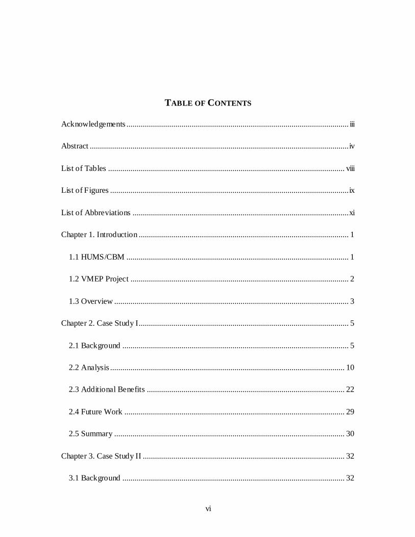
TABLE OF CONTENTS
Acknowledgements ............................................................................................................. iii
Abstract ............................................................................................................................... iv
List of Tables .................................................................................................................... viii
List of Figures ..................................................................................................................... ix
List of Abbreviations .......................................................................................................... xi
Chapter 1. Introduction ....................................................................................................... 1
1.1 HUMS/CBM ............................................................................................................. 1
1.2 VMEP Project ........................................................................................................... 2
1.3 Overview ................................................................................................................... 3
Chapter 2. Case Study I....................................................................................................... 5
2.1 Background ............................................................................................................... 5
2.2 Analysis ................................................................................................................... 10
2.3 Additional Benefits ................................................................................................. 22
2.4 Future Work ............................................................................................................ 29
2.5 Summary ................................................................................................................. 30
Chapter 3. Case Study II ................................................................................................... 32
3.1 Background ............................................................................................................. 32

vii
3.2 Analysis ................................................................................................................... 36
3.3 Summary ................................................................................................................. 57
Chapter 4. Conclusion....................................................................................................... 58
References ......................................................................................................................... 60

viii
LIST OF TABLES
Table 2.1 - Tab Bend and Wedge Equivalence....................................................................9
Table 2.2 - AH-64D Main Rotor Blade Demands for FY09 – FY11 ................................11
Table 2.3 - Projected Peacetime-Reduced Flight Hours as a Percentage of Current Flight Hours ......................................................................................................................12
Table 2.4 - Return on Investment.......................................................................................22
Table 2.5 - UH60 1P/4P Survey & Removal and Replacement Rate Results ...................26
Table 3.1 - Annual T700 Engine Demands for FY12........................................................36
Table 3.2 - Field Repairable Categories.............................................................................38
Table 3.3 - Annual T700 Module Demands for FY12.......................................................42
Table 3.4 - Total MMH for Engine & Field Repairable Categories ..................................53
Table 3.5 - Remaining Field Repairable Categories ..........................................................55

ix
LIST OF FIGURES
Figure 2.1 - Diagram of Main Rotor Blade Tab Bending Tool Operation ..........................6
Figure 2.2 - Photograph of Wedges on an AH-64D Main Rotor Blade ..............................8
Figure 2.3 - Pie Chart of Annual MR Blade Demands and Trailing Edge Failures ..........11
Figure 2.4 - Bar Graph Displaying Material Cost Avoidance Benefit ..............................13
Figure 2.5 - Annual Percentage of Material Cost Avoidance Benefit Achieved ...............14
Figure 2.6 - Phase Cycle for the AH-64D..........................................................................15
Figure 2.7 - Bar Graph Displaying Operational Cost Avoidance Benefit .........................18
Figure 2.8 - Annual Percentage of Operational Cost Avoidance Benefit Achieved .........19
Figure 2.9 - Total Cost Avoidance Benefit Graph .............................................................20
Figure 2.10 - Percentage of ROI Achieved per Year using Material and Operational Cost
Avoidance ..............................................................................................................21 Figure 2.11 - NCARNG AH-64D Wedge Rotor Smoothing Data ....................................23
Figure 2.12 - Comparison of Total Average Failure Rate & MMH/KFH for Top 13 Aircraft Subsystems ...............................................................................................25
Figure 2.13 - Mean Flight Hours Between Failure (MFHBF) vs. Average Aircraft
Propeller Vibration Level.......................................................................................27 Figure 2.14 - Average MMH per FLTHR Before and After Balancing by Aircraft and
Group .....................................................................................................................28
Figure 3.1 - GE T700 Engine Modules..............................................................................35
Figure 3.2 - Pie Chart of Annual Engine Demands and FR Engines Returned to Depot ..38
Figure 3.3 - Money Lost for Each EBR as a Percentage of Weighted Average EBR .......41
Figure 3.4 - ASM SCV and UCV Money Lost Relative to Another .................................43

x
Figure 3.5 - CSM SCV and UCV Money Lost Relative to Another .................................43
Figure 3.6 - GG SCV and UCV Money Lost Relative to Another ....................................44
Figure 3.7 - PTM SCV and UCV Money Lost Relative to Another..................................44
Figure 3.8 - Annual Material Cost Avoidance Benefit for MBR Relative to a Single EBR
Cost ........................................................................................................................46
Figure 3.9 - Annual Material Cost Avoidance Benefit for FR Categories Relative to a Single EBR Cost ....................................................................................................47
Figure 3.10 - Bar Graph Displaying Material Cost Avoidance Benefit ............................48
Figure 3.11 - Annual Percentage of Material Cost Avoidance Benefit Achieved .............49
Figure 3.12 - Material Cost Avoidance Benefit for Specific ASM-Engine
Combinations .........................................................................................................50
Figure 3.13 - Material Cost Avoidance Benefit for Specific CSM-Engine Combinations .........................................................................................................50
Figure 3.14 - Material Cost Avoidance Benefit for Specific GG-Engine Combinations ..51
Figure 3.15 - Material Cost Avoidance Benefit for Specific PTM-Engine Combinations .........................................................................................................51
Figure 3.16 - Total Annual Cost Before & After Maintenance Changes ..........................54
Figure 3.17 - Total Annual Cost Avoidance Benefit by FR Category...............................55

xi
LIST OF ABBREVIATIONS
AED .................................................................................. Aviation Engineering Directorate
AMCOM ............................................................................. Aviation and Missile Command
AMRDEC................ Aviation and Missile Research Development and Engineering Center
ASM ............................................................................................ Accessory Section Module
AUP............................................................................................................. Army Unit Price
AVIM ............................................................................. Aviation Intermediate Maintenance
AVSCOM.........................Army Aviation and Surface Material Command; now AMCOM
AVUM ........................................................................................ Aviation Unit Maintenance
AWCF ...................................................................................... Army Working Capital Fund
AWR .................................................................................................. Airworthiness Release
CBA .....................................................................................................Cost Benefit Analysis
CBM....................................................................................... Condition-Based Maintenance
CCAD........................................................................................ Corpus Christi Army Depot
CCH ................................................................................................. Clogged Cooling Holes
CSM ..................................................................................................... Cold Section Module
DA ................................................................................................... Department of the Army
EBR .............................................................................................Engine-Based Replacement
EPDM...........................................................................Ethylene Propylene Diene Monomer
ERC .....................................................................................................Exit Rub Combination
FEDLOG ............................................................................................Federal Logistics Data

xii
FOD.................................................................................................. Foreign Object Damage
FPG ........................................................................................................ Flight Pitch Ground
FR................................................................................................................. Field Repairable
FY.........................................................................................................................Fiscal Year
GG ....................................................................................Gas Generator Matched Assembly
HUMS ...................................................................... Health and Usage Monitoring Systems
IETM ...................................................................... Interactive Electronic Technical Manual
IMMC.....................................................................Integrated Material Management Center
IPS .............................................................................................................Inches per Second
KTAS .................................................................................. or KTS; Knots, True Air Speed
LMP ................................................................................. Logistics Modernization Program
LRU...................................................................................................Line-Replaceable Units
MAC.......................................................................................Maintenance Allocation Chart
MBR.......................................................................................... Module-Based Replacement
MFHBF ............................................................................ Mean Flight Hours Before Failure
MMH.............................................................................................. Maintenance Man Hours
MMH/KFH................................................. Maintenance Man Hours per 1000 Flight Hours
MR ...................................................................................................................... Main Rotor
MSPU................................................................................... Modern Signal Processing Unit
MTP .................................................................................................. Maintenance Test Pilot
NATC..................................................................................................Naval Air Test Center
NCARNG................................................................... North Carolina Army National Guard
NSN.................................................................................................. National Stock Number

xiii
O&S ................................................................................................. Operations and Support
OSD................................................................................. Office of the Secretary of Defense
PEOAVN ....................................................................... Program Executive Office Aviation
PM .................................................................................................. Project Manager’s Office
PTM .................................................................................................. Power Turbine Module
RIMFIRE ... Remediation/Reliability Improvement thru Failure Identification & Reporting
ROI....................................................................................................... Return on Investment
RS................................................................................................................ Rotor Smoothing
RT&B............................................................................................. Rotor Track and Balance
SCARNG ................................................................... South Carolina Army National Guard
SCV ................................................................................................ Serviceable Credit Value
T/B ...................................................................................................................Track/Balance
TFP........................................................................................................... Test Flight Pattern
UCV ........................................................................................... Unserviceable Credit Value
ULLS-A .................................................................. Unit Level Logistics Support - Aviation
USAF ............................................................................................... United States Air Force
VMEP...........................................................Vibration Management Enhancement Program
VMU ............................................................................................ Vibration Monitoring Unit

1
CHAPTER 1. INTRODUCTION
1.1 HUMS/CBM
In most industries, the Army included, maintenance is performed using a time-
based system. This type of maintenance is best when used with initial designs. After
failures are monitored and data is collected, these scheduled maintenance intervals can be
adjusted. Unfortunately, this method is not ideal as it can lead to unexpected failures in
critical parts, causing operational downtime and potential safety hazards. Due to this, it is
“desirable to consider use-based maintenance practices so that critical parts are replaced
or repaired before their full lifetimes on a variable basis balancing and optimizing both
economic and safe operating conditions” [1]. With improvement to technology and the
increase of the Army’s information infrastructure, many aircraft have been outfitted with
Health and Usage Monitoring Systems (HUMS). With the arrival of these on-board
monitoring systems, maintainers have access to a near real-time assessment of component
health [2]. HUMS utilizes condition-based maintenance (CBM) concepts to minimize
unscheduled failures and maintenance costs. As defined by the Office of the Secretary of
Defense (OSD), CBM is a “set of maintenance processes and capabilities derived, in
large part, from the real-time assessment of weapon system condition obtained from
embedded sensors and/or external tests and measures using portable equipment.” Using
data acquired from HUMS, incipient problems are identified and corrective actions are
taken to improve the reliability, availability, and maintainability of the aircraft [3].

2
1.2 VMEP Project
One type of HUMS employed by the Army was implemented through a project
known as Vibration Management Enhancement Program (VMEP). Via this government-
industry-academia cooperative, the goal was to reduce the number of maintenance test
flights, minimize aircraft operation and support costs, augment aircraft availability, and
increase safety through in-flight vibrations monitoring, on-line data processing and
artificial intelligence based decisions. Within the VMEP system, rotor smoothing (RS)
“as well as vibration collection and surveying are fully supported, including the
monitoring of all sensors for capture of exceedances (high condition indicators)” [4].
Succeeding the implementation of the vibration monitoring unit (VMU) in various
aircraft, the University of South Carolina set out to provide an annual cost savings
analysis of VMEP as well as create a cost benefit analysis (CBA) model through the
correlation of vibration signals and the Unit Level Logistics Support-Aviation (ULLS-A)
database. The CBA model utilizes test flight data from ULLS-A “in order to estimate a
cost savings and recovery of the initial cost of the VMU hardware installation and future
cost savings for the Apache and Blackhawk helicopters” [5]. The model includes cost
variables such as: VMEP investment, test flight hours, cost per flight hour, hours per
flight, number of VMEP helicopters, RS flights, non-RS flights. It also considers non-
tangible variables including: morale, availability, operational flight hours’ gain, mission
aborts, safety, unscheduled maintenance occurrence, and premature parts failure. Non-
tangible benefits were measured by tabulating responses based on an administered
questionnaire. The findings from the results conclude that VMEP increases confidence in
early diagnosis, increases confidence overall, increases attention to and concentration on

3
mission and performance, increases morale, increases the sense of safety, and improves
performance. As of the date the paper was presented, a savings in parts costs of $1.4M
has been achieved as well as a savings in parts cost and operation support of $2.1M.
Mission capability rates were increased through a decrease in maintenance test flights and
an increase in total flight time [5].
1.3 Overview
Above all, CBM efforts provide an overwhelmingly beneficial experience for the
military and any other organization that employs it. This research provides two major
case studies that illustrate the potential for significant payoff accomplished by utilizing
CBM practices. Both cases are introduced with background information relevant to
understanding the existing problems. Following this, the current and proposed
maintenance changes are described. Next, each study details a material and operational
cost avoidance that can be earned by implementing the proposed maintenance
improvements and the resulting benefits that can be realized. Additional benefits are
discussed and suggestions for future work are given. Lastly, the case studies are
summarized to highlight the essential points.
Case Study I is a return on investment (ROI) that analyzes the benefits of the
implementation of elastomeric wedges as vibration control on the Apache (AH-64D)
aircraft. Analysis of the material and operational costs shows that the use of self-adhering
elastomeric trailing edge wedges on the Apache helicopter in main rotor blade tracking
operations will significantly reduce the number of blades damaged by tab bending that
must be repaired at the depot level. Wedge implementation will also allow for a decrease
in the number of test flights and maintenance man hours associated with those flights.

4
Additionally, the wedges will lower aircraft vibration levels. A 10-year ROI is calculated
for projected peacetime flying hours and for the current flying rate. Dollar values and
flight hour optempo have been removed and replaced with percentages or pseudonyms to
comply with the operations security process.
Case Study II examines the maintenance practices regarding the GE T700, T701,
T701C, and T701D turboshaft engine. According to the Aviation and Missile
Command’s (AMCOM) integrated priority list, the turboshaft engine is the number one
cost burden to the Army with Army Working Capital Fund (AWCF) salesc exceeding
$260M for FY12 and projected salesd over $200M for FY13. Analysis of
Remediation/Reliability Improvement through Failure Identification and Reporting
(RIMFIRE) data on engines determined to be field repairable by depot shows return of
engine modules in lieu of the entire engine yields a significant cost avoidance. Returning
modules instead of engines would reduce the number of field repairable engines sent to
depot by almost 50%. Additional ways to reduce the number of field repairable engines
are discussed and their benefits are included. Dollar values and component demand data
have been removed and replaced with percentages or pseudonyms to comply with the
operations security process.
c Total AWCF Sales (last 12 months) is defined as “Dollar value of the AWCF sales for the last 12 mon ths
calculated by multiplying the AMDF price times the number of independent demands”. The AMDF Price
definition states “Also known as the standard price, it includes the latest acquisition cost plus the authorized
cost recovery rate (surcharge)”. Independent Demands are “the demands generated by a funded requisition
from a retail unit”. d Projected AWCF Sales (next 12 months) is defined as “Dollar value of the AWCF sales for the next 12
months calculated by multiplying the AMDF price times the number of fo recasted independent demands
for the next 12 months”.

5
CHAPTER 2. CASE STUDY I
2.1 Background
In 2010, the Vibration Control project began with one goal of improving the main
rotor (MR) blade tracking feature used in helicopter main rotor smoothing. Routinely
scheduled maintenance events use rotor smoothing (RS), also known as rotor track and
balance (RT&B), to make corrective adjustments to pitch links, blade weights, and trim
tabs with the use of Modern Signal Processing Unit (MSPU) equipment and procedures.
Helicopter rotor smoothing is a complex process, requiring precise adjustments to a rotor
system that has many dynamic forces in play [6]. The purpose of these adjustments is to
improve the track of main rotor blades and determine their sensitivities, which reduces
vibrations at the fundamental (once-per-revolution) rotor frequency. Alternatively,
applying main rotor wedges can be used to reduce vibration instead of bending tabs.
Helicopter main rotor wedges can be thought of as a more complex version of a
balancing kit that can be purchased for a ceiling fan with wobbling blades. Reducing
these vibrations increases the “smoothness” of aircraft flight. Lower vibration levels also
result in a reduction in crew fatigue and a service life extension for both the airframe and
installed components [6]. Current maintenance procedures prescribe bending metal tabs,
which extend off the trailing edge of the main rotor blade, to a specified angle [7-9]. Tabs
are bent using a tab bending tool, also known as a trim tab tool. A diagram displaying the
tab bending operation can be seen in Figure 2.1, where KTAS stands for “knots, true
airspeed”, sometimes written KTS.

6
Figure 2.1: Diagram of Main Rotor Blade Tab Bending Tool Operation [10]
2.1.1 Current Procedure: Trim Tab Bending
The trim tabs are effective at achieving acceptable vibration and satisfactory blade
track but put excessive burden on maintainers by requiring several maintenance test
flights for adjustments as well as frequent adjustments over time to maintain low
vibration levels. The trim tab tool only fits in one pocket at a tab so rotor balancing can
get to be time intensive. Furthermore, trim tab adjustment can damage the blade,
requiring blade replacement. In flight, the highest strain levels of any blade location are
experienced along the trailing edge of the main rotor blade [9]. Bending the tab causes
further strain along the bend, resulting in compromised material strength. This
compromised strength means that the metal tab is subject to movement, both over time
and as a result of blade flexing during flight, leading to degradation in rotor track and
vibration [11]. All of this leads to trim tab washout, which means that the blade can no
longer hold the angle required for rotor smoothing. Trim tab washout is a leading cause
of increased vibration values over time. Washout is also experienced due to high gross
weights and high airspeeds [6]. A certain skill is necessary when using the tab bending

7
tool, a skill that is not taught to every maintainer. An inexperienced maintainer could
easily exceed the maximum bend limit of 5° if not properly trained, resulting in blade
damage beyond reparable limits. Consequently, RT&B actions could be delayed by an
absence of trained maintainers. Even if the tab bending process is performed by an
experienced maintainer, “trim tab angles are often applied inconsistently due to the
inherent design of the trim tab bender, trim tab stiffness differences, and individual
maintainer bending techniques” [6]. Repeatability of the angle change is another issue
since the magnitude of the required adjustment is often very small. A limited quantity of
trim tab tools is provided to each unit; therefore, maintenance could also be hindered by a
lack of tool availability. The MR wedges will be implemented to recreate the trim tab’s
success in reducing vibration while decreasing maintenance time and MR blade demand.
2.1.2 Alternative Procedure: Wedges
Boeing designed self-adhering elastomeric wedges to improve the vibration and
blade tracking over the helicopters full speed range while improving the current method
of adjustment in a field environment. The tracking wedges have a peel and stick adhesive
backing and are made of Ethylene Propylene Diene Monomer (EPDM) elastomer, which
was chosen for its high resistance to chemical and environmental exposure. The relatively
soft elastomer with low stiffness offers three major advantages: (1) it significantly
reduces the adhesive demand allowing for the use of a pressure sensitive adhesive system
in lieu of epoxy, which can result in permanent damage to the blade or wedge upon
removal; (2) low stiffness means facilitated removal making the process similar to
peeling tape from a flat surface; (3) to facilitate length adjustment since it can be cut with
hand scissors [11]. Wedge kits include a piece of Scotchbrite pad, two alcohol wipes, and

8
one 10.0-inch long, 1.25-inch wide wedge with a thickness angle taper of 6° [9]. A
photograph of wedges installed on a MR blade can be seen in Figure 2.2.
Figure 2.2: Photograph of Wedges on an AH-64D Main Rotor Blade (Courtesy of 1-
151 ARB)
The addition of discrete main rotor wedges to the trailing edge of the main rotor
blades allows for the same change in lift and pitching moment characteristics of the
airfoils as experienced by trim tab deflection. Another immediate benefit is that flight test
mechanics have found the MR wedge installation to be quicker, easier, and more precise
as compared to bending trim tabs [9]. Moreover, trim tab washout will be eliminated
since the blades are no longer required to be bent to a specific angle. The simple nature of
the wedge design allows for a greater degree of adjustment to vibration and track through
a wider range of airspeed that tab bending cannot provide consistently. It should also be
noted that after accumulating hundreds of hours of flight time on a helicopter, none of the
wedges failed or showed signs of significant peeling. These flight hours were performed

9
on a variety of helicopters at typical speeds and altitudes in a variety of weather
conditions for extended periods of time [11].
MR wedge installation is guided by the instruction of the MSPU system. A simple
correlation is established for the appropriate amount of wedge based on MR trim tab bend
requirements from the MSPU system [9]. The wedge equivalence to tab bends is listed in
the wedge airworthiness release (AWR) and an overall correlation from that document
for wedges and tab bends is shown in Table 2.1.
Table 2.1: Tab Bend and Wedge Equivalence [9]
Tab Bend
(deg.)
Equivalent
Wedge Length
per Pocket (in.)
Total Wedge
Length, Pockets
4-10 (in.)
Total Wedge
Length, Pockets
6-10 (in.)
Total Wedge
Length, Pockets
8-10 (in.)
0.5 1.0 7 5 3
1.0 2.0 14 10 6
1.5 3.0 21 15 9
2.0 4.0 28 20 12
2.5 5.0 35 25 15
3.0 6.0 42 30 18
3.5 7.0 49 35 21
4.0 8.0 56 40 24
4.5 9.0 63 45 27
5.0 10.0 70 50 30
A 3.0° bend in pockets 4-10 would mean that each individual pocket would need
to be bent 3.0°; since the tab bending tool fits only in one pocket at a time, this task will
be time consuming. With wedges, that same 3.0° bend simply means that 42 inches of
wedge must be applied on the blade in pockets 4-10. The wedge AWR explains, “The
shaded areas represent conditions for which there may not be enough real estate for the
wedges. If the adjacent pockets are available, wedges may be added to the pockets
immediately inboard or outboard.”

10
2.2 Analysis
Material and operational costs are examined to ultimately determine the return on
investment after 10 years with the implementation of the MR elastomeric trailing edge
wedges. The projected annual savings, or benefits, determined in the following analyses
are taken as a cost avoidance in that these are costs that will not be spent on maintenance,
but on training or missions. The material cost avoidance explores the costs associated
with main rotor blade demand, while the operational cost avoidance considers the
maintenance-related costs. The ROI incorporates the benefits from both the material and
operational cost avoidances.
2.2.1 Material Cost Avoidance
Material costs are developed from Aviation and Missile Command (AMCOM)
Integrated Material Management Center (IMMC) and Aviation and Missile Research
Development and Engineering Center (AMRDEC) total return and demand data for MR
blades.
2.2.1.1 MR Blade Material Demands FY09 – FY11
The analysis begins by acquiring the total demand for AH-64D MR blades from
FY09 to FY11 which is used to then obtain an average MR blade demand. The values in
Table 2.2 are taken as a percentage of the average annual MR blade demand. The total
demand data for FY09 (60.35%) is significantly lower than the total demand data for
FY10 and FY11 (132.81% and 106.84%, respectively). Due to a changeover in AMCOM
Logistics Modernization Program (LMP) procurement systems, the demand for the entire
FY09 year was not able to be accessed; the demands are only from 14 May 2009 to 20
Sep 2009. These values are not used to create a predicted annual demand due to an

11
abnormal spike in demand during that time. The resulting values from this absence in
data just provide a more conservative value than what would have been determined
otherwise.
Table 2.2: AH-64D Main Rotor Blade Demands for FY09 – FY11 in AMCOM LMPe
Main Rotor Blade
National Stock
Number (NSN)f
FY09 Total MR
Blade Demandg
FY10 Total MR
Blade Demandg
FY11 Total MR
Blade Demandg
MR Blade 1 60% 138% 102%
MR Blade 2 56% 75% 169%
MR Blade 3 72% 116% 112%
MR Blade 4 45% 85% 170%
Total: 60% 133% 107%
2.2.1.2 MR Blade Field Returns to Depot
Based on historical maintenance data, it is implied that trailing edge failures are
related to tab bending. According to the team leader for the Aviation Engineering
Directorate (AED) Maintenance Division at Corpus Christi, TX, the number of blades
that are rejected for damage to the trailing edge beyond reparable limits is equivalent to
35.64% of the average annual MR blade demand.
Figure 2.3: Pie Chart of Annual MR Blade Demands and Trailing Edge Failures
e Values taken as a percentage of the average annual MR blade demand
f CSM Woody Sullivan; Department of the Army (DA) Form 2408 g Sara D. Finigan; AMCOM IMMC Item Manager for MR Blade
Total Average Annual
Main Rotor Blade
Demands
Main Rotor Blade Returns
due to Trailing Edge
Failures (35%)

12
Figure 2.3 is a graphical representation of the MR blades that will be affected by
wedge implementation. The number of MR blades with trailing edge failures will
decrease with the use of wedges and it is what the material costs focus on.
2.2.1.3 Material Costs Prior to Wedge Implementation
Using the average annual MR blade demand, the unit price for the MR blade, and
the percentage of MR blade returns due to trailing edge failures, the material costs prior
to wedge implementation can be calculated. For this analysis, 35% is used for the MR
blade returns that are due to trailing edge failures in order to obtain a more conservative
value.
2.2.1.4 Material Costs After Wedge Implementation
Total flight hours for FY09, FY10, and FY11 are averaged together to find the
current annual flight hour rate. In order to determine the material costs after wedge
implementation, a peacetime estimate of flight hours is considered. It is anticipated that
the United States will not always be at war and this should be reflected in the analysis.
Values used in the subsequent calculations are taken as a peacetime-reduced percentage
of the previously mentioned rate. Table 2.3 lists these projected rates as a percentage of
the current rate.
Table 2.3: Projected Peacetime-Reduced Flight Hours as a Percentage of Current
Flight Hours
Percentage of Reduction
Projected Rate 1 42%
Projected Rate 2 50%
Projected Rate 3 63%
Projected Rate 4 75%
Current Rate 100%

13
It is expected that, with the change from tab bending to wedges, fewer blades will
be returned due to trailing edge failures, resulting in a reduced demand. An estimated
reduced demand rate of 25% is anticipated, another conservative value. The reduced
demand rate means that 75% of that value will remain and will continue to be demanded.
This rate is applied to the annual cost of MR blades due to trailing edge failures along
with the calculated ratios given in Table 2.3. The resulting value is the annual cost of MR
blade returns due to trailing edge failures after wedge implementation.
The annual cost of blade returns due to trailing edge failures after wedge
implementation is proportional to the projected peacetime flight hours. This means that as
flight hours increase, the likelihood of having a trailing edge failure on a MR blade
increases as well.
2.2.1.5 Material Cost Avoidance Benefit & Projected Cash Flow
h
Figure 2.4: Bar Graph Displaying Material Cost Avoidance Benefit
h Values taken as a percentage of the annual cost of MR blade returns due to trailing edge failures before
implementation
42% 50% 63% 75% 100%
0%
10%
20%
30%
40%
50%
60%
70%
80%
90%
100%
Projected Peacetime-Reduced Percentage of Flight Hours
Cost,
as a
percen
tag
eh
Material Cost Avoidance
Benefit
Annual Cost of MR Blade
Returns due to Trailing Edge
Failure (35% of Demands)
Before Implementation
Annual Cost of MR Blade
Returns due to Trailing Edge
Failure After Implementation

14
The material cost avoidance benefit is the difference between the current cost and
the new forecasted cost. The benefits decrease as flight time increases. A graphical
representation of that is shown above in Figure 2.4.
The next step is to use the cost avoidance benefit to calculate the benefits
achieved over a 10-year period of time. The projected cash flow over 10 years is
illustrated on a graph in Figure 2.5. The lines on the graph appear to be nonlinear toward
the end. This is due to the full benefit being achieved in both FY18 and FY19, so
inflation is the only difference between the two.
ij
Figure 2.5: Annual Percentage of Material Cost Avoidance Benefit Achieved
Since the data collected is from FY09 through FY11, it is estimated that the
benefits will not begin until two years after the last set of data acquired. This means that
the benefits begin in FY13. The total benefit will not be seen in its entirety during FY13
but will be seen progressively. An incremental benefit of approximately 16.67% per year
was chosen so that by FY18, a 100% benefit is achieved. These calculations also take
i Projected peacetime-reduced flight hours as a percentage of current flight hours
j Cost per year per flight hour taken as a percentage of current rate material cost avoidance benefit
0%
50%
100%
150%
200%
250%
300%
350%
400%
0 2 4 6 8 10
Cost,
as a
percen
tag
ej
Year
Material Cost Avoidance Benefit Per Year Per Flight Houri
42%
50%
63%
75%
100%

15
into account a 3% inflation rate, which was compounded for single flow, also beginning
in FY13. The inflation equation is mathematically expressed as:
( ) ( )
where is the present single sum, is the future single sum, is the interest per period in
percent, and is the period (beginning in FY13) [12].
2.2.2 Operational Cost Avoidance
Operational costs are determined by using phase maintenance to determine how
much it costs to perform rotor smoothing events before and after wedge implementation.
Based on pilot experience, a reduction in maintenance test flight time is observed. The
additional cost of wedge packets is considered here.
2.2.2.1 Rotor Smoothing Events for Fleet
Figure 2.6: Phase Cycle for the AH-64D
It is difficult to determine the exact number of rotor smoothing events per year
since they must sometimes be performed during unscheduled maintenance events. Phase
Fli
gh
t H
ou
rs/A
ircraft
500 – Test Flight T/B
375 – Test Flight T/B
250 – Test Flight T/B
125 – Test Flight T/B
In Phase

16
maintenance is used to create a baseline allowing a comparison between the before and
after costs. Phase maintenance, when related to aircraft, is a system of scheduled
maintenance events. For the AH-64D, phases occur every 500 flight hours. Rotor
smoothing events are guaranteed at every 125-hour interval within the phase; this is
illustrated in Figure 2.6. T/B stands for “Track/Balance”.
The calculations to determine the number of annual rotor smoothing events is
done on an incremental inspection basis. This means that the number of rotor smoothing
events per month for aircraft is determined for the 500-, 375-, 250-, and 125-flight hour
incremental inspections separately. Those values are added up to determine the total
number of rotor smoothing events per month for the fleet. Once that number is multiplied
by 12 months/year, the annual number of RS events for the fleet is determined. The
results of the calculations are proportional to the projected peacetime flight hours. This
means that with higher annual flight rates, the total number of RS events will increase.
2.2.2.2 Operational Costs Prior to Wedge Implementation
Test flight patterns (TFP) are used in rotor smoothing events. A test flight pattern
is a pre-determined path, or pattern, that is flown by the maintenance test pilot (MTP). In
this case, TFP are performed at the beginning of a RS event and after each set of
adjustments made to the blades in order to confirm those adjustments. TFP take
approximately 15 minutes to complete, or 0.25 hours. On average, 3 TFP are done every
RS event when tab bending is used to track and balance the main rotor blades—one
initial flight and two flights to confirm adjustments. This would be about 45 minutes
every RS event. The operating cost of the AH-64D is used in this calculation. This cost is
unburdened, which means that it does not include maintenance man hours. Using the

17
values mentioned above along with the annual RS events for the fleet, the annual cost of
RS events for the fleet prior to wedge implementation is able to be calculated.
2.2.2.3 Operational Costs After Wedge Implementation
With the implementation of wedges, it is predicted that the number of TFP will be
reduced from 3 to 2 per rotor smoothing event. This can be expected because, as it was
stated previously, wedges allow for a more precise adjustment as compared to trim tabs,
so less TFP are required. Additionally, during initial testing of the wedges, Boeing
determined that the use of the wedges provide “a significant reduction in the number of
iterations that are required to achieve acceptable airframe vibration level” [11]. Instead of
45 minutes of flight time during these events, there will now be only 30 minutes of flight
time. The calculated values result in a 33% reduction in costs.
Since tab bending will no longer be used, the analysis must also take into account
the cost of the wedges as an additional cost. Approximately 3 wedge packets are used
during each rotor smoothing event, which is multiplied by the cost of the packet to
acquire the cost of wedge packets per RS event. Instead of being replaced at every 125-
flight hour interval within the phase, or four times every phase, the wedges are replaced
every 250 flight hours, or twice every phase. This means that the annual rotor smoothing
events for fleet value can be reduced to half of the original number when determining the
annual cost of wedge packets for the fleet; the resulting values are equivalent to almost
9% of the operational costs after wedge implementation.
Although the cost of the wedge packets is a material cost, it is used in the
operational cost calculations because it is dependent on the amount of rotor smoothing
events per year. Adding the annual cost of rotor smoothing events after wedge

18
implementation to the annual cost of the wedge packets for the fleet will yield the annual
cost after wedge implementation.
2.2.2.4 Operational Cost Avoidance Benefit & Projected Cash Flow
The operational cost avoidance benefit is calculated the same way as the material
cost avoidance benefit: the difference between the current cost and the new forecasted
cost. The operational cost avoidance benefit increases as flight time increases, which is
unlike the trend seen in the material cost avoidance benefit. This is because there is a
27% cost avoidance across the board. It can be compared to shopping a sale at a
department store. If everything in the store is 30% off, the customer will have a greater
“savings” when buying a $100 item as compared to buying a $50 item. The same concept
is experienced in this situation. A graphical representation of the operational cost
avoidance benefit values is shown in Figure 2.7.
k
Figure 2.7: Bar Graph Displaying Operational Cost Avoidance Benefit
k Values taken as a percentage of current rate annual cost of RS events for fleet before implementation
42% 50% 63% 75% 100%
0%
20%
40%
60%
80%
100%
120%
Projected Peacetime-Reduced Percentage of Flight Hours
Cost,
as a
percen
tag
ek
Operational Cost Avoidance
Benefit
Annual Cost of RS Events for
Fleet After Improvement +
Annual Cost of Wedge
Packets for Fleet
Annual Cost of RS Events for
Fleet Before Implementation

19
As before, the cost avoidance benefit is used to calculate the benefits achieved
over a 10-year period of time. For consistency, the benefits will not begin until FY13, just
as they did with the material cost avoidance benefit. The total benefit will not be seen in
its entirety during FY13 but will be seen progressively. An incremental benefit of
approximately 16.67% per year was chosen so that by FY18, a 100% benefit would be
achieved. These calculations also take into account a 3% inflation rate, which was
compounded for single flow, also beginning in FY13. The projected cash flow over 10
years is illustrated on a graph in Figure 2.8. The lines on the graph appear to be nonlinear
toward the end. This is due to the full benefit being achieved in both FY18 and FY19, so
inflation is the only difference between the two.
lm
Figure 2.8: Annual Percentage of Operational Cost Avoidance Benefit Achieved
l Projected peacetime-reduced flight hours as a percentage of current flight hours
m Cost per year per flight hour taken as a percentage of current rate operational cost avoidance benefit
0%
20%
40%
60%
80%
100%
120%
140%
0 2 4 6 8 10
Cost,
as a
percen
tag
em
Year
Operational Cost Avoidance Benefit Per Year Per Flight Hourl
42%
50%
63%
75%
100%

20
2.2.3 Total Cost Avoidance Benefit
By adding the material cost avoidance benefit and the operational cost avoidance
benefit, the total cost avoidance benefit is obtained. Figure 2.9 displays the total cost
avoidance benefits for each projected peacetime flight hours broken down by material
and operational cost avoidance benefits. The graph shows that overall the trend is that
benefit decreases with increasing flight time. It also shows that the majority of the benefit
comes from the costs that will no longer be spent on blade demands due to the trailing
edge failures.
n
Figure 2.9: Total Cost Avoidance Benefit Graph
2.2.4 Return on Investment (ROI)
A return on investment is a way to evaluate the efficiency of an investment; the
result is expressed as a percentage or ratio. In this case, it is used to predict the return, or
n Values taken as a percentage of current rate total cost avoidance benefit
0%
50%
100%
150%
200%
250%
42% 50% 63% 75% 100%
Cost,
as a
percen
tag
en
Projected Peacetime-Reduced Percentage of Flight Hours
Operational Cost
Avoidance Benefit
Material Cost
Avoidance Benefit

21
cost avoidance, that will be gained in the future. The formula for determining the ROI is
given as such:
The expense is taken as the total investment in the Vibration Control project. The
first investment is given in FY10. The second investment is given in FY11 and is
equivalent to 53% of the first investment. The final investment is given in FY12 and is
equal to 24% of the first investment. These costs are known as sunk costs because they
have already been incurred and cannot be recovered. The benefit is determined by using
the total cost avoidance. Figure 2.10 illustrates how much of the ROI that is achieved per
year. Table 2.4 displays the return on investment values determined for each assumed
flight hour/month.
o
Figure 2.10: Percentage of ROI Achieved per Year using Material and Operational
Cost Avoidance
o Projected peacetime-reduced flight hours as a percentage of current flight hours
-500%
0%
500%
1000%
1500%
2000%
2500%
0 2 4 6 8 10
Year
ROIo
42%
50%
63%
75%
100%

22
Table 2.4: Return on Investment
Projected
Peacetime-Reduced
Flight Hours
Return on
Investment (ROI)
42% 2300.42%
50% 2114.69%
63% 1832.50%
75% 1550.31%
100% 978.09%
2.3 Additional Benefits
This analysis has demonstrated that elastomeric tracking wedges provide a
substantial amount of benefits. Reducing the time spent on maintenance test flight
patterns also reduces the maintenance man hours (MMH) involved in a rotor smoothing
event. This value is difficult to calculate because the time spent balancing rotor blades
can be vastly different between aircraft. This holds true more so for trim tab bending as
compared to wedges. Discussion with maintenance crew members revealed that the
length of rotor smoothing events using the tab bending tool can range from a couple of
hours to a full work day. This suggests that rotor smoothing events without wedges are a
huge strain on MMH and hinder the availability of the aircraft.
Figure 2.11 is a chart comparing rotor smoothing vibration levels from North
Carolina Army National Guard (NCARNG) and the AH-64D fleet against the Army’s
goal. The NCARNG fleet uses only wedges for rotor smoothing and the rest of the
Army's fleet uses tab bending for rotor smoothing. The data collected is from January
2012 through January 2013. FPG stands for “flight pitch ground” which means there is
no pitch in the blades while on the ground. The vibration is measured in inches per
second (IPS). The first thing to recognize about the chart is that all wedge levels are
below the goal. At FPG and Hover, the wedge vibration average is higher than the fleet

23
average. This is not significant because the majority of flight time is spent from 60 KTS
to 100 KTS, where the wedge average is lower than the fleet average. Overall, it is safe to
say that the use of wedges results in lower vibration levels as compared to vibration
levels experienced by aircraft using tab bending.
Figure 2.11: NCARNG AH-64D Wedge Rotor Smoothing Data, provided by Stanley
H. Graves
According to the AWR for the MSPU [13], “rotor smoothing adjustments
recommended by the MSPU system…may be made without necessitating an additional
maintenance test flight. Relief from the maintenance test flight requirement only applies
if MSPU measured vibration levels are 0.50 IPS or less and the displayed Main Rotor
Smoothing status is green or green with an upward arrow.” When looking at the figure
above, it can be seen that all of the vibration levels from wedge aircraft are far below
0.50 IPS. This means that the number of maintenance test flights can be further reduced
with the use of elastomeric wedges instead of bending tabs.
FPG Hover 60 Kts 80 Kts 100 Kts 120 Kts 140 Kts
NC Wedge Average 0.13 0.17 0.13 0.15 0.18 0.19 0.22
Fleet Average 0.08 0.15 0.14 0.19 0.22 0.25 0.34
Goal 0.20 0.20 0.30 0.30 0.30 0.30 0.30
0.00
0.05
0.10
0.15
0.20
0.25
0.30
0.35
0.40
IPS
AH-64D Wedge Rotor Smoothing Data
NCARNG as of January 5, 2013

24
2.3.1 Examples of Second Order Effects from Lower Vibration Levels
Lower vibration levels can result in a multitude of second order effects. The
results/benefits found in the following examples can be applied to the vibration effects
expected from the AH-64D.
2.3.1.1 Rotor Mounted Bifilar Vibration Absorber Study (1970)
Angelo C. Veca [14] wrote about the vibration effects on helicopter subsystem
reliability, maintainability, and life-cycle costs. The study examines two groups of United
States Air Force (USAF) H-3 helicopters: one equipped with a rotor-mounted bifilar
vibration absorber and one without the absorber. The aircraft were alike in all other
respects. Each group consisted of 15 aircraft each and conducted approximately the same
number of flight hours during the time period covered by the study [14]. The bifilar
vibration absorber reduces helicopter vibration induced by the rotor. The evidence in this
report indicates that a decreasing vibratory stress level from the absorber results in a
decreasing failure rate as well as a significant reduction in direct maintenance. With an
average vibration level reduction of 54.3%, “the overall H-3 helicopter failure rate and
corrective maintenance are reduced by 48% and 38.5%, respectively. Correspondingly,
life-cycle costs show a significant reduction of approximately 10% for the overall
aircraft.” It goes on to state, “The improved reliability resulting from the reduced
vibratory stress environment results in less corrective maintenance being expended on the
H-3 aircraft. This results in less downtime on the aircraft, thereby improving availability
and contributing to the reduction in the operating cost of the aircraft.” Additionally, the
paper concludes that “the reductions are manifested by lessening the costs of direct
maintenance manpower and spares, and by improving helicopter utilization.” Figure 2.12
is a chart from the report displaying a comparison of the total average failure rate and

25
maintenance man-hours per 1000 flight hours (MMH/KFH) for the top 13 aircraft
subsystems. It highlights the “dramatic reduction in both average failure rate and
maintenance man-hours that appears to result from the reduction in vibration.”
Figure 2.12: Comparison of Total Average Failure Rate & MMH/KFH for Top 13
Aircraft Subsystems [14]

26
2.3.1.2 UH-60 Vibration Surveys (1988)
Vibration surveys on the UH-60 aircraft were conducted in 1988 by U.S. Army
Aviation and Surface Material Command’s (AVSCOM, which is AMCOM today)
Aeromechanics. A sample of 9 aircraft from Fort Rucker and 12 aircraft at Fort Campbell
were surveyed. The results showed that the vibration levels for the aircraft at Fort
Campbell were twice that of Fort Rucker’s and are given in Table 2.5. Additionally,
unscheduled maintenance removal and replacement rates were studied. This study found
that Fort Rucker maintained UH-60 aircraft had one-half the removal and replacement
rates of regular Army UH-60 aircraft [15]. The equipment categories that were surveyed
are the following: instruments, avionics, flight controls, and electrical systems.
Table 2.5: UH-60 1P/4P Survey & Removal and Replacement Rate Results [15]
Average Vibration
Levels at 140 Kts Unscheduled
Maintenance Removal
& Replacement Rates 1P 4P
Fort Rucker (Sample of 9 aircraft)
0.2 IPS 0.3 IPS 23 per 1000 flight hours
Fort Campbell
(Sample of 12 aircraft) 0.4 IPS 0.55 IPS 51 per 1000 flight hours
2.3.1.3 Navy P-3 Orion Propeller Dynamic Balancing
Although vibration in a fixed wing aircraft is inherently less severe than in rotary
wing aircraft, reducing the aircraft’s vibration level is still critical to the longevity of its
components [16]. In the early 80s, the propellers of 200 P-3 aircraft were dynamically
balanced. Prior to balancing, the average vibration was 0.40 IPS. After balancing, the
average vibration level dropped to 0.15 IPS. For six months prior to and six months
following the propeller balancing, the Navy tracked the maintenance records of the 200
aircraft for nine selected systems. The Mean Flight Hours Between Failure (MFHBF) for

27
the aircraft with balanced propellers doubled that of the unbalanced propellers. The
results can be seen in Figure 2.13 [17]. Lower vibration levels lead to an increase in
MFHBF for every single system that was monitored, with MFHBF increases ranging
from approximately 90 to 180 hours.
Figure 2.13: Mean Flight Hours Between Failure (MFHBF) vs. Average Aircraft
Propeller Vibration Level [17]
The findings from the study shown above prompted a follow-up study. In the
second study, data was collected from 1,797 dynamically balanced propellers, before and
after the balance. The mean vibration level had decreased from 0.252 IPS to 0.05 IPS and
the standard deviation decreased from 0.158 IPS to 0.042 IPS. Over two years, Nava; Air
Test Center (NATC) followed 15 aircraft and found that the lower vibration levels led to
0
50
100
150
200
250
300
1 2 3 4 5 6 7 8 9 10
Hou
rs
Systems
Mean Flight Hours Between Failure (MFHBF)
vs.
Average Aircraft Propeller Vibration Level
Low IPS
High IPS
1. Reduction Gear Assy. 2. Valve Housing 3. Fuel Leaks/Tanks
4. HF-1 5. VHF Receiver 6. APS-115 Radar
7. ASA-70 Display 8. TD Amplifier 9. Doppler 10. Avg. Of All Sys.

28
a reduction of 11.5% in the MMH per flight hour. Following the second study, it was
decided to implement dynamic balancing procedures [18].
A third study was done to determine the optimum vibration level of the propeller
and the effects of spinner replacement on the propeller’s vibration level. One hypothesis
from this study is that aircraft with propellers dynamically balanced to ≤ 0.10 IPS would
require fewer maintenance man hours per flight hour than aircraft with propellers
balanced to ≤ 0.20 IPS. A squadron of eight aircraft was split into two groups with four
aircraft each—the treatment group and control group. The first group was balanced to ≤
0.10 IPS and the second group was balanced to ≤ 0.20 IPS. The results are shown in
Figure 2.14.
Figure 2.14: Average MMH per FLTHR Before and After Balancing by Aircraft
and Group [16]
The results shown above support the hypothesis that propellers with lower
vibration levels require fewer maintenance man hours per flight hour. It was concluded
0
10
20
30
40
50
SG50 SG51 SG52 SG53 *SG54 *SG55 *SG56 SG57 Group 1 Group 2 All AC
MM
H
per F
LT
HR
Hou
rs
Average MMH per FLTHR Before and After Balancing by
Aircraft and Group
Before
After
* Indicates Group 2 aircraft

29
that the preferred vibration level is ≤ 0.10 IPS for the following reasons: 1) it will prevent
the propeller’s vibration level from exceeding the maximum acceptable level of 0.20 IPS;
2) it reduces the cost of operations by increasing equipment mean flight hours between
failure and reducing the amount of maintenance; 3) little or no additional maintenance
cost was incurred when dynamically balancing the propeller to ≤ 0.10 IPS instead of ≤
0.20 IPS [16].
2.4 Future Work
The AH-64 self-adhering wedges have been modified to fit the H-47 and H-60M
aircraft. Initial testing has been completed for both helicopters leading to a limited AWR
being released for the H-47 and one being expected for the H-60M. Reports from the test
locations indicate that intermediate unscheduled RS events are almost never needed as
the wedges maintain rotor system vibrations at maintenance test flight levels between
maintenance intervals [6]. Users from multiple locations state that wedges are preferred
over the use of trim tabs. These reactions suggest that the use of elastomeric wedges
should be investigated for additional aircraft and would lead to desirable vibration levels.
Wedge equipped and non-wedge equipped aircraft vibration levels will continue
to be monitored. Along with the vibration levels, fuel consumption can be tracked to see
what relations may exist between the two. Reduced vibration will lead to fewer
structural-fatigue-related faults which can be discovered by observing internal
mechanical and electrical components. An increase in mean time between failure and a
reduction in removal and replacement rates is expected as well. The MR blades can be
tracked to observe extended component life and likewise, a reduction in demand. MR

30
trailing edge failures can be monitored to see just how many exist after the introduction
of wedges to maintenance protocol.
2.5 Summary
It is safe to say that elastomeric wedges used on AH-64D main rotor blades are an
improvement in rotor smoothing events over bending the trailing edge metal trim tabs.
Wedges are quicker, easier, and more accurate than bending tabs, for installation and use
over time. This means that maintenance delay due to limited tooling or an absence of
trained maintainers will be eliminated. The wedges provide the same change in lift and
pitching moment characteristics as tab bending. Trim tab washout is not an issue with
wedges since the metal tab is no longer being bent to hold an angle.
Due to the tracking accuracy of the wedges, the maintenance test flight patterns
flown during rotor smoothing events decrease by, on average, one test flight pattern per
event, which results in a 33% reduction in operational test flight pattern hours during
phase maintenance across the entire fleet. The elastomer that the wedges are made from
have a high resistance to chemical and environmental exposure, which means that
wedges only need to be applied every 250-flight hours within the phase instead of every
125-flight hours. Even with the addition of wedges as a cost, a 27% reduction in
operational costs before wedge implementation exists. This value increases as flight time
increases.
It has been demonstrated that the use of tracking wedges will decrease the overall
MR blade demand by reducing the amount of trailing edge failures experienced by main
rotor blades. The material cost avoidance increases as flight time decreases. The majority

31
of the total cost avoidance benefit comes from the blades that will no longer be returned
and demanded due to trailing edge failures.
The use of elastomeric wedges result in lower levels of vibration which leads to
the following benefits: less corrective maintenance actions (and thus, MMH required),
reduced downtime, lowered component failure rate, a reduction in removal and
replacement rates, increased mean time between failure, increased reliability, increased
availability, and increased maintainability. Three out of four Condition Based
Maintenance (CBM) objectives are affected: the soldier and maintenance burden is
reduced, operational support cost is reduced, and aircraft availability is increased.
The analysis of both the material and operational benefits that are achieved from
the use of elastomeric wedges as a form of vibration control result in a 10-year return on
investment of between 9.8:1 and 23:1 for the current rate of flight and a range of
projected peacetime flight hours.

32
CHAPTER 3. CASE STUDY II
3.1 Background
The U.S. government spends hundreds of billions of dollars annually on its
defense budget. Over the past few years, the budget has gradually been reduced. With
these budget cuts, the military must develop new methods of cost avoidance. According
to the Aviation and Missile Command’s (AMCOM) integrated priority list, the turboshaft
engine is the number one cost burden to the Army with Army Working Capital Fund
(AWCF) salesp exceeding $260M for FY13 and projected salesq over $200M for FY14.
Many cost-saving initiatives have been proposed and implemented to optimize operations
and support (O&S) efforts [19]. One effective way to avoid costs is to focus on
maintenance. By increasing the life of components and by streamlining maintenance
processes, the frequency of maintenance events is reduced and costs can be avoided.
3.1.1 Maintenance Levels
The Aviation Maintenance concept for Army aviation defines three maintenance
levels: Aviation Unit Maintenance (AVUM), Aviation Intermediate Maintenance
(AVIM), and Depot Maintenance. The condensed descriptions of each maintenance level
follow.
p Total AWCF Sales (last 12 months) is defined as “Dollar value of the AWCF sales for the last 12 months
calculated by multiplying the AMDF price times the number of independent demands”. The AMDF Price
definition states “Also known as the standard price, it includes the latest acqu isition cost plus the authorized
cost recovery rate (surcharge)”. Independent Demands are “the demands generated by a funded requisition
from a retail unit”. q Projected AWCF Sales (next 12 months) is defined as “Dollar value of the AWCF sales for the next 12
months calculated by multiplying the AMDF price times the number of forecasted independent demands
for the next 12 months”.

33
The lowest level activities, AVUM, are “staffed and equipped to perform high-
frequency ‘On-Aircraft’ maintenance tasks required to maintain a level of aircraft
readiness” [20]. These activities will be governed by the Maintenance Allocation Chart
(MAC) and include basic/minor troubleshooting, replacements, repairs, and other tasks
that do not require extensive or complex adjustments.
As stated by the Interactive Electronic Technical Manual (IETM), AVIM
“provides mobile responsive ‘One-Stop’ maintenance support.” AVIM performs all
maintenance tasks that are authorized to be done at the AVUM level. AVIM can also
repair selected items for return to stock and can determine the serviceability of certain
modules before its expired TBO. All unserviceable repairable modules/components and
end items beyond the capability of AVIM to repair will be evacuated to the third
maintenance level—Depot Maintenance
Depot-level maintenance performs all maintenance tasks that are authorized to be
done at the lower levels as well as “material maintenance or repair requiring the overhaul,
upgrading, or rebuilding of parts, assemblies, or subassemblies, and the testing and
reclamation of equipment as necessary” [21]. For all of the GE T700 turboshaft engines,
which include the T700, T701, T701C, and T701D variations, there is only one depot
location for returns.
3.1.2 Maintenance Process
When it is discovered that a repair or replacement must be made to the engine, the
maintainer utilizes the technical manual. This allows the maintainer to run through
troubleshooting procedures to evaluate the cause of the issue and remediate that issue. If
the repair cannot be performed at the AVIM level, the engine is sent to Corpus Christi
Army Depot (CCAD) in Texas, the only depot location for T700 engine returns. Upon its

34
arrival at CCAD, a tear down analysis is performed on the engine and an inspector
determines if the engine was field repairable (FR). This and many other details related to
each engine are entered into a system called RIMFIRE, which stands for
Remediation/Reliability Improvement through Failure Identification and Reporting.
According to Stephanie Burke, a reliability engineer for RIMFIRE, QuantiTech, Inc., the
definition for FR is “the failure mode or condition that caused the inducted item to be
returned to the depot was determined to be repairable in the field, based on current unit
level maintenance procedures and manuals.” Additionally, the depot-level maintainer
must perform the necessary repairs to the engine so that it can be put back in use.
3.1.3 Engine-Based Replacements vs. Module-Based Replacements
The engines determined to be FR after depot-level inspection can also be referred
to as engine-based replacements (EBR). EBR occur when an entire engine is returned to
depot to maintain fleet availability. This could be due to the inability to discover the root
of the problem. Another reason is that the maintenance action requires module
replacement but a spare is not in stock. In this particular case, the engine would be sent
back to depot and would be replaced with an engine that is in stock. The problem with
this method is that it becomes costly to send an entire engine back when only one module
needs repair. Once at depot, the engine is torn down only to discover that every other
module is in working condition.
The engine, shown in Figure 3.1, consists of four major modules: Accessory
Section Module (ASM), Cold Section Module (CSM), Hot Section Module, and Power
Turbine Module (PTM). When something fails within the modules, limited repairs can be
performed by AVIM-level maintainers, and even less by AVUM-level maintainers. The
alternative to EBR is module-based replacements (MBR). This means that when a

35
particular module needs a repair done at the depot level, only the module is returned
instead of the entire engine. As it is shown later, just below half of the engines that are
sent to depot are determined FR solely because a module replacement would have solved
the issue. MBR are sometimes frowned upon because many units tend to not have the
modules in stock that need replacing. This can be seen as a burden because the module
would need to be shipped to the unit before the engine could be repaired, thus lowering
the aircraft readiness. By adopting the MBR system, the unit would keep new modules in
stock instead of engines. This allows for a reduction in the number of engines sent to
CCAD and would, in turn, reduce the cost burden the engines have on Army Aviation.
Figure 3.1: GE T700 Engine Modules [20]

36
3.2 Analysis
Material and operational costs are examined to ultimately determine the benefits
achieved with the implementation of the proposed maintenance changes. The projected
annual savings, or benefits, determined in the following analyses are taken as a cost
avoidance in that these are costs that will not be spent on maintenance, but on training or
missions. The material cost avoidance explores the costs associated with switching from
engine-based replacements to module-based replacements as well as taking the time to
make certain repairs to the engine in lieu of returning the entire engine. The operational
cost avoidance considers the maintenance man hours (MMH) involved.
3.2.1 Material Cost Avoidance
Material costs are developed from RIMFIRE, the AMCOM Integrated Priority
List for FY12, and Federal Logistics Data (FEDLOG).
3.2.1.1 Engine Demands for FY12
The analysis begins by acquiring the total annual demand for GE T700 series
engines from the FY12 AMCOM Integrated Priority List. This list ranks each component
on its cost burden to the Army. The engines used in this analysis were the only ones with
a demand (independent or dependent) in FY12. Table 3.1 displays each engine with its
rank and its annual demand as a percentage of the entire annual demand.
Table 3.1: Annual T700 Engine Demands for FY12 in AMCOM Integrated Priority
List
Current Rank Nomenclature % of Total Engines
1 Engine A 57.41%
3 Engine B 18.84%
9 Engine C 13.31%
25 Engine D 7.41%
43 Engine E 3.01%

37
3.2.1.2 Percentage of Field Repairable Engines
A dataset was taken from RIMFIRE and includes engines dating from 07 Feb
1990 through 13 Nov 2013. As described previously, when each engine is sent to CCAD,
an inspector performs a tear down analysis on the engine. This includes assessing the
damage and determining whether or not the engine should have been sent to depot or if it
should have been repaired in the field. The engine inspector had the option of marking
the “FR” field “Y” for yes, “N” for no, “N/A” for not applicable, or it could be left blank.
“Y” means that the engine could have been repaired in the field and did not need to be
sent to depot for repair. “N” means that the engine could not have been repaired in the
field and the maintainer was correct in sending the engine to depot for repair. “N/A” is
used when the removal was due to a recap/reset or another directed removal; these types
of removals rarely have a failure or a defect. Because of this definition, “N/A” engines
are considered as not repairable in the field for this analysis and are added in with the
“N” engines.
The ratio of “N” to “Y” engines is applied to the engines with a blank “FR” field
and those engine numbers are added to the “N” and “Y” totals respectively, yielding a
total percentage of FR engines to be 13.91%. It should be noted that the values for FY13
and beyond are incomplete due to the delay in RIMFIRE data entry. The fiscal year for
2013 extends from 1 Oct 2012 through 20 Sep 2013; this FY designation will be used
respective to each year.
Figure 3.2 is a graphical representation of the engines that are determined to be
FR by the inspector at CCAD. It is important to determine the percentage of FR engines

38
of the annual engine demand because it is the value that will decrease with the
implementation of the proposed changes and it is what the material costs focus on.
Figure 3.2: Pie Chart of Annual Engine Demands and FR Engines Returned to
Depot
3.2.1.3 Field Repairable Engine Categories
Along with determining whether an engine is FR or not, the inspector also types
up his or her comments and suggestions for every engine. Each of these comments was
read and every FR engine was categorized by the inspector’s assessment. The categories
as well as their respective percentages (out of the 13.91%) are displayed below in Table
3.2. The bolded categories are the ones that could be quantified by a predetermined repair
or solution given in the MAC; the unbolded categories will be discussed in a later section.
Table 3.2: Field Repairable Categories
Airfoils 23.88%
Clogged Cooling Holes (CCH) 0.59%
Compressor Stall 3.85%
Exit Rub Combination (ERC) 1.63%
Inserts, Studs, Bolts 4.59%
Leak 2.37%
Other 5.63%
Replacement 3.26%
Replacement – Accessory Section Module (ASM) 2.81%
Replacement – Combination 4.59%
Replacement – Cold Section Module (CSM) 36.94%
Replacement – Gas Generator (GG) Matched Assembly 2.37%
Replacement – Power Turbine Module (PTM) 7.41%
Total Annual Engine
Demands Not
Repairable in the Field
Field Repairable
Engines turned in to
Depot Annually
(13.91%)

39
The “Airfoils”, “Clogged Cooling Holes”, and “Exit Rub Combination”
categories refer to engines where the only cost associated with their repair is tied to
MMH. The solution for clogged cooling holes is simply to clean out the holes. It is a
fairly simple procedure. “Airfoils” refer to foreign object damage (FOD) or erosion to the
compressor blades within the CSM. This type of repair is time extensive, but it leads to
component life extension. This type of repair is resolved by trimming and blending the
airfoils. Engines categorized by “Exit Rub Combination” are those with impeller/shroud
exit rub and FOD/erosion to the compressor blades. In addition to the airfoil repair, these
engines must also have the exit rub blended.
The remaining bolded categories (Replacement – ASM, CSM, GG Matched
Assembly, PTM) are the module-based replacements. This means that the engine was
determined FR because only the module should have been returned. For these categories,
the analysis does not look at the repairs that can be done to each module upon its arrival
to depot because it assumes that all remaining repairs can only be performed by depot-
level maintainers, hence why it was returned to depot. The GG Matched Assembly is part
of the Hot Section Module and is one of the few repairs that can be made by AVIM-level
maintainers to the interior of the modules.
3.2.1.4 Material Costs Before: Engine-Based Replacements (EBR)
The annual engine demand for FY12 was multiplied by the 13.91% of the engine
demand that were determined to be FR. This yielded the actual number of engines that
would be affected on a yearly basis by improvements to the maintenance process to
decrease the number of FR engines. This number is then multiplied by the percentage of a
single field repairable category, as given in Table 3.2. Since each repair from Table 3.2

40
requires a different cost analysis, a material cost is determined separately for each
category. For example, if the “Clogged Cooling Holes” category is being examined, the
way to discover the number of engines determined FR by repairing CCH is the annual
engine demand for FY12 multiplied by the 13.91% of the engine demand that were
determined to be FR multiplied by 0.59%, which is the percentage of FR engines
categorized as CCH. This equation will be how the base engine number (number of
engines affected) is calculated for each FR category; it will also be used in the following
section.
Now that the number of engines affected can be determined, the cost must be
applied. FEDLOG was used to obtain the Army Unit Price (AUP) and the Serviceable
Credit Value (SCV) of the engine. The AUP is the standard price of the unit and the SCV
is the credit amount for the turn-in of a serviceable item. Using the demands for engines
A-E, a weighted average value was determined for the AUP and SCV. The weighted
average simplifies the analysis by creating a single AUP and SCV for the engine and it
weights each engine’s cost relative to its annual demand. The difference between AUP
and SCV is the sunk cost, or money lost, every time a serviceable engine is returned to
depot.
Figure 3.3 shows the money lost for each EBR taken as a percentage of the
weighted average money lost for EBR. The thick black line designates where the
weighted average money lost for EBR is relative to the individual engines. It can be seen
that Engine C and Engine E are the largest sources for money lost for EBR.

41
Figure 3.3: Money Lost for Each EBR as a Percentage of Weighted Average EBR
3.2.1.5 Material Costs After: Module-Based Replacements (MBR)
The only FR categories with material costs associated with them are the MBR.
Looking back at Table 3.2, it can be seen that almost 50% of the FR engines are due to
MBR. This is significant because by switching to MBR from EBR, over half of the FR
engines will no longer be sent to depot unnecessarily.
The total number of each module demanded annually was taken from the
AMCOM Integrated Priority List. This list ranks each component on its cost burden to
the Army. The modules used in this analysis were the only ones with a demand in FY12.
Similar to the engine demand, these demand values will be used to calculate weighted
average costs for each module. Table 3.3 displays each module with its rank and its
annual demand as a percentage of the entire annual demand per module.
0%
50%
100%
150%
200%
250%
300%
350%
400%
450%
Engine A Engine B Engine C Engine D Engine E
% o
f W
eig
hte
d A
verag
e $
Lost
for E
BR

42
Table 3.3: Annual T700 Module Demands for FY12 in AMCOM Integrated Priority
List
Current Rank Nomenclature % of Total Module
185 ASM A 87.23% 933 ASM B 12.76%
4 CSM A 86.10%
53 CSM B 13.89%
11 GG A 69.73%
173 GG B 9.86% 281 GG C 2.24% 542 GG D 9.64%
2274 GG E 8.52%
13 PTM A 78.41% 89 PTM B 21.58%
FEDLOG was used to acquire the costs involved with the modules. The AUP and
SCV were obtained for each module as well as a third cost: Unserviceable Credit Value
(UCV). The UCV is the credit amount for the turn-in of an unserviceable item. Using the
demands for the separate modules, a weighted average value was determined for the
AUP, SCV, and UCV. Again, the weighted average simplifies the analysis by creating a
single AUP, SCV, and UCV for the modules and it weights each individual module’s cost
relative to its annual demand as part of its respective module. The difference between
AUP and SCV here is the money lost every time a serviceable module is returned to
depot. Similarly, the difference between AUP and UCV is the money lost every time an
unserviceable module is returned to depot. Graphs displaying the difference in money
lost between SCV and UCV for each module are given below in Figures 3.4-7. These
graphs highlight the large difference between the two values for each module.

43
Figure 3.4: ASM SCV and UCV Money Lost Relative to Another
Figure 3.5: CSM SCV and UCV Money Lost Relative to Another
0%
20%
40%
60%
80%
100%
0%
50%
100%
150%
200%
250%
300%
350%
400%
SCV UCV
% R
ela
tive
to
Weig
hte
d A
verag
e A
SM
UC
V M
on
ey
Lost
% R
ela
tive
to
Weig
hte
d A
verag
e A
SM
SC
V M
on
ey
Lost
ASM A
ASM B
0%
20%
40%
60%
80%
100%
0%
100%
200%
300%
400%
500%
600%
SCV UCV
% R
ela
tive
to
Weig
hte
d A
verag
e C
SM
UC
V M
on
ey
Lost
% R
ela
tive
to
Weig
hte
d A
verag
e C
SM
SC
V M
on
ey
Lost
CSM A
CSM B

44
Figure 3.6: GG SCV and UCV Money Lost Relative to Another
Figure 3.7: PTM SCV and UCV Money Lost Relative to Another
0%
20%
40%
60%
80%
100%
120%
140%
0%
100%
200%
300%
400%
500%
600%
700%
800%
SCV UCV
% R
ela
tive
to
Weig
hte
d A
verag
e G
G U
CV
M
on
ey
Lost
% R
ela
tive
to
Weig
hte
d A
verag
e G
G S
CV
Mon
ey
Lost
GG 1
GG 2
GG 3
GG 4
GG 5
0%
20%
40%
60%
80%
100%
0%
100%
200%
300%
400%
500%
600%
SCV UCV
% R
ela
tive
to
Weig
hte
d A
verag
e P
TM
U
CV
M
on
ey
Lost
% R
ela
tive
to
Weig
hte
d A
verag
e P
TM
S
CV
Mon
ey
Lost
PTM A
PTM B

45
With EBR, all engines determined FR are inherently SCV since at least one part
of that engine is serviceable. Yet with MBR, the modules may end up being SCV or
UCV. The SCV and UCV came from the stock on hand values given in the AMCOM
Integrated Priority List. These numbers were made into percentages and applied to each
module to calculate the number of modules that would be determined SCV or UCV upon
the CCAD inspector’s analysis. This part of the analysis does not look at the repairs that
can be done to each module upon its arrival to depot because it assumes that all
remaining repairs can only be performed by depot-level maintainers, hence why it was
returned to depot.
As it was explained in Section 3.2.1.4, the number of engines affected by each FR
category can be determined by multiplying the annual engine demand for FY12 by the
13.91% of the engines that were determined FR and also by the FR category percentage
from Table 3.2. For MBR, this number is used to find the annual money lost every time a
serviceable module or unserviceable module is returned to depot. Again, the money lost
is a sunk cost and it will be incurred every single time a module is returned to depot. In
order to determine the annual money lost due to SCV module returns, the number of
engines affected by each FR category is multiplied by the percentage of SCV for that
specific module and multiplied by the money lost every time that SCV module is returned
to depot. The process is the same to determine the annual money lost due to UCV module
returns, but uses the UCV percentage and UCV money lost per module. The annual
money lost for SCV and UCV are added together to determine the total money lost
annually when returning a particular module to depot.

46
For example, if this analysis is being done for the ASM, the annual engine
demand for FY12 would be multiplied by 13.91% of engines determined FR and also
multiplied by 2.81% to get the number of engines affected by ASM replacement. The
weighted average difference between AUP and SCV would be calculated as well as the
weighted average difference between AUP and UCV. The number of engines affected by
ASM replacement would be multiplied by the percentage of ASM that are SCV and then
by the weighted average difference between AUP and SCV to yield the annual money
lost due to SCV ASM returns to depot. This value would be added to the annual money
lost due to UCV ASM returns to depot to get the total money lost annually when
returning ASM to depot.
3.2.1.6 Material Cost Avoidance Benefit & Projected Cash Flowr
The material cost avoidance benefit is the difference between the current cost
(EBR) and the new forecasted cost (MBR). Figure 3.8 shows the material cost avoidance
benefit annually for each module relative to the cost of returning a single engine to depot.
Figure 3.8: Annual Material Cost Avoidance Benefit for MBR Relative to a Single
EBR Cost
r Cash flow as used in this section refers to cash saved through material cost avoidance as explained herein
-100%
0%
100%
200%
300%
400%
500%
600%
700%
ASM CSM GG PTM

47
The only module with a loss is the CSM; alternatives to this outlier will be described in
the following section. Even so, the annual money lost for sending in CSM over engines
are about half of what it would cost to send in a single FR engine.
As mentioned previously, the first 3 bolded FR categories from Table 3.2 do not
have material costs associated with them. Since these repairs will be performed instead of
EBR, a material cost avoidance benefit exists. So, the new forecasted cost for these 3
categories is $0. Figure 3.9 shows the material cost avoidance benefit annually for each
of the FR categories calculated. Similar to Figure 3.8, each FR category value is taken
relative to the cost of returning a single engine to depot.
Figure 3.9: Annual Material Cost Avoidance Benefit for FR Categories Relative to a
Single EBR Cost
Figure 3.10 displays the material cost avoidance benefit for each module along
with its current and forecasted cost. This graph shows exactly how much of each EBR
cost will be avoided by switching to MBR.
-500%
0%
500%
1000%
1500%
2000%
2500%
3000%
ASM CSM GG PTM Airfoil CCH ERC
ASM
CSM
GG
PTM
Airfoil
CCH
ERC

48
Figure 3.10: Bar Graph Displaying Material Cost Avoidance Benefit
The next step is to use the cost avoidance benefit to calculate the benefits
achieved over a 10-year period of time. It is expected that the total benefit will not be
seen in its entirety during Y1 but will be seen progressively. An incremental benefit of
approximately 11.11% per year was chosen so that by Y10, a 100% benefit is achieved
and engines will no longer be returned to depot in lieu of modules or other repairs. These
calculations also take into account a 3% inflation rate, which was compounded for single
flow, beginning in Y2. The inflation equation is mathematically expressed as:
( ) ( )
where is the present single sum, is the future single sum, is the interest per period in
percent, and is the period (beginning in Y1) [12]. The projected cash flows over 10
years is illustrated on a graph in Figure 3.11. The graph shows exactly how much of each
repair’s material cost avoidance benefit make up the total material cost avoidance benefit
s Cash flow as used in this section refers to cash saved through material cost avoidance as explained herein
ASM CSM GG PTM
-10%
0%
10%
20%
30%
40%
50%
60%
70%
80%
90%
100%
Annual $ Lost EBR
Annual $ Lost MBR
Material Cost Avoidance
Benefit

49
annually. These values are shown relative to the total material cost avoidance benefit
calculated, allowing the total to be exceeded in Y9 due to inflation.
Figure 3.11: Annual Percentage of Material Cost Avoidance Benefit Achieved
3.2.1.7 Examining Specific Engine-Module Combinations
The utilization of weighted averages for the engines and modules allows the
analysis to be simplified. Unfortunately, it does not show the material cost avoidance
benefit of each combination of engine and module. As it was seen in Figure 3.3, these
costs can vary greatly. Taking this into account, the analysis was executed again for every
combination to highlight exactly the benefits that would be achieved with each set. Each
material cost avoidance benefit combination is taken relative to the absolute value of the
weighted average material cost avoidance benefit for each module. Using the absolute
value allows any negative individual material cost avoidance benefit combinations to
remain negative. Graphs illustrating this are shown below in Figures 3.12-15.
-20%
0%
20%
40%
60%
80%
100%
120%
140%
Y1 Y2 Y3 Y4 Y5 Y6 Y7 Y8 Y9 Y10
ERC
CCH
Airfoil
PTM
GG
CSM
ASM

50
Figure 3.12: Material Cost Avoidance Benefit for Specific ASM-Engine
Combinations
Figure 3.13: Material Cost Avoidance Benefit for Specific CSM-Engine
Combinations
0%
50%
100%
150%
200%
250%
300%
350%
400%
450%
500%
Engine A Engine B Engine C Engine D Engine E
ASM A
ASM B
-10000%
-5000%
0%
5000%
10000%
15000%
20000%
25000%
30000%
Engine A Engine B Engine C Engine D Engine E
CSM A
CSM B

51
Figure 3.14: Material Cost Avoidance Benefit for Specific GG-Engine Combinations
Figure 3.15: Material Cost Avoidance Benefit for Specific PTM-Engine
Combinations
-100%
0%
100%
200%
300%
400%
500%
600%
700%
Engine A Engine B Engine C Engine D Engine E
GG A
GG B
GG C
GG D
GG E
0%
100%
200%
300%
400%
500%
600%
Engine A Engine B Engine C Engine D Engine E
PTM A
PTM B

52
Looking at Figures 3.12 and 3.15, it can be seen that all of the values are positive. This
means that for every engine-module combination, costs will be avoided by switching to
MBR from EBR. Out of the 25 possible combinations in Figure 3.14, only Engine D and
GG A yielded a negative material cost avoidance benefit. This one combination situation
represents an insignificant additional cost in light of the overall material cost avoidance
benefits in the 24 other possible combinations. Nonetheless, it should be noted that if a
maintainer comes across a GG A and Engine D combination, it would be better to go
ahead and replace the entire engine.
In Figure 3.13, 4 out of 10 possible combinations resulted in a negative material
cost avoidance benefit. For these combinations, it is more cost efficient to send in the
engine instead of sending in the CSM. It is recommended that the maintainer refer to
these combinations when dealing with a depot-level CSM repair. As it can be seen with
Engines C and E, these MBR yield a very high material cost avoidance benefit.
3.2.2 Operational Cost Avoidance
One major opposition to implementing MBR and emphasizing focus on the other
repairs instead of just returning the engine to depot is the amount of time these repairs
take. The only time that would be saved would be immediate. All of these repairs will
eventually need to be made; the only difference is whether they are being made in the
field or at depot. Returning the engines simply to have less downtime is not necessarily
the best option, barring mission critical situations. Overall, it ends up costing more.
Secondary costs include those incurred by Army Supply; people working in this
department have to file the paperwork and send the engine out. Transportation fees are
increased because the engine weighs significantly more than each module. Moving the
engine across the country, and sometimes overseas, leaves potential for incurred damages

53
along the way. Labor costs are increased because the original maintainers took the engine
apart and put it back together just to have the same process repeated once it arrives at
depot. Furthermore, it is likely that since depot-level maintainers have a higher level of
training that they also have a higher salary. It would be more cost effective to have a
lower level maintainer perform the repairs.
As a reference, the MMH for the engine and FR categories are given below in
Table 3.4. The engine replacement is the only maintenance action that can be done by an
AVUM-level maintainer; all others are AVIM-level.
Table 3.4: Total MMH for Engine & Field Repairable Categories
Component/Assembly Maintenance Function Total MMH
Engine Replace 2.0
ASM Replace 2.7
CSM Replace 4.7
GG Replace 4.8
PTM Replace 3.3
Airfoils Repair 9.5 – 12.7
CCH Repair 6.8
ERC Repair 11.5 – 14.7
According to the MAC, an engine replacement should take 2 hours. Since every other
maintenance action listed requires engine removal, 2.0 hours has been added to each
MMH total. ASM, CSM, and PTM replacement times are comprised of the MMH given
for its specific module replacement as well as the 2.0 hours for engine removal. Since the
GG Matched Assembly cannot be accessed without first removing the PTM, its total
MMH includes engine replacement, PTM replacement, and replacing the GG Matched
Assembly, which consists of the GG stator and stages 1 and 2 GG turbine rotor. As stated
previously, the airfoils are within the CSM so its MMH total includes engine removal,
CSM removal, and airfoil repair. CCH and ERC have estimated MMH. Since ETC

54
consists of engines that need both exit rub blending and airfoil repair, the MMH for both
are included. Exit rub blending is estimated at 2.0 hours. CCH are experienced in the GG
Matched Assembly so an estimated 2.0 hours is added to the GG Matched Assembly total
MMH.
3.2.3 Total Cost Avoidance Benefit
Typically, the total cost avoidance benefit is obtained by adding the material cost
avoidance benefit and the operational cost avoidance benefit together. Since this analysis
consists only of material cost avoidance benefit, that is what the total cost avoidance
benefit will be. Figure 3.16 below displays the total annual costs before (EBR) and after
(MBR) the maintenance protocol changes. Each cost is taken relative to the total annual
cost before in order to highlight the cost avoidance achieved annually.
Figure 3.16: Total Annual Cost Before & After Maintenance Changes
Total Annual Cost Before Total Annual Cost After
0%
20%
40%
60%
80%
100%
120%
Annual EBR Material Cost
Annual ERC Material Cost
(0%)
Annual CCH Material Cost
(0%)
Annual Airfoils Material Cost
(0%)
Annual PTM Material Cost
(2.02%)
Annual GG Material Cost
(0.99%)
Annual CSM Material Cost
(49.54%)
Annual ASM Material Cost
(0.38%)

55
As illustrated in Figure 3.16, the annual cost has been reduced by 47%.
Additionally, the number of engines determined to be FR is reduced by over 75%. In
other words, previously 13.91% of engines demanded annually were determined FR but
with these changes, only 3.39% of engines are determined FR. Ways to reduce this
number even more are discussed in the following section.
Figure 3.17 displays how much each FR category’s total cost avoidance benefit
comprises the total annual cost avoidance benefit.
Figure 3.17: Total Annual Cost Avoidance Benefit by FR Category
3.2.4 Discussion of Other Field Repairable Categories
The analysis thus far has covered 7 out of the 13 FR categories given in Table 3.2.
As a reference, the remaining 6 categories and their percentages of all FR engines are
given below in Table 3.5 so that they can be examined closer.
Table 3.5: Remaining Field Repairable Categories
Compressor Stall 3.85%
Inserts, Studs, Bolts 4.59%
Leak 2.37%
Other 5.63%
Replacement 3.26%
Replacement – Combination 4.59%
ASM, 7.09% CSM, -1.47%
GG, 4.54%
PTM, 16.51%
Airfoil,
67.11%
CCH, 1.65%
ERC, 4.57%

56
Compressor stalls tend to be related to the control system and/or airbleed system.
In order to resolve this issue, the maintainer should have followed troubleshooting
procedures. The troubleshooting procedures lead to the replacement of certain LRUs.
LRUs are line-replaceable units. This repair was not included in the analysis because
troubleshooting should have been done in order to determine which LRU replacements
were needed.
Engines returned to depot under the FR category “Inserts, Studs, Bolts” needed
very simple repairs—to replace the insert, stud, or bolt that was missing from the
assembly. All of these engines were determined to have nothing wrong with them aside
from a small missing part. Installing a replacement part for each of these engines would
have taken no more than 15 minutes.
The only solution for engines with leaks is troubleshooting. This would have led
the maintainer to a maintenance action that could have been taken, most likely involving
a part replacement. Engines within the category of “Other” are those with difficult-to-
determine solutions based on the depot inspector’s notes. The engines labeled
“Replacement” are engines requiring minor AVUM or AVIM-level part replacements;
many of these require LRU replacements. Lastly, the “Replacement – Combination”
category includes engines that require more than one part replacement. This can mean
multiple module replacements and/or replacements of a smaller nature.
Overall, each of these categories would likely result in a positive cost avoidance
benefit. For the purposes of this analysis, the benefits are considered negligible and are
not included.

57
3.3 Summary
It is evident that switching to module-based replacements from engine-based
replacements will reduce the number of engines that are sent unnecessarily to the Army
depot annually. EBR may seem to be more efficient as an immediate solution but in the
long run, it is a massive cost burden. The maintenance burden moves from the more
costly depot-level maintainer to the AVUM- or AVIM-level maintainer. Operations and
support costs are reduced because modules are being returned to depot instead of the
much larger engine. Keeping a higher stock of modules instead of engines allows aircraft
readiness to remain high while avoiding unnecessary costs. To put it into perspective
(based on the weighted average AUP of each engine or engine module), the cost of one
new engine is equivalent to 7.65 ASM, 1.94 CSM, 5.90 GG, or 4.00 PTM.
Another way to reduce the number of FR engines sent to depot is to reassign
certain depot-level tasks to lower maintenance levels. This would further reduce the
operations and support costs and would allow AVUM- and AVIM-level maintainers to
repair more engines and/or modules in-house rather than shipping them to CCAD.
Currently, 13.91% of engines demanded annually are sent to depot with repairs
that could have been made in the field. By replacing modules instead of engines, this
value can be cut in half. After implementing the other maintenance changes detailed, this
number can be reduced even more to 3.39%. As a result, the annual cost of sending
components to depot is reduced by 47%. With the turboshaft engine being the number
one cost burden to the Army, this cost avoidance would be a significant achievement.

58
CHAPTER 4. CONCLUSION
The proposed research effectively demonstrates the various benefits that can be
attained through condition-based maintenance practices. Through the ever-evolving
world of technology, it is important to continually make changes to maintenance
protocols. CBA methods can be applied to various situations to visualize the prospective
gains that can be achieved through adjustments and improvements to current procedures.
Case Study I demonstrates the advantages to self-adhering elastomeric blade
wedges over the current method of trim tab bending in rotor smoothing events. Not only
do they maintain the same change in lift and pitching moment characteristics, but they
also eliminate trim tab washout as a trailing edge failure. Wedges are quicker, easier and
more accurate than bending metal tabs, for installation and use over time. Maintenance
delay due to an absence of necessary equipment or trained maintainers is no longer an
issue. The reduction in trailing edge failures experienced by main rotor blades leads to a
decrease in overall main rotor blade demand. The demand decrease, as a material cost
avoidance, comprises the majority of the total cost avoidance benefit. Due to the tracking
accuracy of the wedges, maintenance test flight patterns flown during rotor smoothing
events are reduced. The favorable material properties of the elastomer prevent the wedges
from degradation during flight. Aircraft equipped with tracking wedges experience lower
levels of vibration leading to the following benefits: less corrective maintenance actions,
reduced downtime, lowered component failure rate, a reduction in removal and
replacement rates, increased mean time between failure, increased reliability, increased

59
availability, and increased maintainability. The analysis of both the material and
operational benefits that are achieved from the use of elastomeric wedges as a form of
vibration control result in a 10-year return on investment of between 9.8:1 and 23:1 for
the current rate of flight and a range of projected peacetime flight hours.
Case Study II explores the benefits to module-based replacement and other
changes to maintenance practices over engine-based replacement. The total cost
avoidance benefit derives solely from the reduction of engines unnecessarily being sent to
Army depot. Maintaining a higher stock of modules instead of engines prevents the
impulse to return the entire engine to depot in order to maintain aircraft readiness. It
allows the readiness to remain high while avoiding unnecessary costs. Reassigning
certain depot-level tasks to lower maintenance levels would reduce the number of field
repairable engines sent to depot. O&S costs would be reduced by keeping more
engine/module repairs in-house rather than shipping the components to CCAD for repair.
Currently, 13.91% of engines demanded annually are sent to depot with repairs that could
have been made in the field. By replacing modules instead of engines, this value can be
cut in half. After implementing the other maintenance changes defined, this number can
be reduced even more to 3.39%. As a result, the annual cost of sending components to
depot is reduced by 47%. With the turboshaft engine being the number one cost burden to
the Army, this cost avoidance would be a significant achievement.

60
REFERENCES
[1] D. Coats. “Comprehensive Joint Time-Frequency Analysis toward Condition Based
Maintenance Regimes for Electrical and Mechanical Components,” Master thesis,
University of South Carolina, Columbia, SC, July 2012.
[2] J. Lawler, L. Potts, E. Hurst. “Reliability Centered Maintenance Analysis of the UH-
60 Drive Train System,” AHS Annual Forum, Huntsville, AL, February 10-11, 2009.
[3] R. K. Mobley. An Introduction to Predictive Maintenance, 2nd ed., Oxford:
Butterworth-Heinemann, 2002.
[4] V. Giurgiutiu, P. Grabill, D. Wroblewski, L. Grant. “Helicopter Health Monitoring
and Failure Prevention Through Vibration Management Enhancement Program,” 54th
Meeting of the Society for Machinery Failure Prevention Technology, Virginia
Beach, VA, May 1-4, 2000.
[5] A. Bayoumi, W. Ranson, L. Eisner, L. Grant. “Cost and Effectiveness of the AH-64
and UH-60 On-Board Vibrations Monitoring System,” Aerospace Conference –
IEEE, Big Sky, MT, March 2005.
[6] J. L. Hunt, R. Bednarczyk, and S. Graves. “Simplifying the Rotor Smoothing Process
in a Military Operations Environment,” AHS 69th Annual Forum, Phoenix, AZ, May
21-23, 2013.
[7] N. A. Miller. “A Comparison of Main Rotor Smoothing Adjustments Using Linear
and Neural Network Algorithms,” Master thesis, Air Force Institute of Technology,
Wright-Patterson Air Force Base, OH, 2006.
61
[8] J. C. Hasty, J. A. Keller and S. M. Krick. “Improved Rotor Smoothing for the U.S.
Army CH-47D,” AHS International Technical Specialists Meeting on Condition-
Based Maintenance, Huntsville, AL, February 2008.
[9] W. D. Lewis. Airworthiness Release (AWR) for Operation of Apache AH-64D
Helicopters with Self-Adhering Elastomeric Trailing Edge Wedges Installed on Main
Rotor Blades (TTS 70805B). Department of the Army: Aviation and Missile
Research, Development, and Engineering Center, Redstone Arsenal, AL, May 10
2010.
[10] AH-64D Smart Book, The Hangar Inc. the Aviator’s Shoppe.
[11] R. T. Loftus and M. J. McNulty. Field Installable and Removable Helicopter Rotor
Blade Vibration and Blade Tracking Device. Patent US 2010/0028151 A1. February
4, 2010. Print.
[12] W. G. Sullivan, E. M. Wicks and J. T. Luxhoj. Engineering Economy, 12 ed., Upper
Saddle River, New Jersey: Pearson Education Inc., 2003.
[13] W. D. Lewis. Airworthiness Release (AWR) for the Modernized Signal Processing
Unit (MSPU) on the AH-64D Apache Helicopter (TTS 77094), Redstone Arsenal,
AL: Department of the Army: Aviation and Missile Research, Development, and
Engineering Center, Dec. 11, 2009.
[14] A. C. Veca. Vibration Effects on Helicopter Reliability and Maintainability, Fort
Eustis, VA: U. S. Army Air Mobility Research and Development Laboratory, April
1973.
[15] S. T. Crews. Helicopter Vibration and its Effect on Operating Costs and
Maintenance Requirements, Huntsville, AL: AMCOM, 1991.

62
[16] L. M. Dew. Propeller Dynamic Balancing’s Effect on Maintenance Manhours Per
Flight Hour for the P-3 Orion, Mar. 10, 1992.
[17] S. Crews. “Rotorcraft Vibration Criteria: A New Perspective,” American Helicopter
Society Forum, May 1987.
[18] Naval Air Test Center (NATC). 54H60 Propeller Balancing Update Brief. Hamilton
Standard Component Improvement Program, June 23-24, 1987.
[19] M. C. Carter. “Post Implementation CBM Benefit Analysis – U. S. Army AH-64D
Apache Helicopter Main Transmission Accessory Sprag Clutch Endurance Project,”
Annual Conference of the Prognostics and Health Management Society, New
Orleans, LA, October 14-17, 2013.
[20] U. S. Army Interactive Electronic Technical Manual (IETM).
[21] 10 U. S. Code § 2460.