Cost Analysis and Estimation Chapter 8. Chapter 8 OVERVIEW Economic and Accounting Costs Role of...
24
Cost Analysis and Estimation Chapter 8
-
Upload
katrina-horn -
Category
Documents
-
view
221 -
download
2
Transcript of Cost Analysis and Estimation Chapter 8. Chapter 8 OVERVIEW Economic and Accounting Costs Role of...

Cost Analysis and Estimation
Chapter 8

Chapter 8OVERVIEW
• Economic and Accounting Costs• Role of Time in Cost Analysis• Short-run Cost Curves• Long-run Cost Curves• Minimum Efficient Scale• Firm Size and Plant Size• Learning Curves• Economies of Scope• Cost-volume-profit Analysis

Economic and Accounting Costs• Historical Versus Current Costs
• Historical cost is the actual cash outlay.• Current cost is the present cost of previously
acquired items. • Opportunity Costs
• Foregone value associated with current rather than next-best use of an asset.
• Replacement cost is expense of replacing productive capacity using current technology.
• Explicit and Implicit Costs• Explicit costs are cash expenses.• Implicit costs are noncash expenses.

Economic and Accounting Costs
- require an outlay of money,
- do not require a cash outlay,
― paying wages― paying rent― paying interest
― the owner’s time― the owner’s property― the owner’s money
lost wagesforgone rental incomeforgone interest income
payment to non owners for resources:Explicit costs
Implicit costs opportunity cost:
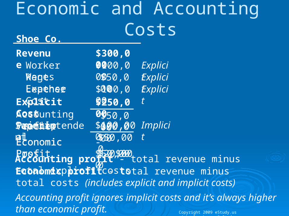
Economic and Accounting CostsShoe Co.Revenue $300,000
Explicit Cost $250,000Accounting ProfitTeacher $30,000
Economic Profit $20,000
Principal $50,000Superintendent $100,000$50,000
Worker Wages $100,000Rent Expense $50,000Leather Cost $100,000
ExplicitExplicitExplicit
$0Economic Profit - $50,000Economic Loss
Implicit
Accounting profit - total revenue minus total explicit costs
Accounting profit ignores implicit costs and it’s always higher than economic profit.
Economic profit - total revenue minus total costs (includes explicit and implicit costs)
Copyright 2009 eStudy.us [email protected]

Economic and Accounting Costs- a time period when at least one input is fixed
- A time period when all inputs are variable
― Factory― Special equipment― Land
Short Run
Long Runfirms can build more factories, or sell existing ones
Cost for a fixed input is termed Fixed Cost
In the long run, ATC at any Q is cost per unit using the most efficient mix of inputs for that Q (the factory size with the lowest ATC)

Role of Time in Cost Analysis• Incremental Cost
• Incremental cost is the change in cost tied to a managerial decision.
• Incremental cost can involve multiple units of output.
• Marginal cost involves a single unit of output.
• Sunk Cost• Irreversible expenses incurred previously.• Sunk costs are irrelevant to present decisions.

Short-run Cost Curves• Short-run Cost Categories
• Total Cost = Fixed Cost + Variable Cost• For averages, ATC = AFC + AVC• Marginal Cost, MC = ∂TC/∂Q
• Short-run Cost Relations• Short-run cost curves show minimum cost in a
given production environment.

Short-run Cost Curves
Copyright 2010 eStudy.us [email protected]
TFC
$10
- Fixed Cost (TFC)
Q
0123456789
$10
$10$10$10$10
$10$10$10$10
TVC
$0$4
$7$11$18$28
$47$74$112$162
TC
$10$14
$17$21$28$38
$57$84$122$172
MC
$4
$3$4$7$10
$19$27$38$50
- Variable Cost (TVC)
AFC
--$10.00
$5.00$3.33$2.50$2.00
$1.67$1.43$1.25$1.11
AVC
--$4.00
$3.50$3.67$4.50$5.60
$7.83$10.57$14.00$18.00
ATC
--$14.00
$8.50$7.00$7.00$7.60
$9.50$12.00$15.25$19.11
- Total Cost (TC)
costs that don’t vary as output changes costs that do vary as output changes TC = TFC + TVC
- Marginal Cost (MC) the cost of producing one more output (Q)
𝑀𝐶=∆𝑇𝐶∆𝑄
AFAVAT

Short-run Cost CurvesCalculation Equations
Copyright 2010 eStudy.us [email protected]
at Q = 6
𝐴𝐹𝐶=𝑇 𝐹𝐶𝑄
𝐴𝑉𝐶=𝑇 𝑉 𝐶𝑄
𝐴𝑇𝐶=𝑇 𝐶𝑄
𝐴𝑇𝐶=𝐴𝐹𝐶+𝐴𝑉𝐶
𝑀𝐶=∆𝑇𝐶∆𝑄
=𝑇𝐶1−𝑇𝐶0
𝑄1−𝑄0
$57−$386−5
=$191
=$19
$106
=$1.67
$ 476
=$ 7.83
$576
=$9.50
$9.50=$1.67+7.83
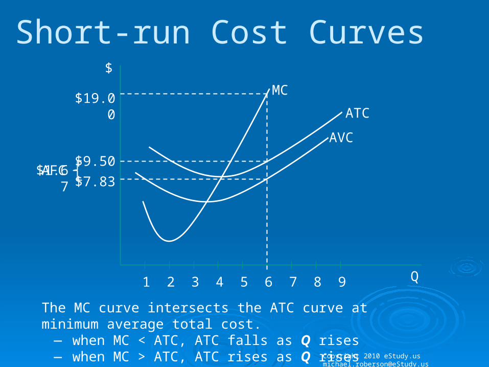
Short-run Cost Curves
Copyright 2010 eStudy.us [email protected]
MC
AVC
ATC
1 2 3 4 5 6 7 8 9
$9.50$7.83
$19.00
$1.67AFC
The MC curve intersects the ATC curve at minimum average total cost.
— when MC < ATC, ATC falls as Q rises— when MC > ATC, ATC rises as Q rises
$
Q

Short-run Cost Curves
Copyright 2010 eStudy.us [email protected]
$3.00
25
Minimum Marginal Cost corresponds to maximum Marginal Product
MC
10 25 50 65 75 80
$
Q
MP
1 2 3 4 5 6 Labor
Q / Labor
Suppose an accountant earns $75 / hour and her marginal productivity is:
Third hour 25Fourth hour 15Fifth hour 10Sixth hour 5
$75$75$75$75
MP wage
𝑀𝐶=∆𝑇𝐶∆𝑄
=𝑤𝑎𝑔𝑒𝑀𝑃 𝑙
¿$ 7525
=$3
$3$5$7.5$15
MC
$7.50
10

Long-run Cost Curves• Long-run total cost curves show minimum
total cost in an ideal environment.• Economies of Scale
• Increasing returns to scale imply falling average costs.
• Constant returns to scale implies constant average costs.
• Decreasing returns to scale implies rising average costs.

Long-run Cost Curves
$
Output
Long Run Average Cost
Short Run Average Cost
Economies to ScaleConstant Returns to Scale
Diseco
nomies to
Scale

Cost Elasticities Econ. of Scale• Cost elasticity measures the percentage
change in cost following a one percent change in output.
• Cost elasticity measures returns to scale.• EC < 1 means increasing returns (falling AC).
• EC = 1 means constant returns (constant AC).
• EC > 1 means decreasing returns (rising AC).

Long-run Cost Curves
$
Output
Long Run Average Cost
Min LRACLeast Cost Plant

Firm Size and Plant Size• Multi-plant Economies and Diseconomies of
Scale• Multi-plant economies are cost advantages from
operating several plants.• Multi-plant diseconomies are coordination costs from
operating several plants.
• Plant Size and Flexibility• Big plants can offer lower AC.• Smaller plants can make it easier to add and /or
subtract capacity.

Firm Size and Plant Size
$ $ $
Constant costs Declining costs U-shaped costs
𝑄∗ 𝑄𝐹 𝑄∗ 𝑄𝐹𝑄∗ 𝑄𝐹

Firm Size and Plant Size
𝑃=$ 940−$0.02𝑄𝑇𝑅=($ 940−$0.02𝑄 )𝑄=$940𝑄−$ 0.02𝑄2
𝑀𝑅=𝑑𝑇𝑅𝑑𝑄
=$940−$ 0.04𝑄
𝑀𝐶=𝑑𝑇𝐶𝑑𝑄
=$ 40+$0.02𝑄
𝑇𝐶=$250,000+$ 40𝑄+$ 0.01𝑄2

Firm Size and Plant Size𝑀𝑅=𝑀𝐶$940−$ 0.04𝑄=$40+$0.02𝑄
𝑃=$ 940−$0.02𝑄=$ 940−$0.02 (15,000 )=$640
𝜋=$940𝑄−$ 0.02𝑄2−($ 250,000+$40𝑄+$0.01𝑄2)
𝜋=−$ 0.03𝑄2+$900𝑄−$ 250,000𝜋=−$ 0.03 (15,000 )2+$900 (15,000)−$ 250,000
𝜋=$6,500,000

Firm Size and Plant Size
𝐴𝐶=𝑇𝐶𝑄
= $250,000+$ 40𝑄+$ 0.01𝑄2
𝑄
𝐴𝐶=$250,000𝑄− 1+$ 40+$ 0.01𝑄
𝑀𝐶=𝐴𝐶
$250,000𝑄− 1=$0.01𝑄
𝑄2=$ 250,0000.01
𝑄=√ $25,000,000=5,000

Firm Size and Plant Size
𝑀𝐶=$ 40+$ 0.02𝑄=$ 40+$ 0.02 (5,000 )=$140
Average cost is minimized at an output level of 5,000. This output level is the minimum efficient plant scale (MES). Because the average cost-minimizing output level of 5,000 is far less than the single plant profit maximizing activity level of 15,000 units, the profit maximizing level of total output occurs at a point of rising average costs. Thus a multi-plant alternative will reduce cost and increase profits.
𝑀𝐶=$ 40+$ 0.02𝑄=$ 40+$ 0.02 (15,000 )=$640
𝑀𝑅=$140=𝑀𝐶$940−$ 0.04𝑄=$140$0.04𝑄=$ 800𝑄=20,000

Firm Size and Plant Size
𝑂𝑝𝑖𝑚𝑎𝑙 𝑁𝑢𝑚𝑏𝑒𝑟 𝑜𝑓 𝑃𝑙𝑎𝑛𝑡𝑠=20,0005,000
=4
𝑃=$ 940−$0.02𝑄=$ 940−$0.02 (20,000 )=$540
𝜋=𝑇𝑅−𝑇𝐶𝜋=𝑃 ∙𝑄−4 ∙𝑇𝑜𝑡𝑎𝑙𝐶𝑜𝑠𝑡𝑝𝑒𝑟 𝑃𝑙𝑎𝑛𝑡𝜋=$540 (20,000 )−4 ($250,000+$ 40 (5,000 )+$ 0.01 (5000 )2)
𝜋=$8,000,000
𝑂𝑝𝑖𝑚𝑎𝑙 𝑁𝑢𝑚𝑏𝑒𝑟 𝑜𝑓 𝑃𝑙𝑎𝑛𝑡𝑠=𝑂𝑝𝑡𝑖𝑚𝑎𝑙𝑀𝑢𝑙𝑡𝑖𝑝𝑙𝑎𝑛𝑡 𝐴𝑐𝑡𝑖𝑣𝑖𝑡𝑦 𝐿𝑒𝑣𝑒𝑙𝑂𝑝𝑡𝑖𝑚𝑎𝑙 𝑃𝑟𝑜𝑑𝑢𝑐𝑡𝑖𝑜𝑛𝑃𝑒𝑟 𝑃𝑙𝑎𝑛𝑡

Economies of Scope• Economies of Scope Concept
• Scope economies are cost advantages that stem from producing multiple outputs.
• Big scope economies explain the popularity of multi-product firms.
• Without scope economies, firms specialize.
• Exploiting Scope Economies• Scope economics often shape competitive
strategy for new products.