Cosmology with the Large Synoptic Survey

Telescope: an Overview

Hu Zhan1 and J. Anthony Tyson2

1CAS Key Laboratory of Space Astronomy and Technology, National Astronomical

Observatories, A20 Datun Road, Chaoyang District, Beijing 100012, China2Department of Physics, University of California, One Shields Avenue, Davis, CA

95616, USA

E-mail: zhanhu@nao.cas.cn, tyson@physics.ucdavis.edu

Abstract. The Large Synoptic Survey Telescope (LSST) is a high etendue imaging

facility that is being constructed atop Cerro Pachon in Northern Chile. It is scheduled

to begin science operations in 2022. With an 8.4 m (6.5 m effective) aperture, a novel

three-mirror design achieving a seeing-limited 9.6 deg2 field of view, and a 3.2 Gigapixel

camera, the LSST has the deep-wide-fast imaging capability necessary to carry out an

18, 000 deg2 survey in six passbands (ugrizy) to a coadded depth of r ∼ 27.5 over 10

years using 90% of its observational time. The remaining 10% of time will be devoted

to considerably deeper and faster time-domain observations and smaller surveys. In

total, each patch of the sky in the main survey will receive 800 visits allocated across

the six passbands with 30 s exposure visits.

The huge volume of high-quality LSST data will provide a wide range of science

opportunities and, in particular, open a new era of precision cosmology with

unprecedented statistical power and tight control of systematic errors. In this review,

we give a brief account of the LSST cosmology program with an emphasis on dark

energy investigations. The LSST will address dark energy physics and cosmology in

general by exploiting diverse precision probes including large-scale structure, weak

lensing, type Ia supernovae, galaxy clusters, and strong lensing. Combined with

the cosmic microwave background data, these probes form interlocking tests on

the cosmological model and the nature of dark energy in the presence of various

systematics.

The LSST data products will be made available to the U.S. and Chilean scientific

communities and to international partners with no proprietary period. Close

collaborations with contemporaneous imaging and spectroscopy surveys observing at

a variety of wavelengths, resolutions, depths, and timescales will be a vital part of

the LSST science program, which will not only enhance specific studies but, more

importantly, also allow a more complete understanding of the universe through different

windows.

arX

iv:1

707.

0694

8v3

[as

tro-

ph.C

O]

9 M

ar 2

018

CONTENTS 2

Contents

1 Introduction 2

2 Cosmological Framework 5

2.1 Cosmic distances . . . . . . . . . . . . . . . . . . . . . . . . . . . . . . . 5

2.2 Growth of perturbations . . . . . . . . . . . . . . . . . . . . . . . . . . . 7

2.3 Two-point statistics of fluctuations . . . . . . . . . . . . . . . . . . . . . 8

3 Cosmic Frontiers 10

3.1 Accelerating universe . . . . . . . . . . . . . . . . . . . . . . . . . . . . . 10

3.2 Dark matter . . . . . . . . . . . . . . . . . . . . . . . . . . . . . . . . . . 13

3.3 Neutrino masses . . . . . . . . . . . . . . . . . . . . . . . . . . . . . . . . 15

3.4 Primordial perturbations . . . . . . . . . . . . . . . . . . . . . . . . . . . 17

4 Large Synoptic Survey Telescope 17

4.1 Telescope and camera . . . . . . . . . . . . . . . . . . . . . . . . . . . . . 18

4.2 Survey plan and performance . . . . . . . . . . . . . . . . . . . . . . . . 19

4.3 Data products . . . . . . . . . . . . . . . . . . . . . . . . . . . . . . . . . 21

4.4 Engaging the community . . . . . . . . . . . . . . . . . . . . . . . . . . . 22

5 LSST Probes of Cosmology 23

5.1 Large-scale structure (BAO) . . . . . . . . . . . . . . . . . . . . . . . . . 23

5.2 Weak gravitational lensing (WL) . . . . . . . . . . . . . . . . . . . . . . 26

5.3 Type Ia supernovae . . . . . . . . . . . . . . . . . . . . . . . . . . . . . . 30

5.4 Galaxy clusters . . . . . . . . . . . . . . . . . . . . . . . . . . . . . . . . 31

5.5 Strong lensing . . . . . . . . . . . . . . . . . . . . . . . . . . . . . . . . . 32

5.6 Joint analyses . . . . . . . . . . . . . . . . . . . . . . . . . . . . . . . . . 32

6 Summary 37

1. Introduction

Breakthrough discoveries have greatly expanded the boundary of our perceptible

universe from the solar system to the Milky Way, to the Realm of the Nebulae [1],

and to the afterglow of the Big Bang [2]. Tantalizing evidence for new physics from

our cosmic quest calls for a new generation of powerful survey facilities. Indeed, not

only do astronomers fully endorse research on the physics of the universe with long-term

planning exercises such as Cosmic Vision [3] — the European Space Agency’s science

program for 2015-2025 and New Worlds, New Horizons in Astronomy and Astrophysics

[4] — the 2010 US Decadal Survey of Astronomy and Astrophysics (Astro2010), but

physicists also fully recognize the potential to advance our fundamental understanding

of the particle world through its connection with the cosmos [5, 6]. What is truly

CONTENTS 3

exciting is that, after more than a decade of community efforts, ambitious projects like

the Large Synoptic Survey Telescope‡ (LSST) are now on track for operations starting

in the early 2020s.

It was realized through early dark matter mapping experiments in the 1980s

and 1990s [e.g., 7–11] that a huge survey volume was ultimately needed for useful

cosmological tests with imaging surveys. Specifically, the survey should be both deep

and wide. This enables precision cosmology by boosting the sample size for methods

based on properties of individual objects, by suppressing the sample variance error and

shot noise for methods relying on spatial statistics of the objects, and by providing

information about the evolution of the universe. To complete such a survey in a

reasonable time, one must resort to a facility with high etendue or “throughput”, which

may be quantified by the product of the light-collecting area and the field of view (FoV)

in solid angle. It would be ideally a large-aperture wide-field telescope that delivers

superb image quality, which brings considerable challenges to both the optics and the

camera.

The need for a high-throughput instrument for dark matter mapping motivated

the Big Throughput Camera (BTC, community access started in 1996) [12, 13]. It

was hosted by the National Optical Astronomy Observatory (NOAO) at the 4-meter

telescope (later named Blanco telescope) at Cerro Tololo Inter-American Observatory.

The BTC on the Blanco telescope had the most powerful sky survey capability at that

time. The pixels critically sampled the sub-arcsecond seeing, and shift-and-stare imaging

provided very deep images over moderately wide FoV. Two groups of astronomers used

the BTC to search for type Ia supernovae (SNe Ia), trying to measure the expected

“deceleration” of the expansion of the universe. What they found was remarkable

[14, 15]: instead of decelerating, the universe is accelerating!

While the BTC could survey to r ∼ 26 over a few square degrees in a week, another

facility using a larger mosaic of the same 2K×2K pixel CCDs, but on a much smaller

telescope, was optimized for moderate depth, very wide field observations: the Sloan

Digital Sky Survey (SDSS, science operations started in 2000) [16]. The first phase of

the SDSS completed in 2005, and its imaging covered 8000 deg2 of the sky in 5 bands to

a depth of r ≤ 22.2 [17]. The SDSS has been hugely successful, broadly impacting not

only astronomy but also the way research in astronomy is done. With three extensions,

it has now gone well beyond its original goals.

A natural question was then whether we could meet the challenges of surveying

much deeper and, at the same time, significantly wider than the SDSS. An affirmative

answer in the late 1990s would seem optimistic, but progress has been made by

precursors such as the Deep Lens Survey [18], the Canada-France-Hawaii Telescope

Legacy Survey [19], the Panoramic Survey Telescope and Rapid Response System (Pan-

STARRS) [20], and the Dark Energy Survey [21]. With a sufficiently large etendue

one would not have to make choices between wide-shallow or deep-narrow surveys;

‡ http://www.lsst.org/

CONTENTS 4

one could have a facility that would do the best of both: deep and wide. Moreover,

with a large telescope the exposures could be short, enabling a deep-wide-fast survey

which could provide the data needed by a broad range of science programs from a

single comprehensive set of observations. Thus was born the idea of the “Dark Matter

Telescope” [22].

Plans for the wide-field Dark Matter Telescope and its camera were presented at

a workshop on gravity at SLAC National Accelerator Laboratory in August 1998 [23].

The science case for such a telescope was submitted to the 2000 US Decadal Survey of

Astronomy and Astrophysics (Astro2000) [24] in June 1999. This proposal emphasized

the broad science reach from cosmology to the time domain through data mining of

a single deep-wide-fast sky survey. Astro2000 recommended it highly as a facility to

discover near-Earth asteroids as well as to study dark matter and renamed it Large-

aperture Synoptic Survey Telescope (the word “aperture” is now omitted). Soon after,

a summer workshop on wide field astronomy was organized at the Aspen Center for

Physics in July 2001. This was the beginning of wide involvement by the scientific

community in the LSST. In 2002 NOAO set up a national committee to develop the

LSST design reference mission [25]. Meanwhile, plans for a multi-gigapixel focal plane

and initial designs for the telescope-camera-data system were being developed [26–28].

In 2002 the National Science Foundation (NSF) funded research and development

of the new CCDs required for the LSST, supplementing an investment already made by

Bell Labs. L. Seppala modified R. Angel’s original three-mirror optical design for the

telescope [29], creating a 10 deg2, very low distortion FoV. The LSST Corporation was

formed in 2002 to manage the project. An R&D proposal was submitted to the NSF

in early 2007 and favorably reviewed later that year. Thanks to a gift from C. Simonyi

and B. Gates, the LSST 8.4-m primary-tertiary mirror was cast in 2008, and in early

2009 the secondary mirror blank was cast as well.

A grass-roots effort in 2008 and 2009 by the astronomy community resulted in the

LSST Science Book [30], a 596 page compendium of breakthrough science applications

co-authored by 245 scientists. In addition, the community wrote many white papers on

LSST science applications as input to the Astro2010 decadal survey process. The effort

was well received, and the LSST was ranked by Astro2010 as the highest priority for

ground-based astronomy [4]. In February 2011 a construction proposal was submitted

to the NSF. After many project reviews, the NSF National Science Board gave approval

to begin LSST construction in August 2014. The LSST construction is on schedule, and

first light for engineering tests with a commissioning camera is scheduled for 2019, with

the decade-long main survey beginning in 2022.

With its high etendue and image quality, the LSST is naturally a powerful facility

for dark energy studies, and it will take advantage of multiple probes such as weak

lensing (WL), large-scale structure (LSS), SNe Ia, galaxy clusters, and strong lensing.

It is therefore classified as a Stage IV dark energy experiment, i.e., a next generation

project, by the Dark Energy Task Force (DETF) [31]. These same survey data also

enable related investigations such as the dark matter distribution on a variety of scales

CONTENTS 5

from galaxies to the LSS and the sum of neutrino masses.

The rest of the paper is arranged as follows. Section 2 and section 3 introduce,

respectively, a set of frequently encountered concepts in cosmology and several research

areas that are expected to advance significantly with the LSST. We give a concise

description of the LSST project in section 4 and discuss in section 5 the cosmological

probes that have been developed extensively within LSST Science Collaborations.

Although an emphasis is given to applications for dark energy studies, readers are

reminded that these probes are sensitive to other elements of cosmology as well. For

more thorough discussions of the LSST — its design, capabilities, and wide range of

science opportunities, see [30]; a shorter overview is also available on the arXiv [32]. A

detailed plan of the dark energy program for the LSST can be found in the white paper

of the LSST Dark Energy Science Collaboration (DESC) [33].

2. Cosmological Framework

Modern cosmology has established a successful framework that enables precision

interpretation of observational data. Such a framework is built upon Einstein’s General

Relativity (GR) and the profound principle that the universe must be homogeneous

and isotropic on sufficiently large scales. Clearly, alternative theories of cosmology may

be constructed by modifying either GR or the cosmological principle, which are indeed

areas of active studies. Nevertheless, GR plus the cosmological principle remains the

most effective and self-consistent theory to date that describes the universe from its

very early stage to the present. This section is hence focused on key elements of the

conventional cosmological framework.

2.1. Cosmic distances

The Friedmann-Lemaıtre-Robertson-Walker (FLRW) metric [34–37] is essential for

cosmology under the principle of spatial homogeneity and isotropy. The line element of

the FLRW metric is given by

ds2 = −c2dt2 + a2(t)

(dr2

1−Kr2+ r2dΩ

), (1)

where a(t) and K are the scale factor and the curvature of the universe, respectively.

For convenience, the scale factor a(t) is set to unity at present time t0. The FLRW

metric is independent of GR. The influence of gravity is through the dynamics, e.g., the

evolution of a(t), so quantities and relations derived solely from the FLRW metric are

often applicable to models of alternative gravity theories.

It is useful to define a distance that depends on the spatial coordinates only:

dD2C =

dr2

1−Kr2+ r2dΩ. (2)

Since the distance DC between two bodies at rest locally in the expanding universe does

not change with time, it is given the name “comoving distance.” For a photon heading

CONTENTS 6

toward the observer (ds = dΩ = 0), the radial comoving distance along its geodesic is

DC[r(t)] =

∫ r

0

dr′√1−Kr′2

=

∫ t0

t

cdt′

a(t′). (3)

With (3), one can link the observed redshift z of spectral lines of a distant object to

the scale factor a at the time of emission via 1 + z = a−1 [35]. The comoving distance

between the observer and the object at z can then be written as

DC(z) =

∫ z

0

cdz′

H(z′), (4)

where the Hubble parameter H[z(t)] ≡ a/a is a measure of the expansion rate of the

universe at z (or t), and the over-dot on a denotes derivative with respect to t. For two

objects along the line of sight at z1 and z2 (z2 > z1), respectively, the comoving distance

between them DC(z1, z2) equals DC(z2)−DC(z1). For completeness, the time since Big

Bang is given by

t(z) =

∫ ∞

z

dz′

(1 + z′)H(z′). (5)

Two practical definitions of distances are frequently used on cosmic scales: the

angular diameter distance dA and the luminosity distance dL. The former is the distance

that converts the angular size θ of an object into its linear size l perpendicular to the

line of sight, i.e., l ' dAθ (|θ| 1). The luminosity distance is the radius of the sphere

at which an isotropic light source with luminosity L would produce the observed flux F ,

i.e., L = 4πd2LF . By setting dt = dr = 0 in (1), one can see that ar is just the angular

diameter distance of the coordinate r as viewed from the origin. The integral over r in

(3) can be carried out to get

r ≡ SK(DC) =

K−1/2 sin[K1/2DC(z)

]K > 0

DC(z) K = 0

(−K)−1/2 sinh[(−K)1/2DC(z)

]K < 0

, (6)

so that

DA(z) ≡ (1 + z)dA(z) = SK [DC(z)] , (7)

where DA(z) is the comoving angular diameter distance. In lensing studies, one often

needs to calculate the angular diameter distance of an object at z2 as viewed by an

observer at z1 (z2 > z1):

DA(z1, z2) ≡ (1 + z2)dA(z1, z2) = SK [DC(z1, z2)] . (8)

The luminosity distance and the angular diameter distance satisfy the reciprocity

relation [38] (also known as the distance-duality relation), i.e., dL(z) = (1 + z)2dA(z).

It is valid as long as [e.g., 39, 40]: (1) space-time is described by a metric theory, (2)

photon geodesics are unique, and (3) photons are neither created nor destroyed along

the geodesics. The reciprocity relation is therefore independent of the FLRW metric or

GR, and it offers a fairly model independent test of cosmology.

CONTENTS 7

2.2. Growth of perturbations

Gravity drives the evolution of the universe. Hence, we put GR into context here. From

Einstein’s field equations one can derive the Friedmann equations(a

a

)2

=8πG

3(ρm + ρde)−

Kc2

a2(9)

a

a= −4πG

3[ρm + ρde(1 + 3wde)] , (10)

where G is the gravitational constant, ρm is the matter density§, ρde is the dark energy

density, wde is the dark energy equation of state (EoS), and we have neglected the

radiation component as well as the pressure of matter. Equation (10) shows that

wde < −1/3 is a necessary (but not sufficient) condition for dark energy to drive the

cosmic acceleration (a > 0). Conservation of energy leads to a generic scaling

ρx(z) = ρx(0) exp

[3

∫ z

0

1 + wx(z′)

1 + z′dz′], (11)

where the subscript x can be “m” or “de.” Since the EoS of matter wm is practically

zero in the redshift range directly observed by the LSST, we can drop the subscript “de”

in wde without confusion. Equation (9) can now be rewritten as

H2(z)

H20

= Ωm(1 + z)3 + Ωk(1 + z)2 + Ωde exp

[3

∫ z

0

1 + w(z′)

1 + z′dz′], (12)

where H0 ≡ H(0) is the Hubble constant, Ωm ≡ ρm(0)/ρc with ρc ≡ 3H20/(8πG),

Ωk ≡ −Kc2/H20 , and Ωde ≡ ρde(0)/ρc = 1 − Ωm − Ωk. If dark energy is just the

cosmological constant Λ (w = −1), ρde indeed will be a constant over time. A flat

universe dominated by the cosmological constant and cold dark matter (CDM) is often

referred to as the ΛCDM universe, and we use wCDM to denote the case w 6= −1.

Equation (12) shows that H0, Ωm, Ωde (or Ωk), and w(z) completely specify the

cosmic expansion history, which, in turn, determines the distances and time defined

in section 2.1.

Gravitational instability turns minute initial fluctuations into structures we observe

today. The growth history of these fluctuations provides crucial cross-checks of the

cosmological model. On linear scales, the overdensity of the perturbed density field

ρm(x, t) can be decomposed into a spatial component and a time component

δm(x, t) ≡ ρm(x, t)− ρm(t)

ρm(t)= δm(x)G(t), (13)

where G(t) is the linear growth function. Assuming that dark energy does not cluster

on scales of interest, one obtains for the fluctuations in matter

G+ 2HG = 4πGρmG. (14)

It can be seen that the Hubble expansion in (14) works against gravity, so the cosmic

acceleration slows down the growth of structures. Gravity in general affects both the

§ Including both ordinary matter and dark matter. The former is often referred to as baryons in

astronomy for convenience.

CONTENTS 8

Hubble expansion and the right-hand side of (14). Therefore, one can potentially

distinguish dark energy from modified gravity theories by examining both the expansion

history (or distances) and the growth history of the universe [e.g., 41–43] if dark energy

is completely homogeneous and isotropic.

In analyses of galaxy redshift surveys, one often needs the logarithmic growth rate

f(z) =d lnG

d ln a≈ [Ωm(z)]γ , (15)

where the growth index γ ∼ 0.55–0.6 is not overly sensitive to cosmological parameters

within the GR framework [44–47].

2.3. Two-point statistics of fluctuations

Statistics of the cosmic density field are crucial probes of the universe. In the linear

regime, the cosmic density field can be approximated by a Gaussian random field, whose

properties are all captured in its two-point statistics, i.e., the correlation function in

configuration space or, equivalently, the power spectrum in Fourier space. For this

reason, we discuss only the two-point statistics here. For higher-order statistics and

their applications, see, e.g., [48–50].

The correlation function of the overdensity δ(x) is defined as

ξ(∆x) = 〈δ(x)δ(x′)〉, (16)

where 〈. . .〉 denotes an ensemble average, and, because of isotropy, the correlation

function depends only on the separation ∆x = |x′ − x| between two points. Under the

assumption of homogeneity and ergodicity, one can conveniently replace the ensemble

average in (16) with a volume average. Real observations are made on the past light-

cone, not on a snapshot (i.e., a constant-time hypersurface) of the universe, so the

volume average of the light-cone differs slightly from that of the snapshot, which is seen

in N -body simulations [51, 52]. Such an effect is deterministic and can be precisely

calibrated.

The distribution of galaxies may differ from that of matter. A clustering bias is

thus introduced to account for the difference between the galaxy correlation function ξg

and the matter correlation function, i.e., ξg = b2ξ. The galaxy bias evolves with time

and depends on the halo mass [53–56]. It also varies with the scale but changes rather

slowly above tens of h−1Mpc [e.g., 57, 58]. While the galaxy bias is a complex subject

of research [see 59–62, for early theoretical investigations], we treat it as a constant for

simplicity. In analyses of galaxy clustering data, it is useful to model the galaxy bias in

detail, so that one can extract cosmological information from small scales [63–65].

The correlation of the Fourier modes δ(k) defines the power spectrum P (k)

〈δ(k)δ∗(k′)〉 = (2π)3δD(k − k′)P (k), (17)

where δD(k−k′) is the Dirac delta function. The power spectrum is often expressed in a

dimensionless form ∆2(k) = k3P (k)/2π2, which is roughly the amplitude of fluctuations

CONTENTS 9

in the logarithmic interval around k. By Fourier expanding δ(x) in (16), one finds that

the correlation function in configuration space is just the Fourier transform of P (k), i.e.,

ξ(∆x) =1

(2π)3

∫eik·xP (k)d3k. (18)

Real surveys have finite volume and resolution, so one applies the discrete Fourier

transform in practice. Since the power spectrum and the correlation function are

equivalent, data analyses can be performed with either statistic. Still, the complexity

of the analyses depends on both the adopted statistic and the application. Besides the

multiplicative galaxy bias, the galaxy power spectrum receives an additive term due to

the shot noise

Pg(k) = b2P (k) + n−1g , (19)

where ng is the galaxy number density. The galaxy bias in (19) is equivalent to that in

the galaxy correlation function if it is scale-independent.

The statistical error of the power spectrum at the wavevector k equals the power

spectrum itself, i.e., σPg(k) = Pg(k) [66]. The errors at different wavevectors are

independent under a Gaussian approximation, so the uncertainty of a band power can

be reduced effectively

σPg(k) =

√2

Nk

Pg(k), (20)

where Nk is the number of modes within a band of width ∆k. For a survey of volume

V , Nk ' k2∆kV/2π2. The uncorrelated errors make the power spectrum convenient for

at least theoretical studies. With observational effects and nonlinearity, one can still

decorrelate the modes with some effort [67, 68].

In the linear regime, where ∆2(k) 1, all the modes grow at the same rate with

no coupling to each other. Therefore, the linear power spectrum at a redshift well below

the redshift of the cosmic microwave background (CMB, z ∼ 1100) can be scaled from

that at a reference redshift (e.g., z = 0) using the linear growth factor

PL(k, z) =G2(z)

G2(0)PL(k, 0). (21)

Because of the complex nature of the galaxy bias, it is not straightforward to predict the

galaxy power spectrum precisely. One usually has to fit the galaxy bias parameter(s)

with data. However, it is encouraging that relatively simple bias models based on the

concept of halos [62, 69, 70] are largely consistent with current observations [71–74].

Perturbative calculations can extend the power spectrum prediction into the weakly

nonlinear regime [75–81]. Going further, one must resort to cosmological N -body

simulations. Tests with simulations have reached 1% level accuracy out to k ∼ 1hMpc−1

[82], which is within a factor of a few from the requirements of future surveys [83, 84].

However, the cost of running N -body simulations makes them impractical for direct

use in cosmological parameter estimation. A solution to this problem is in essence to

develop an advanced interpolation scheme that can quickly output the power spectrum

CONTENTS 10

with satisfactory accuracy from a minimum set of simulations spanning the parameter

space [85–88]. For less demanding applications, fitting formulae for the nonlinear matter

power spectrum [89–91] are convenient to use.

3. Cosmic Frontiers

Cosmology is a key science driver of the LSST. Although great discoveries often come

unexpected, there are many areas for which one can predict substantial progress with

the LSST. Here we give a brief account of several such areas.

3.1. Accelerating universe

The cosmic acceleration is undoubtedly a profound challenge to our understanding of

the universe [5, 6, 31]. So far investigations have been focused on two classes of models:

dark energy and modified gravity [for recent reviews, see 92–94]. The former is developed

under the framework in section 2 as a special component of the universe, while the latter

induces the acceleration with a new form of gravity. There are also models that admit

no new components or physics but attribute the acceleration to a breakdown of the

cosmological principle or an oversimplification of GR effects in the real universe [e.g.,

95–97]. These models are less popular, but they do invite a closer inspection of the

cosmological framework and the evidence for the cosmic acceleration.

Consider SNe Ia as an example. One may fit their luminosity distances with a

Friedmann model in section 2.2, and the acceleration can be deduced from the resulting

model parameters. Because the result is obtained under a model that allows acceleration

in the first place, it is hard to draw a definitive conclusion before exhausting all other

possibilities. Alternatively, one can estimate the deceleration parameter — a kinematic

quantity

q = −a2

a2

a

a=

d lnH

d ln(1 + z)− 1 (22)

without referring to the dynamics [98, 99]. Studies along this line indeed show that

q < 0, i.e., a > 0, at low redshift [100–102]. Since a involves the second derivative with

respect to time, measurements of the cosmic time or age of the universe at a series of

redshifts would give the most direct evidence. However, such measurements are rather

challenging. For example, the redshift drift effect can map the evolution of the cosmic

expansion rate in theory [103, 104]. But even if one could monitor an object’s redshift

stably over decades to measure a ∼ 10−9 change in its redshift, peculiar velocities

and other uncertainties associated with the object itself could easily dominate over the

signal [105, 106]. A more practical example is to measure the cosmic expansion rate

from age differences of passively evolving galaxies [107]. This technique has achieved

typical precision of 5-14% on the Hubble parameter up to z ∼ 1 [108], though further

improvement is needed to quantify the acceleration precisely via (22).

CONTENTS 11

A negative deceleration parameter signifies acceleration in an FLRW universe.

If, however, the cosmological principle does not hold, then one cannot use a global

scale factor like that in the FLRW metric to describe the expansion of the universe.

Consequently, the deceleration parameter, if measurable at all, becomes a local quantity,

and a local acceleration does not necessarily mean a global acceleration of the universe.

This is the case for models which place the observers in an accelerating void [109–111],

which are however in tension with the data [112, 113]. In addition, nonlinear evolution

of small-scale inhomogeneities have been postulated to cause an apparent acceleration

on much larger scales [95, 114–117]. Although such an effect is found to be negligible

[118–120], the question about the validity of the FLRW metric for interpreting real

observations is highly relevant and deserves careful examination.

Applying the FLRW metric with GR, one finds that a smooth component with

strong negative pressure, i.e., dark energy, is needed to drive the accelerated expansion.

Its simplest form, the cosmological constant Λ, was invented by Einstein nearly a century

ago to keep the universe static. Decades before the SN Ia results in 1998, many had

already argued for a positive cosmological constant based on a range of observations

including the LSS, CMB, Hubble constant, and so on [121–125]. Even a time-varying

cosmological “constant” due to a scalar field was proposed by Peebles & Ratra in 1988

[126]. Depending on the behavior of the scalar field’s kinetic and potential terms, one

arrives at the quintessence model (−1 < w < 1) [127], the phantom model (w < −1)

[128], and the quintom model (w can cross −1 with the help of two fields) [129]. Many

more dark energy models have been discussed in the literature, and interested readers

are referred to [130] for a review.

Phenomenologically, dark energy is characterized by its present energy density as

a fraction of the critical density Ωde and its EoS w. A major task of dark energy

experiments is thus to measure Ωde and reconstruct w as a function of redshift for

model comparison. A widely used parametrization of the EoS is w = w0 + wa(1 − a)

[131, 132]. The reciprocal of the area of the w0-wa error ellipse was introduced as a figure

of merit by the DETF [31] to evaluate the performance of various surveys‖. To fully

utilize the capability of future surveys (so-called Stage IV dark energy experiments),

one should go beyond the w0-wa parametrization [133, 134].

Besides strong negative pressure, dark energy might also have a sound speed that is

sufficiently low to allow appreciable clustering on very large scales. The sound speed of

standard quintessence is equal to the speed of light, while models such as k -essence [135]

can produce a sound speed well below the speed of light over certain period of time [136].

The effect of dark energy clustering might be detected with CMB and galaxy surveys

on very large scales [137, 138].

Modified gravity offers another mechanism to drive the cosmic acceleration. There

are two well studied models: Dvali-Gabadadze-Porrati (DGP) gravity [139] and f(R)

gravity [140, 141]. In the DGP model, matter is confined in a 4-dimensional brane, while

‖ The report uses the 95% confidence limit, i.e., roughly 2σ in the Gaussian case, to define the error

ellipse, but studies afterward frequently use the 68.3% confidence limit (1σ) instead.

CONTENTS 12

gravity can leak into the fifth dimension above a transition scale rc, causing it to weaken

faster than expected in a 4-dimensional space-time. The f(R) model replaces the Ricci

scalar R in the GR gravitational action with a function f(R). A suitable choice of f(R)

could accelerate the cosmic expansion. Unfortunately, neither model appears viable.

On the one hand, DGP gravity is inconsistent with observations [142]. On the other

hand, f(R) gravity is constrained to be so close to GR that dark energy is still needed

to drive the acceleration [143]. Nonetheless, it is useful to see from a specific example

how to generate the accelerated expansion. Hence, we include a few equations of the

DGP model here. The Friedmann equation becomes [144]

H2 − ε crc

√H2 +

Kc2

a2=

8πG3ρm −

Kc2

a2, (23)

where ε = ±1. An acceleration in the DGP model is produced with ε = +1. The linear

growth function satisfies [145]

G+ 2HG = 4πG(

1 +1

3β

)ρmG, (24)

where

β = 1− 2Hrc

c

(1 +

H

3H2

). (25)

Comparing with the corresponding equations in GR, one sees that DGP gravity (and

modified gravity in general) affects the linear growth by altering both the expansion

background, i.e., H on the left-hand side of (24), and the effective strength of gravity

on the right-hand side.

Distinguishing dark energy from modified gravity is of particular interest, as the

physics behind them are fundamentally different. If dark energy only affects the

background expansion, then one may detect the signature of modified gravity from

inconsistency between the expansion history and the growth history. With more generic

(parametrizations of) dark energy and modified gravity models, the task is thought to

be impossible [146, 147], though it may still be feasible for dark energy models with no

coupling to matter [148].

Redshift evolution of the Hubble parameter, angular diameter distance, linear

growth function, and growth rate are shown in figure 1 for five cosmological models.

The parameters of the ΛCDM model adopt Planck 2015 results [149]. The wCDM1

and wCDM2 models differ from the ΛCDM model only in the dark energy EoS. It is

relatively easy to tune different models to match either the expansion or the growth

history, but not so easy to match both. For instance, whereas the wCDM1 model is

practically indistinguishable from the DGP2 model in terms of DA(z) and H(z), the

differences in G(z) and f(z) are conspicuous. Although the wCDM2 model coincides

with the ΛCDM model in G(z) and f(z), measurements of DA(z) and H(z) to better

than 1% at multiple redshifts below z ∼ 2 can tell them apart. A similar case occurs

between the DGP1 and the DGP2 models.

CONTENTS 13

1 3 5 7 9

1 + z

0.95

1.00

1.05

1.10

1.15

H(z)/

Hre

f(z)

1 3 5 7 9

1 + z

0.92

0.94

0.96

0.98

1.00

1.02

1.04

DA(z)/D

Are

f(z)

1 3 5 7 9

1 + z

0.1

0.2

0.3

0.4

0.5

0.6

0.7

0.8

G(z)

1 3 5 7 9

1 + z

0.3

0.4

0.5

0.6

0.7

0.8

0.9

1.0

f(z)

ΛCDM: Ωm = 0.309, ΩΛ = 0.691

wCDM1: w = -0.76wCDM2: w0 = -1.2, wa = 0.6DGP1: rc = 1.0 cH−1

0

DGP2: rc = 0.789 cH−10

Figure 1. Upper left panel: Hubble parameter of various models relative to that of the

ΛCDM model with Ωm = 0.309 (solid line). The models are wCDM1 with w = −0.8

(dashed line), wCDM2 with w0 = −1.2 and wa = 0.6 (dot-dashed line), DGP1 with

rc = cH−10 (circles), and DGP2 with rc = 0.789cH−1

0 (squares). All models are flat.

Upper right panel: same as the upper left panel but for the angular diameter distance.

Lower left panel: linear growth factor of all the models. Lower right panel: growth

rate of all the models.

Figure 1 clearly demonstrates the value of accurately mapping both the expansion

history and the growth history of the universe. The Hubble parameter and different

types of distances allow us to distinguish the ΛCDM model from dynamical dark energy

models, while the growth function and growth rate are useful for breaking the degeneracy

between modifications to gravity and the background expansion effect. Note that

spectroscopic surveys are needed to measure H(z) and f(z) from radial baryon acoustic

oscillations (BAOs) [150–154] and the redshift distortion effect [155–158], respectively.

Future imaging and spectroscopic surveys will be able to constrain the quantities in

figure 1 to the percent level in many redshift bins up to z . 3 [159–161], which is

sufficient to distinguish models with even smaller differences than those shown.

3.2. Dark matter

Dark matter is another major frontier of cosmology and particle physics and has a much

longer history of study than dark energy. The existence of dark matter is evidence

for physics beyond the standard model. Astrophysical evidence for the existence of

dark matter comes from many directions including, for example, dynamics of galaxy

clusters, galaxy rotation curves, X-ray emissions from galaxies and clusters, and WL

CONTENTS 14

mass mapping [162–167]. Formation of galaxies and substructures within them requires

dark matter, or at least the main component of it, to have a low velocity dispersion

(hence “cold”) in the early universe [168]. Out of the diverse topics in dark matter

research, we can only touch upon a few that are relevant to the LSST. Readers are

referred to [169, 170] for thorough reviews.

Optical observations are crucial to dark matter studies that probe its gravitational

effects. An important application is to determine the mean density parameter of dark

matter ωdm = Ωdmh2 (equivalent to ρdm; ditto matter density ωm and baryon density

ωb) or its fraction Ωdm in the total matter-energy budget of the universe. One can

estimate Ωdm in a number of ways. Distance measurements can constrain the total

matter fraction Ωm, which is the sum of Ωdm and Ωb (neglecting radiation and other

minor components), and then Ωdm can be obtained with a prior on Ωb, which might also

be deduced from the same survey data. Sensitivity of the abundance of massive halos

and its evolution to Ωm (in combination with the normalization of density fluctuations

σ8) provides another way to determine Ωdm [171]. One can also estimate Ωdm and Ωb

from the shape of the matter power spectrum. So far, analyses of the CMB power

spectra have obtained the most precise results on these parameters [149, 172]. Surveys

like the LSST will eventually achieve similar or greater statistical power than analyses of

the CMB do and will enable significant improvement over CMB-only results [173, 174].

The left panel of figure 2 illustrates the difference between two ΛCDM models with

ωdm = 0.119 [149] and ωdm = 0.137 (15% higher than the former), respectively. The

reduced Hubble constant takes the value of h = 0.677 for both models. The power

spectra are calculated using class [175]. Note that the shape of the matter power

spectrum depends on ωdm and ωb rather than Ωdm and Ωb and that the different values

of Ωm in the two models cause a slight mismatch between their linear growth functions.

The power spectra at z = 0 are normalized at k = 0.02 Mpc−1. The prominent turnover

feature around keq ' 0.016hMpc−1 is related to the epoch of matter-radiation equality

(aeq ' 2.8× 10−4). In the radiation era, i.e., a < aeq, perturbations within the horizon

were frozen. Smaller-scale perturbations entered the horizon earlier and experienced

more suppression. After matter became dominant, perturbations of all scales evolved

identically until nonlinearity or non-gravitational interactions became important. A

higher matter density means that the matter-radiation equality occurred at an earlier

time when the horizon was smaller. Therefore, the turnover scale shifts to a smaller

scale (larger k) with a higher ωdm if ωb remains the same. In terms of parameter

estimation, scales below the turnover generally provide stronger constraints. The wiggles

around k ∼ 0.1hMpc−1 in the power spectra are the BAO feature arising from the

perturbations in the same cosmic fluid that produced the CMB [176–178]. It is an

important cosmological probe as discussed in section 5.1.

The mean density of dark matter in the universe is only one piece of the puzzle.

More information is needed to decipher the physics of dark matter. Despite its success

on cosmological scales, the CDM paradigm is at odds with observations on galactic

and smaller scales, which have been phrased as the missing satellite problem (too many

CONTENTS 15

10−3 10−2 10−1 100

k (h Mpc−1)

102

103

104

P(k)

(h−3

Mpc

3)

z = 0

0.5P (k), z = 1

ωdm = 0.119, ωb = 0.022

ωdm = 0.137, ωb = 0.022

10−3 10−2 10−1 100

k (h Mpc−1)

102

103

104

P(k)

(h−3

Mpc

3)

∑mνe = 0.2eV

z = 0

0.5P (k), z = 1

ωm = 0.141, ωb = 0.022

Massless NeutrinosMassive Neutrinos

Figure 2. Left : Linear (thin lines) and nonlinear (thick lines) matter power spectra

of two ΛCDM models with ωdm = 0.119 (solid lines) and ωdm = 0.137 (dashed

lines). Right : Same as left, but the ωdm = 0.137 model is replaced by a model with

massive neutrinos (∑mνi = 0.2 eV). The two models share the same matter density

of ωm = 0.141.

subhalos in simulations than observed) [179, 180] and the cusp-core problem (halos’

central dark matter profile much shallower than predicted) [181–184]. There is also a

related “too big to fail” problem (mismatch between massive subhalos in Milky Way-

like simulations and the observed bright satellites of the Milky Way) [185]. Two routes

to resolve the issues have been pursued: one is to investigate baryonic processes, such

as star formation and energetic feedback, that may lead to the observed properties

of dark matter structures [186], and the other tries to match the observations by

replacing CDM with, for example, warm dark matter, self-interacting dark matter, or

nonthermally produced dark matter [187–189]. Both approaches need full development

to establish a sound connection between dark matter theories and observations, which

will be indispensable for proper interpretations of dark matter particle experiments as

well. Besides studies of galaxies and their satellites, the small-scale dark matter power

spectrum probed by quasar spectra (known as the Lyα forest) and the local dark matter

density measured from the stellar distribution and kinematics will also provide vital

information about the physics of dark matter [e.g., 190, 191]. In rare merging systems

such as the Bullet cluster [192], galaxies and dark matter may be separated from the

hot X-ray gas. Based on the separation, kinematics, and other information, one can

place a limit on the dark matter self-interaction cross-section [193, 194]. The LSST and

other facilities together will greatly expand the samples for dark matter studies and

bring more insights with precision measurements.

3.3. Neutrino masses

Unlike dark energy and dark matter, neutrinos are part of the standard model of

particle physics, but the non-vanishing mass of at least one neutrino species still

needs explanation. Astronomical observations are crucial for determining the sum of

CONTENTS 16

neutrino masses (∑mνi , sum over three families) [149, 172, 195, 196]. With neutrino

oscillation results, the individual neutrino masses can be determined up to an ambiguity

between the normal hierarchy (one species much heavier than the other two) and the

inverted hierarchy (one species much lighter than the other two) [e.g., 197]. If∑mνi is

constrained to less than 0.1 eV, then the inverted hierarchy would be disfavored [198].

An accuracy of better than 0.02 eV is needed at∑mνi = 0.06 eV to exclude the inverted

hierarchy at more than 95% confidence level [199].

The Planck limit on∑mνi with CMB, BAO, SN Ia, and H0 data is 0.23 eV (95%)

for a ΛCDM universe [149], which is somewhat sensitive to datasets combined as well as

model assumptions. A more recent analysis tightens the bound to an interesting regime

of ∼ 0.1 eV [200]. The results indicate that the neutrinos decoupled from other matter

before matter-radiation equality and became non-relativistic, i.e., matter-like, during

matter domination. In this scenario, the matter-radiation equality is slightly delayed

compared to that with massless neutrinos (assuming the same total matter density).

Perturbations entering the horizon before the transition thus have slightly less time to

grow, while those afterward are not affected. Well below their free-streaming scale, the

neutrinos do not contribute to overdensities, but they are still counted toward the mean

matter density. Therefore, small-scale density perturbations continue to be suppressed

after the neutrinos’ non-relativistic transition. The overall suppression of the matter

power spectrum relative to that with massless neutrinos reaches a constant factor of

approximately ∆P/P ' −8fν at k & 5hMpc−1 for fν . 0.07 [201], where fν is the

mean fraction of neutrinos in matter. The effect on intermediate scales requires detailed

calculations [e.g., 202].

The right panel of figure 2 compares the matter power spectra of the ΛCDM

models with massless and massive neutrinos, respectively. For∑mνi = 0.2 eV, the

non-relativistic transition would occur at anr = 7.5 × 10−3, corresponding to a scale

of knr = 4.5 × 10−3 hMpc−1. Figure 2 indeed shows that the matter power spectra at

k . knr are not affected by the neutrino masses. The shift of the turnover scale is barely

discernible, and the suppression of the power spectra on small scales is pronounced.

Nonlinear evolution appears to amplify the suppression effect of the neutrino masses.

However, the nonlinear matter power spectra are calculated using the fitting formula

from [90], which does not include massive neutrinos. Simulations are needed to obtain

more accurate results with massive neutrinos [203, 204], and care must be taken to

properly setup the initial conditions [205].

Besides the sum of neutrino masses, astronomical observations also have sensitivity

to the number of neutrino species Nν (or the effective number of radiation components

Neff). Forecasts with ideal assumptions predict that future surveys will reduce the

uncertainties to roughly 0.02 eV on∑mνi and 0.05 on Neff [198, 206, 207]. Therefore,

it is within the statistical capability of these surveys to determine the sum of neutrino

masses given the minimum possible value of∑mνi ∼ 0.06 eV and to positively detect

extra neutrino or radiation species. The challenge is to disentangle neutrino effects

from those of other astrophysical and observational factors such as the galaxy bias and

CONTENTS 17

systematics.

3.4. Primordial perturbations

Previous subsections have shown the importance of the density fluctuations for

determining the composition of the universe, though the origin of the fluctuations

remains to be addressed. A generic prediction of inflationary models is that quantum

fluctuations in the inflaton — a scalar field that drove inflation — seeded the density

fluctuations today [e.g., 208]. Inflaton perturbations were stretched outside the

horizon during inflation and reentered the horizon afterward as metric perturbations,

which became initial conditions of the density fluctuations. The primordial metric

perturbations are nearly scale invariant, so that the corresponding initial matter power

spectrum P (k) ∝ kns with the power spectral index ns ∼ 1. A small departure of

ns from unity is due to the slowly varying Hubble parameter and the inflaton field

during inflation. Besides the inflaton perturbations, gravitational waves generated

during inflation induce B-mode polarization in the CMB [209, 210], which have been

vigorously pursued by a number of experiments [211–213].

The primordial perturbations are of great interest for studies of inflation. Evolution

of the second-order perturbations after inflation always produces some amount of non-

Gaussianity, which is quantified by fNL — a coefficient of the second-order term in the

gravitational potential. A null detection at the level of fNL ∼ 1 would rule out the

standard cosmological model [e.g., 214]. As mentioned in section 3.2, physics within

the horizon has altered the perturbations that reentered the horizon before the matter-

radiation equality; only very large-scale modes are unaffected. Therefore surveys of huge

volumes are necessary to infer the primordial perturbation spectrum and to probe the

physics in the inflation era. CMB experiments have made remarkable achievements in

this area [e.g. 215, 216], though these results are based on a two-dimensional projection

of three-dimensional modes. The LSST and other surveys will enable studies of the

primordial perturbations with a comparable statistical power based on galaxy statistics

in a huge three-dimensional volume [173, 217].

4. Large Synoptic Survey Telescope

The LSST is a powerful facility for cosmological studies. It will have an 8.4 m (6.5 m

effective) primary mirror, a 9.6 deg2 FoV, and a 3.2 Gigapixel camera. An illustration

of the LSST Observatory is shown in figure 3. This system will have unprecedented

optical throughput and can image about 10,000 deg2 of sky in three clear nights using

30 s “visits” per each sky patch twice per night, with typical 5σ depth for point sources

of r ∼ 24.5 (AB magnitude). The detailed cadence will be decided by the Science

Advisory Committee via simulations of observing scenarios. The system is designed

to yield high image quality as well as superb astrometric and photometric accuracy.

The project is in the construction phase and will begin regular survey operations by

CONTENTS 18

Figure 3. The LSST Observatory: artist’s rendering of the dome enclosure with the

attached summit support building on Cerro Pachon in Northern Chile. The LSST

calibration telescope is shown on an adjacent rise to the right. Image credit: the LSST

Project/NSF/AURA.

2022. The survey area will be imaged multiple times in six bands, ugrizy, covering

the wavelength range 320–1050 nm. About 90% of the observing time will be devoted

to a deep-wide-fast survey mode which will uniformly observe an 18,000 deg2 region of

the southern sky over 800 times (summed over all six bands) during the anticipated

10 years of operations, and yield a co-added map to r ∼ 27.5. These data will result

in a relational database including 20 billion galaxies and a similar number of stars,

and will serve the majority of the primary science programs. The remaining 10% of

the observing time will be allocated to special projects such as a very deep and fast

time domain survey. The goal is to make LSST data products including the relational

database of about 30 trillion observations of 37 billion objects available to the public

and scientists around the world.

4.1. Telescope and camera

The large LSST etendue is achieved in a novel three-mirror design (modified Paul-Baker

Mersenne-Schmidt system) with a very fast f/1.2 beam [29]. The optical design has

been optimized to yield a large FoV, with seeing-limited image quality, across a wide

wavelength band. Incident light is collected by an annular primary mirror, having an

outer diameter of 8.4 m and inner diameter of 5 m, creating an effective filled aperture

of ∼ 6.5 m in diameter. The collected light is reflected to a 3.4 m convex secondary, then

onto a 5 m concave tertiary, and finally into the three refractive lenses of the camera.

In broad terms, the primary-secondary mirror pair acts as a beam condenser, while the

aspheric portions of the secondary and tertiary mirror act as a Schmidt camera. The

CONTENTS 19

-75°-60°-45°

-30°-15°

0°

15°30°

45°60° 75°

50 55 60 65 70 75Number of visits u band

-75°-60°-45°

-30°-15°

0°

15°30°

45°60° 75°

70 75 80 85 90 95 100 105 110Number of visits g band

-75°-60°-45°

-30°-15°

0°

15°30°

45°60° 75°

180 185 190 195 200 205 210 215 220Number of visits r band

-75°-60°-45°

-30°-15°

0°

15°30°

45°60° 75°

180 185 190 195 200 205 210 215 220Number of visits i band

-75°-60°-45°

-30°-15°

0°

15°30°

45°60° 75°

160 165 170 175 180 185 190 195 200Number of visits z band

-75°-60°-45°

-30°-15°

0°

15°30°

45°60° 75°

160 165 170 175 180 185 190 195 200Number of visits y band

Figure 4. The distribution of the 6 band visits on the sky for a simulated realization of

the baseline cadence. Image credit: Lynne Jones and the LSST Project/NSF/AURA.

3-element refractive optics of the camera correct for the chromatic aberrations induced

by the necessity of a thick Dewar window and flatten the focal surface. All three mirrors

will be actively supported to control wavefront distortions introduced by gravity and

environmental stresses on the telescope.

The LSST camera provides a 3.2 Gigapixel flat focal plane array, tiled by 189

4K×4K CCD sensors with 10µm pixels. This pixel count is a direct consequence of

sampling the 9.6 deg2 FoV (0.64 m diameter) with 0.2 arcsec× 0.2 arcsec pixels (Nyquist

sampling in the best expected seeing of ∼ 0.4 arcsec). The sensors are deep-depleted

high-resistivity silicon back-illuminated devices with a highly segmented architecture

that enables the entire array to be read in 2 seconds. The CCDs are grouped into 3×3

rafts, each containing its own dedicated electronics. The rafts are mounted on a silicon

carbide grid inside a vacuum cryostat, with an intricate thermal control system that

maintains the CCDs at an operating temperature of 173 K. The entrance window to

the cryostat is the third of the three refractive lenses in the camera. The other two

lenses are mounted in an optics structure at the front of the camera body, which also

contains a mechanical shutter, and a carousel assembly that holds five large optical

filters. The sixth optical filter can replace any of the five via a procedure accomplished

during daylight hours.

4.2. Survey plan and performance

The main deep-wide-fast survey (typical single visit depth of r ∼ 24.5) will use about

90% of the observing time. The remaining 10% of the observing time will be used to

obtain improved coverage of parameter space such as very deep observations. These

deeper fields (deep-drilling fields) will aid in statistical completeness studies for the

CONTENTS 20

Table 1. The LSST Baseline Design and Survey Parameters

Quantity Baseline Design Specification

Optical Config. 3-mirror modified Paul-Baker

Mount Config. Alt-azimuth

Final f-ratio, aperture f/1.234, 8.4 m

FoV, etendue 9.6 deg2, 319 m2deg2

Plate Scale 50.9µm/arcsec (0.2” pix)

Pixel count 3.2 Gigapix

Wavelength Coverage 320 – 1050 nm, ugrizy

Single visit depths, design a 23.9, 25.0, 24.7, 24.0, 23.3, 22.1

Mean number of visitsb 56, 80, 184, 184, 160, 160

Final (coadded) depthsc 26.1, 27.4, 27.5, 26.8, 26.1, 24.9

a Design specification from the Science Requirements Document (SRD) [220] for 5σ

depths for point sources in the ugrizy bands, respectively. The listed values are

expressed on AB magnitude scale, and correspond to point sources and fiducial zenith

observations (about 0.2 mag loss of depth is expected for realistic airmass distributions).b An illustration of the distribution of the number of visits as a function of bandpass,

taken from Table 24 in the SRD.c Idealized depth of coadded images, based on design specification for 5σ depth and the

number of visits in the penultimate row (taken from Table 24 in the SRD).

main survey, since they will likely have deep spectroscopy as well as infrared coverage

from other facilities. The observing strategy for the main survey will be optimized for

homogeneity of depth and number of visits. In times of good seeing and at low airmass,

preference will be given to r-band and i-band observations which are used in WL. The

visits to each field will be widely distributed in position angle on the sky and rotation

angle of the camera in order to minimize systematic effects on the point-spread function

(PSF), which could introduce shear systematics in faint galaxies. Simulations of LSST

operations use actual weather data from the Chilean site. The detailed cadence in time

and space across the sky is being optimized with these simulations. We show one such

simulation of the 6 band coverage in figure 4 [218, 219].

The universal cadence proposal excludes observations in a region of 1000 deg2

around the Galactic Center, where the high stellar density leads to a confusion limit at

much brighter magnitudes than those attained in the rest of the survey. The anticipated

total number of visits for a ten-year LSST survey is about 2.8 million. The per-band

allocation of these visits is shown in table 1. The adopted time allocation (see table 1)

includes a slight preference for the r and i bands because of their dominant role in

star/galaxy separation and WL measurements.

Precise determination of the PSF across each image, accurate photometric and

astrometric calibration, and continuous monitoring of system performance and observing

CONTENTS 21

conditions will be needed to reach the full potential of the LSST mission. The

dark energy science requires accurate photometric redshifts, so the LSST photometry

will be calibrated to unprecedented precision. Auxiliary instrumentation, including a

1.5 m calibration telescope, will provide the calibration parameters needed for image

processing, to calibrate the instrumental response of the LSST hardware [221], and to

measure the atmospheric optical depth as a function of wavelength along the LSST line

of sight [222].

4.3. Data products

The rapid cadence and length of the LSST observing program will produce

approximately 15 TB per night of raw imaging data. The large data volume, the time

domain aspects, and the complexity of processing involved makes it impractical to rely

on the end users for the data reduction. Instead, the data collected by the LSST system

will be automatically reduced to scientifically useful catalogs and images. Over the ten

years of LSST operations and 11 data releases, this processing will result in cumulative

processed data of about 500 PB for imaging, and over 50 PB for the catalog databases.

The final data release catalog database alone is expected to be approximately 15 PB in

size.

Data collected by the LSST telescope and camera will be automatically processed

to data products — catalogs, alerts, and reduced images. These products are designed

to enable a large majority of LSST science cases, without the need to work directly with

the raw pixels. We give a high-level overview of the LSST data products here; further

details may be found in the LSST Data Products Definition Document [223], which is

periodically updated. These data will be served via a relational database.

Two major categories of data products will be produced and delivered by the

LSST: Level 1 and Level 2. Level 1 are time domain: data products which support the

discovery, characterization, and rapid follow-up of time-dependent phenomena. Level 2

data products are most relevant to cosmology: they are designed to enable systematics-

and flux-limited science, and will be made available in annual Data Releases. These will

include the single-epoch images, deep coadds of the observed sky, catalogs of objects

detected in the LSST data, catalogs of sources (the detections and measurements of

objects on individual visits), and catalogs of “forced sources” – measurements of flux on

individual visits at locations where objects were detected by the LSST or other surveys.

LSST Level 2 processing will rely on multi-epoch model fitting, or MultiFit, to perform

near-optimal characterization of object properties. Although the coadded images will be

used to perform object detection, the measurement of their properties will be performed

by simultaneously fitting (PSF-convolved) models to single-epoch observations. An

extended source model — a constrained linear combination of two Sersic profiles — and

a point source model with proper motion — will generally be fitted to each detected

object.

For the extended source model fits, the LSST will characterize and store the shape of

CONTENTS 22

the associated likelihood surface (and the posterior) – not just the maximum likelihood

values and covariances. The characterization will be done by sampling, with up to ∼ 200

(independent) likelihood samples retained for each object. For reasons of storage cost,

these samples may be retained only for those bands of greatest interest for WL studies.

While a large majority of science cases will be adequately served by Level 1 and 2

data products, a limited number of highly specialized investigations may require custom,

user-driven, processing of LSST data. This processing will be most efficiently performed

at the LSST Archive Center, given the size of the LSST data set and the associated

storage and computational challenges. To enable such use cases, the LSST DM system

will devote the equivalent of 10% of its processing and storage capabilities to creation,

use, and federation of so-called “Level 3” (user-created) data products. It will also

allow the science teams to use the LSST database infrastructure to store and share

their results. The LSST Archive Center and U.S. data access center will be at the

National Center for Supercomputing Applications (NCSA) [224]. Users will access the

LSST data through a Data Access Center web portal, a Jupyter Notebook interface,

and machine accessible web application programming interfaces. The web portal will

provide data access and visualization services, and the Notebook interface will enable

more sophisticated data analysis.

4.4. Engaging the community

The LSST database and the associated object catalogs will be made available to the U.S.

and Chilean scientific communities and to international partners with no proprietary

period. The LSST project has been working with international partners to make LSST

data products available worldwide. User-friendly tools for data access and exploration

will be provided by the LSST data management system. This will support user-initiated

queries and will run on LSST computers at the archive facility and the data access

centers.

Because of the volume of the LSST data, statistical noise will reach unprecedented

low levels so that some investigations will be limited by systematics, although at a level

far below those of previous surveys. Thus, those investigations will require organized

teams working together to optimize science analyses. LSST science collaborations have

been established in core science areas. The LSST DESC includes members with interests

in dark energy and related topics in fundamental physics.

The LSST Project is actively seeking and implementing input by the LSST science

community. The LSST science collaborations in particular have helped develop the

LSST science case and continue to provide advice on how to optimize their science with

choices in cadence, software, and data systems. During the commissioning period, the

Science Collaborations will play a role in the system optimization. The LSST Science

Advisory Committee provides a formal dialogue with the science community. This

committee also deals with technical topics of interest to both the science community

and to the LSST Project, and shares responsibility for policy questions with the Project

CONTENTS 23

Science Team.

5. LSST Probes of Cosmology

With its deep-wide-fast multiband imaging survey, the LSST will enable multiple

probes simultaneously for cosmological studies. Here we discuss several probes that

have been studied extensively: WL, LSS (or BAO¶), SNe Ia, galaxy clusters, and

strong lensing. WL is considered the most powerful among these probes, and, at

same time, it also imposes the most stringent requirements on the project (the

telescope, data management, and operations) and beyond (e.g., analysis pipelines,

computing infrastructure, simulations, theories, and so on). Since dark energy, or

cosmic acceleration in general, has become a common science driver of almost every

large extragalactic survey, these probes are often associated with dark energy, even

though they are also sensitive to various elements of cosmology as can be inferred from

section 3.

It is worth emphasizing the strength of utilizing multiple probes of the same survey

as well as those of different surveys to address the fundamental questions about the

universe. These probes will not only form interlocking cross-checks but also provide

means of calibrating mutual systematics, which would be a common challenge for surveys

like the LSST. The combination of WL and BAO is a particularly effective probe which

breaks degeneracies and suppresses systematics.

We note that one probe can be analyzed using the methods of another probe. For

example, in addition to their mass function, galaxy clusters may be studied for the LSS

that they trace and their WL and strong lensing effects. Different statistics can also be

applied to the same observables of each probe. For brevity, we introduce below only the

most discussed method(s) and statistic(s) for each probe.

5.1. Large-scale structure (BAO)

Statistical analysis of the large-scale galaxy distribution is the main tool of LSS studies.

Although LSS based on imaging data alone does not place strong constraints on the

dark energy EoS, it is generally more sensitive than other LSST probes to cosmological

parameters that affect the shape of the underlying matter power spectrum. LSS is

a quite mature field with decades of studies (e.g., [44]), and its formulism can find

applications in WL as well.

The LSST “gold sample” is expected to contain at least 2.6 billion galaxies at

iAB ≤ 25.3 mag. The redshift distribution is expected to follow n(z) ∝ z2 exp(−3.2z)

with an integrated surface number density of more than 40 arcmin−2 [30, section 3.7].

Although it is advantageous to utilize the full posterior probability distribution of the

¶ Much of the cosmological constraining power of the LSS in the LSST photo-z galaxy sample is from

the BAOs in the galaxy angular power spectra, so we use LSS and BAO interchangeably for the LSST

unless it is necessary to make a distinction.

CONTENTS 24

photometric redshift (photo-z) of each galaxy [225–227], we assume for convenience

that a photo-z is assigned to each galaxy. The science requirement on the photo-z rms

error per galaxy is σz(z) ≤ σz0(1 + z) with σz0 = 0.05, and the goal is to achieve

σz(z) ∼ 0.02(1 + z). However, even with σz0 as small as 0.02, the line-of-sight clustering

information is still severely suppressed at k & 0.02hMpc−1 [173, 228]. Therefore, it is

more practical to focus on angular clustering of the galaxies between photo-z bins.

With the Limber approximation [229], the galaxy angular power spectrum Cij(`) is

given by

Cij(`) =2π2

c`3

∫ ∞

0

dz H(z)DA(z)Wi(z)Wj(z)∆2(k; z) + δKij

1

ni(26)

Wi(z) = b(z)ni(z)/ni, (27)

where i and j identify the photo-z bins, ` is the multipole number, k = `/DA, δKij is the

Kronecker delta function, b(z) is the linear galaxy clustering bias, ni(z) is the redshift

distribution of galaxies in bin i, and ni =∫ni(z)dz. The last term on the right-hand

side of (26) is the shot noise due to discrete sampling of the continuous density field

with galaxies. The covariance between the power spectra Cij(`) and Cmn(`) per angular

mode is given by

Cov [Cij(`), Cmn(`)] = Cim(`)Cjn(`) + Cin(`)Cjm(`), (28)

and the rms error of Cij(`) is approximately

σ[Cij(`)] =

[Cii(`)Cjj(`) + C2

ij(`)

fsky(2`+ 1)

]1/2

, (29)

where fsky is the fraction of sky covered by the survey, e.g., fsky = 0.44 for the LSST.

The scale dependence of the galaxy bias becomes more pronounced below tens of

h−1Mpc, so one has to limit the application of (26) to large scales, or model the bias

in detail [63–65], or determine the galaxy bias with higher-order statistics [230, 231].

Equation (26) is also inaccurate on very large scales because the Limber approximation

breaks down; if primordial non-Gaussianity is considered, the galaxy bias needs to be

replaced by an effective bias that scales roughly as k−2 on very large scales [232, 233].

As an example, we show several galaxy angular power spectra in figure 5. The

LSST gold sample is assigned to 30 bins from photo-z of 0.15 to 3.5 with the bin width

proportional to 1 + z in order to match the photo-z rms error. Five auto power spectra

in their respective bins are given in the left panel of figure 5. The power spectra are

truncated at the high-` end where nonlinear evolution starts to become important.

Details of the calculations including the photo-z treatment can be found in [174]. The

right panel of figure 5 shows four cross power spectra between the bin centered on

z = 1.66 and its neighbors, and the auto spectrum at z = 1.66 is included for reference.

The amplitude of the cross power spectrum is largely determined by the overlap between

the two bins in true redshift space, so it decreases rapidly with the bin separation

under the Gaussian photo-z model. This property can help calibrate the photo-z error

distribution [174, 234].

CONTENTS 25

Figure 5. Left panel: Galaxy angular auto power spectra in five redshift bins (shifted

for clarity). The central photo-z of each bin is as labeled. The gray area indicates the

statistical error (cosmic variance and shot noise) per multipole for the bin centered at

z = 1.66. Right panel: Cross power spectra between bin i centered at z = 1.66 and bin

j centered at z = 1.22 (4th neighbor, dotted line), 1.43 (2nd neighbor, dashed line),

1.92 (2nd neighbor, dash-dotted line), and 2.20 (4th neighbor, long-dash-dotted line).

The auto power spectrum at z = 1.66 is the same as that in the left panel. Figure

adapted from [30] with updated survey data model.

One can clearly identify the BAO wiggles in the galaxy angular power spectra in

figure 5 despite the projection of three-dimensional fluctuations onto the sphere. These

wiggles are an imprint of acoustic waves in the tightly coupled cosmic fluid before the

universe became sufficiently cool to form neutral hydrogen around z ' 1100. The

primary CMB temperature anisotropy is a snapshot of these acoustic waves at the

last scattering surface, which is characterized by the sound horizon rs ∼ 150 Mpc at

that time [176–178]. The BAO feature is mainly a function of the matter density

and the baryon density, and its scale is large enough to remain nearly unchanged

in comoving space since z ' 1100. Therefore, it can serve as a standard ruler to

measure angular diameter distances (and Hubble parameters as well if accurate redshifts

can be obtained) and to further constrain cosmological parameters [150–152, 235–237].

Recent spectroscopic BAO surveys have measured several distances up to z = 2.3 with

precision of a few percent [238–241]. The LSST gold sample will enable more distance

measurements at the percent level up to z = 3 with BAOs only [159].

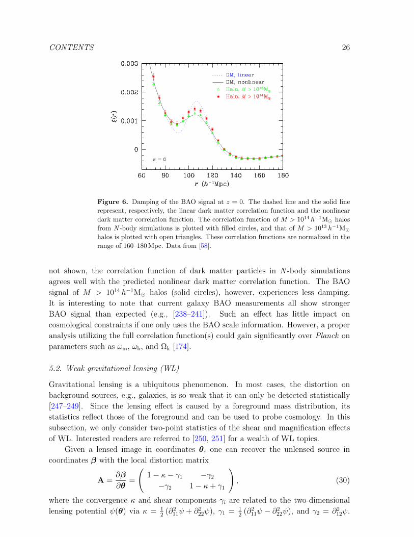
It is recognized that nonlinear evolution modifies the BAO feature over time by

damping its amplitude and shifting its scale by a fraction of a percent [242–245]. These

effects can be calibrated with simulations. Figure 6 demonstrates the damping effect on

the correlation functions at z = 0. The wiggles in the power spectrum become a peak

in the correlation function near rs ∼ 110h−1Mpc. The BAO signal in the nonlinear

dark matter correlation function (solid line, calculated with renormalized perturbation

theory [246]) has less contrast than that in the linear dark matter correlation function

(dotted line), and the shift of the BAO scale is not easily discernible. Although

CONTENTS 26

Figure 6. Damping of the BAO signal at z = 0. The dashed line and the solid line

represent, respectively, the linear dark matter correlation function and the nonlinear

dark matter correlation function. The correlation function of M > 1014 h−1M halos

from N -body simulations is plotted with filled circles, and that of M > 1013 h−1Mhalos is plotted with open triangles. These correlation functions are normalized in the

range of 160–180 Mpc. Data from [58].

not shown, the correlation function of dark matter particles in N -body simulations

agrees well with the predicted nonlinear dark matter correlation function. The BAO

signal of M > 1014 h−1M halos (solid circles), however, experiences less damping.

It is interesting to note that current galaxy BAO measurements all show stronger

BAO signal than expected (e.g., [238–241]). Such an effect has little impact on

cosmological constraints if one only uses the BAO scale information. However, a proper

analysis utilizing the full correlation function(s) could gain significantly over Planck on

parameters such as ωm, ωb, and Ωk [174].

5.2. Weak gravitational lensing (WL)

Gravitational lensing is a ubiquitous phenomenon. In most cases, the distortion on

background sources, e.g., galaxies, is so weak that it can only be detected statistically

[247–249]. Since the lensing effect is caused by a foreground mass distribution, its

statistics reflect those of the foreground and can be used to probe cosmology. In this

subsection, we only consider two-point statistics of the shear and magnification effects

of WL. Interested readers are referred to [250, 251] for a wealth of WL topics.

Given a lensed image in coordinates θ, one can recover the unlensed source in

coordinates β with the local distortion matrix

A =∂β

∂θ=

(1− κ− γ1 −γ2

−γ2 1− κ+ γ1

), (30)

where the convergence κ and shear components γi are related to the two-dimensional

lensing potential ψ(θ) via κ = 12

(∂211ψ + ∂2

22ψ), γ1 = 12

(∂211ψ − ∂2

22ψ), and γ2 = ∂212ψ.

CONTENTS 27

The convergence for a source at (θ, z) is a weighted integral of the overdensity along the

line of sight

κ(θ, z) =3H2

0 Ωm

2cDA(z)

∫ z

0

dz′DA(z′, z)DA(z′)

H(z′)δ(θ, z′)(1 + z′). (31)

The lensing magnification is given by µ = [(1− κ)2 − γ2]−1

. In the WL regime, |κ| and

|γ| are much smaller than unity, so that µ ' 1 + 2κ. For convenience, we use the word

“magnification” to also cover the case of demagnification.

Assuming that galaxies are randomly oriented in the absence of lensing, one can

estimate the shear from the average galaxy ellipticities within an area of appropriate

size. In practice, shear measurement is rather difficult, and it constitutes a major

source of systematic errors for WL. Much effort is being made to improve the accuracy

of shear measurement [e.g., 252–255]. Magnification changes the angular size of the

background in different directions while conserving the 4π solid angle as viewed by the

(freefall) observer. To be specific, let µ > 1 in a particular direction. On the one

hand, background galaxies are enlarged in this direction without altering their surface

brightness, so they appear brighter in terms of total flux. Since the apparent magnitude

is usually important for sample selection, faint galaxies that do not actually meet the

magnitude criterion could make the cut with the slight lensing boost. This effect would

increase the galaxy overdensity in the direction. On the other hand, magnification

also increases the angular separation between the background galaxies, reducing their

apparent surface density. These two competing effects do not cancel in general, and the

resulting galaxy number density fluctuations of the sample is another useful probe of

cosmology [256–259].

Angular power spectra (or two-point correlation functions) of shear signals are the

primary statistics of WL. They can be written in a similar form as (26)

Cγγij (`) =

2π2

c`3

∫ ∞

0

dz H(z)DA(z)W γi (z)W γ

j (z)∆2(k; z) + δKij

σ2γ

ni, (32)

W γi (z) =

3

2

ΩmH20

H(z)

DA(z)

a c

∫ ∞

z

dz′ni(z

′)

ni

DA(z, z′)

DA(z′), (33)

where σγ ∼ 0.2 is the rms shear of galaxies’ shape. The last term in (32) is known as the

shape noise, analogous to the shot noise in galaxy power spectra. The window function

W γi (z) is a broad function in redshift, peaking roughly midway between the sources and

the observer, so the cross power spectrum between two photo-z bins has an amplitude

close to that of the auto power spectrum in the lower photo-z bin.

It is customary to decompose the effects of shear systematics on the power spectrum

into multiplicative and additive components. The former arises from errors that are

correlated with the true shear signal, whereas the latter is uncorrelated with the signal.

The observed shear power spectra are then given by

Cγγij (`) = (1 + fi)(1 + fj)C

γγij (`) + Cadd

ij (`), (34)

where fi and fj account for the multiplicative errors, and Caddij (`) is the power spectrum

of the additive errors. In principle, these forms of errors also exist in the galaxy power

CONTENTS 28

spectra, but results from existing galaxy surveys suggest that they are sub-dominant.

For the LSST, the multiplicative errors of the shear power spectra need to be controlled

below 0.004 [260, 261], which is challenging. The dominant issue for ground-based

imaging is the PSF correction and its misestimation. This is particularly important for

tomographic cosmic shear where the evolution of the multiplicative correction to the

observed shear must correctly track the evolving size distribution of the source galaxies

with redshift. This low level of correction can be achieved for a deep tomographic WL

cosmic shear survey via simulations of the observations [262, 263]. For additive shear

it is not trivial to accurately determine the scale dependence of Caddij (`), but the level

of additive errors estimated from image simulations [264] suggests that it would not be

overly important for the LSST [265]. There are also small additive and multiplicative

PSF errors introduced by charge transport anomalies in the detector, however these

can be well calibrated and removed to first order in pixel processing. These errors,

particularly the multiplicative systematic, can be suppressed via observing strategy.

The amplitudes of these errors decrease rapidly in good image quality: this translates

to low airmass observing and a strategy of reimaging areas with previous poor seeing

exposures. Special dithering of exposures in subsequent re-visits to a field, in position

and camera angle, are planned.

The fact that WL measures directly the gravitational effect of all the matter and

that it is sensitive to both the expansion of the universe and the growth of cosmic

structures make it a powerful probe for the LSST, though it also has a number of

challenges besides shear estimation. A major source of error is uncertainties in the

photo-z error distribution or, equivalently, those in the true redshift distribution of

galaxies in each photo-z bin. Because the lensing kernel is very broad, a small error

in ni, e.g., a shift of its central redshift by ∆z ∼ 0.01, has practically no effect on

the shear power spectra. However, the cosmological interpretation would be sufficiently

different even with such a small redshift error that dark energy constraints would be

degraded considerably. It is recognized that the uncertainties in the mean and the width

of the true-redshift distribution of galaxies in each photo-z bin should not exceed a few

10−3(1 + z) for the LSST [174, 260, 266]. To achieve this goal, calibrations of both

individual galaxy redshift [267, 268] and the overall redshift distribution of the galaxies

in each photo-z bin are needed. The latter can be done to the required precision with

correlations between spatially overlapping photo-z and spectroscopic samples of brighter

galaxies over small patches of the survey area [269, 270]. Correlations between different

photo-z bins arising from incorrect assignment of the galaxies will also be helpful for the

calibration [174, 234, 271].

At the surface density of galaxies in the LSST gold sample, a small percentage will

be partially blended with other galaxies in the sample. This can cause outliers in photo-z

and generate about a 7% increase in WL shear noise unless addressed at the galaxy level

and statistically [272, 273]. If blends can be tagged (for example via a color gradient in

the combined core) then they may be eliminated from the sample. Conspicuous blends

with larger separation may be more easily identified, tagged and deblended.

CONTENTS 29

Another challenge for WL is intrinsic alignment [274, 275]. The orientation of

a galaxy can be influenced by the larger structure containing it, thus breaking the

assumption that galaxies orient randomly in the absence of lensing. The correlation of

galaxy orientations in the same structure would contaminate the true shear signal arising

from these galaxies’ common foreground mass distribution. Moreover, if these galaxies

themselves are taken as the foreground, then the structure they reside in would lens

galaxies in the background. The two effects of the same structure, intrinsic alignment

of the foreground galaxies and shear on the background galaxies, would correlate the

background and foreground galaxy orientations, contaminating the true correlation

between these galaxies’ shear signals. One needs to utilize photo-z information and

model the intrinsic alignment effects to minimize the impact on cosmology [276–279].

It is encouraging that marginalization of the intrinsic alignment systematics using a

simple phenomenological model may be sufficient for shear analyses [280, 281]. For the

LSST, faint blue galaxies will dominate its gold sample, and these are expected to be

less affected by intrinsic alignment [282].

Since magnification is extracted from the observed galaxy density fluctuations, it

avoids some of the difficulties with shear measurements but unfortunately inherits its

own systematics. The galaxy overdensity with magnification effect is approximately

[256, 283]

δg ' bδ + 5(s− 0.4)κ, (35)

where s = d logN/dm ∼ 0.2–0.6 is the logarithmic slope of the galaxy number counts at

the limiting magnitude m of the sample [e.g., 284]. The total angular power spectrum

of galaxies in photo-z bins i and j becomes [285]

C ggij = Cgg

ij + qiCκgij + qjC

gκij + qiqjC

κκij , (36)

where Cggij is the power spectrum due to galaxy intrinsic clustering, i.e., (26) with the

superscript g written out explicitly, qi = 5(si−0.4) with si for bin i, qiCκgij and qjC

gκij are

the galaxy-magnification cross power spectra, and qiqjCκκij is the magnification power

spectrum. Since the convergence for a lower redshift bin is uncorrelated with the galaxy

overdensity in a higher redshift bin, one of the cross terms vanishes for two well separated

bins. The galaxy-convergence power spectra Cκgij and Cgκ

ij and the convergence power

spectrum Cκκij can be calculated using (32) but with the two shear window functions

replaced by the galaxy window function (27) and the convergence window function,

which is identical to the shear window function (33).

The intrinsic clustering term is several orders of magnitude greater than the rest

in (36) when the photo-z bins i and j overlap significantly in true-redshift space; even

if they are well separated, the cross term Cgκij — assuming that bin j is at higher

redshift — still overwhelms Cκκij [286]. Furthermore, galaxies can be assigned to wrong

redshift bins because of photo-z errors, and the resulting spurious correlations can

be a serious contaminant for the magnification signal (conversely, magnification in

tomographic galaxy cross-correlations may be a contaminant for photo-z self-calibration

with the cross-correlations). Magnification systematic error can also arise from exposure

CONTENTS 30

depth spatial variations, dust, and blending of galaxy images [287]. Therefore, like the

case with shear, care must be taken when utilizing lensing magnification for precision

cosmology. As a cosmological constraint, magnification is subdominant to the other WL

probes.

5.3. Type Ia supernovae

SN Ia distances provided the most direct evidence for the accelerated cosmic expansion

[14, 15] and will remain an important dark energy probe in the future, though systematic

errors make it a less precise probe of cosmology by comparison to a joint analysis of

WL and BAO. The LSST is expected to obtain more than ten thousand well observed

SNe Ia (0.1 < z < 1.2) in the deep-drilling fields, hundreds of thousands reasonably-well

observed SNe Ia (z . 0.8) in the main survey, and millions of detection-only SNe Ia [30].

Such a huge sample of SNe Ia will enable new tests of cosmology such as the isotropy

of distance-redshift relation over the whole survey area.

The utility of SNe Ia for cosmology is based on their standardizable peak luminosity

that is tightly correlated with the initial decline rate of the light curve [288]. As such,

one can obtain the distance modulus, which is a function of cosmological parameters,

via [289–291]

µB = mB −MB + αx1 − βC (37)

where mB is the rest-frame B -band peak apparent magnitude, MB is the corresponding

absolute magnitude, x1 is the shape parameter of the light curve, C is the B − V color,

and α and β are nuisance parameters to be fitted along with MB (actually MB−5 log h)

and the cosmological parameters. Given the fairly low intrinsic dispersion of µB of

roughly 0.12, a single SN Ia can provide a luminosity distance with a nominal error of

6% (excluding the error in h). It is worth mentioning that SNe Ia are likely to be more

standard in the rest-frame near infrared [292, 293], though the LSST can observe only

up to 1.05µm.

The degeneracy between the Hubble constant and MB removes the absolute scale of

SN Ia distances and thus weakens their constraints on the cosmological parameters. The

remedy is to obtain a sample spanning as wide a redshift range as possible and to combine

a tight prior on the Hubble constant from external datasets. A number of technical

issues and systematic uncertainties could be the limiting factors for SN Ia cosmology

with next-generation surveys. Besides the challenges of obtaining very well sampled

light curves and precisely calibrated photometries, one also needs further investigation

on potential evolution of SN Ia properties over redshift, the relation between the SN Ia

peak luminosity and its host properties, and certainly the physics of SN Ia explosions.

The LSST survey, especially its deep-drilling fields, is tasked to address the technical

challenges for SN Ia cosmology, though effort is still being made to optimize the

operation strategy of the main survey. The huge LSST SN Ia sample can be divided

into many sub-samples for detailed studies of various systematics intrinsic to SNe Ia

themselves as well as biases arising from sample selection. Nonetheless, being an imaging

CONTENTS 31

survey, the LSST has its own challenges. For example, it has to correctly identify

SNe Ia and determine their redshifts based on photometric data only [294, 295]; even

though a small fraction of them will have spectroscopic follow-ups by other facilities,

the LSST still has to send out alerts promptly for the best candidates among millions

of transients every night with very high success-rate. It is also noted that photo-z errors

increase the apparent dispersion of the standardized SN Ia peak luminosity and that the

sample-averaged distance modulus–photo-z relation departs from the distance modulus–

true redshift relation [296]. One should account for these effects when estimating the

cosmological parameters.

5.4. Galaxy clusters

Galaxy clusters are the largest gravitationally bound systems in the universe. At the

high-mass end, a cluster may have thousands of member galaxies, while a low-mass

cluster can still contain many dozens of galaxies. Cluster cosmology is a rich topic and

involves observations from microwave to X-ray [for a review, see 297]. The primary

statistic of cluster cosmology for the LSST is the mass function, i.e., number density

of clusters as a function of mass at a certain redshift. Since clusters have grown under

gravitational instability from relatively high density regions of the fairly Gaussian initial

density fluctuations, one can roughly estimate the cluster mass function based on the

statistics of the Gaussian random field [298, 299]. For precision cosmology, more accurate

mass functions need to be extracted from N -body simulations [300, 301].

The cluster mass function is sensitive to both the geometry of the universe and the

growth of the large-scale structures, which makes it a powerful tool [302–304]. However,

the utility of clusters for precision cosmology critically depends on the knowledge of the

mass-observable relation and its scatter [305]. Because of the highly nonlinear process

of cluster formation and evolution, one has to rely on state-of-the-art simulations and

observations to precisely calibrate the mass-observable relation and its scatter for a

wide range of cosmology. It takes considerably more effort to properly include all the

relevant physics such as star formation and feedback in the simulations to reproduce

the observables [e.g., 306–308].

The LSST will produce a well observed sample of several hundred thousand clusters,

much larger than any previous surveys. It is not trivial to construct such a sample

efficiently from the LSST photometry data with high purity, high completeness, and

well understood selection function. Accurate photo-zs are needed for clusters as well.

Averaging over member galaxies’ redshifts generally reduces the photo-z errors, but

one has to be careful about any systematic redshift errors of the galaxy population in

the same cluster. Although WL measurements from the same LSST data can provide

important absolute cluster mass calibration, the scatter will be rather high (& 20%),

mainly due to triaxiality of the halos, projection effects along the line-of-sight, and

shape noise of shear measurements in the limited FoV [309]. It has been shown for Dark

Energy Survey (DES) that even a small fraction of the whole cluster sample (e.g., 200

CONTENTS 32

out of 105 expected) calibrated against a mass proxy of 10% scatter can enhance the

DES dark energy constraints by 50% [310]. As such, it is crucial to establish a tight

relation between cluster observables from LSST data with the cluster mass through

external low-scatter mass proxies, likely from X-ray observations [311].

5.5. Strong lensing

While WL effects are hardly discernible to the eye, background objects can be stretched

into arcs or even Einstein rings and be split into multiple images in the strong lensing

regime [e.g., 312–314]. A lens can be a galaxy or a galaxy cluster, and the background

sources are usually galaxies that are effectively static within the time span of an

observational program. In rare cases, one can find multiple-image systems of variable or

transient background sources such as active galactic nuclei (AGNs) and SNe [315, 316].

Different images of the same source means different paths and travel times for the

photons. The detailed configuration of the images and time delay between them are

determined by the mass distribution of the lens and the angular diameter distances

between the observer, the lens, and the source. Therefore, the strong-lensing time delay

can be a useful probe of cosmology. It is most sensitive to the Hubble constant [317] and

has recently been demonstrated to be able to constrain other cosmological parameters

such as the curvature parameter Ωk and the dark energy EoS parameter w [318, 319].

The typical time delay of a double lens (double-image system) is 1-3 months,

and much shorter delays of less than a day can occur when two images in a quad

lens (quadruple-image system) are very close to each other [320]. The LSST’s 10-year

rolling survey with 3-month seasons and a cadence of 5 days is suited for time delay

measurements of typical strong lensing systems. It is estimated that the LSST strong

lens sample will be at least an order of magnitude larger than previously obtained,

allowing time delays to be measured for more than 3000 strongly lensed quasars and

more than 100 strongly lensed SNe [320].

Like other LSST probes, strong-lensing time delay has its own challenges. Besides

lens monitoring and fitting for the time delay, one would also need accurate information

about the lens mass distribution and the source redshift. Moreover, the impact of

line-of-sight mass distribution on time delay needs to be taken into account, at least

statistically. In these areas, high-resolution observations from space, deep spectroscopy

on the ground, and modeling of the foreground structures will be particularly helpful for

strong-lensing cosmology with the LSST. In fact, with a major undertaking of external

follow-up observations, one can also probe the geometry of the universe with strongly

lensed sources in multiple source planes [321–323].

5.6. Joint analyses

The ability to produce large uniform data sets with high quality for multiple cosmological

probes is a crucial advantage of the LSST. These probes are affected by various

systematics and are sensitive to cosmology in different ways. Joint analyses of multiple

CONTENTS 33

probes not only improve parameter constraints but, more importantly, also enable

certain cross-calibrations of known systematics and detection of unknown systematics.

This allows one to perform robust tests on cosmological models and to explore with

confidence fundamental physics of the universe beyond current understanding.

The aforementioned probes are not always statistically independent. Correlations

arise when two probes are linked by common factors of real physical origin or

observational effects. For instance, WL shear of background galaxies is essentially

a function of the weighted projection of the line-of-sight mass distribution, which is

traced by galaxies. Thus, foreground galaxy density fluctuations are correlated with

the background shear, similar to the case of lensing magnification in section 5.2. This

effect is known as the galaxy-shear correlation or galaxy-galaxy lensing on large scales

(` . 1000) [63, 174, 324, 325], though, strictly speaking, the former can also include a

contribution from intrinsic alignment. The fact that WL and LSS (or BAO) techniques

share, at least partially, the same catalog of galaxies, and their photo-z systematics also

induces a correlation between the two probes. Such a correlation can be beneficial, as

the self-calibration of the photo-z error distribution by cross-bin galaxy power spectra

can reduce the sensitivity of the joint cosmological constraints of WL and BAO to

uncertainties in the photo-z error distribution [174, 234, 271]. Conversely, because of

the shared dark matter structure, the complementary WL and BAO measurements

break degeneracies in either probe.

Figure 7 demonstrates the synergy between WL and BAO based on Fisher matrix

analyses [67, 327, 328]. It is adapted from [326] with the survey area, galaxy redshift

distribution, and galaxy surface number density, respectively, adjusted to 18,000 deg2,

n(z) ∼ z2 exp(−z/0.3), and 40 arcmin−2. The number density is an effective value for

WL measurements, and the same is applied to BAO for convenience. The constraints of

the joint analysis are derived from the full set of galaxy-galaxy (i.e., galaxy clustering),

galaxy-shear (i.e., galaxy-galaxy lensing), and shear-shear power spectra. These power

spectra are affected by different powers of the galaxy bias and together can achieve

robust cosmological constraints in the presence of uncertainties in the galaxy bias

[63, 174]. Numerically, the galaxy-shear power spectra are equal to the galaxy-

convergence power spectra Cgκij in section 5.2. Planck CMB priors from a Fisher matrix

calculation in [174] are applied to all the results. While the constraints on the dark

energy EoS parameters, w0 and wa, from shear power spectra alone are sensitive to

systematic uncertainties in the photo-z error distribution, the joint results of shear

and galaxy power spectra remain fairly immune to these systematics. The dramatic

improvement of the joint results over the WL-only results is due to the mutual calibration

of the photo-z uncertainties as well as the uncertain factor of the galaxy bias. In other

words, much of the complementarity is in parameter space that has been marginalized

over. A demonstration of the constraining power of this joint analysis of cosmic shear,

galaxy-galaxy lensing and angular clustering has recently been obtained [329].

A forecast of cosmological constraints from combinations of three LSST probes and

real Planck data is given in figure 8. The Planck data consists of the joint likelihood of

CONTENTS 34

Figure 7. One-sigma error contours of the dark energy EoS parameters w0 and wafrom LSST WL shear power spectra alone (left panel) and shear and galaxy power

spectra analyzed jointly (right panel). The shaded areas represent the results with

statistical errors only. The solid contours correspond to those with the anticipated level

of systematic errors, which include the uncertainty in the photo-z error distribution

and additive and multiplicative errors in the power spectra. The assumed photo-

z systematics would require a redshift calibration sample of 3000 spectra per unit

redshift interval if the photo-z error distribution were Gaussian. This calibration can

be achieved statistically by using spectra of the brighter galaxies in the redshift interval

in small areas of the sky. The dotted contours relax the requirement to 188 spectra

per unit redshift. Figure adapted from [326] with updated survey data model.

the temperature-temperature (TT), temperature-E polarization (TE), E polarization-

E polarization (EE), and B polarization-B polarization power spectra in the range of

2 ≤ ` ≤ 29 and the foreground-marginalized joint likelihood of TT (30 ≤ ` ≤ 2508),

TE (30 ≤ ` ≤ 1996), and EE (30 ≤ ` ≤ 1996) band power spectra [330]. The CMB

power spectra are calculated using class with the lensing effect turned on [175]. The

LSST probes considered are WL, BAO, and SNe Ia. The set of cosmological parameters

includes w0, wa, ωm, ωb, Ωk, ns, H0, the redshift of reionization zrei, the helium fraction

YP, and the amplitude of the curvature power spectrum As. The sum of neutrino masses

is fixed at 0.06 eV.

The posterior probability distribution of the parameters are mapped with an affine

invariant Markov Chain Monte Carlo sampler [331, 332]. For LSST WL and BAO, we use

the corresponding Fisher matrices to calculate contributions to the final likelihood. The

Fisher matrices have been marginalized over non-cosmological parameters such as those

modeling the photo-z errors, galaxy biases, and errors in the power spectra. The fiducial

model of the Fisher matrices coincides with the Planck -only best-fit ΛCDM model [149],

and the fiducial values of the additional parameters, w0, wa, and Ωk, are set to −1, 0,

and 0, respectively. For LSST SNe Ia, a simple mock sample (tuples of distance modulus

and redshift) is generated under the fiducial cosmological model according to the yields

and redshift distributions from section 11.2 of [30]. The selection criterion is that each

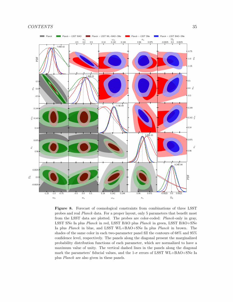
CONTENTS 35

PD

F

7.05E-02

1.86E-01

7.73E-04

3.49E-03

-0.0025 0.0 0.0025

Ωk

PD

F

9.24E-04

-0.5

0.0

0.5

wa

-0.5 0.0 0.5wa

0.14

0.142

0.144

ωm

0.14 0.142 0.144ωm

0.96

0.975

ns

0.96 0.975ns

-1.25 -1.0 -0.75

w0

-0.0025

0.0

0.0025

Ωk

-0.0025 0.0 0.0025Ωk

-1.25

-1.0

-0.75

w0

-0.5 0.0 0.5

wa

-0.5

0.0

0.5

wa

0.14 0.142 0.144

ωm

0.14

0.142

0.144

ωm

0.96 0.975

ns

0.96

0.975

ns

Planck Planck + LSST BAO Planck + LSST WL+BAO+SNe Planck + LSST SNe Planck + LSST BAO+SNe

Figure 8. Forecast of cosmological constraints from combinations of three LSST

probes and real Planck data. For a proper layout, only 5 parameters that benefit most

from the LSST data are plotted. The probes are color-coded: Planck -only in gray,

LSST SNe Ia plus Planck in red, LSST BAO plus Planck in green, LSST BAO+SNe

Ia plus Planck in blue, and LSST WL+BAO+SNe Ia plus Planck in brown. The

shades of the same color in each two-parameter panel fill the contours of 68% and 95%

confidence level, respectively. The panels along the diagonal present the marginalized

probability distribution functions of each parameter, which are normalized to have a

maximum value of unity. The vertical dashed lines in the panels along the diagonal

mark the parameters’ fiducial values, and the 1-σ errors of LSST WL+BAO+SNe Ia

plus Planck are also given in these panels.

CONTENTS 36

SN must be observed in three or more filters at a minimum signal-to-noise ratio of 20,

which results in roughly 400,000 SNe from the main survey and 12,000 SNe from the

deep-drilling survey in 10 years. While the deep-drilling survey can be optimized for SN

observations, it is impossible for the main survey to mass-produce SN light curves with

the same quality as can be achieved by the former. To be conservative, we reduce the

number of SNe Ia in the main sample somewhat arbitrarily to 100,000. The intrinsic

dispersion of the standardized SN Ia peak absolute magnitude is assumed to be 0.13, and

we adopt a photo-z rms error model of σz = 0.02(1 + z) [333–335]. Photo-z bias errors

and correlations between different SNe are neglected for simplicity. The likelihood of the

SNe Ia is then evaluated in the conventional way [see, e.g., 336] with modifications to

the fiducial distance modulus-redshift relation and apparent dispersion of the distance

modulus to account for the effects of the photo-z errors [296].

Figure 8 shows that the LSST is indeed more than a dark energy experiment. With

the huge number of modes contained in the survey volume [173], LSST BAO is able to

achieve significant enhancement over Planck on parameters that affect the shape of the

matter power spectrum. The CMB can only determine one distance — the distance to

the last scattering surface, so that Planck alone, even with the CMB lensing effect, does

not provide useful constraints on w0, wa, and Ωk. Moreover, the curvature parameter is

pulled slightly negative: Ωk = −0.018+0.014−0.009. Similar behavior is observed by the Planck

Collaboration as well when the ΛCDM model is extended to include Ωk [149]. The

addition of LSST SNe Ia to Planck is particularly helpful on w0 and, to a lesser degree,

wa, but, as expected, not much is gained on the other parameters. The joint analysis of

LSST WL+BAO+SNe Ia plus Planck places tight constraints on the dark energy EoS

parameters, obtaining σ(w0) = 0.07, σ(wa) = 0.19, and the minimum error of the EoS

σ(w) = 0.017 at the pivot redshift z = 0.58, and reduces the uncertainties on the other

parameters moderately over those of LSST BAO plus Planck. Although not shown in

figure 8, the joint results of LSST WL+BAO plus Planck are nearly identical to the

all-probes results except that the errors on w0 and wa are roughly 10% larger.

Since we have not included all the LSST cosmological probes in the forecast, there

is still room for improvement on the constraints. Efforts are being made by the LSST

DESC to develop a suite of software packages for comprehensive analyses of the data

[33, 281]. Moreover, the w0-wa parametrization does not capture the full complexity

of all dark energy models and significantly underestimates the capabilities of Stage IV

surveys like the LSST [133, 134]. It has been demonstrated that multiple dark energy

EoS eigenmodes in redshift (or expansion factor) space can be reconstructed from the

data with sufficiently small errors to allow tests of a wide variety of dark energy models

[e.g., 337]. Finally, anisotropy in dark energy introduced, for example, by dark energy

clustering can be detected in the LSST survey via two complementary methods [30,

section 15.5].

CONTENTS 37

6. Summary

The LSST holds great promise for breakthrough discoveries in cosmology, and, not

surprisingly, it comes with challenges. While the LSST project works on the

technological and engineering front, scientists have much to prepare for. On the one

hand, the LSST survey will bring unprecedented statistical precision enabling knowledge

beyond our current horizon, requiring extraordinary effort and often novel use of the

data. On the other hand, like other large-scale surveys in the 2020s, the LSST is likely

to remain limited by systematic errors arising from instruments, observations, data

reduction, analysis methods, and even deficiencies in theories. We have largely skated

over these important issues to avoid distraction by the details. Efforts on detecting

and controlling systematics, especially those not yet known, are crucial for the LSST to

reach for its full potential. In fact, a large fraction of the activities of the LSST DESC

is devoted to systematics.

Much of the science produced by the LSST survey would greatly benefit from other

data at a variety of wavelengths, resolutions, depths, and timescales. The Euclid mission

[338] and the Wide Field Infrared Survey Telescope (WFIRST ) [339] can provide near-

infrared photometry data in the area partially overlapping with the LSST survey. The

galaxy spectral energy distributions derived from the combined data should give rise to

even better photometric redshifts as well as tighter constraints on stellar masses and

star formation histories crucial for galaxy evolution studies. The WL analyses from

space and from the ground will be highly complementary and will provide cross-checks

of one another. More importantly, in a subset of the survey area, Euclid and WFIRST

spectra of galaxies in the bright part of the LSST photometric sample will efficiently

calibrate the LSST photo-z error distributions in redshift bins.

The LSST will also enable multi-wavelength studies of faint optical sources

using gamma-ray, X-ray, infrared and radio data. The LSST will provide a crucial

complementary capability to space experiments operating in other wavebands, such

as the ongoing Nuclear Spectroscopic Telescope Array [340] and the Fermi Gamma-ray

Space Telescope [e.g., 341]. The large samples of various astronomical source populations

will yield both representative objects of each population with exquisite statistics and

extremely rare objects for investigations by powerful facilities such as the James Webb

Space Telescope [342] and the next generation of 30–40 m telescopes [343–345]. Better

understanding of these sources, especially on the subject of galaxy evolution, will in

turn aid the cosmological data analysis. The Square Kilometer Array [346] will extend

the cross calibration using a large sample of galaxies in the radio.

There is no doubt that close collaborations between the LSST and its peers will

make “the whole greater than the sum of the parts” [347]. However, with other surveys,

the full benefit is likely to require joint reduction and analyses of the data at fairly

low levels, e.g., images as opposed to catalogs; in other cases, concerted observational

campaigns of serious undertaking may be necessary.

The LSST will be transformative in many areas beyond astronomy and physics as

REFERENCES 38

sciences and beyond astronomy and physics as communities. The most exciting aspect

of the LSST is the enormous discovery space its offers. What we have imagined of the

LSST today may well be only the tip of the iceberg when the survey unfolds.

Acknowledgments

Financial support for the LSST comes from the NSF through Cooperative Agreement

No. 1258333, the Department of Energy Office of Science under Contract No. DE-AC02-

76SF00515, and private funding raised by the LSST Corporation. HZ was partially

supported by the National key Research Program of China grant No. 2016YFB1000605.

We thank Youhua Xu for assistance in producing the figures, and Michael Schneider,

Seth Digel, Zeljko Ivezic and the anonymous referee for helpful suggestions for the

manuscript.

References

[1] Hubble E P 1936 Realm of the Nebulae (Yale University Press) ISBN 9780300025002

[2] Penzias A A and Wilson R W 1965 A Measurement of Excess Antenna Temperature at

4080 Mc/s. Astrophys. J. 142 419–421

[3] Science Advisory Structure of ESA 2005 Cosmic Vision: Space Science for Europe 2015-

2025 ISBN 9290924896 URL http://sci.esa.int/CVplan

[4] National Research Council 2010 New Worlds, New Horizons in Astronomy and

Astrophysics (Washington DC: National Academies Press) ISBN 9780309157995 URL

https://doi.org/10.17226/12951

[5] National Research Council 2003 Connecting Quarks with the Cosmos: Eleven Science

Questions for the New Century (Washington DC: National Academies Press) ISBN

9780309074063 URL https://doi.org/10.17226/10079

[6] High Energy Physics Advisory Panel, DOE/NSF 2004 Quantum Universe: the

Revolution in 21st Century Particle Physics URL https://science.energy.gov/hep/

hepap/reports/

[7] Tyson J A, Valdes F, Jarvis J F and Mills Jr A P 1984 Galaxy mass distribution from

gravitational light deflection Astrophys. J. Lett. 281 L59–L62

[8] Schneider D P, Turner E L, Gunn J E, Hewitt J N, Schmidt M and Lawrence C R

1988 High-resolution CCD imaging and derived gravitational lens models of 2237+0305

Astron. J. 95 1619–1628

[9] Tyson J A, Valdes F and Wenk R A 1990 Detection of systematic gravitational lens

galaxy image alignments - Mapping dark matter in galaxy clusters Astrophys. J. Lett.

349 L1–L4

[10] Kneib J P, Mellier Y, Fort B and Mathez G 1993 The Distribution of Dark Matter in

Distant Cluster Lenses - Modelling A:370 Astron. & Astrophys. 273 367

[11] Fahlman G, Kaiser N, Squires G and Woods D 1994 Dark matter in MS 1224 from

distortion of background galaxies Astrophys. J. 437 56–62 (Preprint astro-ph/9402017)

REFERENCES 39

[12] Tyson J A, Bernstein G M, Blouke M M and Lee R W 1992 Large-area CCD mosaic

for astronomical imaging High-Resolution Sensors and Hybrid Systems (Proc. SPIE vol

1656) pp 400–408 URL http://dx.doi.org/10.1117/12.135921

[13] Wittman D M, Tyson J A, Bernstein G M, Lee R W, dell’Antonio I P, Fischer P, Smith

D R and Blouke M M 1998 Big Throughput Camera: the First Year Optical Astronomical

Instrumentation (Proc. SPIE vol 3355) ed D’Odorico S pp 626–634

[14] Riess A G et al 1998 Observational Evidence from Supernovae for an Accelerating

Universe and a Cosmological Constant Astron. J. 116 1009–1038 (Preprint astro-ph/

9805201)

[15] Perlmutter S et al and The Supernova Cosmology Project 1999 Measurements of Omega

and Lambda from 42 High-Redshift Supernovae Astrophys. J. 517 565–586 (Preprint

astro-ph/9812133)

[16] York D G et al and SDSS Collaboration 2000 The Sloan Digital Sky Survey: Technical

Summary Astron. J. 120 1579–1587 (Preprint astro-ph/0006396)

[17] Adelman-McCarthy J K et al 2007 The Fifth Data Release of the Sloan Digital Sky

Survey Astrophys. J. Supp. 172 634–644 (Preprint 0707.3380)

[18] URL http://dls.physics.ucdavis.edu/

[19] URL http://www.cfht.hawaii.edu/Science/CFHTLS/

[20] URL http://pswww.ifa.hawaii.edu/

[21] URL http://www.darkenergysurvey.org/

[22] Tyson J A, Wittman D M and Angel J R P 2001 The Dark Matter Telescope

Gravitational Lensing: Recent Progress and Future Go (ASP Conf. Series vol 237) ed

Brainerd T G and Kochanek C S p 417 (Preprint astro-ph/0005381)

[23] Tyson J A 1998 Dark Matter Tomography SLAC Summer Institute 1998: Gravity

from the Planck Era to the Present SLAC/DOE Pub. SLAC-R-538 pp 89–112 URL

http://www.slac.stanford.edu/gen/meeting/ssi/1998/manu_list.html

[24] National Research Council 2001 Astronomy and Astrophysics in the New Millennium

(Washington DC: National Academies Press) ISBN 9780309073127 URL https://doi.

org/10.17226/9839

[25] Strauss M A 2004 Report of the Science Working Group of the LSST prepared under the

auspices of NOAO

[26] Tyson J A and Angel R 2001 The Large-aperture Synoptic Survey Telescope: Overview

The New Era of Wide Field Astronomy (ASP Conf. Series vol 232) ed Clowes R,

Adamson A and Bromage G p 347

[27] Starr B M, Claver C F, Wolff S, Tyson J A, Lesser M P, Daggert L G, Dominguez

R, Gomez Jr R R and Muller G P 2002 LSST Instrument Concept Survey and Other

Telescope Technologies and Discoveries (Proc. SPIE vol 4836) ed Tyson J A and Wolff

S pp 228–239

[28] Tyson J A 2002 Large Synoptic Survey Telescope: Overview Survey and Other Telescope

Technologies and Discoveries (Proc. SPIE vol 4836) ed Tyson J A and Wolff S pp 10–20

(Preprint astro-ph/0302102)

[29] Angel R, Lesser M, Sarlot R and Dunham E 2000 Design for an 8-m Telescope with a

3 Degree Field at f/1.25: The Dark Matter Telescope Imaging the Universe in Three

Dimensions (ASP Conf. Series vol 195) ed van Breugel W and Bland-Hawthorn J p 81

REFERENCES 40

[30] LSST Science Collaborations: Abell P A et al 2009 LSST Science Book (Preprint

0912.0201)

[31] Albrecht A et al 2006 Report of the Dark Energy Task Force ArXiv Astrophysics e-prints

(Preprint astro-ph/0609591)

[32] Ivezic Z et al for the LSST Collaboration 2008 LSST: from Science Drivers to Reference

Design and Anticipated Data Products ArXiv e-prints (Preprint 0805.2366)

[33] LSST Dark Energy Science Collaboration: Alexandra A et al 2012 Large Synoptic

Survey Telescope: Dark Energy Science Collaboration ArXiv e-prints (Preprint 1211.

0310)

[34] Friedmann A 1922 Uber die Krummung des Raumes Zeitschrift fur Phys. 10 377–386

[35] Lemaıtre G 1927 Un Univers homogene de masse constante et de rayon croissant rendant

compte de la vitesse radiale des nebuleuses extra-galactiques Annales de la Societe

Scietifique de Bruxelles 47 49–59

[36] Robertson H P 1935 Kinematics and World-Structure Astrophys. J. 82 284

[37] Walker A G 1935 On the formal comparison of Milne’s kinematical system with the

systems of general relativity Mon. Not. Roy. Astron. Soc. 95 263–269

[38] Etherington I M H 1933 On the Definition of Distance in General Relativity.

Philosophical Magazine 15 761

[39] Bassett B A and Kunz M 2004 Cosmic distance-duality as a probe of exotic physics and

acceleration Phys. Rev. D 69 101305 (Preprint astro-ph/0312443)

[40] Uzan J P, Aghanim N and Mellier Y 2004 Distance duality relation from x-ray

and Sunyaev-Zel’dovich observations of clusters Phys. Rev. D 70 083533 (Preprint

astro-ph/0405620)

[41] Linder E V 2005 Cosmic growth history and expansion history Phys. Rev. D 72 043529

(Preprint astro-ph/0507263)

[42] Knox L, Song Y S and Tyson J A 2006 Distance-redshift and growth-redshift relations as

two windows on acceleration and gravitation: Dark energy or new gravity? Phys. Rev. D

74 023512 (Preprint astro-ph/0503644)

[43] Ishak M, Upadhye A and Spergel D N 2006 Probing cosmic acceleration beyond the

equation of state: Distinguishing between dark energy and modified gravity models

Phys. Rev. D 74 043513 (Preprint astro-ph/0507184)

[44] Peebles P J E 1980 The Large-Scale Structure of the Universe (Princeton University

Press) ISBN 0691082405

[45] Lightman A P and Schechter P L 1990 The Omega dependence of peculiar velocities

induced by spherical density perturbations Astrophys. J. Supp. 74 831

[46] Lahav O, Lilje P B, Primack J R and Rees M J 1991 Dynamical effects of the cosmological

constant Mon. Not. Roy. Astron. Soc. 251 128–136

[47] Wang L and Steinhardt P J 1998 Cluster Abundance Constraints for Cosmological

Models with a Time-varying, Spatially Inhomogeneous Energy Component with Negative

Pressure Astrophys. J. 508 483–490 (Preprint astro-ph/9804015)

[48] White S D M 1979 The hierarchy of correlation functions and its relation to other

measures of galaxy clustering Mon. Not. Roy. Astron. Soc. 186 145–154

[49] Szapudi I and Szalay A S 1993 Higher order statistics of the galaxy distribution using

generating functions Astrophys. J. 408 43–56

REFERENCES 41

[50] Takada M and Jain B 2003 The three-point correlation function in cosmology

Mon. Not. Roy. Astron. Soc. 340 580–608 (Preprint astro-ph/0209167)

[51] Wagner C, Muller V and Steinmetz M 2008 Constraining dark energy via baryon acoustic

oscillations in the (an)isotropic light-cone power spectrum Astron. & Astrophys. 487 63–

74 (Preprint 0705.0354)

[52] Kim J, Park C, Gott III J R and Dubinski J 2009 The Horizon Run N-Body Simulation:

Baryon Acoustic Oscillations and Topology of Large-scale Structure of the Universe

Astrophys. J. 701 1547 (Preprint 0812.1392)

[53] Blanton M, Cen R, Ostriker J P, Strauss M A and Tegmark M 2000 Time Evolution

of Galaxy Formation and Bias in Cosmological Simulations Astrophys. J. 531 1–16

(Preprint astro-ph/9903165)

[54] Somerville R S, Lemson G, Sigad Y, Dekel A, Kauffmann G and White S D M 2001 Non-

linear stochastic galaxy biasing in cosmological simulations Mon. Not. Roy. Astron. Soc.

320 289–306 (Preprint astro-ph/9912073)

[55] Weinberg D H, Dave R, Katz N and Hernquist L 2004 Galaxy Clustering and Galaxy

Bias in a ΛCDM Universe Astrophys. J. 601 1–21 (Preprint astro-ph/0212356)

[56] Tinker J L, Robertson B E, Kravtsov A V, Klypin A, Warren M S, Yepes G and Gottlober

S 2010 The Large-scale Bias of Dark Matter Halos: Numerical Calibration and Model

Tests Astrophys. J. 724 878–886 (Preprint 1001.3162)

[57] Manera M, Sheth R K and Scoccimarro R 2010 Large-scale bias and the inaccuracy of the

peak-background split Mon. Not. Roy. Astron. Soc. 402 589–602 (Preprint 0906.1314)

[58] Wang Q and Zhan H 2013 Mass-dependent Baryon Acoustic Oscillation Signal and Halo

Bias Astrophys. J. Lett. 768 L27 (Preprint 1302.1640)

[59] Cole S and Kaiser N 1989 Biased clustering in the cold dark matter cosmogony

Mon. Not. Roy. Astron. Soc. 237 1127–1146

[60] Mo H J and White S D M 1996 An analytic model for the spatial clustering of dark

matter haloes Mon. Not. Roy. Astron. Soc. 282 347–361 (Preprint astro-ph/9512127)

[61] Catelan P, Lucchin F, Matarrese S and Porciani C 1998 The bias field of dark matter

haloes Mon. Not. Roy. Astron. Soc. 297 692–712 (Preprint astro-ph/9708067)

[62] Sheth R K and Tormen G 1999 Large-scale bias and the peak background split

Mon. Not. Roy. Astron. Soc. 308 119–126 (Preprint astro-ph/9901122)

[63] Hu W and Jain B 2004 Joint galaxy-lensing observables and the dark energy Phys. Rev. D

70 043009 (Preprint astro-ph/0312395)

[64] Zheng Z and Weinberg D H 2007 Breaking the Degeneracies between Cosmology and

Galaxy Bias Astrophys. J. 659 1–28 (Preprint astro-ph/0512071)

[65] Cacciato M, Lahav O, van den Bosch F C, Hoekstra H and Dekel A 2012 On

combining galaxy clustering and weak lensing to unveil galaxy biasing via the halo

model Mon. Not. Roy. Astron. Soc. 426 566–587 (Preprint 1203.2616)

[66] Feldman H A, Kaiser N and Peacock J A 1994 Power-spectrum analysis of three-

dimensional redshift surveys Astrophys. J. 426 23–37 (Preprint astro-ph/9304022)

[67] Vogeley M S and Szalay A S 1996 Eigenmode Analysis of Galaxy Redshift Surveys. I.

Theory and Methods Astrophys. J. 465 34 (Preprint astro-ph/9601185)

[68] Hamilton A J S and Tegmark M 2000 Decorrelating the power spectrum of galaxies

Mon. Not. Roy. Astron. Soc. 312 285–294 (Preprint astro-ph/9905192)

REFERENCES 42

[69] Peacock J A and Smith R E 2000 Halo occupation numbers and galaxy bias

Mon. Not. Roy. Astron. Soc. 318 1144–1156 (Preprint astro-ph/0005010)

[70] Scoccimarro R, Sheth R K, Hui L and Jain B 2001 How Many Galaxies Fit in a Halo?

Constraints on Galaxy Formation Efficiency from Spatial Clustering Astrophys. J. 546

20–34 (Preprint astro-ph/0006319)

[71] Marinoni C et al 2005 The VIMOS VLT Deep Survey. Evolution of the non-linear galaxy

bias up to z = 1.5 Astron. & Astrophys. 442 801–825 (Preprint astro-ph/0506561)

[72] Seljak U et al 2005 SDSS galaxy bias from halo mass-bias relation and its cosmological

implications Phys. Rev. D 71 043511 (Preprint astro-ph/0406594)

[73] Blanton M R, Eisenstein D, Hogg D W and Zehavi I 2006 The Scale Dependence of

Relative Galaxy Bias: Encouragement for the “Halo Model” Description Astrophys. J.

645 977–985 (Preprint astro-ph/0411037)

[74] Marın F A et al 2013 The WiggleZ Dark Energy Survey: constraining galaxy bias and

cosmic growth with three-point correlation functions Mon. Not. Roy. Astron. Soc. 432

2654–2668 (Preprint 1303.6644)

[75] Crocce M and Scoccimarro R 2006 Renormalized cosmological perturbation theory

Phys. Rev. D 73 063519 (Preprint astro-ph/0509418)

[76] Jeong D and Komatsu E 2006 Perturbation Theory Reloaded: Analytical Calculation

of Nonlinearity in Baryonic Oscillations in the Real-Space Matter Power Spectrum

Astrophys. J. 651 619–626 (Preprint astro-ph/0604075)

[77] McDonald P 2007 Dark matter clustering: A simple renormalization group approach

Phys. Rev. D 75 043514 (Preprint astro-ph/0606028)

[78] Matarrese S and Pietroni M 2007 Resumming cosmic perturbations J. Cosmo. As-

tropart. Phys. 6 026 (Preprint astro-ph/0703563)

[79] Matsubara T 2008 Nonlinear perturbation theory with halo bias and redshift-space

distortions via the Lagrangian picture Phys. Rev. D 78 083519 (Preprint 0807.1733)

[80] Pietroni M 2008 Flowing with time: a new approach to non-linear cosmological

perturbations J. Cosmo. Astropart. Phys. 10 036 (Preprint 0806.0971)

[81] Taruya A, Bernardeau F, Nishimichi T and Codis S 2012 Direct and fast calculation

of regularized cosmological power spectrum at two-loop order Phys. Rev. D 86 103528

(Preprint 1208.1191)

[82] Heitmann K, White M, Wagner C, Habib S and Higdon D 2010 The Coyote Universe.

I. Precision Determination of the Nonlinear Matter Power Spectrum Astrophys. J. 715

104–121 (Preprint 0812.1052)

[83] Huterer D and Takada M 2005 Calibrating the nonlinear matter power spectrum:

Requirements for future weak lensing surveys Astroparticle Physics 23 369–376 (Preprint

astro-ph/0412142)

[84] Hearin A P, Zentner A R and Ma Z 2012 General requirements on matter power spectrum

predictions for cosmology with weak lensing tomography J. Cosmo. Astropart. Phys. 4

034 (Preprint 1111.0052)

[85] Heitmann K, Higdon D, White M, Habib S, Williams B J, Lawrence E and Wagner

C 2009 The Coyote Universe. II. Cosmological Models and Precision Emulation of the

Nonlinear Matter Power Spectrum Astrophys. J. 705 156–174 (Preprint 0902.0429)

REFERENCES 43

[86] Lawrence E, Heitmann K, White M, Higdon D, Wagner C, Habib S and Williams B 2010

The Coyote Universe. III. Simulation Suite and Precision Emulator for the Nonlinear

Matter Power Spectrum Astrophys. J. 713 1322–1331 (Preprint 0912.4490)

[87] Agarwal S, Abdalla F B, Feldman H A, Lahav O and Thomas S A 2012 PkANN -

I. Non-linear matter power spectrum interpolation through artificial neural networks

Mon. Not. Roy. Astron. Soc. 424 1409–1418 (Preprint 1203.1695)

[88] Agarwal S, Abdalla F B, Feldman H A, Lahav O and Thomas S A 2014 PkANN - II. A

non-linear matter power spectrum interpolator developed using artificial neural networks

Mon. Not. Roy. Astron. Soc. 439 2102–2121 (Preprint 1312.2101)

[89] Peacock J A and Dodds S J 1996 Non-linear evolution of cosmological power spectra

Mon. Not. Roy. Astron. Soc. 280 L19–L26 (Preprint astro-ph/9603031)

[90] Smith R E, Peacock J A, Jenkins A, White S D M, Frenk C S, Pearce F R, Thomas P A,

Efstathiou G and Couchman H M P 2003 Stable clustering, the halo model and non-

linear cosmological power spectra Mon. Not. Roy. Astron. Soc. 341 1311–1332 (Preprint

astro-ph/0207664)

[91] Takahashi R, Sato M, Nishimichi T, Taruya A and Oguri M 2012 Revising the Halofit

Model for the Nonlinear Matter Power Spectrum Astrophys. J. 761 152 (Preprint

1208.2701)

[92] Caldwell R R and Kamionkowski M 2009 The Physics of Cosmic Acceleration Annual

Review of Nuclear and Particle Science 59 397–429 (Preprint 0903.0866)

[93] Clifton T, Ferreira P G, Padilla A and Skordis C 2012 Modified gravity and cosmology

Phys. Rep. 513 1–189 (Preprint 1106.2476)

[94] Koyama K 2016 Cosmological tests of modified gravity Reports on Progress in Physics

79 046902 (Preprint 1504.04623)

[95] Buchert T and Ehlers J 1997 Averaging inhomogeneous Newtonian cosmologies.

Astron. & Astrophys. 320 1–7 (Preprint astro-ph/9510056)

[96] Clarkson C, Ellis G, Larena J and Umeh O 2011 Does the growth of structure affect our

dynamical models of the universe? the averaging, backreaction, and fitting problems

in cosmology Reports on Progress in Physics 74 112901 (Preprint 1109.2314) URL

http://stacks.iop.org/0034-4885/74/i=11/a=112901

[97] Buchert T and Rasanen S 2012 Backreaction in Late-Time Cosmology Annual Review

of Nuclear and Particle Science 62 57–79 (Preprint 1112.5335)

[98] Robertson H P 1955 The Theoretical Aspects of the Nebular Redshift Pub. As-

tron. Soc. Pacific 67 82

[99] Hoyle F and Sandage A 1956 The Second-Order Term in the Redshift-Magnitude

Relation Pub. Astron. Soc. Pacific 68 301

[100] Turner M S and Riess A G 2002 Do Type Ia Supernovae Provide Direct Evidence for Past

Deceleration of the Universe? Astrophys. J. 569 18–22 (Preprint astro-ph/0106051)

[101] Shapiro C and Turner M S 2006 What Do We Really Know about Cosmic Acceleration?

Astrophys. J. 649 563–569 (Preprint astro-ph/0512586)

[102] Neben A R and Turner M S 2013 Beyond H 0 and q 0: Cosmology is No Longer Just

Two Numbers Astrophys. J. 769 133 (Preprint 1209.0480)

[103] Sandage A 1962 The Change of Redshift and Apparent Luminosity of Galaxies due to

the Deceleration of Selected Expanding Universes. Astrophys. J. 136 319–+

REFERENCES 44

[104] McVittie G C 1962 Appendix to The Change of Redshift and Apparent Luminosity of

Galaxies due to the Deceleration of Selected Expanding Universes. Astrophys. J. 136

334

[105] Linder E V 1997 First Principles of Cosmology (Prentice Hall) ISBN 0201403951

[106] Loeb A 1998 Direct Measurement of Cosmological Parameters from the Cosmic

Deceleration of Extragalactic Objects Astrophys. J. Lett. 499 L111+ (Preprint

astro-ph/9802122)

[107] Jimenez R and Loeb A 2002 Constraining Cosmological Parameters Based on Relative

Galaxy Ages Astrophys. J. 573 37–42 (Preprint astro-ph/0106145)

[108] Moresco M et al 2012 Improved constraints on the expansion rate of the Universe up to z

˜ 1.1 from the spectroscopic evolution of cosmic chronometers J. Cosmo. Astropart. Phys.

8 006 (Preprint 1201.3609)

[109] Tomita K 2001 A local void and the accelerating Universe Mon. Not. Roy. Astron. Soc.

326 287–292 (Preprint astro-ph/0011484)

[110] Alnes H, Amarzguioui M and Grøn Ø 2006 Inhomogeneous alternative to dark energy?

Phys. Rev. D 73 083519 (Preprint astro-ph/0512006)

[111] Biswas T, Mansouri R and Notari A 2007 Non-linear structure formation and ‘apparent’

acceleration: an investigation J. Cosmo. Astropart. Phys. 12 017 (Preprint astro-ph/

0606703)

[112] Moss A, Zibin J P and Scott D 2011 Precision cosmology defeats void models for

acceleration Phys. Rev. D 83 103515 (Preprint 1007.3725)

[113] Zhang P and Stebbins A 2011 Confirmation of the Copernican Principle at Gpc Radial

Scale and above from the Kinetic Sunyaev-Zel’dovich Effect Power Spectrum Physical

Review Letters 107 041301 (Preprint 1009.3967)

[114] Buchert T 2000 On Average Properties of Inhomogeneous Fluids in General Relativity:

Dust Cosmologies General Relativity and Gravitation 32 105–126 (Preprint gr-qc/

9906015)

[115] Rasanen S 2004 Dark energy from back-reaction J. Cosmo. Astropart. Phys. 2 003

(Preprint astro-ph/0311257)

[116] Ellis G F R and Buchert T 2005 The universe seen at different scales [rapid

communication] Physics Letters A 347 38–46 (Preprint gr-qc/0506106)

[117] Kolb E W, Matarrese S and Riotto A 2006 On cosmic acceleration without dark energy

New Journal of Physics 8 322 (Preprint astro-ph/0506534)

[118] Siegel E R and Fry J N 2005 The Effects of Inhomogeneities on Cosmic Expansion

Astrophys. J. Lett. 628 L1–L4 (Preprint astro-ph/0504421)

[119] Kasai M, Asada H and Futamase T 2006 Toward a No-Go Theorem for an Accelerating

Universe through a Nonlinear Backreaction Progress of Theoretical Physics 115 827–832

(Preprint astro-ph/0602506)

[120] Baumann D, Nicolis A, Senatore L and Zaldarriaga M 2012 Cosmological non-linearities

as an effective fluid J. Cosmo. Astropart. Phys. 7 051 (Preprint 1004.2488)

[121] Gunn J E and Tinsley B M 1975 An accelerating Universe Nature 257 454–457

[122] Peebles P J E 1984 Tests of cosmological models constrained by inflation Astrophys. J.

284 439–444

REFERENCES 45

[123] Efstathiou G, Sutherland W J and Maddox S J 1990 The cosmological constant and

cold dark matter Nature 348 705–707

[124] Ostriker J P and Steinhardt P J 1995 The observational case for a low-density Universe

with a non-zero cosmological constant Nature 377 600–602

[125] Krauss L M and Turner M S 1995 The cosmological constant is back General Relativity

and Gravitation 27 1137–1144 (Preprint astro-ph/9504003)

[126] Peebles P J E and Ratra B 1988 Cosmology with a time-variable cosmological ’constant’

Astrophys. J. Lett. 325 L17–L20

[127] Zlatev I, Wang L and Steinhardt P J 1999 Quintessence, Cosmic Coincidence, and

the Cosmological Constant Physical Review Letters 82 896–899 (Preprint astro-ph/

9807002)

[128] Chiba T, Okabe T and Yamaguchi M 2000 Kinetically driven quintessence Phys. Rev. D

62 023511 (Preprint astro-ph/9912463)

[129] Feng B, Wang X and Zhang X 2005 Dark energy constraints from the cosmic age and

supernova Physics Letters B 607 35–41 (Preprint astro-ph/0404224)

[130] Silvestri A and Trodden M 2009 Approaches to understanding cosmic acceleration

Reports on Progress in Physics 72 096901 (Preprint 0904.0024)

[131] Chevallier M and Polarski D 2001 Accelerating Universes with Scaling Dark Matter

International Journal of Modern Physics D 10 213–223 (Preprint gr-qc/0009008)

[132] Linder E V 2003 Exploring the Expansion History of the Universe Physical Review

Letters 90 091301 (Preprint astro-ph/0208512)

[133] Albrecht A and Bernstein G 2007 Evaluating dark energy probes using multidimensional

dark energy parameters Phys. Rev. D 75 103003 (Preprint astro-ph/0608269)

[134] Albrecht A et al 2009 Findings of the Joint Dark Energy Mission Figure of Merit Science

Working Group ArXiv e-prints (Preprint 0901.0721)

[135] Armendariz-Picon C, Mukhanov V and Steinhardt P J 2000 Dynamical Solution to the

Problem of a Small Cosmological Constant and Late-Time Cosmic Acceleration Physical

Review Letters 85 4438 (Preprint astro-ph/0004134)

[136] Erickson J K, Caldwell R R, Steinhardt P J, Armendariz-Picon C and Mukhanov V

2002 Measuring the Speed of Sound of Quintessence Physical Review Letters 88 121301

(Preprint astro-ph/0112438)

[137] Bean R and Dore O 2004 Probing dark energy perturbations: The dark energy equation

of state and speed of sound as measured by WMAP Phys. Rev. D 69 083503 (Preprint

astro-ph/0307100)

[138] Hu W and Scranton R 2004 Measuring dark energy clustering with CMB-galaxy

correlations Phys. Rev. D 70 123002 (Preprint astro-ph/0408456)

[139] Dvali G, Gabadadze G and Porrati M 2000 4D gravity on a brane in 5D Minkowski

space Physics Letters B 485 208–214 (Preprint hep-th/0005016)

[140] Capozziello S 2002 Curvature Quintessence International Journal of Modern Physics D

11 483–491 (Preprint gr-qc/0201033)

[141] Carroll S M, Duvvuri V, Trodden M and Turner M S 2004 Is cosmic speed-up due to

new gravitational physics? Phys. Rev. D 70 043528 (Preprint astro-ph/0306438)

[142] Song Y S, Sawicki I and Hu W 2007 Large-scale tests of the Dvali-Gabadadze-Porrati

model Phys. Rev. D 75 064003 (Preprint astro-ph/0606286)

REFERENCES 46

[143] Jain B, Vikram V and Sakstein J 2013 Astrophysical Tests of Modified Gravity:

Constraints from Distance Indicators in the Nearby Universe Astrophys. J. 779 39

(Preprint 1204.6044)

[144] Deffayet C 2001 Cosmology on a brane in Minkowski bulk Physics Letters B 502 199–208

(Preprint hep-th/0010186)

[145] Lue A 2006 The phenomenology of Dvali Gabadadze Porrati cosmologies Phys. Rep.

423 1–48 (Preprint astro-ph/0510068)

[146] Kunz M and Sapone D 2007 Dark Energy versus Modified Gravity Physical Review

Letters 98 121301 (Preprint astro-ph/0612452)

[147] Bertschinger E and Zukin P 2008 Distinguishing modified gravity from dark energy

Phys. Rev. D 78 024015 (Preprint 0801.2431)

[148] Jain B and Zhang P 2008 Observational tests of modified gravity Phys. Rev. D 78

063503 (Preprint 0709.2375)

[149] Planck Collaboration: Ade P A R et al 2016 Planck 2015 results. XIII. Cosmological

parameters Astron. & Astrophys. 594 A13 (Preprint 1502.01589)

[150] Hu W and Haiman Z 2003 Redshifting rings of power Phys. Rev. D 68 063004 (Preprint

astro-ph/0306053)

[151] Linder E V 2003 Baryon oscillations as a cosmological probe Phys. Rev. D 68 083504

(Preprint astro-ph/0304001)

[152] Seo H J and Eisenstein D J 2003 Probing Dark Energy with Baryonic Acoustic

Oscillations from Future Large Galaxy Redshift Surveys Astrophys. J. 598 720–740

(Preprint astro-ph/0307460)

[153] Gaztanaga E, Miquel R and Sanchez E 2009 First Cosmological Constraints on Dark

Energy from the Radial Baryon Acoustic Scale Physical Review Letters 103 091302

(Preprint 0808.1921)

[154] Sanchez E, Alonso D, Sanchez F J, Garcıa-Bellido J and Sevilla I 2013 Precise

measurement of the radial baryon acoustic oscillation scales in galaxy redshift surveys

Mon. Not. Roy. Astron. Soc. 434 2008–2019 (Preprint 1210.6446)

[155] Kaiser N 1987 Clustering in real space and in redshift space Mon. Not. Roy. Astron. Soc.

227 1–21

[156] Peacock J A et al 2001 A measurement of the cosmological mass density from clustering

in the 2dF Galaxy Redshift Survey Nature 410 169–173 (Preprint astro-ph/0103143)

[157] Guzzo L et al 2008 A test of the nature of cosmic acceleration using galaxy redshift

distortions Nature 451 541–544 (Preprint 0802.1944)

[158] Alam S et al 2017 The clustering of galaxies in the completed SDSS-III Baryon

Oscillation Spectroscopic Survey: cosmological analysis of the DR12 galaxy sample

Mon. Not. Roy. Astron. Soc. 470 2617–2652 (Preprint 1607.03155)

[159] Zhan H, Knox L and Tyson J A 2009 Distance, Growth Factor, and Dark

Energy Constraints from Photometric Baryon Acoustic Oscillation and Weak Lensing

Measurements Astrophys. J. 690 923–936 (Preprint 0806.0937)

[160] Schlegel D et al 2011 The BigBOSS Experiment ArXiv e-prints (Preprint 1106.1706)

[161] Amendola L et al 2013 Cosmology and Fundamental Physics with the Euclid Satellite

Living Reviews in Relativity 16 6 (Preprint 1206.1225)

REFERENCES 47

[162] Zwicky F 1933 Die Rotverschiebung von extragalaktischen Nebeln Helvetica Physica

Acta 6 110–127

[163] Rubin V C, Thonnard N and Ford Jr W K 1978 Extended rotation curves of high-

luminosity spiral galaxies. IV - Systematic dynamical properties, SA through SC

Astrophys. J. Lett. 225 L107–L111

[164] Faber S M and Gallagher J S 1979 Masses and mass-to-light ratios of galaxies

Ann. Rev. Astron. & Astrophys. 17 135–187

[165] Fabricant D, Lecar M and Gorenstein P 1980 X-ray measurements of the mass of M87

Astrophys. J. 241 552–560

[166] Kriss G A, Cioffi D F and Canizares C R 1983 The X-ray emitting gas in poor clusters

with central dominant galaxies Astrophys. J. 272 439–448

[167] Clowe D, Gonzalez A and Markevitch M 2004 Weak-Lensing Mass Reconstruction of

the Interacting Cluster 1E 0657-558: Direct Evidence for the Existence of Dark Matter

Astrophys. J. 604 596–603 (Preprint astro-ph/0312273)

[168] Blumenthal G R, Faber S M, Primack J R and Rees M J 1984 Formation of galaxies

and large-scale structure with cold dark matter Nature 311 517–525

[169] Bertone G, Hooper D and Silk J 2005 Particle dark matter: evidence, candidates and

constraints Phys. Rep. 405 279–390 (Preprint hep-ph/0404175)

[170] Feng J L 2010 Dark Matter Candidates from Particle Physics and Methods of Detection

Ann. Rev. Astron. & Astrophys. 48 495–545 (Preprint 1003.0904)

[171] Bahcall N A, Fan X and Cen R 1997 Constraining Ω with Cluster Evolution

Astrophys. J. Lett. 485 L53–L56 (Preprint astro-ph/9706018)

[172] Hinshaw G et al 2013 Nine-year Wilkinson Microwave Anisotropy Probe (WMAP)

Observations: Cosmological Parameter Results Astrophys. J. Supp. 208 19 (Preprint

1212.5226)

[173] Zhan H, Knox L, Tyson J A and Margoniner V 2006 Exploring Large-Scale Structure

with Billions of Galaxies Astrophys. J. 640 8–17 (Preprint astro-ph/0508119)

[174] Zhan H 2006 Cosmic tomographies: baryon acoustic oscillations and weak lensing

Journal of Cosmology and Astro-Particle Physics 8 8–+ (Preprint astro-ph/0605696)

[175] Blas D, Lesgourgues J and Tram T 2011 The Cosmic Linear Anisotropy Solving System

(CLASS). Part II: Approximation schemes J. Cosmo. Astropart. Phys. 7 034 (Preprint

1104.2933)

[176] Peebles P J E and Yu J T 1970 Primeval Adiabatic Perturbation in an Expanding

Universe Astrophys. J. 162 815–+

[177] Bond J R and Efstathiou G 1984 Cosmic background radiation anisotropies in universes

dominated by nonbaryonic dark matter Astrophys. J. Lett. 285 L45–L48

[178] Holtzman J A 1989 Microwave background anisotropies and large-scale structure in

universes with cold dark matter, baryons, radiation, and massive and massless neutrinos

Astrophys. J. Supp. 71 1–24

[179] Klypin A, Kravtsov A V, Valenzuela O and Prada F 1999 Where Are the Missing

Galactic Satellites? Astrophys. J. 522 82–92 (Preprint astro-ph/9901240)

[180] Moore B, Ghigna S, Governato F, Lake G, Quinn T, Stadel J and Tozzi P 1999 Dark

Matter Substructure within Galactic Halos Astrophys. J. Lett. 524 L19–L22 (Preprint

astro-ph/9907411)

REFERENCES 48

[181] Moore B, Quinn T, Governato F, Stadel J and Lake G 1999 Cold collapse and the core

catastrophe Mon. Not. Roy. Astron. Soc. 310 1147–1152 (Preprint astro-ph/9903164)

[182] Navarro J F, Hayashi E, Power C, Jenkins A R, Frenk C S, White S D M, Springel V,

Stadel J and Quinn T R 2004 The inner structure of ΛCDM haloes - III. Universality

and asymptotic slopes Mon. Not. Roy. Astron. Soc. 349 1039–1051 (Preprint astro-ph/

0311231)

[183] Gilmore G, Wilkinson M I, Wyse R F G, Kleyna J T, Koch A, Evans N W and Grebel

E K 2007 The Observed Properties of Dark Matter on Small Spatial Scales Astrophys. J.

663 948–959 (Preprint astro-ph/0703308)

[184] Kuzio de Naray R, McGaugh S S and de Blok W J G 2008 Mass Models for Low Surface

Brightness Galaxies with High-Resolution Optical Velocity Fields Astrophys. J. 676

920-943 (Preprint 0712.0860)

[185] Boylan-Kolchin M, Bullock J S and Kaplinghat M 2011 Too big to fail? The puzzling

darkness of massive Milky Way subhaloes Mon. Not. Roy. Astron. Soc. 415 L40–L44

(Preprint 1103.0007)

[186] Governato F, Zolotov A, Pontzen A, Christensen C, Oh S H, Brooks A M, Quinn T,

Shen S and Wadsley J 2012 Cuspy no more: how outflows affect the central dark matter

and baryon distribution in Λ cold dark matter galaxies Mon. Not. Roy. Astron. Soc.

422 1231–1240 (Preprint 1202.0554)

[187] Bode P, Ostriker J P and Turok N 2001 Halo Formation in Warm Dark Matter Models

Astrophys. J. 556 93–107 (Preprint astro-ph/0010389)

[188] Spergel D N and Steinhardt P J 2000 Observational Evidence for Self-Interacting Cold

Dark Matter Physical Review Letters 84 3760–3763 (Preprint astro-ph/9909386)

[189] Lin W B, Huang D H, Zhang X and Brandenberger R 2001 Nonthermal Production

of Weakly Interacting Massive Particles and the Subgalactic Structure of the Universe

Physical Review Letters 86 954–957 (Preprint astro-ph/0009003)

[190] Bovy J and Tremaine S 2012 On the Local Dark Matter Density Astrophys. J. 756 89

(Preprint 1205.4033)

[191] Viel M, Becker G D, Bolton J S, Haehnelt M G, Rauch M and Sargent W L W 2008 How

Cold Is Cold Dark Matter? Small-Scales Constraints from the Flux Power Spectrum

of the High-Redshift Lyman-α Forest Physical Review Letters 100 041304 (Preprint

0709.0131)

[192] Markevitch M, Gonzalez A H, David L, Vikhlinin A, Murray S, Forman W, Jones C and

Tucker W 2002 A Textbook Example of a Bow Shock in the Merging Galaxy Cluster 1E

0657-56 Astrophys. J. Lett. 567 L27–L31 (Preprint astro-ph/0110468)

[193] Markevitch M, Gonzalez A H, Clowe D, Vikhlinin A, Forman W, Jones C, Murray S and

Tucker W 2004 Direct Constraints on the Dark Matter Self-Interaction Cross Section

from the Merging Galaxy Cluster 1E 0657-56 Astrophys. J. 606 819–824 (Preprint

astro-ph/0309303)

[194] Robertson A, Massey R and Eke V 2017 What does the Bullet Cluster tell us about

self-interacting dark matter? Mon. Not. Roy. Astron. Soc. 465 569–587 (Preprint

1605.04307)

[195] Bond J R, Efstathiou G and Silk J 1980 Massive neutrinos and the large-scale structure

of the universe Physical Review Letters 45 1980–1984

REFERENCES 49

[196] Ma C P and Bertschinger E 1995 Cosmological Perturbation Theory in the Synchronous

and Conformal Newtonian Gauges Astrophys. J. 455 7 (Preprint astro-ph/9506072)

[197] King S F and Luhn C 2013 Neutrino mass and mixing with discrete symmetry Reports

on Progress in Physics 76 056201 (Preprint 1301.1340)

[198] de Bernardis F, Kitching T D, Heavens A and Melchiorri A 2009 Determining the

neutrino mass hierarchy with cosmology Phys. Rev. D 80 123509 (Preprint 0907.1917)

[199] Hannestad S and Schwetz T 2016 Cosmology and the neutrino mass ordering

J. Cosmo. Astropart. Phys. 11 035 (Preprint 1606.04691)

[200] Vagnozzi S, Giusarma E, Mena O, Freese K, Gerbino M, Ho S and Lattanzi M

2017 Unveiling ν secrets with cosmological data: Neutrino masses and mass hierarchy

Phys. Rev. D 96 123503 (Preprint 1701.08172)

[201] Hu W, Eisenstein D J and Tegmark M 1998 Weighing Neutrinos with Galaxy Surveys

Physical Review Letters 80 5255–5258 (Preprint astro-ph/9712057)

[202] Lesgourgues J and Pastor S 2006 Massive neutrinos and cosmology Phys. Rep. 429

307–379 (Preprint astro-ph/0603494)

[203] Ali-Haımoud Y and Bird S 2013 An efficient implementation of massive neutrinos in

non-linear structure formation simulations Mon. Not. Roy. Astron. Soc. 428 3375–3389

(Preprint 1209.0461)

[204] Carbone C, Petkova M and Dolag K 2016 DEMNUni: ISW, Rees-Sciama, and weak-

lensing in the presence of massive neutrinos J. Cosmo. Astropart. Phys. 7 034 (Preprint

1605.02024)

[205] Zennaro M, Bel J, Villaescusa-Navarro F, Carbone C, Sefusatti E and Guzzo L 2017

Initial conditions for accurate N-body simulations of massive neutrino cosmologies

Mon. Not. Roy. Astron. Soc. 466 3244–3258 (Preprint 1605.05283)

[206] Song Y S and Knox L 2004 Determination of cosmological parameters from cosmic shear

data Phys. Rev. D 70 063510 (Preprint astro-ph/0312175)

[207] Font-Ribera A, McDonald P, Mostek N, Reid B A, Seo H J and Slosar A 2014

DESI and other Dark Energy experiments in the era of neutrino mass measurements

J. Cosmo. Astropart. Phys. 5 023 (Preprint 1308.4164)

[208] Lyth D H D H and Riotto A A 1999 Particle physics models of inflation and the

cosmological density perturbation Phys. Rep. 314 1–146 (Preprint hep-ph/9807278)

[209] Seljak U and Zaldarriaga M 1997 Signature of Gravity Waves in the Polarization of

the Microwave Background Physical Review Letters 78 2054–2057 (Preprint astro-ph/

9609169)

[210] Kamionkowski M, Kosowsky A and Stebbins A 1997 A Probe of Primordial Gravity

Waves and Vorticity Physical Review Letters 78 2058–2061 (Preprint astro-ph/

9609132)

[211] Hanson D et al 2013 Detection of B-Mode Polarization in the Cosmic Microwave

Background with Data from the South Pole Telescope Physical Review Letters 111

141301 (Preprint 1307.5830)

[212] The Polarbear Collaboration: Ade P A R et al 2014 A Measurement of the Cosmic

Microwave Background B-mode Polarization Power Spectrum at Sub-degree Scales with

POLARBEAR Astrophys. J. 794 171 (Preprint 1403.2369)

REFERENCES 50

[213] BICEP2 Collaboration, Keck Array Collaboration, Ade P A R and et al 2016 Improved

Constraints on Cosmology and Foregrounds from BICEP2 and Keck Array Cosmic

Microwave Background Data with Inclusion of 95 GHz Band Physical Review Letters

116 031302 (Preprint 1510.09217)

[214] Bartolo N, Komatsu E, Matarrese S and Riotto A 2004 Non-Gaussianity from inflation:

theory and observations Phys. Rep. 402 103–266 (Preprint astro-ph/0406398)

[215] Komatsu E et al 2009 Five-Year Wilkinson Microwave Anisotropy Probe Observations:

Cosmological Interpretation Astrophys. J. Supp. 180 330–376 (Preprint 0803.0547)

[216] Planck Collaboration: Ade P A R et al 2016 Planck 2015 results. XVII. Constraints on

primordial non-Gaussianity Astron. & Astrophys. 594 A17 (Preprint 1502.01592)

[217] Alvarez M et al 2014 Testing Inflation with Large Scale Structure: Connecting Hopes

with Reality ArXiv e-prints (Preprint 1412.4671)

[218] Connolly A J et al 2014 An end-to-end simulation framework for the Large

Synoptic Survey Telescope Modeling, Systems Engineering, and Project Management

for Astronomy VI (Proc. SPIE vol 9150) p 915014

[219] Jones R L, Yoachim P, Chandrasekharan S, Connolly A J, Cook K H, Ivezic Z, Krughoff

K S, Petry C and Ridgway S T 2014 The LSST metrics analysis framework (MAF)

Observatory Operations: Strategies, Processes, and Systems V (Proc. SPIE vol 9149) p

91490B

[220] URL http://ls.st/srd

[221] Stubbs C W and Tonry J L 2006 Toward 1% Photometry: End-to-End Calibration

of Astronomical Telescopes and Detectors Astrophys. J. 646 1436–1444 (Preprint

astro-ph/0604285)

[222] Stubbs C W, High F W, George M R, DeRose K L, Blondin S, Tonry J L, Chambers K C,

Granett B R, Burke D L and Smith R C 2007 Toward More Precise Survey Photometry

for PanSTARRS and LSST: Measuring Directly the Optical Transmission Spectrum of

the Atmosphere Pub. Astron. Soc. Pacific 119 1163–1178 (Preprint 0708.1364)

[223] URL http://ls.st/dpdd

[224] URL http://www.ncsa.illinois.edu/enabling/data/lsst

[225] Myers A D, White M and Ball N M 2009 Incorporating photometric redshift probability

density information into real-space clustering measurements Mon. Not. Roy. Astron. Soc.

399 2279–2287 (Preprint 0903.3121)

[226] Abrahamse A, Knox L, Schmidt S, Thorman P, Tyson J A and Zhan H 2011

Characterizing and Propagating Modeling Uncertainties in Photometrically Derived

Redshift Distributions Astrophys. J. 734 36 (Preprint 1011.2239)

[227] Sheldon E S, Cunha C E, Mandelbaum R, Brinkmann J and Weaver B A 2012

Photometric Redshift Probability Distributions for Galaxies in the SDSS DR8

Astrophys. J. Supp. 201 32 (Preprint 1109.5192)

[228] Zhan H, Wang L, Pinto P and Tyson J A 2008 Measuring Baryon Acoustic Oscillations

with Millions of Supernovae Astrophys. J. Lett. 675 L1–L4 (Preprint 0801.3659)

[229] Limber D N 1954 The Analysis of Counts of the Extragalactic Nebulae in Terms of a

Fluctuating Density Field. II. Astrophys. J. 119 655–+

[230] Fry J N 1994 Gravity, bias, and the galaxy three-point correlation function Physical

Review Letters 73 215–219

REFERENCES 51

[231] Verde L et al 2002 The 2dF Galaxy Redshift Survey: the bias of galaxies and the density

of the Universe Mon. Not. Roy. Astron. Soc. 335 432–440 (Preprint astro-ph/0112161)

[232] Dalal N, Dore O, Huterer D and Shirokov A 2008 Imprints of primordial non-

Gaussianities on large-scale structure: Scale-dependent bias and abundance of virialized

objects Phys. Rev. D 77 123514 (Preprint 0710.4560)

[233] Matarrese S and Verde L 2008 The Effect of Primordial Non-Gaussianity on Halo Bias

Astrophys. J. Lett. 677 L77–L80 (Preprint 0801.4826)

[234] Schneider M, Knox L, Zhan H and Connolly A 2006 Using Galaxy Two-Point Correlation

Functions to Determine the Redshift Distributions of Galaxies Binned by Photometric

Redshift Astrophys. J. 651 14–23 (Preprint astro-ph/0606098)

[235] Eisenstein D J, Hu W and Tegmark M 1998 Cosmic Complementarity: H0 and Ωm

from Combining Cosmic Microwave Background Experiments and Redshift Surveys

Astrophys. J. Lett. 504 L57–L60 (Preprint astro-ph/9805239)

[236] Cooray A, Hu W, Huterer D and Joffre M 2001 Measuring Angular Diameter Distances

through Halo Clustering Astrophys. J. Lett. 557 L7–L10 (Preprint astro-ph/0105061)

[237] Blake C and Glazebrook K 2003 Probing Dark Energy Using Baryonic Oscillations in the

Galaxy Power Spectrum as a Cosmological Ruler Astrophys. J. 594 665–673 (Preprint

astro-ph/0301632)

[238] Beutler F et al 2011 The 6dF Galaxy Survey: baryon acoustic oscillations and the local

Hubble constant Mon. Not. Roy. Astron. Soc. 416 3017–3032 (Preprint 1106.3366)

[239] Font-Ribera A et al 2014 Quasar-Lyman α forest cross-correlation from BOSS DR11:

Baryon Acoustic Oscillations J. Cosmo. Astropart. Phys. 5 027 (Preprint 1311.1767)

[240] Anderson L et al 2014 The clustering of galaxies in the SDSS-III Baryon Oscillation

Spectroscopic Survey: baryon acoustic oscillations in the Data Releases 10 and 11 Galaxy

samples Mon. Not. Roy. Astron. Soc. 441 24–62 (Preprint 1312.4877)

[241] Delubac T et al 2015 Baryon acoustic oscillations in the Lyα forest of BOSS DR11

quasars Astron. & Astrophys. 574 A59 (Preprint 1404.1801)

[242] Seo H J, Siegel E R, Eisenstein D J and White M 2008 Nonlinear Structure Formation

and the Acoustic Scale Astrophys. J. 686 13–24 (Preprint 0805.0117)

[243] Seo H J, Eckel J, Eisenstein D J, Mehta K, Metchnik M, Padmanabhan N, Pinto P,

Takahashi R, White M and Xu X 2010 High-precision Predictions for the Acoustic Scale

in the Nonlinear Regime Astrophys. J. 720 1650–1667 (Preprint 0910.5005)

[244] Sherwin B D and Zaldarriaga M 2012 Shift of the baryon acoustic oscillation scale: A

simple physical picture Phys. Rev. D 85 103523 (Preprint 1202.3998)

[245] McCullagh N, Neyrinck M C, Szapudi I and Szalay A S 2013 Removing Baryon-acoustic-

oscillation Peak Shifts with Local Density Transforms Astrophys. J. Lett. 763 L14

(Preprint 1211.3130)

[246] Crocce M and Scoccimarro R 2008 Nonlinear evolution of baryon acoustic oscillations

Phys. Rev. D 77 023533 (Preprint 0704.2783)

[247] Wittman D M, Tyson J A, Kirkman D, Dell’Antonio I and Bernstein G 2000 Detection

of weak gravitational lensing distortions of distant galaxies by cosmic dark matter at

large scales Nature 405 143–148 (Preprint astro-ph/0003014)

[248] Van Waerbeke L et al 2000 Detection of correlated galaxy ellipticities from CFHT data:

first evidence for gravitational lensing by large-scale structures Astron. & Astrophys.

358 30–44 (Preprint astro-ph/0002500)

REFERENCES 52

[249] Bacon D J, Refregier A R and Ellis R S 2000 Detection of weak gravitational

lensing by large-scale structure Mon. Not. Roy. Astron. Soc. 318 625–640 (Preprint

astro-ph/0003008)

[250] Bartelmann M and Schneider P 2001 Weak gravitational lensing Phys. Rep. 340 291–472

(Preprint astro-ph/9912508)

[251] Munshi D, Valageas P, van Waerbeke L and Heavens A 2008 Cosmology with weak

lensing surveys Phys. Rep. 462 67–121 (Preprint astro-ph/0612667)

[252] Mandelbaum R et al 2014 The Third Gravitational Lensing Accuracy Testing (GREAT3)

Challenge Handbook Astrophys. J. Supp. 212 5 (Preprint 1308.4982)

[253] Schneider M D, Hogg D W, Marshall P J, Dawson W A, Meyers J, Bard D J and Lang D

2015 Hierarchical Probabilistic Inference of Cosmic Shear Astrophys. J. 807 87 (Preprint

1411.2608)

[254] Bernstein G M, Armstrong R, Krawiec C and March M C 2016 An accurate and

practical method for inference of weak gravitational lensing from galaxy images

Mon. Not. Roy. Astron. Soc. 459 4467–4484 (Preprint 1508.05655)

[255] Sheldon E S and Huff E M 2017 Practical Weak-lensing Shear Measurement with

Metacalibration Astrophys. J. 841 24 (Preprint 1702.02601)

[256] Moessner R and Jain B 1998 Angular cross-correlation of galaxies - A probe of

gravitational lensing by large-scale structure Mon. Not. Roy. Astron. Soc. 294 L18–

L24 (Preprint astro-ph/9709159)

[257] Jain B 2002 Magnification Effects as Measures of Large-Scale Structure Astro-

phys. J. Lett. 580 L3–L6 (Preprint astro-ph/0208515)

[258] Zhang P and Pen U L 2006 Precision measurement of cosmic magnification from 21-

cm emitting galaxies Mon. Not. Roy. Astron. Soc. 367 169–178 (Preprint astro-ph/

0504551)

[259] van Waerbeke L 2010 Shear and magnification: cosmic complementarity

Mon. Not. Roy. Astron. Soc. 401 2093–2100 (Preprint 0906.1583)

[260] Huterer D, Takada M, Bernstein G and Jain B 2006 Systematic errors in future weak-

lensing surveys: requirements and prospects for self-calibration Mon. Not. Roy. As-

tron. Soc. 366 101–114 (Preprint astro-ph/0506030)

[261] Massey R et al 2013 Origins of weak lensing systematics, and requirements on future

instrumentation (or knowledge of instrumentation) Mon. Not. Roy. Astron. Soc. 429

661–678 (Preprint 1210.7690)

[262] Jee M J, Tyson J A, Schneider M D, Wittman D, Schmidt S and Hilbert S 2013 Cosmic

Shear Results from the Deep Lens Survey. I. Joint Constraints on ΩM and σ8 with a

Two-dimensional Analysis Astrophys. J. 765 74 (Preprint 1210.2732)

[263] Jee M J, Tyson J A, Hilbert S, Schneider M D, Schmidt S and Wittman D 2016 Cosmic

Shear Results from the Deep Lens Survey. II. Full Cosmological Parameter Constraints

from Tomography Astrophys. J. 824 77 (Preprint 1510.03962)

[264] Chang C et al 2013 Spurious shear in weak lensing with the Large Synoptic Survey

Telescope Mon. Not. Roy. Astron. Soc. 428 2695–2713 (Preprint 1206.1378)

[265] Petri A, May M, Haiman Z and Kratochvil J M 2014 Impact of spurious shear on

cosmological parameter estimates from weak lensing observables Phys. Rev. D 90 123015

(Preprint 1409.5130)

REFERENCES 53

[266] Ma Z, Hu W and Huterer D 2006 Effects of Photometric Redshift Uncertainties on

Weak-Lensing Tomography Astrophys. J. 636 21–29 (Preprint astro-ph/0506614)

[267] Bernstein G and Huterer D 2010 Catastrophic photometric redshift errors: weak-lensing

survey requirements Mon. Not. Roy. Astron. Soc. 401 1399–1408 (Preprint 0902.2782)

[268] Hearin A P, Zentner A R, Ma Z and Huterer D 2010 A General Study of the

Influence of Catastrophic Photometric Redshift Errors on Cosmology with Cosmic Shear

Tomography Astrophys. J. 720 1351–1369 (Preprint 1002.3383)

[269] Newman J A 2008 Calibrating Redshift Distributions beyond Spectroscopic Limits with

Cross-Correlations Astrophys. J. 684 88-101 (Preprint 0805.1409)

[270] Matthews D J and Newman J A 2012 Improving Correlation Function Fitting with

Ridge Regression: Application to Cross-correlation Reconstruction Astrophys. J. 745

180 (Preprint 1109.2121)

[271] Zhang P, Pen U L and Bernstein G 2010 Self-calibration of photometric redshift scatter

in weak-lensing surveys Mon. Not. Roy. Astron. Soc. 405 359–374 (Preprint 0910.4181)

[272] Dawson W A, Schneider M D, Tyson J A and Jee M J 2016 The Ellipticity Distribution

of Ambiguously Blended Objects Astrophys. J. 816 11 (Preprint 1406.1506)

[273] Mandelbaum R et al 2018 The first-year shear catalog of the Subaru Hyper Suprime-

Cam Subaru Strategic Program Survey Pub. Astron. Soc. Japan 70 S25 (Preprint

1705.06745)

[274] Catelan P, Kamionkowski M and Blandford R D 2001 Intrinsic and extrinsic galaxy

alignment Mon. Not. Roy. Astron. Soc. 320 L7–L13 (Preprint astro-ph/0005470)

[275] Hirata C M and Seljak U 2004 Intrinsic alignment-lensing interference as a contaminant

of cosmic shear Phys. Rev. D 70 063526 (Preprint astro-ph/0406275)

[276] King L and Schneider P 2002 Suppressing the contribution of intrinsic galaxy alignments

to the shear two-point correlation function Astron. & Astrophys. 396 411–418 (Preprint

astro-ph/0208256)

[277] King L J 2005 Cosmic shear as a tool for precision cosmology: minimising intrinsic galaxy

alignment-lensing interference Astron. & Astrophys. 441 47–53 (Preprint astro-ph/

0506441)

[278] Joachimi B and Bridle S L 2010 Simultaneous measurement of cosmology and intrinsic

alignments using joint cosmic shear and galaxy number density correlations Astron. &

Astrophys. 523 A1 (Preprint 0911.2454)

[279] Heymans C et al 2013 CFHTLenS tomographic weak lensing cosmological parameter

constraints: Mitigating the impact of intrinsic galaxy alignments Mon. Not. Roy. As-

tron. Soc. 432 2433–2453 (Preprint 1303.1808)

[280] Troxel M A and Ishak M 2015 The intrinsic alignment of galaxies and its impact on weak

gravitational lensing in an era of precision cosmology Phys. Rep. 558 1–59 (Preprint

1407.6990)

[281] Krause E and Eifler T 2017 cosmolike - cosmological likelihood analyses for photometric

galaxy surveys Mon. Not. Roy. Astron. Soc. 470 2100–2112 (Preprint 1601.05779)

[282] Mandelbaum R et al 2011 The WiggleZ Dark Energy Survey: direct constraints on blue

galaxy intrinsic alignments at intermediate redshifts Mon. Not. Roy. Astron. Soc. 410

844–859 (Preprint 0911.5347)

REFERENCES 54

[283] Broadhurst T J, Taylor A N and Peacock J A 1995 Mapping cluster mass distributions

via gravitational lensing of background galaxies Astrophys. J. 438 49–61 (Preprint

astro-ph/9406052)

[284] Tyson J A 1988 Deep CCD survey - Galaxy luminosity and color evolution Astron. J.

96 1–23

[285] Yang X, Zhang P, Zhang J and Yu Y 2015 Weak lensing reconstruction through

cosmic magnification - II. Improved power spectrum determination and map-making

Mon. Not. Roy. Astron. Soc. 447 345–362 (Preprint 1309.2474)

[286] Yang X and Zhang P 2011 Weak lensing reconstruction through cosmic magnification -

I. A minimal variance map reconstruction Mon. Not. Roy. Astron. Soc. 415 3485–3496

(Preprint 1105.2385)

[287] Morrison C B, Scranton R, Menard B, Schmidt S J, Tyson J A, Ryan R, Choi A and

Wittman D M 2012 Tomographic magnification of Lyman-break galaxies in the Deep

Lens Survey Mon. Not. Roy. Astron. Soc. 426 2489–2499 (Preprint 1204.2830)

[288] Phillips M M 1993 The absolute magnitudes of Type IA supernovae Astrophys. J. Lett.

413 L105–L108

[289] Jha S, Riess A G and Kirshner R P 2007 Improved Distances to Type Ia Supernovae

with Multicolor Light-Curve Shapes: MLCS2k2 Astrophys. J. 659 122–148 (Preprint

astro-ph/0612666)

[290] Guy J et al 2007 SALT2: using distant supernovae to improve the use of type Ia

supernovae as distance indicators Astron. & Astrophys. 466 11–21 (Preprint astro-ph/

0701828)

[291] Conley A et al 2008 SiFTO: An Empirical Method for Fitting SN Ia Light Curves

Astrophys. J. 681 482-498 (Preprint 0803.3441)

[292] Wood-Vasey W M et al 2008 Type Ia Supernovae Are Good Standard Candles in

the Near Infrared: Evidence from PAIRITEL Astrophys. J. 689 377-390 (Preprint

0711.2068)

[293] Barone-Nugent R L et al 2012 Near-infrared observations of Type Ia supernovae: the

best known standard candle for cosmology Mon. Not. Roy. Astron. Soc. 425 1007–1012

(Preprint 1204.2308)

[294] Sullivan M et al 2006 Photometric Selection of High-Redshift Type Ia Supernova

Candidates Astron. J. 131 960–972 (Preprint astro-ph/0510857)

[295] Sako M et al 2011 Photometric Type Ia Supernova Candidates from the Three-year

SDSS-II SN Survey Data Astrophys. J. 738 162 (Preprint 1107.5106)

[296] Zentner A R and Bhattacharya S 2009 Utilizing Type Ia Supernovae in a Large, Fast,

Imaging Survey to Constrain Dark Energy Astrophys. J. 693 1543–1553 (Preprint

0812.0358)

[297] Allen S W, Evrard A E and Mantz A B 2011 Cosmological Parameters from Observations

of Galaxy Clusters Ann. Rev. Astron. & Astrophys. 49 409–470 (Preprint 1103.4829)

[298] Press W H and Schechter P 1974 Formation of Galaxies and Clusters of Galaxies by

Self-Similar Gravitational Condensation Astrophys. J. 187 425–438

[299] Bond J R, Cole S, Efstathiou G and Kaiser N 1991 Excursion set mass functions for

hierarchical Gaussian fluctuations Astrophys. J. 379 440–460

REFERENCES 55

[300] Jenkins A, Frenk C S, White S D M, Colberg J M, Cole S, Evrard A E,

Couchman H M P and Yoshida N 2001 The mass function of dark matter haloes

Mon. Not. Roy. Astron. Soc. 321 372–384 (Preprint astro-ph/0005260)

[301] Tinker J, Kravtsov A V, Klypin A, Abazajian K, Warren M, Yepes G, Gottlober S and

Holz D E 2008 Toward a Halo Mass Function for Precision Cosmology: The Limits of

Universality Astrophys. J. 688 709-728 (Preprint 0803.2706)

[302] Haiman Z, Mohr J J and Holder G P 2001 Constraints on Cosmological Parameters

from Future Galaxy Cluster Surveys Astrophys. J. 553 545–561 (Preprint astro-ph/

0002336)

[303] Majumdar S and Mohr J J 2004 Self-Calibration in Cluster Studies of Dark

Energy: Combining the Cluster Redshift Distribution, the Power Spectrum, and Mass

Measurements Astrophys. J. 613 41–50 (Preprint astro-ph/0305341)

[304] Rozo E et al 2010 Cosmological Constraints from the Sloan Digital Sky Survey maxBCG

Cluster Catalog Astrophys. J. 708 645–660 (Preprint 0902.3702)

[305] Lima M and Hu W 2005 Self-calibration of cluster dark energy studies: Observable-mass

distribution Phys. Rev. D 72 043006 (Preprint astro-ph/0503363)

[306] Frenk C S et al 1999 The Santa Barbara Cluster Comparison Project: A Comparison of

Cosmological Hydrodynamics Solutions Astrophys. J. 525 554–582 (Preprint astro-ph/

9906160)

[307] Nagai D, Vikhlinin A and Kravtsov A V 2007 Testing X-Ray Measurements of

Galaxy Clusters with Cosmological Simulations Astrophys. J. 655 98–108 (Preprint

astro-ph/0609247)

[308] Kravtsov A V and Borgani S 2012 Formation of Galaxy Clusters Ann. Rev. Astron. &

Astrophys. 50 353–409 (Preprint 1205.5556)

[309] Becker M R and Kravtsov A V 2011 On the Accuracy of Weak-lensing Cluster Mass

Reconstructions Astrophys. J. 740 25 (Preprint 1011.1681)

[310] Wu H Y, Rozo E and Wechsler R H 2010 Annealing a Follow-up Program: Improvement

of the Dark Energy Figure of Merit for Optical Galaxy Cluster Surveys Astrophys. J.

713 1207–1218 (Preprint 0907.2690)

[311] Mantz A, Allen S W, Ebeling H, Rapetti D and Drlica-Wagner A 2010

The observed growth of massive galaxy clusters - II. X-ray scaling relations

Mon. Not. Roy. Astron. Soc. 406 1773–1795 (Preprint 0909.3099)

[312] Colley W N, Tyson J A and Turner E L 1996 Unlensing Multiple Arcs in 0024+1654:

Reconstruction of the Source Image Astrophys. J. Lett. 461 L83 (Preprint astro-ph/

9512128)

[313] Inada N et al 2003 A gravitationally lensed quasar with quadruple images separated by

14.62arcseconds Nature 426 810–812 (Preprint astro-ph/0312427)

[314] King L J et al 1998 A complete infrared Einstein ring in the gravitational lens system

B1938 + 666 Mon. Not. Roy. Astron. Soc. 295 L41 (Preprint astro-ph/9710171)

[315] Kelly P L et al 2015 Multiple images of a highly magnified supernova formed by an

early-type cluster galaxy lens Science 347 1123–1126 (Preprint 1411.6009)

[316] Goobar A et al 2017 iPTF16geu: A multiply imaged, gravitationally lensed type Ia

supernova Science 356 291–295 (Preprint 1611.00014)

[317] Refsdal S 1964 On the possibility of determining Hubble’s parameter and the masses of

galaxies from the gravitational lens effect Mon. Not. Roy. Astron. Soc. 128 307

REFERENCES 56

[318] Suyu S H, Marshall P J, Auger M W, Hilbert S, Blandford R D, Koopmans L V E,

Fassnacht C D and Treu T 2010 Dissecting the Gravitational lens B1608+656. II.

Precision Measurements of the Hubble Constant, Spatial Curvature, and the Dark

Energy Equation of State Astrophys. J. 711 201–221 (Preprint 0910.2773)

[319] Linder E V 2011 Lensing time delays and cosmological complementarity Phys. Rev. D

84 123529 (Preprint 1109.2592)

[320] Oguri M and Marshall P J 2010 Gravitationally lensed quasars and supernovae in future

wide-field optical imaging surveys Mon. Not. Roy. Astron. Soc. 405 2579–2593 (Preprint

1001.2037)

[321] Gavazzi R, Treu T, Koopmans L V E, Bolton A S, Moustakas L A, Burles S and Marshall

P J 2008 The Sloan Lens ACS Survey. VI. Discovery and Analysis of a Double Einstein

Ring Astrophys. J. 677 1046-1059 (Preprint 0801.1555)

[322] Jullo E, Natarajan P, Kneib J P, D’Aloisio A, Limousin M, Richard J and Schimd C

2010 Cosmological Constraints from Strong Gravitational Lensing in Clusters of Galaxies

Science 329 924–927 (Preprint 1008.4802)

[323] Collett T E and Auger M W 2014 Cosmological constraints from the double source plane

lens SDSSJ0946+1006 Mon. Not. Roy. Astron. Soc. 443 969–976 (Preprint 1403.5278)

[324] Bernstein G M 2009 Comprehensive Two-Point Analyses of Weak Gravitational Lensing

Surveys Astrophys. J. 695 652–665 (Preprint 0808.3400)

[325] Mandelbaum R, Slosar A, Baldauf T, Seljak U, Hirata C M, Nakajima R, Reyes R

and Smith R E 2013 Cosmological parameter constraints from galaxy-galaxy lensing

and galaxy clustering with the SDSS DR7 Mon. Not. Roy. Astron. Soc. 432 1544–1575

(Preprint 1207.1120)

[326] Zhan H et al 2009 Exploring Dark Energy with Next-Generation Photometric Redshift

Surveys astro2010: The Astronomy and Astrophysics Decadal Survey (Astronomy vol

2010) (Preprint 0902.2599)

[327] Jungman G, Kamionkowski M, Kosowsky A and Spergel D N 1996 Cosmological-

parameter determination with microwave background maps Phys. Rev. D 54 1332–1344

(Preprint astro-ph/9512139)

[328] Tegmark M, Taylor A N and Heavens A F 1997 Karhunen-Loeve Eigenvalue Problems in

Cosmology: How Should We Tackle Large Data Sets? Astrophys. J. 480 22–35 (Preprint

astro-ph/9603021)

[329] van Uitert E et al 2017 KiDS+GAMA: Cosmology constraints from a joint analysis

of cosmic shear, galaxy-galaxy lensing and angular clustering ArXiv e-prints (Preprint

1706.05004)

[330] Planck Collaboration: Aghanim N et al 2016 Planck 2015 results. XI. CMB power

spectra, likelihoods, and robustness of parameters Astron. & Astrophys. 594 A11

(Preprint 1507.02704)

[331] Goodman J and Weare J 2010 Ensemble samplers with affine invariance Comm. App.

Math. Comp. Sci. 5 65–80

[332] Xu Y, Zhan H and Cheung Y K E 2017 Reconstructing the Cosmic Expansion History

with a Monotonicity Prior ArXiv e-prints (Preprint 1710.02947)

[333] Palanque-Delabrouille N et al 2010 Photometric redshifts for type Ia supernovae in the

supernova legacy survey Astron. & Astrophys. 514 A63 (Preprint 0911.1629)

REFERENCES 57

[334] Kessler R et al 2010 Photometric Estimates of Redshifts and Distance Moduli for Type

Ia Supernovae Astrophys. J. 717 40–57 (Preprint 1001.0738)

[335] Wang Y, Gjergo E and Kuhlmann S 2015 Analytic photometric redshift estimator for

Type Ia supernovae from the Large Synoptic Survey Telescope Mon. Not. Roy. As-

tron. Soc. 451 1955–1963 (Preprint 1501.06839)

[336] Astier P et al 2006 The Supernova Legacy Survey: measurement of ΩM , Ω and w from

the first year data set Astron. & Astrophys. 447 31–48 (Preprint astro-ph/0510447)

[337] Barnard M, Abrahamse A, Albrecht A, Bozek B and Yashar M 2008 Measure of

the impact of future dark energy experiments based on discriminating power among

quintessence models Phys. Rev. D 78 043528 (Preprint 0804.0413)

[338] URL http://sci.esa.int/euclid/

[339] URL https://wfirst.gsfc.nasa.gov/

[340] Harrison F A et al 2013 The Nuclear Spectroscopic Telescope Array (NuSTAR) High-

energy X-Ray Mission Astrophys. J. 770 103 (Preprint 1301.7307)

[341] Atwood W B et al 2009 The Large Area Telescope on the Fermi Gamma-Ray Space

Telescope Mission Astrophys. J. 697 1071–1102 (Preprint 0902.1089)

[342] Gardner J P et al 2006 The James Webb Space Telescope Space Sci. Rev. 123 485–606

(Preprint astro-ph/0606175)

[343] URL http://www.gmto.org/

[344] URL http://www.tmt.org/

[345] URL http://www.eso.org/public/teles-instr/e-elt/

[346] URL http://skatelescope.org/

[347] B Jain et al 2015 The Whole is Greater than the Sum of the Parts: Optimizing the Joint

Science Return from LSST, Euclid and WFIRST ArXiv e-prints (Preprint 1501.07897)