Cosmology with numerical simulations - ICCUBicc.ub.edu/~liciaverde/IC/como.pdf · Cosmology with...

Cosmology with numerical simulations

Lauro Moscardini and Klaus Dolag

Abstract The birth and growth of cosmic structures is a higly non-linear phe-nomenon that needs to be investigated with suitable numerical simulations. Themain goal of these simulations is to provide robust predictions, which, once com-pared to the present and future observations, can allow to constrain the main cos-mological parameters. Different techniques have been proposed to follow both thegravitational interaction inside cosmological volumes, and the variety of physicalprocesses acting on the baryonic component only. In this paper we review the maincharacteristics of the numerical schemes most commonly used in the literature, dis-cussing their pros and cons and summarising the results of their comparison.

1 Introduction

Numerical simulations have become in the last years one of the most effective toolsto study and to solve astrophysical problems. The computation of the mutual grav-itational interaction between a large set of particles is a problem that cannot beinvestigated with analytical techniques only. Therefore it represents a good exampleof a problem where computational resources are absolutely fundamental.

Thanks to the enormous technological progress in the recent years, the availablefacilities allow now to afford the problem of gravitational instability, which is thebasis of the accepted model of cosmic structure formation, with a very high massand space resolution. Moreover the development of suitable numerical techniquespermits to include a realistic treatment of the majority of the complex physical pro-

Lauro MoscardiniDipartimento di Astronomia, Universita di Bologna, via Ranzani 1, I-40127 Bologna, Italye-mail: [email protected]

Klaus DolagMax-Planck-Institut fur Astrophysik, P.O. Box 1317, D-85741 Garching, Germanye-mail: [email protected]

1

2 Lauro Moscardini and Klaus Dolag

cesses acting on the baryonic component, which is directly related to observations.For this reason, the numerical simulations are now used not only to better under-stand the general picture of structure formation in the universe, but also as a toolto validate cosmological models and to investigate the possible presence of biasesin real data. In some sense they substitute the laboratory experiments which are inpractice impossible for cosmology, given the uniqueness of the universe.

The plan of this paper is as follows. In Section 2 we will discuss the schemesproposed to follow the formation and evolution of cosmic structures when the grav-ity only is in action: in particular, after presenting the model equations in Section2.1, we will introduce the Particle-Particle method (Section 2.2), the Particle-Meshmethod (Section 2.3), the Tree code (Section 2.4), and the so-called Hybrid methods(Section 2.5). Section 3 is devoted to the presentation of the numerical codes used tosolve the hydrodynamical equations related to the baryonic component, introducedin Section 3.1. More in detail, Section 3.2 discusses the characteristics of the mostused Lagrangian code, the Smoothed Particle Hydrodynamics, while Section 3.3introduces the bases of the methods based on grids, the Eulerian codes.

2 N-Body codes

2.1 The model equations

In order to write the equations of motion determining the gravitational instabilityleading to the formation and evolution of cosmic structures, it is necessary to choosethe underlying cosmological model, describing the expanding background universe,where a = 1/(1 + z). In the framework of General Relativity this means to assumea Friedmann-Lemaıtre model, with its cosmological parameters, namely the Hubbleparameter H0 and the various contributions coming from baryons, dark matter, darkenergy/cosmological constant to the total density parameter !0.

Many different observations are now giving a strong support to the idea that themajority of the matter in the universe is made by cold dark matter (CDM), i.e. non-relativistic collisionless particles, which can be described by their mass m, comovingposition x and momentum p. The time evolution of the phase-space distributionfunction f (x,p, t) is given by the coupled solution of the Vlasov equation

" f" t

+p

ma2 ! f !m!# " f"p

= 0 (1)

and of the Poisson equation

!2#(x, t) = 4$Ga2 [%(x, t)! %(t)] . (2)

Here # represents the gravitational potential and %(t) the mean background density.The proper mass density

Cosmology with numerical simulations 3

%(x, t) =!

f (x,p, t)d3 p (3)

is the integral over the momenta p = ma2x.The solution of this high-dimension problem is standardly obtained by using a

finite set of Np particles to trace the global matter distribution. For these tracers itis possible to write the usual equations of motion, which in comoving coordinatesread:

dpdt

=!m!# (4)

anddxdt

=p

ma2 . (5)

Introducing the proper peculiar velocity v = ax these equations can be written as

dvdt

+v aa

=!!#a

. (6)

The time derivative of the expansion parameter, a, is given by the Friedmann equa-tion, once the cosmological parameters are assumed.

In the following subsections we will present some of the standard approachesused to solve the N-body problem.

2.2 The Particle-Particle (PP) method

This is certainly the simplest possible method because it makes direct use of theequations of motion plus the Newton’s gravitational law. In this approach the forceson each particle are directly computed by accumulating the contributions of all re-maining particles.

At each time-step & t the following operations are repeated:

• clearing of the force accumulators: Fi = 0 for i = 1, ...,Np, where Np is the num-ber of particles;

• accumulation of the forces considering all Np(Np ! 1) pairs of particles: Fi j "mim j/r2

i j, where ri j is the distance between two particles having masses mi andm j, respectively:

Fi = Fi +#Fi j; Fj = Fj +#Fi j; (7)

• integration of the equations of motion to obtain the updated velocities vi andpositions xi of the particles:

vnewi = vold

i +Fi& t/mi , (8)

xnewi = xold

i + vi& t ; (9)


• updating of the time counter: t = t +& t.

Even if implementing this code is extremely easy from a numerical point of view(see an example in the Appendix of [3]), its computational cost is quite large, be-ing proportional to N2

p: for this reason its application is in practice forbidden forproblems with a very large number of particles.

Notice that in principle this method would compute the exact newtonian force,used then to estimate the particles’ acceleration: for this reason the PP method canbe considered the most accurate N-body technique. However, in order to avoid thedivergence at very small scales, the impact parameter must be reduced by introduc-ing a softening parameter ' in the equation for the gravitational potential # :

# =!Gmp/(r2 + '2)1/2 : (10)

in some sense this corresponds to assign a finite size to each particle, which canbe considered as a statistical representation of the total mass distribution. Typicalchoices for ' range between 0.02-0.05 times the mean interparticle distance. As aconsequence, the frequency of strong deflections is also reduced, decreasing the im-portance of the spurious two-body relaxation, which is generated by the necessarilysmall number of particles used in the simulations, many orders of magnitude smallerthat the number of collisionless dark matter particles really existing in the universe.

As said, the largest limitation of this method is its scaling as N2p . An attempt

to overcome this problem has been done by building a special-purpose hardware,called GRAPE (GRAvity PipE) [13]. This hardware is based on custom chips thatcompute the gravitational force with a hardwired force law. Consequently this de-vice can solve the gravitational N-body problem adopting the direct sum with acomputational cost which is extremely smaller than for traditional processors.

Few words, which are valid also for most of the following methods, must bespent about time-stepping and integration. In general the accuracy obtained whenevolving the system depends on the size of the time step & t and on the integratorscheme used. Finding the optimum size of time step is not trivial. A possible choiceis given by

& t = ("

'/|F/mp| , (11)

where the force is the one obtained at the previous time step, ' is a length scaleassociated to the gravitational softening, and ( is a suitable tolerance parameter.Alternative and more accurate criteria are discussed in [19]. To update velocitiesand then positions, it is necessary to integrate first-order ordinary differential equa-tions, once the initial conditions are specified: many methods, classified as explicitor implicit, are available, ranging from the simplest Euler’s algorithm to the moreaccurate Runge-Kutta method (see for example [20] for an introduction to thesemethods).


2.3 The Particle-Mesh (PM) method

In this method a mesh is used to describe the field quantities and to compute theirderivatives. Thanks to the structure of the Poisson equation and to the assumptionthat the considered volume is a fair sample of the whole universe, it is convenient tore-write all relevant equations in the Fourier space, where we can take advantage ofthe Fast Fourier Techniques: this will allow a strong reduction of the CPU time nec-essary for each time step. This improvement in the computational cost is, however,paid with a loss of accuracy and resolution: the PM method cannot follow closeinteractions between particles on small scales. In fact, using a grid to describe thefield quantities (like density, potential and force) does not allow a fair representationon scales smaller than the intergrid distance.

Since the introduction of a computational mesh is equivalent to a local smoothingof the field, for the PM method it is not necesssary to adopt the softening parameterin the expression of the force and/or gravitational potential.

Going in more detail, each time step for the PM method is composed of thefollowing operations:

• computation of the density at each grid point starting from the particles’ spatialdistribution;

• solution of the Poisson equation for the potential;• computation of the force on the grid points;• estimation of the force at the positions of each particle using a suitable interpo-

lation scheme;• integration of the equations of motion.

If the computational volume is a cube of side L and Np is the number of particleshaving equal mass mp, a regular three-dimensional grid with M nodes per directionis built: therefore the grid spacing is & " L/M. Each grid point can be identifiedby a tern of integer numbers (i, j,k), such that its spacial coordinates are xi, j,k =(i& , j& ,k&), with i, j,k = 1, ...,M.

2.3.1 Density computation

The particle mass decomposition at the grid nodes represents one of the critical stepsfor the PM method, both in terms of resolution and computational cost.

The mass density % at the grid point xi, j,k can be written as

%(xi, j,k) = mpM3Np

#l=1

W ()xl) , (12)

where W is a suitable interpolation function and )xl = xl ! xi, j,k is the distancebetween the position of the l-th particle and the considered grid point.

The choice of W is related to the accuracy of the required approximation: ofcourse, the higher the number of grid points involved in the interpolation, the better


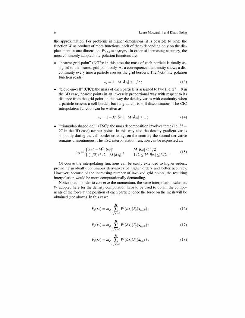
the approximation. For problems in higher dimensions, it is possible to write thefunction W as product of more functions, each of them depending only on the dis-placement in one dimension: Wi, j,k = wiw jwk. In order of increasing accuracy, themost commonly adopted interpolation functions are:

• “nearest-grid-point” (NGP): in this case the mass of each particle is totally as-signed to the nearest grid point only. As a consequence the density shows a dis-continuity every time a particle crosses the grid borders. The NGP interpolationfunction reads:

wi = 1, M |)xi|# 1/2 ; (13)

• “cloud-in-cell” (CIC): the mass of each particle is assigned to two (i.e. 23 = 8 inthe 3D case) nearest points in an inversely proportional way with respect to itsdistance from the grid point: in this way the density varies with continuity whena particle crosses a cell border, but its gradient is still discontinuous. The CICinterpolation function can be written as:

wi = 1!M |)xi| , M |)xi|# 1 ; (14)

• “triangular-shaped-cell” (TSC): the mass decomposition involves three (i.e. 33 =27 in the 3D case) nearest points. In this way also the density gradient variessmoothly during the cell border crossing; on the contrary the second derivativeremains discontinuous. The TSC interpolatation function can be expressed as:

wi =#

3/4!M2 |)xi|2 M |)xi|# 1/2(1/2)(3/2!M |)xi|)2 1/2#M |)xi|# 3/2

. (15)

Of course the interpolating functions can be easily extended to higher orders,providing gradually continuous derivatives of higher orders and better accuracy.However, because of the increasing number of involved grid points, the resultinginterpolation would be more computationally demanding.

Notice that, in order to conserve the momentum, the same interpolation schemesW adopted here for the density computation have to be used to obtain the compo-nents of the force at the position of each particle, once the force on the mesh will beobtained (see above). In this case:

Fx(xl) = mp

M

#i, j,k=1

W ()xl)Fx(xi, j,k) ; (16)

Fy(xl) = mp

M

#i, j,k=1

W ()xl)Fy(xi, j,k) ; (17)

Fz(xl) = mp

M

#i, j,k=1

W ()xl)Fz(xi, j,k) . (18)


2.3.2 Poisson equation

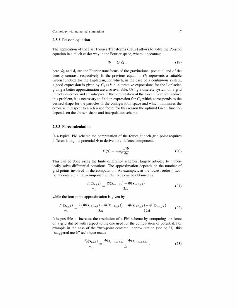
The application of the Fast Fourier Transforms (FFTs) allows to solve the Poissonequation in a much easier way in the Fourier space, where it becomes:

#k = Gk)k ; (19)

here #k and )k are the Fourier transforms of the gravitational potential and of thedensity contrast, respectively. In the previous equation, Gk represents a suitableGreen function for the Laplacian, for which, in the case of a continuous system,a good expression is given by Gk " k!2; alternative expressions for the Laplaciangiving a better approximation are also available. Using a discrete system on a gridintroduces errors and anisotropies in the computation of the force. In order to reducethis problem, it is necessary to find an expression for Gk which corresponds to thedesired shape for the particles in the configuration space and which minimizes theerrors with respect to a reference force: for this reason the optimal Green functiondepends on the chosen shape and interpolation scheme.

2.3.3 Force calculation

In a typical PM scheme the computation of the forces at each grid point requiresdifferentiating the potential # to derive the i-th force component:

Fi(x) =!mpd#dxi

. (20)

This can be done using the finite difference schemes, largely adopted to numer-ically solve differential equations. The approximation depends on the number ofgrid points involved in the computation. As examples, at the lowest order (“two-point centered”) the x-component of the force can be obtained as:

Fx(xi, j,k)mp

=#(xi!1, j,k)!#(xi+1, j,k)

2&, (21)

while the four-point approximation is given by

Fx(xi, j,k)mp

=2$#(xi+1, j,k)!#(xi!1, j,k)

%

3&!

#(xi+2, j,k)!#(xi!2, j,k)12&

. (22)

It is possible to increase the resolution of a PM scheme by computing the forceon a grid shifted with respect to the one used for the computation of potential. Forexample in the case of the “two-point centered” approximation (see eq.21), this“staggered mesh” technique reads:

Fx(xi, j,k)mp

=#(xi!1/2, j,k)!#(xi+1/2, j,k)

&. (23)


It is well known that the finite difference schemes introduce truncation errors inthe solutions. A way to avoid this problem and to gain a better accuracy is to obtainthe forces directly from the gravitational potential in Fourier space: Fk =!ik#k. Inthis case it is necessary to inverse-transform separately each single component ofthe force, using more frequently the FFT routines.

2.3.4 Pros and cons

The big advantage of the PM method is its high computational speed: in fact thenumber of operations scales as Np +Nglog(Ng), where Np is the number of particlesand Ng = M3 the number of grid points. The small dynamical range, strongly lim-itated by the number of grid points and by the corresponding memory occupation,represents the largest problem of the method: only adopting hybrid methods (seeabove), it is possible to reach the sufficient resolution necessary in cosmologicalsimulations.

2.4 Tree codes

Thanks to its computational performance and accuracy, this method represents todaythe favorite tool for cosmological N-body simulations. The idea to solve the N-bodyproblem is based on the exploitation of a hierarchical multipole expansion, the so-called tree algorithm. The speed up is obtained by using, for sufficiently distantparticles, a single multipole force, in spite of computing every single distance, asrequired for methods based on direct sum. In this way the sum ideally reduces toNp log(Np) operations, even if, for gravitationally evolved structures, the scalingcan be less efficient.

In practice, the multiple expansion is based on a hierarchical grouping that isobtained, in the most common algorithms, by subdividing in a recursive way thesimulation volume. In the approach suggested by [2] a cubical root node is usedto encompass the full mass distribution. This cube is then repeatedly subdividedinto eight daughter nodes of half the side-length each, until one ends up with ‘leaf’nodes containing single particles. The computation of the force is then done by“descending” the tree. Starting from the root node, the code evaluates, by applyinga suitable criterion, whether or not the multipole expansion of the node providesan accurate enough partial force: in case of a positive answer, the tree descent isstopped and the multipole force is used; in the negative case, the daughter nodes areconsidered in turn. Usually the opening criterion is based on a given fixed angle,whose choice controls the final error: typically one assumes the angle to be $ 0.5rad. Obviously, the smaller and the more distant the particles’ groups, the moreaccurate the assumption of multipole expansion.


2.5 Hybrid methods

Having the previous techniques quite different numerical properties with oppositepros and cons, it is possible to combine them to build new algorithms (called hy-brid methods), possibly mantaining the positive aspects only. A first attempt hasbeen done with the P3M code, which combines the high accuracy of the direct sumimplemented by the PP method at small scale with the speed of the PM algorithmto compute the large-scale interactions. An improved version of this code has beenalso proposed, where spatially adaptive mesh refinements are possible in regions atvery high density. This algorithm, called AP3M [6], has been used to run severalcosmological simulations, including the Hubble Volume simulations [9].

In the last-generation codes like GADGET[23], hybrid codes are built by re-placing the direct sum with tree algorithms: the so-called TreePM. In this case, thepotential is explicitly split in Fourier space into a long-range and a short-range partaccording to #k = # long

k +# shortk , where

# longk = #k exp(!k2r2

s ) ; (24)

here rs corresponds to the spatial scale of the force-split. The long-range potentialcan be computed very efficiently with mesh-based Fourier methods, like in the PMmethod. The short-range part of the potential can be solved in real space by notingthat for rs % L the short-range part of the real-space solution of the Poisson equationis given by

# short(x) =!G#i

mi

rierfc

&ri

2rs

'. (25)

In the previous equation ri is the distance of any particle i to the point x. Thus theshort-range force can be computed adopting the tree algorithm, except that the forcelaw is modified by a long-range cut-off factor.

This approach allows to largely improve the computational performance com-pared to ordinary tree methods, maintaining all their advantages: the very large dy-namical range, the insensitivity to clustering, and the precise control of the softeningscale of the gravitational force.

2.6 Initial conditions and simulation setup

As said, the N-body simulations are a tool often used to produce, once a given cos-mological model is assumed, the predictions, which can be directly compared to realobservational data to falsify the model itself. For this reason it is necessary to have arobust method to assign to the Np particles the correct initial conditions, correspond-ing to a fair realisation of the desired cosmological model. The standard inflationaryscenarios predict that the initial density fluctuations are a random field with an al-most Gaussian distribution (for non-Gaussian models and the corresponding initial


conditions, see for example [11]). In this case the field is completely defined by itspower spectrum P(k), whose shape is related to the choices made about the under-lying cosmological model and the nature of dark matter.

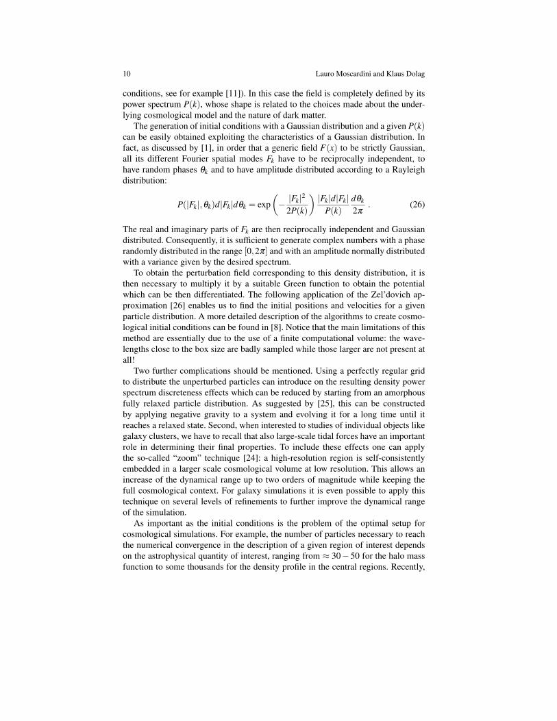
The generation of initial conditions with a Gaussian distribution and a given P(k)can be easily obtained exploiting the characteristics of a Gaussian distribution. Infact, as discussed by [1], in order that a generic field F(x) to be strictly Gaussian,all its different Fourier spatial modes Fk have to be reciprocally independent, tohave random phases *k and to have amplitude distributed according to a Rayleighdistribution:

P(|Fk|,*k)d|Fk|d*k = exp&! |Fk|2

2P(k)

'|Fk|d|Fk|

P(k)d*k

2$. (26)

The real and imaginary parts of Fk are then reciprocally independent and Gaussiandistributed. Consequently, it is sufficient to generate complex numbers with a phaserandomly distributed in the range [0,2$] and with an amplitude normally distributedwith a variance given by the desired spectrum.

To obtain the perturbation field corresponding to this density distribution, it isthen necessary to multiply it by a suitable Green function to obtain the potentialwhich can be then differentiated. The following application of the Zel’dovich ap-proximation [26] enables us to find the initial positions and velocities for a givenparticle distribution. A more detailed description of the algorithms to create cosmo-logical initial conditions can be found in [8]. Notice that the main limitations of thismethod are essentially due to the use of a finite computational volume: the wave-lengths close to the box size are badly sampled while those larger are not present atall!

Two further complications should be mentioned. Using a perfectly regular gridto distribute the unperturbed particles can introduce on the resulting density powerspectrum discreteness effects which can be reduced by starting from an amorphousfully relaxed particle distribution. As suggested by [25], this can be constructedby applying negative gravity to a system and evolving it for a long time until itreaches a relaxed state. Second, when interested to studies of individual objects likegalaxy clusters, we have to recall that also large-scale tidal forces have an importantrole in determining their final properties. To include these effects one can applythe so-called “zoom” technique [24]: a high-resolution region is self-consistentlyembedded in a larger scale cosmological volume at low resolution. This allows anincrease of the dynamical range up to two orders of magnitude while keeping thefull cosmological context. For galaxy simulations it is even possible to apply thistechnique on several levels of refinements to further improve the dynamical rangeof the simulation.

As important as the initial conditions is the problem of the optimal setup forcosmological simulations. For example, the number of particles necessary to reachthe numerical convergence in the description of a given region of interest dependson the astrophysical quantity of interest, ranging from $ 30!50 for the halo massfunction to some thousands for the density profile in the central regions. Recently,


[19] presented a comprehensive series of convergence tests designed to study theeffect of numerical parameters on the structure of simulated dark matter haloes. Inparticular the paper discusses the influence of the gravitational softening, the timestepping algorithm, the starting redshift, the accuracy of force computations, and thenumber of particles in the spherically-averaged mass profile of a galaxy-sized halo.The results were summarized in empirical rules for the choice of these parametersand in simple prescriptions to assess the effective convergence of the mass profileof a simulated halo, when computational limitations are present.

In general, it is important to notice that both the size and the dynamical range orresolution of the N-body simulations have been increasing very rapidly over the lastdecades, in a way that, thanks to improvements in the algorithms, is faster than theunderlying growth of the available CPU power.

2.7 Code comparison

Thanks the analysis of very recent data regarding the cosmic microwave back-ground, the galaxy surveys and the high-redshift supernovae, we entered the eraof the so-called high-precision cosmology, with very stringent constraints (i.e. atthe per cent accuracy level) on the main parameters. In the perspective of even bet-ter data as expected in upcoming projects, the theoretical predictions, in order tobe a useful and complementary tool, must reach a similar level of precision, that,particularly in the highly non-linear regime, represents a real challenge.

A first step in this direction is the launch of an extensive program of comparisonbetween the different numerical codes available in the community. An example isthe work presented in [12], where ten different codes adopting a variety of schemes(tree, APM, tree-PM, etc.) have been tested against the same initial conditions. Ingeneral the comparison has been very satisfactory, even if the variance betweenthe results is still too large to make predictions suitable for the next-generation ofgalaxy surveys. In particular the accuracy in the determination of the halo massfunction is always better than 5 per cent, while the agreement for the power spectrumin the nonlinear regime is at the 5! 10 per cent level, even on moderate spatialscales around k = 10h Mpc!1. Considering the internal structure of halos in the outerregions of & R200, it also appears to be very similar between different simulationcodes. Larger differences between the codes in the inner region of the halos occuronly if the halo is not in a relaxed state.


3 Hydrodynamical codes

3.1 The model equations

Even if the dark matter component represents the dominant contribution to the totalmatter distribution in the universe, it is quite important to have also a fair represen-tation of baryons: in fact most of the astrophysical signals are originated by physicalprocessed related to them.

In general the description of the baryonic component is based on the assumptionof an ideal fluid, for which the time evolution is obtained by solving the followingset of hydrodynamical equations: the Euler equation,

dvdt

=!!P%!!# ; (27)

the continuity equation,d%dt

+%!v = 0; (28)

the first law of thermodynamics,

dudt

=!P%

! ·v. (29)

In the previous equations, P and u represent the pressure and the internal energy(per unit mass), that under the assumption of an ideal monatomic gas, are related bythe equation of state: P = 2/3%u. Notice that for the moment we neglect the effectproduced by radiative losses, usually encrypted by the cooling function +(u,%) (seethe discussion in Section 3.5).

In the recent years, different techniques have been proposed to solve the cou-pled equations of dark and baryonic matter. All of them treat the gravitational termrelated to !# with the same kinds of technique described in the previous section.For the hydrodynamical part they adopt different strategies which can be classifiedin two big categories: lagrangian and eulerian techiques. The former are methodsbased on a finite number of particles used to describe the mass distribution, whilethe latter are methods that adopt a mesh to discretize the simulation volume. Be-fore reviewing in the following subsections the main characteristics of their mostimportant prototypes, we notice here that considering self-gravity, as necessary incosmological applications, introduces a much higher level of complexity, with re-spect to standard hydrodynamical simulations. In fact the formation of very evolveddensity structures induces motions which are often extremely supersonic, whith thepresence of shocks and discontinuities. Moreover, in order to have reliable simu-lations, the process of structure formation must be accurately followed on a verylarge range of scales, covering many order of magnitudes in space, in time and inthe interesting physical quantities (temperature, pressure, energy, etc.). Finally, weneed to include the expansion of the universe, which modifies the previous set of


equations as:"v" t

+1a(v ·!)v+

aa

v =! 1a%

!P! 1a

!# , (30)

"%" t

+3aa

% +1a

! · (%v) = 0 (31)

and"" t

(%u)+1a

v ·!(%u) =!(%u+P)&

1a

! ·v+3aa

'. (32)

3.2 Smoothed Particle Hydrodynamics (SPH)

The most popular lagrangian method is certainly SPH, that has a very good spatialresolution in high-density regions, while its performance in underdense region isunsatisfactory. Another charcateristic of SPH is the fact that it adopts an artificialviscosity which does not allow to reach a sufficiently high resolution in shockedregion. Even if in general it is not able to treat dynamical instabilities with the sameaccuracy of the eulerian methods presented in the next subsection, thanks to itsadaptive nature, SPH is still the preferred method for cosmological hydrodynamicalsimulations.

Here we introduce the basic idea of the technique. We refer to [16] for a moreextended presentation of the method. Unlike in the eulerian algorithms, in SPH thefluid is represented using mass elements, i.e. a finite set of particles. This choiceoriginates the different performance in high- and low-density regions: in fact wherethe mean interparticle distance is smaller, the fluid is less sparsely sampled, with aconsequent better resolution; the opposite holds when the interparticle distance islarge.

3.2.1 Basics of SPH

As said, in SPH the fluid is discretized using mass elements (i.e. a finite set ofparticles), unlike in eulerian codes where the discretization is made using volumeelements. Thanks to an adaptive smoothing, the mass resolution is kept fixed. Inmore detail, a generic fluid quantity A is defined as

'A(x)(=!

W (x!x),h)A(x))dx), (33)

where the smoothing kernel W is suitably normalised:(

W (x,h)dx = 1. MoreoverW , assumed to depend only on the distance modulus, collapses to a delta function ifthe smoothing length h tends to zero.

Using a set of particles with mass m j and position x j, the previous integral canbe done in a discrete way, replacing the volume element of the integration with the


ratio of the mass and density m j/% j of the particles:

'Ai(= #j

m j

% jA jW (xi!x j,h) . (34)

If one adopts kernels with a compact support (i.e. W (x,h) = 0 for |x| > h), it isnot necessary to do the summation over the whole set of particles, but only over theneighbours around the i-th particle under consideration, namely the ones inside asphere of radius h. The following kernel represents an optimal choice in many casesand it has been used often in the literature:

W (x,h) =8

$h3

)*+

*,

1!6$ x

h%2 +6

$ xh%3 0# x/h < 0.5

2$1! x

h%3 0.5# x/h < 1

0 1# x/h. (35)

If the quantity A is the density %i, Eq. 34 becomes simpler:

'%i(= #j

m jW (xi!x j,h). (36)

The big advantage of SPH is that the derivatives can be easily calculated as

!'Ai(= #j

m j

% jA j!iW (xi!x j,h), (37)

where !i denotes the derivative with respect to xi. A pairwise symmetric formula-tion of derivatives can be obtained by exploiting the identity

(%!) ·A = !(% ·A)!% · (!A), (38)

which allows one to re-write a derivative as

!'Ai(=1%i

#j

m j(A j!Ai)!iW (xi!x j,h). (39)

Another symmetric representation of the derivative can be alternatively obtainedfrom the identity

!A%

= !&

A%

'+

A%2 !%, (40)

which then leads to:

!'Ai(= %i #j

m j

-A j

%2j+

Ai

%2i

.!iW (xi!x j,h). (41)

By applying the previous identities, one can re-write the Euler equation as


dvi

dt=!#

jm j

-Pj

%2j+

Pi

%2i

+,i j

.!iW (xi!x j,h), (42)

while the term !(P/%)! ·v in the first law of thermodynamics can be written as

dui

dt=

12 #

jm j

-Pj

%2j+

Pi

%2i

+,i j

.(v j!vi)!iW (xi!x j,h). (43)

In order to have a good reproduction of shocks, in the previous equations it hasbeen necessary to introduce the so-called artificial viscosity ,i j, for which differentforms have been proposed in the literature (see, for example, [17]): most of themtry to reduce its effects in the regions where there are no shocks, adopting a specificarticial viscosity for each particle.

To complete the set of fluid equations, we notice that the continuity equationdoes not represent a problem for Lagrangian methods like SPH, being automaticallysatisfied thanks to the conservation of the number of particles.

3.2.2 The smoothing length

Usually, each individual particle i has its own smoothing length h, which is de-termined by finding the radius hi of a sphere which contains Nnei neighbours. Alarge value for Nnei would allow better estimates for the density field but withlarger systematics; viceversa small Nnei would lead to larger sample variances.In the literature standard choices for Nnei range between 32 and 100. The pres-ence of a variable smoothing length in the hydrodynamical equations can breaktheir conservative form: to avoid it, it is necessary to introduce a symmetric kernelW (xi ! x j,hi,h j) = Wi j, for which the two main variants used in the literature arethe kernel average,

Wi j = (W (xi!x j,hi)+W (xi!x j,h j))/2 , (44)

and the average of the smoothing lengths

Wi j = W (xi!x j,(hi +h j)/2) . (45)

Note that when writing the derivatives, we assumed that h is independent of theposition x j. Thus, if the smoothing length hi is variable for each particle, one wouldformally introduce the correction term "W/"h in all the derivatives. An elegant wayto do that is using the formulation which conserves numerically both entropy andinternal energy, described in the next subsection.


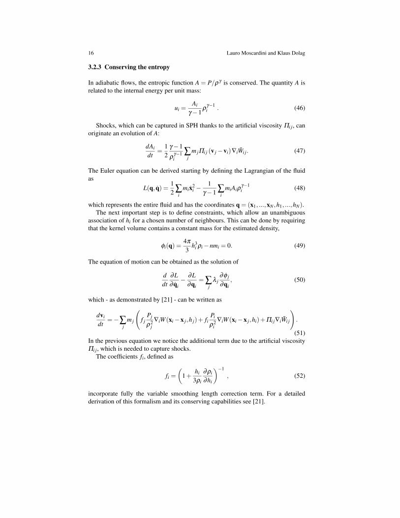
3.2.3 Conserving the entropy

In adiabatic flows, the entropic function A = P/%- is conserved. The quantity A isrelated to the internal energy per unit mass:

ui =Ai

-!1%-!1

i . (46)

Shocks, which can be captured in SPH thanks to the artificial viscosity ,i j, canoriginate an evolution of A:

dAi

dt=

12

-!1%-!1

i#

jm j,i j (v j!vi)!iWi j. (47)

The Euler equation can be derived starting by defining the Lagrangian of the fluidas

L(q, q) =12 #

imix2

i !1

-!1 #i

miAi%-!1i (48)

which represents the entire fluid and has the coordinates q = (x1, ...,xN ,h1, ...,hN).The next important step is to define constraints, which allow an unambiguous

association of hi for a chosen number of neighbours. This can be done by requiringthat the kernel volume contains a constant mass for the estimated density,

.i(q) =4$3

h3i %i!nmi = 0. (49)

The equation of motion can be obtained as the solution of

ddt

"L" qi

! "L"qi

= #j

/ j". j

"qi, (50)

which - as demonstrated by [21] - can be written as

dvi

dt=!#

jm j

-f j

Pj

%2j

!iW (xi!x j,h j)+ fiPi

%2i

!iW (xi!x j,hi)+,i j!iWi j

..

(51)In the previous equation we notice the additional term due to the artificial viscosity,i j, which is needed to capture shocks.

The coefficients fi, defined as

fi =&

1+hi

3%i

"%i

"hi

'!1, (52)

incorporate fully the variable smoothing length correction term. For a detailedderivation of this formalism and its conserving capabilities see [21].


3.3 Eulerian methods

These methods solve the hydrodynamical equations adopting a grid, which can befixed or adaptive in time. The first attempts were based on the so-called central dif-ference schemes, i.e. schemes where the relevant hydrodynamical quantities wereonly represented by their values at the center of the grid, and the various deriva-tives were obtained by the finite-difference representation. This approach was notsatisfactory: in fact the schemes were only first-order accurate and they made use ofsome artificial viscosity to treat discontinuities, similarly to SPH. In more moderncodes (like for example the piecewise parabolic method, PPM) the shape of the hy-drodynamical quantities fn,u(x) is recovered with much higher accuracy thanks tothe use of several neighbouring cells. This allows to calculate the total integral ofthe given quantity over the grid cell, divided by the volume of each cell (e.g. cellaverage, un), rather than pointwise approximations at the grid centres (e.g. centralvariables, un):

un =xn+0.5!

xn!0.5

fn,u(x)dx . (53)

This global shape is also used to estimate the values at the cell boundaries (e.g.ul

n±0.5,urn±0.5, the so-called interfaces), which can be used later as initial conditions

of a Riemann problem, e.g. the evolution of two constant states separated by a dis-continuity. Once the Riemann is analytically solved (see, e.g., [7]), it is possible tocompute the fluxes across these boundaries for the time interval and then to updatethe cell averages un. Notice that for high-dimensional problems, this procedure hasto be repeated for each coordinate direction separately.

In general, the eulerian methods suffer from limited spatial resolution, but theywork extremely well in both low- and high-density regions, as well as in treatingshocks. In cosmological simulations, accretion flows with large Mach numbers arevery common. Here, following the total energy in the hydrodynamical equations canproduce inaccurate thermal energy, leading to negative pressure, due to discretisa-tion errors when the kinetic energy dominates the total energy. In such cases, thenumerical schemes usually switch from formulations solving the total energy to for-mulations based on solving the internal energy in these hypersonic flow regions.

3.4 Code Comparison

The hydrodynamical schemes presented in the previous sections are based on quitedifferent approaches, having for construction very different characteristics (in prac-tice particles against grid). For this reason, in order to be validated, they must betested against problems with known solutions and then one has to compare theirresults, once the same initial conditions are given. The first standard test is the re-production of the shock tube problem: in this case codes able to capture the presence


of shocks, like the most sophisticated eulerian methods, have certianly better perfor-mances. Another possible test is the evolution of an initially spherical perturbation.

In general, a code validation in a more cosmological context is difficult. A firstattempt of comparison between grid-based and SPH-based codes can be found in[14]. More recently [18] compared the thermodynamical properties of the inter-galactic medium predicted by the lagrangian code GADGET and by the euleriancode ENZO.

In the case of simulations for single cosmic structures, the most complete codecomparison is the one provided by the Santa Barbara Cluster Comparison Project[10], where 12 different groups ran the own codes (including both eulerian and la-grangian schemes), starting from the same identical initial conditions correspondingto a massive galaxy cluster. In general the agreement for the dark matter propertieswas satisfactory, with a 20 per cent scatter around the mean density and velocitydispersion profiles. A similar agreement was also obtained for many of the gasproperties, like the temperature profile or the ratio of the specific dark matter ki-netic energy to the gas thermal energy; somewhat larger differences are found in thetemperature or entropy profiles in the innermost regions. One of the most worry-ing discrepancies is certainly when the total X-ray luminosity is considered: in thiscase the spread can be also a factor 10. Most of the problem originates from a toolow resolution in the central core, where the gas density (which enters as squaredin the estimate of the X-ray luminosity) reaches its maximum. Another large differ-ence between the results of different hydro-codes is related to the predicted baryonfraction and its profile within the cluster.

In general we can conclude that lagrangian and eulerian schemes are providingcompatible results, with some spread due to their specific weaknesses. However, wehave to remind that these comparisons have been done in the non-radiative regime,i.e. excluding a long list of complex physical processes acting on baryons (see thefollowing section), processes whose implementation is mandatory for a completedescription of the formation of cosmic structures.

3.5 Extra gas physics

We know very well that the formation and evolution of cosmic structures is not de-termined only by the gravity due to the total matter distribution and by the adiabaticbehaviour of gas: many other important processes are in action, in particular on thebaryonic component, influencing the final (physical and observational) properties ofthe structures. Here we briefly list these processes, discussing their importance andpointing out the related numerical issues.

• Cooling. Its standard implementation is made by adding the cooling function+(u,%) in the first law of thermodynamics, under the assumptions that the gasis optically thin and in ionisation equilibrium, and that only two-body coolingprocesses are important. Considering a plasma with primordial composition ofH and He, these processes are collisional excitation of H I and He II, collisional


ionisation of H I, He I and He II, standard recombination of H II, He II and He III,dielectric recombination of He II, and free-free emission (Bremsstrahlung). Be-ing the collisional ionisation and recombination rates depending only on the tem-perature, when the presence of a ionising background radiation is excluded it ispossible to solve the resulting rate equation analytically; alternatively the solu-tion is obtained iteratively (see a discussion in [15]). When also the metallicity isimplemented in the code, the number of possible processes becomes so large thatit is necessary to use pre-computed tabulated cooling function. Finally we noticethat for pratical reasons the gas cooling is followed as “sub time step” problem,decoupled from the hydrodynamical treatment.

• Star formation. The inclusion of the cooling process originates two numericalproblems. First, since the cooling is a runaway process, in the central regionsof clusters the typical cooling time becomes significantly shorter than the Hub-ble time, causing the so-called overcooling problem: the majority of baryons cancool down and condense out of the hot phase. Second, since cooling is propor-tional to the square of the gas density, its efficiency is strongly related to thenumber of the first collapsed structures, whose good representation in simula-tions depends on the assumed numerical resolution. To avoid these problems, itis necessary to include the process of star formation starting from the cold anddense phase of the gas. These stellar objects, once the phase of supernova explo-sion is reached, can inject a large amount of energy (the so-called feedback) inthe gas, increasing its temperature and possibly counteracting the cooling catas-trophe. From a numerical point of view, this process is implemented via simplerecipes (see, for example, [15]), based on the assumptions that the gas has a con-vergent flow, it is Jeans unstable and, most important, it has an overdensity largerthan the threshold corresponding to collapsed regions. This procedure allows tocompute the fraction of gas converted into stars. For computational and numeri-cal reasons, the star formation is done only when a significant fraction of the gasparticle mass is interested by the transformation: at this point, a new collision-less “star” particle is created from the parent star-forming gas particle, whosemass is reduced accordingly. This process takes place until the gas particle is en-tirely transformed into stars. In order to avoid spurious numerical effects, whicharise from the gravitational interaction of particles with widely differing masses,one usually restricts the number of star particles spawned by a gas particle to berelatively small, typically 2!3.

• Supernova feedback. Assuming a specific initial mass function, it is possible toestimate the number of stars ending their lifes as type-II supernovae and then tocompute the total amount of energy (typically 1051 erg per supernova) that eachstar particle can release to the surrounding gas. Assuming that the typical lifetimeof massive stars is smaller than the typical simulation time step, the feedbackenergy is injected in the surrounding gas in the same step (instantaneous recy-cling approximation). Improvements with respect to this simple model includean explicit sub-resolution description of the multi-phase nature of the interstellarmedium, which provides the reservoir of star formation. Such a sub grid modeltries to model the global dynamical behaviour of the interstellar medium in which


cold, star-forming clouds are embedded in a hot medium (see for example theself-regulated model proposed by [22] and a general critical discussion in [4]). .

• Chemical enrichment. A possible way to improve the previous models is theinclusion of a more detailed description of stellar evolution, and of the corre-sponding chemical enrichment. In particular it is possible to follow the release ofmetals also from type-Ia supernovae and low and intermediate mass stars, avoid-ing the instantaneous recycling approximation (see the discussion in [5]).

• Other processes. The baryons present in the cosmic structures undergo otherphysical processes that can have an important role in their modelization: a nonexaustive list includes the effects related to thermal conduction, radiative transfer,magnetic fields, relativistic particles, black holes and extra sources of feedback(like, for instance, AGN). The first attempts of implementing the correspond-ing physics in cosmological simulations have been done, even if in some casesthe results are not yet convergent. Having a robust implementation of all thesephenomena represents the more difficult and changelling frontier for future nu-merical experiments.

References

1. Bardeen, J. M., Bond, J. R., Kaiser, N., & Szalay, A. S. 1986, ApJ, 304, 152. Barnes, J., & Hut, P. 1986, Nature, 324, 4463. Binney, J., & Tremaine, S. 1987, Princeton, NJ, Princeton University Press, 19874. Borgani, S., et al. 2006, MNRAS, 367, 16415. Borgani, S., Fabjan, D., Tornatore, L., Schindler, S., Dolag, K., & Diaferio, A. 2008, Space

Science Reviews, 134, 3796. Couchman, H. M. P. 1991, ApJ, 368, L237. Courant, R., & Friedrichs, K. O. 1948, Pure and Applied Mathematics, New York: Inter-

science8. Efstathiou, G., Davis, M., White, S. D. M., & Frenk, C. S. 1985, ApJS, 57, 2419. Evrard, A. E., et al. 2002, ApJ, 573, 7

10. Frenk, C. S., et al. 1999, ApJ, 525, 55411. Grossi, M., Dolag, K., Branchini, E., Matarrese, S., & Moscardini, L. 2007, MNRAS, 382,

126112. Heitmann, K., et al. 2008, Computational Science and Discovery, 1, 01500313. Ito, T., Makino, J., Fukushige, T., Ebisuzaki, T., Okumura, S. K., & Sugimoto, D. 1993, PASJ,

45, 33914. Kang, H., Ostriker, J. P., Cen, R., Ryu, D., Hernquist, L., Evrard, A. E., Bryan, G. L., &

Norman, M. L. 1994, ApJ, 430, 8315. Katz, N., Weinberg, D. H., & Hernquist, L. 1996, ApJS, 105, 1916. Monaghan, J. J. 1992, ARA&A, 30, 54317. Monaghan, J. J. 1997, Journal of Computational Physics, 136, 29818. O’Shea, B. W., Nagamine, K., Springel, V., Hernquist, L., & Norman, M. L. 2005, ApJS, 160,

119. Power, C., Navarro, J. F., Jenkins, A., Frenk, C. S., White, S. D. M., Springel, V., Stadel, J.,

& Quinn, T. 2003, MNRAS, 338, 1420. Press, W. H., Teukolsky, S. A., Vetterling, W. T., & Flannery, B. P. 1992, Cambridge: Univer-

sity Press21. Springel, V., & Hernquist, L. 2002, MNRAS, 333, 649


22. Springel, V., & Hernquist, L. 2003, MNRAS, 339, 28923. Springel, V. 2005, MNRAS, 364, 110524. Tormen, G., Bouchet, F. R., & White, S. D. M. 1997, MNRAS, 286, 86525. White, S. D. M. 1996, Cosmology and Large Scale Structure, 34926. Zel’Dovich, Y. B. 1970, A&A, 5, 84

Cosmology with numerical simulations - ICCUBicc.ub.edu/~liciaverde/IC/como.pdf · Cosmology with...

Documents

Transcript of Cosmology with numerical simulations - ICCUBicc.ub.edu/~liciaverde/IC/como.pdf · Cosmology with...