Cosmology Group Presentation at York University

DynamicalSystems

Methods inEarly-UniverseCosmologies

Ikjyot SinghKohliPh.D.

CandidateYork

University

Outline

Introduction

Description ofthe Matter

Deriving theDynamicalEquations

The Theory ofOrthonormalFrames

DynamicalSystemsTechniques

Dynamical Systems Methods in Early-Universe

Cosmologies

Ikjyot Singh KohliPh.D. CandidateYork University

Wednesday, February 12, 2014

DynamicalSystems



CandidateYork

University

Outline

Introduction





1 Introduction

2 Description of the Matter

3 Deriving the Dynamical Equations

4 The Theory of Orthonormal Frames

5 Dynamical Systems Techniques

DynamicalSystems



CandidateYork

University

Outline

Introduction





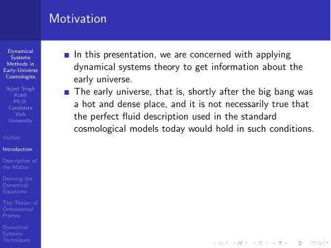
Motivation

In this presentation, we are concerned with applyingdynamical systems theory to get information about theearly universe.

DynamicalSystems



CandidateYork

University

Outline

Introduction





Motivation

In this presentation, we are concerned with applyingdynamical systems theory to get information about theearly universe.The early universe, that is, shortly after the big bang wasa hot and dense place, and it is not necessarily true thatthe perfect fluid description used in the standardcosmological models today would hold in such conditions.

DynamicalSystems



CandidateYork

University

Outline

Introduction





Motivation

In this presentation, we are concerned with applyingdynamical systems theory to get information about theearly universe.The early universe, that is, shortly after the big bang wasa hot and dense place, and it is not necessarily true thatthe perfect fluid description used in the standardcosmological models today would hold in such conditions.One has to account for potential anisotropic/dissipativeeffects which in fluid dynamics as characterized byviscosity.

DynamicalSystems



CandidateYork

University

Outline

Introduction





Motivation

In this presentation, we are concerned with applyingdynamical systems theory to get information about theearly universe.The early universe, that is, shortly after the big bang wasa hot and dense place, and it is not necessarily true thatthe perfect fluid description used in the standardcosmological models today would hold in such conditions.One has to account for potential anisotropic/dissipativeeffects which in fluid dynamics as characterized byviscosity.For a review of the justification of including viscosityterms in early-universe cosmological models see thearticles by Barrow (1988,1982) [3] [2] and the article byBelinskii and Khalatnikov (1976) [4].

DynamicalSystems



CandidateYork

University

Outline

Introduction





Motivation

In this presentation, we are concerned with applyingdynamical systems theory to get information about theearly universe.The early universe, that is, shortly after the big bang wasa hot and dense place, and it is not necessarily true thatthe perfect fluid description used in the standardcosmological models today would hold in such conditions.One has to account for potential anisotropic/dissipativeeffects which in fluid dynamics as characterized byviscosity.For a review of the justification of including viscosityterms in early-universe cosmological models see thearticles by Barrow (1988,1982) [3] [2] and the article byBelinskii and Khalatnikov (1976) [4].As a result, we will keep our assumption of the spatialhomogeneity of the early universe, but now assume it is

DynamicalSystems



CandidateYork

University

Outline

Introduction





Energy-Momentum Tensor Derivation I

In this section, we will derive the form of the requiredenergy-momentum tensor, namely, for that of a viscous fluidwithout heat conduction. Recall that the energy-momentumtensor for a perfect fluid takes the form

T ab = (µ + p)uaub − ucucgabp. (1)

For the moment, letting µ+ p = W, we obtain

T ab = Wuaub − ucucgabp, (2)

Denoting the viscous contributions by Vab, we seek amodification of Eq. (2) such that

Tab = Wuaub − ucucgabp + Vab. (3)

DynamicalSystems



CandidateYork

University

Outline

Introduction





Energy-Momentum Tensor Derivation II

To obtain the form of this additional tensor term, we note thatfrom classical fluid mechanics, the Euler equation is given as

(ρui),t = −Πik,k , (4)

where Πik is the momentum flux tensor. Also, recall that for anon-viscous fluid, one has the fundamental relationship

Πik = pδik + ρuiuk . (5)

We simply add a term to Eq. (5) that represents the viscousmomentum flux, Σik , to obtain

Πik = pδik + ρuiuk − Σik = −Sik + ρuiuk . (6)

It is important to note that

Sik = −pδik + Σik (7)

is the stress tensor, while, Σik is the viscous stress tensor.

DynamicalSystems



CandidateYork

University

Outline

Introduction





Energy-Momentum Tensor Derivation III

Note that, in what follows below, the viscous stress tensor,Σik , is not to be confused with Σik , the Hubble-normalizedshear tensor.

The general form of the viscous stress tensor can beformed by recalling that viscosity is formed when the fluidparticles move with respect to each other at differentvelocities, so this stress tensor can only depend on spatialcomponents of the fluid velocity.

We assume that these gradients in the velocity are small,so that the momentum tensor only depends on the firstderivatives of the velocity in some Taylor series expansion.

DynamicalSystems



CandidateYork

University

Outline

Introduction





Energy-Momentum Tensor Derivation IV

Therefore, Σik is some function of the ui ,k . In addition,when the fluid is in rotation, no internal motions ofparticles can be occurring, so we consider linearcombinations of ui ,k + uk,i , which clearly vanish for a fluidin rotation with some angular velocity, Ωi . The mostgeneral viscous tensor that can be formed is given by

Σik = η

!

ui ,k + uk,i −2

3δikul ,l

"

+ ξδikul ,l , (8)

where η and ξ are the coefficients of shear andbulk/second viscosity, respectively [15] [13].

DynamicalSystems



CandidateYork

University

Outline

Introduction





Energy-Momentum Tensor Derivation V

In Eq. (8), we note that δikul ,l is an expansion rate tensor,and

#

ui ,k + uk,i −23δikul ,l

$

represents the shear ratetensor. Since we would like to generalize this expression tothe general relativistic case, we replace the partialderivatives above with covariant derivatives, and theKroenecker tensor with a more general metric tensor, thatis, δik → gik .

We thus have that

Σik = η

!

ui ;k + uk;i −2

3gikul ;l

"

+ ξgikul ;l . (9)

Denoting the shear rate tensor as σab, and the expansionrate scalar as θ ≡ ua;a, Eq. (9) becomes

Vab = −2ησab − ξθhab. (10)

DynamicalSystems



CandidateYork

University

Outline

Introduction





Energy-Momentum Tensor Derivation VI

Since we are interested in the Hubble-normalized approach,we will make use of the definition θ ≡ 3H, where H is theHubble parameter. This means that Eq. (9) becomes

Vab = −2ησab − 3ξHhab. (11)

Substituting Eq. (11) into Eq. (3) we finally obtain therequired form of the energy-momentum tensor as

Tab = (µ+ p) uaub − ucucgabp − 2ησab − 3ξHhab. (12)

For simplicity, we shall let πab = −2ησab denote theanisotropic stress tensor, and commit to the metricsignature (−1,+1,+1,+1) such that Eq. (12) takes theform

Tab = (µ+ p) uaub + gabp − 3ξHhab + πab. (13)

DynamicalSystems



CandidateYork

University

Outline

Introduction





Basic Equations of Motion I

We will now derive the dynamical equations. Most of thisderivation follows from Ellis [6] and Grøn and Hervik [9], but Ihave tried to make thing slightly easier to understand. Let usfirst recall some basic properties of non-relativistic fluidmechanics. In fluid mechanics, we typically measure the fluidacceleration through the material derivative:

Dv

dt≡ v,t + (v ·∇)v, (14)

where v,t is the local derivative, and (v ·∇)v is known as theconvective derivative. Note that

Dva

dt= va,t + va,bx

b,t = va,t + vbva,b. (15)

DynamicalSystems



CandidateYork

University

Outline

Introduction





Basic Equations of Motion II

So we can write the convective term as Mv, where M = v i,j is amatrix, that is, it is the gradient of the velocity.We can now decompose v i,j into symmetric and anti-symmetricparts:

vi ,j = θij + ωij , (16)

where

θij =1

2

%

v i,j + v ji

&

(17)

is the expansion tensor and

ωij =

1

2

%

v i,j − v ji

&

(18)

is the vorticity tensor.

DynamicalSystems



CandidateYork

University

Outline

Introduction





Basic Equations of Motion III

I can now decompose the expansion tensor into trace andtrace-free parts:

θij =1

3θδij + σi

j , (19)

where

θ = v i,i , σij =

1

2

%

v i,j + v j,i

&

−1

3δij v

i,i . (20)

Note that σij is the trace-free tensor, and is known as the sheartensor. The shear tensor essentially measures deformations ofthe fluid.Combining all of these, I can essentially write:

vi ,j =1

3θδij + σij + ωij . (21)

DynamicalSystems



CandidateYork

University

Outline

Introduction





Basic Equations of Motion IV

Switching to the relativistic form we obviously have

aα = uα;mum = uα. (22)

We want to project the four-dimensional quantities onto thespatial slices and see how the evolve, these are our “dynamical”quantities. That is,

uα;β =1

3θhαβ + σαβ + ωαβ − uαuβ. (23)

Note that this last term is a consequence of purely relativisticeffects. It measures how much the fluid deviates from beinggeodesic. In our work, we always assume the fluid is geodesic,so the four-acceleration vanishes.

DynamicalSystems



CandidateYork

University

Outline

Introduction





Basic Equations of Motion V

We can write the energy-momentum tensor of the previoussection in the more general form:

Tuv = µuuuv + phuv + πuv . (24)

Using the properties that

πuu = 0, uuπuv = 0, (25)

and the Bianchi identities T vu;v = 0 imply that

uuT vu;v = 0

= uu#

µ,vuuuv + µuu;vu

v + µuuuv;u + hvu;vp + hvup,v

$

+ πvu;v

= −µ− θµ− θp − σuvπuv . (26)

DynamicalSystems



CandidateYork

University

Outline

Introduction





Basic Equations of Motion VI

Therefore, the energy conservation equation is

µ+ θ(µ+ p) + σuvπuv = 0, (27)

DynamicalSystems



CandidateYork

University

Outline

Introduction





To close this system, we need dynamical equations for θ andσuv . The idea for using kinematics to describe the dynamics ofuniverses obeying the Einstein field equations was firstintroduced by Trumper as mentioned in Hawking’s 1966 paper[10] and in Ellis’ Cargese Lectures [6].

DynamicalSystems



CandidateYork

University

Outline

Introduction





The Raychaudhuri Equation I

The basic defining equation for General Relativity is the Ricciidentity. Let us start with:

−uuuvRaubv = uvRauvbuu . (28)

I will write this as

−uuuvRaubv = ua;bvuv + ua;vu

v;b. (29)

If I now contract this equation, I obtain

− uuuvRuv = ub;bvuv + ua;vu

v ;a. (30)

If I now substitute the Einstein field equations

Rab = Tab −1

2T cc gab. (31)

DynamicalSystems



CandidateYork

University

Outline

Introduction





The Raychaudhuri Equation II

into the Ricci identity Eq. (30) and take the symmetric andtrace-free part, I obtain the shear-propagation equations:

hachbd σ

cd = −2Hσab − σacσ

bc −1

3

#

−2σ2$

hab +1

2πab (32)

If I take the trace of Eq. (30), I get the Raychaudhuri equation:

θ +1

3θ2 + σabσ

ab +1

2(µ+ 3p) = 0. (33)

The assumption that ua = 0 implies that ωuv = 0. In the 3 + 1formalism, one can show that

ua;b = Kab, (34)

DynamicalSystems



CandidateYork

University

Outline

Introduction





The Raychaudhuri Equation III

where Kab is the extrinsic curvature tensor. Gauss’ theoremegregium (Page 171, [9]) states that

(n+1)R =(n) R +%

K 2 − K abKab

&

+ 2(−1)(n+1)Rabuaub. (35)

Combining this with the Einstein field equations, we get:

T abuaub =1

2

%

(3)R − K abKab + K 2&

. (36)

If we now use Eqs. (23) and (24), we get the Friedmannequation:

1

3θ2 =

1

2σabσ

ab −1

2

(3)

R + µ. (37)

This is a constraint equation on initial conditions as we will seelater.

DynamicalSystems



CandidateYork

University

Outline

Introduction





The Raychaudhuri Equation IV

Note that, we still have a problem in that we really have notsimplified things much. Looking at the shear propagationequation (32), for example, we have that

σab ≡ σab;mum, (38)

which contains the covariant derivative, which contains theChristoffel symbols, so we still need to work with the metrictensor. This is where the grand theory of orthonormal framescomes in!

DynamicalSystems



CandidateYork

University

Outline

Introduction





Orthonormal Frame Formalism I

The idea of orthonormal frames is based on the groundbreaking1969 paper from Ellis and MacCallum [8], “A Class ofHomogeneous Cosmological Models”. First, what do we meanwhen we say a space-time is spatially homogeneous? Let M bea manifold with metric tensor g. The isometry group is definedby

Isom(M = φ : M → M|φ, isometry, (39)

that is φ∗g = g, i.e., the metric is left unchanged after applyingan isometry. This isometry group is a Lie group, and the groupgenerators are Killing vectors. These Killing vectors span afinite-dimensional space (the tangent space to the Lie group),and we define the isotropy subgroup of a point p ∈ M by

fp(M) = φ ∈ Isom(M)|φ(p) = p. (40)

DynamicalSystems



CandidateYork

University

Outline

Introduction





Orthonormal Frame Formalism II

So a homogenous space is one that for each pair of pointsa, b ∈ M, there exists a φ ∈ Isom(M) such that φ(p) = q.For such a homogeneous space, there exists a set of Killingvector fields ζi such that

[ζi , ζj ] = Dkij ζk . (41)

At a point p ∈ M, choose a basis set of vectors ei . It can beshown that the frame ei span a Lie algebra:

[ei , ej ] = C kij ek . (42)

Therefore, to construct a homogeneous space, one takes theC kij as the structure constants of the Lie algebra, and defines a

DynamicalSystems



CandidateYork

University

Outline

Introduction





Orthonormal Frame Formalism III

left-invariant frame by the above relation. For a dual basis, ωk

to ek , using the Cartan calculus, we have that

dwk = −1

2C kij ω

i ∧ ωj . (43)

Using these invariant one-forms, we can define the spatialmetric as

ds2 = gijωi ⊗ ωj , (44)

where the gij are constants. The amazing thing is that theKilling vectors are ζi , and the basis vectors are ej , that is, wecan just read them off!To proceed further, we also need to modify what we mean by aconnection on the manifold. First, consider a vector field u.We have for any scalar function g that

u(g) = umem(f ). (45)

DynamicalSystems



CandidateYork

University

Outline

Introduction





Orthonormal Frame Formalism IV

Now defineuv(g) = umem(v

nen(g)), (46)

which is

uv(g) = umem(vn)en(g) + umunemen(g). (47)

This is clearly not a vector, since it has second-order partialderivatives. However,

[u, v] = [umem(vn)− vmem(u

n)] en + umun [em, en] (48)

is indeed a vector. For an arbitrary basis,

[em, en] = cpuvep. (49)

These structure coefficients obviously vanish in a coordinatebasis, which is what most cosmologists usually work in.

DynamicalSystems



CandidateYork

University

Outline

Introduction





Orthonormal Frame Formalism V

We will also make use of a generalized connection ∇ thatassociates ∇XY to any two vector fields X and Y. In a generalbasis, we have that

∇vem = Γamnea, (50)

that is, the connection coefficients are defined as thecomponents of the directional derivative of the basis vectors.For more information, see [9] and Abraham and Marsden’sbook [1]. For two vector fields, X = Xmem, and u = umem, wehave that

∇uX = (en(Xm)un + X aΓmanu

v ) em. (51)

The commutator above therefore can now be written as:

[u, v] = ∇uv −∇vu+ (Γpmn − Γpnm + cpmn) umunep . (52)

DynamicalSystems



CandidateYork

University

Outline

Introduction





Orthonormal Frame Formalism VI

We defined the Torsion to be

T(u ∧ v) ≡ ∇uv −∇vu− [u, v] . (53)

We require spacetime in General Relativity to be torsion-free,so we have

camn = Γanm − Γamn. (54)

That is, all of the connection coefficients are now functions ofthe structure constants!In an orthonormal basis, gab = diag(−1, 1, 1, 1), so

Γamn =1

2

%

gabcbnm + gmbc

ban − gnbc

bma

&

. (55)

These are antisymmetric in the first two indices, so we canwrite:

Γabt = −Γbat ≡ ϵabcΩc , (56)

DynamicalSystems



CandidateYork

University

Outline

Introduction





Orthonormal Frame Formalism VII

where Ωc denotes the rotation of the spatial frame and isdefined by

Ωa =1

2ϵabgdubeg · ed . (57)

We can therefore write that

catb = −θab + ϵabcΩc . (58)

The rest of the structure coefficients are all spatial in nature,and we can write

ckij = ϵijlnlk + al

%

δki δlj − δkj δ

li

&

, (59)

where nlk and ai classify the Bianchi algebra, per the Behrdecomposition (See Stephani, Kramer, MacCallum,Hoenselaers, and Herit [16]), Landau and Liftshitz [14], Grønand Hervik [9] for a further explanation:

DynamicalSystems



CandidateYork

University

Outline

Introduction





Orthonormal Frame Formalism VIII

Group Class Group Type n11 n22 n33 Contains FLRW?A (ai = 0) I 0 0 0 k = 0

A II + 0 0A VI0 0 + -A VII0 0 + + k = 0A VIII - + +A IX + + + k = +1

B(ai = 0) V 0 0 0 k = −1B IV 0 0 +B VIh 0 + -B VIIh 0 + + k = −1

Table: The Bianchi classifications

DynamicalSystems



CandidateYork

University

Outline

Introduction





Orthonormal Frame Formalism IX

These classifications were due to Bianchi [5], but we follow theconventions of Ellis, Maartens and MacCallum. [7].One can find evolution equations for the nlk and the ai byrecognizing that the structure coefficients define a Lie algebra,so that the Jacobi identity holds. That is, for the set of vectors(u, ea, eb), we have that

0 = [u, [ea, eb]] + [ea, [eb ,u]] + [eb, [u, ea]]. (60)

Go through some algebra, actually a lot of algebra (!), and findthat we get

u(ckab) + cktdcdab + ckadc

dbt + ckbdc

dta = 0. (61)

DynamicalSystems



CandidateYork

University

Outline

Introduction





Orthonormal Frame Formalism X

Taking the trace of this equation, we get upon definingu = ∂/∂t that

ai = −1

3θai − σija

j − ϵijkajΩk , (62)

and the trace-free part yields

nab = −1

3θnab − 2nk(aϵb)klΩ

l + 2nk(aσkb). (63)

Returning to our propagation equations from before, we notethat for the shear propagation equation, we had

σab = um∇mσab = u(σab)− Γmanσmbun − Γmbnσamu

n. (64)

DynamicalSystems



CandidateYork

University

Outline

Introduction





Orthonormal Frame Formalism XI

Using the orthonormal frame formalism, we can write this as

σab = u (σab)− 2σd(aϵb)cdΩ

c . (65)

Setting a universal time gauge, u = ∂∂t and using the

convention that H = 13θ, (where H is the Hubble parameter)

we have the Einstein field equations in an orthonormal frame:

H = −H2 −2

3σ2 − µ

!

1

6+

1

2w

"

, (66)

σab = −3Hσab + 2ϵuv(a σb)uΩv − Sab − 2ησab, (67)

µ = 3H2 − σ2 +1

2R , (68)

0 = 3σua au − ϵuva σb

unbv , (69)

DynamicalSystems



CandidateYork

University

Outline

Introduction





Orthonormal Frame Formalism XII

where Sab and R are the three-dimensional spatial curvatureand Ricci scalar and are defined as:

Sab = bab −1

3buuδab − 2ϵuv(a nb)uav , (70)

R = −1

2buu − 6aua

u, (71)

where bab = 2nuanub − (nuu) nab. We have also denoted by Ωv

the angular velocity of the spatial frame.

nab = −Hnab + 2σu(anb)u + 2ϵuv(a nb)uΩv , (72)

aa = −Haaσbaab + ϵuva auΩv , (73)

0 = nbaab. (74)

DynamicalSystems



CandidateYork

University

Outline

Introduction





Orthonormal Frame Formalism XIII

The contracted Bianchi identities give the evolution equationfor µ as

µ = −3H (µ+ p)− σbaπ

ab + 2aaq

a. (75)

DynamicalSystems



CandidateYork

University

Outline

Introduction





Dynamical Systems Methods I

With the propagation equations (66), (67), (75), and theconstraint equations (68) and (69) in hand, we can applytechniques of dynamical systems theory to obtain a great dealof information about the system’s future and past asymptoticstates. Let us introduce the following normalizations:

Σij =σijH

, Nij =nijH

, Ai =aiH, Ri =

Ωi

H, Sij =

(3)R⟨ij⟩

H2,

(76)

Ω =µ

3H2, P =

p

3H2, Qi =

qiH2

, Πij =πijH2

, K = −(3)R

6H2.

(77)The usefulness of this can be seen from the fact that, ingeometrized units, the Hubble parameter has units of inverselength. Dividing each quantity above by an appropriate powerof H, makes the variables dimensionless.

DynamicalSystems



CandidateYork

University

Outline

Introduction





Dynamical Systems Methods II

We therefore obtain our dynamical system [11] [7] as:

Σ′ij = −(2− q)Σij + 2ϵkm(i Σj)kRm − Sij + Πij

N ′ij = qNij + 2Σk

(iNj)k + 2ϵkm(i Nj)kRm

A′i = qAi − Σj

iAj + ϵkmi AkRm

Ω′ = (2q − 1)Ω− 3P −1

3ΣjiΠ

ij +

2

3AiQ

i

Q ′i = 2(q − 1)Qi − Σj

iQj − ϵkmi RkQm + 3AjΠij + ϵkmi N jkΠjm.(78)

These equations are subject to the constraints

N ji Aj = 0

Ω = 1− Σ2 − K

Qi = 3Σki Ak − ϵkmi Σj

kNjm. (79)

DynamicalSystems



CandidateYork

University

Outline

Introduction





Dynamical Systems Methods III

In the expansion-normalized approach, Σab denotes thekinematic shear tensor, and describes the anisotropy in theHubble flow, Ai and N ij describe the spatial curvature, whileΩi and R i describe the relative orientation of the shear andspatial curvature eigenframes and energy flux respectively.Further the prime denotes differentiation with respect to adimensionless time variable τ such that

dt

dτ=

1

H. (80)

The remarkable thing about this method is as follows.Thesystem of equations (78) is a nonlinear, autonomous system ofordinary differential equations, and can be written as

x′ = f(x), (81)

DynamicalSystems



CandidateYork

University

Outline

Introduction





Dynamical Systems Methods IV

where x = [Σij ,Nij ,Ai ,Ω,Qi ] ∈ Rn, where the vector field f(x)denotes the right-hand-side of the dynamical system.Following [1], we first note that the vector field f(x) is clearlyat least C 1 on M = Rn. We call a point m0 an equilibriumpoint of f(x) if f(m0) = 0. Let (U,φ) be a chart on M withφ(m0) = x0 ∈ Rn, and let x = [Σij ,Nij ,Ai ,Ω,Qi ] denotecoordinates in Rn. Then, the linearization of f(x) at m0 inthese coordinates is given by

'

∂f(x)i

∂x j

(

x=x0

(82)

DynamicalSystems



CandidateYork

University

Outline

Introduction





Dynamical Systems Methods V

It is a remarkable fact of dynamical systems theory that ifthe point m0 is hyperbolic, then there exists aneighborhood N of m0 on which the flow of the system Ftis topologically equivalent to the flow of the linearizationEq. (82). This is the theorem of Hartman and Grobman[17]. That is, in N, the orbits of the dynamical system canbe deformed continuously into the orbits of Eq. (82), andthe orbits are therefore topologically equivalent. We usethe following convention when discussing the stabilityproperties of the dynamical system. If all eigenvalues λi ofEq. (82) satisfy Re(λi ) < 0(Re(λi ) > 0), m0 is local sink(source) of the system. If the point m0 is neither a localsource or sink, we will call it a saddle point.Given a linear DE x′ = Ax on Rn, we consider theeigenvalues of A (complex in general, and not necessarily

DynamicalSystems



CandidateYork

University

Outline

Introduction





Dynamical Systems Methods VI

distinct) and the associated generalized eigenvectors. Wedefine three subspaces of Rn,

stable subspace, E s = span(s1, . . . , sns),unstable subspace, E u = span(u1, . . . , unu),centre subspace, E c = span(c1, . . . , cnc),

where s1, . . . , sns are the generalized eigenvectors whoseeigenvalues have negative real parts, u1, . . . ,unu are thosewhose eigenvalues have positive real parts, and c1, . . . , cncare those whose eigenvalues have zero real parts. It iswell-known then that

E s ⊕ Eu ⊕ E c = Rn,

DynamicalSystems



CandidateYork

University

Outline

Introduction





Dynamical Systems Methods VII

and that

x ∈ E s ⇒ limt→+∞

eAtx = 0,

x ∈ Eu ⇒ limt→−∞

eAtx = 0.

These statements basically describe the asymptoticbehaviour of the system: All initial states in the stablesubspace are attracted to the equilibrium point 0, while allinitial states in the unstable subspace are repelled by 0. Inparticular, if dimE s = n, all initial states are attracted to0, which is referred to as a linear sink, while ifdimEu = n, all initial states are repelled by 0, which isreferred to as a linear source.

DynamicalSystems



CandidateYork

University

Outline

Introduction





Dynamical Systems Methods VIII

We will consider a DE x′ = f(x) on Rn, where f is of classC 1. If a is an equilibrium point (f(a) = 0), the linearapproximation of f at a becomes

f(x) ≈ Df(a)(x− a),

where

Df(a) =

!

∂fi∂xj

"

x=a

(83)

is the derivative matrix of f. Thus, with the given DEx′ = f(x), we associate the linear DE

u′ = Df(a)u, (84)

where u = x− a, called the linearization of the DE at theequilibrium point a.

DynamicalSystems



CandidateYork

University

Outline

Introduction





Dynamical Systems Methods IX

Theorem

(Invariant Manifolds) Let x = 0 be an equilibrium point of theDE x′ = f(x) on Rn and let E s ,Eu , and E c denote the stable,unstable, and centre subspaces of the linearization at 0. Thenthere exists

W s tangent to E s at 0,W u tangent to E u at 0,W c tangent to E c at 0.

Further, each equilibrium point of the dynamical systemrepresents a solution to the Einstein field equations!. Thiswas discussed at length by Jantzen and Rosquist [12] andWainwright and Hsu [18].

DynamicalSystems



CandidateYork

University

Outline

Introduction





Dynamical Systems Methods X

Therefore, we have transformed the Einstein fieldequations from the pseduo-Riemannian manifold ton-dimensional phase space. Solutions to the EFE areequilibrium points of the dynamical system, and thestability analysis performed by analyzing the eigenvalues ofEq. (82) tells us what the future and past asymptoticstate of a particular Bianchi cosmology will be. It shouldbe noted that it is often that one gets eigenvalues withmore than one zero eigenvalue, or that, the Jacobianmatrix in Eq. (82) is undefined. In this case, we must usemethods from topological dynamical systems theory toanalyze the future and past asymptotic states.

For examples of our work, see:

DynamicalSystems



CandidateYork

University

Outline

Introduction





Dynamical Systems Methods XI

“Exploring Vacuum Energy in a Two-Fluid Bianchi Type IUniverse”, Ikjyot Singh Kohli and Michael C. Haslam -arXiv:1402.1967 - Submitted to Phys. Rev. D - 2014

“On The Dynamics of a Closed Viscous Universe”, IkjyotSingh Kohli and Michael C. Haslam - arXiv:1311.0389 -Phys. Rev. D 89, 043518 (2014)

“A Dynamical Systems Approach to a Bianchi Type IMagnetohydrodynamic Model”, Ikjyot Singh Kohli andMichael C. Haslam - arXiv:1304.8042 - Phys. Rev. D 88,063518 (2013)

“The Future Asymptotic Behaviour of a Non-TiltedBianchi Type IV Viscous Model”, Ikjyot Singh Kohli andMichael C. Haslam - arXiv:1207.6132 0 Phys. Rev. D 87,063006 (2013)

DynamicalSystems



CandidateYork

University

Outline

Introduction





Dynamical Systems Methods XII

In these works, we found two new solutions to the Einstein fieldequations, and also showed that the early universe quitepossibly had large magnetic fields. In our newest work, we havediscussed a possible mechanism for the existence of vacuumenergy. So, dynamical systems methods are very powerful incosmology!As an example, to be possibly discussed for next time, considerour parameter space depiction of the Bianchi Type I MHDmodel:

DynamicalSystems



CandidateYork

University

Outline

Introduction





Dynamical Systems Methods XIII

Figure: A depiction of the different regions of sinks, sources, andsaddles of the dynamical system as defined by the aforementioned

DynamicalSystems



CandidateYork

University

Outline

Introduction





Dynamical Systems Methods XIV

restrictions on the values of the expansion-normalized bulk and shearviscosities, ξ0, η0 and equation of state parameter, w .

DynamicalSystems



CandidateYork

University

Outline

Introduction





Sources I

[1] Ralph Abraham and Jerrold E. Marsden.Foundations of Mechanics.AMS Chelsea Publishing, second edition, 1978.

[2] John D Barrow.Dissipation and unification.Monthly Notices of the Royal Astronomical Society,199:45–48, 1982.

[3] John D Barrow.String-driven inflationary and deflationary cosmologicalmodels.Nuclear Physics B, 310:743–763, 1988.

DynamicalSystems



CandidateYork

University

Outline

Introduction





Sources II

[4] V.A. Belinskii and I.M. Khalatnikov.Influence of viscosity on the character of cosmologicalevolution.Soviet Physics JETP, 42:205, 1976.

[5] L. Bianchi.Sugli Spazi I A Tre Dimensioni Che Ammettono Un GruppoContinuo Di Movimenti.Soc. Ital. Sci. Mem. di Mat., 1898.

[6] George F.R. Ellis.Cargese Lectures in Physics, volume Six.Gordon and Breach, first edition, 1973.

DynamicalSystems



CandidateYork

University

Outline

Introduction





Sources III

[7] George F.R. Ellis, Roy Maartens, and Malcolm A.H.MacCallum.Relativistic Cosmology.Cambridge University Press, first edition, 2012.

[8] G.F.R. Ellis and M.A.H. MacCallum.A class of homogeneous cosmological models.Comm. Math. Phys, 12:108–141, 1969.

[9] Øyvind Grøn and Sigbjørn Hervik.Einstein’s General Theory of Relativity: With ModernApplications in Cosmology.Springer, first edition, 2007.

DynamicalSystems



CandidateYork

University

Outline

Introduction





Sources IV

[10] S.W. Hawking.Perturbations of an expanding universe.Astrophysical Journal, 145:544, 1966.

[11] C.G. Hewitt, R. Bridson, and J. Wainwright.The asymptotic regimes of tilted bianchi ii cosmologies.General Relativity and Gravitation, 33:65–94, 2001.

[12] R.T. Jantzen and K Rosquist.Exact power law metrics in cosmology.Classical and Quantum Gravity, 3:281, 1986.

[13] Pijush K. Kundu and Ira M. Cohen.Fluid Mechanics.Academic Press, fourth edition, 2008.

DynamicalSystems



CandidateYork

University

Outline

Introduction





Sources V

[14] L.D. Landau and E.M. Lifshitz.Classical Theory of Fields.Butterworth-Heinemann, fourth edition, 1980.

[15] L.D. Landau and E.M. Lifshitz.Fluid Mechanics.Butterworth-Heinman, second edition, 2011.

[16] Hans Stephani, Dietrich Kramer, Malcolm MacCallum,Cornelius Hoenselaers, and Eduart Herlt.Exact Solutions of Einstein’s Field Equations.Cambridge University Press, second edition, 2009.

[17] J. Wainwright and G.F.R. Ellis.Dynamical Systems in Cosmology.Cambridge University Press, first edition, 1997.

DynamicalSystems



CandidateYork

University

Outline

Introduction





Sources VI

[18] J. Wainwright and L. Hsu.A dynamical systems approach to bianchi cosmologies:orthogonal models of class a.Classical and Quantum Gravity, 6:1409–1431, 1989.

Cosmology Group Presentation at York University

Science

Transcript of Cosmology Group Presentation at York University