Corresponding author Gilles Bernot, Jean-Paul ... -...

240 Int. J. Bioinformatics Research and Applications, Vol. 4, No. 3, 2008

Analysing formal models of genetic regulatory

networks with delays

Jamil Ahmad∗and Olivier Roux

IRCCyN UMR CNRS 6597,BP 92101, 1 rue de la Noë, 44321 Nantes Cedex 3, FranceE-mail: [email protected]: [email protected]∗Corresponding author

Gilles Bernot, Jean-Paul Comet

and Adrien Richard

Laboratoire I3S, (UNSA & CNRS UMR 6070),Les Algorithmes, bât. Euclide B, BP.121,06903 Sophia Antipolis Cedex, FranceE-mail: [email protected]: [email protected]: [email protected]

Abstract: In this paper,we propose a refinement of themodelling of biologicalregulatory networks based on the discrete approach of René Thomas.We refine and automatise the use of delays of activation/inhibition inorder to specify which variable is more quickly affected by a change of itsregulators. The formalism of linear hybrid automata is well suited to allowsuch refinement. We then use HyTech for two purposes:

• to find automatically all paths from a specified initial state to another one

• to synthesise constraints on the delay parameters in order to follow anyspecific path.

Keywords: regulatory networks; gene networks; modelling; delays; path;path algorithm; hyTech; cycles; constraints; bioinformatics.

Reference to this paper should be made as follows: Ahmad, J., Roux, O.,Bernot, G., Comet, J-P. and Richard, A. (2008) ‘Analysing formal modelsof genetic regulatory networks with delays’, Int. J. Bioinformatics Researchand Applications, Vol. 4, No. 3, pp.240–262.

Biographical notes: Jamil Ahmad is doing his PhD in Bioinformatics atInstitut de Recherche en Communications et en Cybernétique de Nantes,Ecole Centrale de Nantes. His area of study is temporal modelling andverification of biological regulatory networks.

OlivierRoux is a Professor of Computer Science at Ecole Centrale deNantes.He ismemberof theUMR6597 IRCCyNanda formermemberof the InstitutUniversitaire de France. He is presently Chargé de mission at the FrenchResearchMinistry. For several years, he has been involved in research in theareas of Model-checking, hybrid systems and timed properties of complex

Copyright © 2008 Inderscience Enterprises Ltd.

Analysing formal models of genetic regulatory networks with delays 241

systems. Currently, his research focuses on bioinformatics, and modellingand analysis of dynamical complex systems (particularly biological systems).

Gilles Bernot is a Professor in Bioinformatics at University of SophiaAntipolis, France. He is member of the UMR 6070 I3S laboratory.Previously, he was Professor at Genopole in Evry, the French ‘GeneticsValley’, where he was the founder codirector of the Epigenomics Project. Heis Vice-President of the FrenchNational Council ofUniversities inComputerScience. He has been Director of the first bioinformatics research laboratoryof Genopole from 1998 to 2004. From 1992 to 1998, he was Professor informal methods for software engineering and from 1987 to 1992 he wasAssistant Professor at the Ecole Normale Supérieure in Paris.

Jean-Paul Comet is a Professor in Bioinformatics at University of SophiaAntipolis, France where he is member of the UMR 6070 I3S laboratory.From 2000 to 2007, he has been Assistant Professor at Genopole in Evry, theFrench ‘Genetics Valley’ and member of the FRE 2873 IBISC laboratoryand of the Epigenomics Project of Genopole Evry (France). His researchinterests are in bioinformatics including sequence analysis, expression dataanalysis and modelling of complex biological systems.

Adrien Richard received his PhD in bioinformatics at the University ofEvry, France, in 2006. He is presently CNRS research associate at Universityof Sophia Antipolis, France, where he is member of the UMR 6070 I3Slaboratory. His research interests include discrete dynamical systems andmodelling of biological networks.

1 Introduction to Biological Regulatory Networks

Biologists often represent their knowledge on a biological system in terms of graphs(de Jong, 2002). Biological Regulatory Networks (BRN) represent interactions amongbiological entities. For example, genetic regulatory networks are graphs where verticesrepresent genes or regulatory products e.g., RNA, proteins and edges representinteractions among them. These interactions are further directed (regulators aredistinct from targets) and signed (+ for activation, − for inhibition).

It is now clear for researchers that the semantics of a biological regulatory systemand more generally an interaction system, is encoded in the dynamics of the systemand not only in the structure of this system. Biologists often need to use the previouslydescribed regulatory graphs as a basis for generating dynamical models using eithercontinuous representation or discrete ones.

• In differential models the activity of each gene is represented by a concentrationxi of the associated RNA or proteins, and the evolutions of the vector of allconcentrations x = (xi)i∈[1,n] obey a differential equation system dx/dt = f(x).Observation leads biologists to consider non-linear models with some strongthreshold effects. The derivation of the dynamics from the interaction graph isnot trivial even if the type of each interaction is known, because a lot ofparameters have to be inferred, and a small modification of a parameter can leadto a strong change in the dynamics.

242 J. Ahmad et al.

• In discrete models, the threshold effects are highlighted and allow modellers todiscretise the concentrations. The first approach has been based on drasticdiscretisation since all genes can be either on (present) or off (absent) (Thomas,1978). This boolean approach has been generalised into a multi-valued approach(Snoussi, 1989; Thomas, 1991), in which logical identification of all steadystates (Snoussi and Thomas, 1993; Devloo et al., 2003) becomes possible.The dynamics of these networks are based on abstraction of continuous-timeswitching networks which are a special type of hybrid systems as studied in, forexample, control theory. Such continuous-time switching networks have beenused to model dynamics in, for example, the sporulation network of Bacillussubtilis (de Jong et al., 2004). The derivation of the dynamics from theinteraction graph remains difficult even if the number of possible models is nowfinite. Since the formalism consists essentially in the discretisation of thecontinuous differential equation system, the state space is divided into set ofdomains representing the symbolic qualitative states of the network.The transitions between the different states depend on discrete parameters thatplay the role of limits of the solutions of the differential equation system of eachdomain in the continuous space. These limits are sometimes called attractors ortargets (Bernot et al., 2004).

The modelling activities then focus on the determination of parameters of the modelwhich lead to a dynamic coherent with the specification (formal translation ofexperimental facts). Formal verification is not possible in the general frameworkof differential equation systems. In de Jong et al. (2003) focus on a particular discretemodel and usemodel checking in order to verify if the temporal properties are satisfied.Bernot et al. (2004) proposed to consider all possible parameterisations, to generate allpossible dynamics, to call for each of themamodel checker for verification and to selectonly models which lead to a dynamic coherent with the specification. The enormousnumber of models limits this brute force approach.

One canalsonotice that the transition systemsobtained in the formalismofThomas(1978) or of de Jong et al. (2003) are not deterministic: they abstract all possiblecontinuous trajectories but they introduce some traces which do not correspond tocontinuous ones. This is due to a complete and total abstraction of time. To overcomethis point Adélaïde and Sutre (2004) showed that under some conditions of equality ofdegradation constants, this abstraction can lead to a dynamic which does not presentthe same drawback.

Thework ofHill et al. (1998) andKauffman (2003) is amajor contribution towardsthe dynamical stability and unstability (chaos) of BRN as we are also interested in theanalysis of the behaviours which lead to cycles.

In this paper we propose to refine activation and inhibition delays (Thomas, 1973)in the formalism of René Thomas following (Thomas and Kaufman, 2001) wheredelays have been introduced to study traces closer to the experimental facts.After having briefly presenting René Thomas modelling in Section 2, we introduce inSection 3 the refinement of the concept of delays. In Section 4, a pedagogical exampleis introduced whereas Section 5 is devoted to two biological examples: we show thatphage lambda choice between lytic and lysogenic pathways is controlledbydelay valuesand that T-cell activation and anergy system can be analysed in the same modellingframework. These examples allow us to present an algorithm for searching pathsbetween two specified states (Section 6). Finally, we show how this algorithm can be


helpful for parameter synthesis (Section 7). In Section 8, we discuss some problemsraised by the presence of unstable cycles. Section 9 is devoted to conclusion.

2 Approach of René Thomas

In a directed graph G = (V, A), we note G−(v) and G+(v) the set of predecessors andsuccessors of a node v ∈ V respectively.

Definition 1: A biological regulatory network, or BRN for short, is a tupleG = (V, A, l, s, t, K) where

• (V, A) is a directed graph denoted by G,

• l is a function from V to N

• s is a function from A to {+, −},• t is a function from A to N such that, for all u ∈ V , if G+(u) is not empty then

{t(u, v) | v ∈ G+(u)} = {1, . . . , l(u)}.• K = {Kv | v ∈ V } is a set of maps: for each v ∈ V , Kv is a function from

2G−(v) to {0, . . . , l(v)} such that Kv(ω) ≤ Kv(ω′) for all ω ⊆ ω′ ⊆ G−(v).

The map l describes the domain of each variable v: if l(v) = k, the abstractconcentration on v holds its value in {0, 1, . . . , k}. Similarly, the map s represents thesign of the regulation (+ for an activation, − for an inhibition).

t(u, v) is the threshold of the regulation from u to v: this regulation takes placeiff the abstract concentration of u is above t(u, v), in such a case the regulation issaid active. The condition on these thresholds states that each variation of the levelof u induces a modification of the set of active regulations starting from u. For allx ∈ [0, . . . , l(u) − 1], the set of active regulations of u, when the discrete expressionlevel of u is x, differs from the set when the discrete expression level is x + 1.

Finally, the map Kv allows us to define what is the effect of a set of regulators onthe specific target v. If this set is ω ⊆ G−(v), then, the target v is subject to a set ofregulations which makes it to evolve towards a particular level Kv(ω).

Definition 2 (States): A state µ of a BRN G = (V, A, l, s, t, K) is a function from V

to N such that µ(v) ∈ {0, . . . , l(v)} for all variables v ∈ V . We denote EG the set ofstates of G.

Whenµ(u) ≥ t(u, v)and s(u, v) = +,we say thatu is a resourceofv since theactivationtakesplace. Similarlywhenµ(u) < t(u, v)and s(u, v) = −,u is also a resourceofv sincethe inhibition does not take place (the absence of the inhibition is treated as anactivation).

Definition 3 (Resource function): Let G = (V, A, l, s, t, K) be a BRN. For each v ∈ V

we define the resource function ωv : EG → 2G−(v) by:

ωv(µ) = {u ∈ G−(v) | (µ(u) ≥ t(u, v) and s(u, v) = +) or(µ(u) < t(u, v) and s(u, v) = −)}.

244 J. Ahmad et al.

As said before, at state µ,Kv(ωv(µ)) gives the level towards which the variable v tendsto evolve. We consider three cases,

• if µ(v) < Kv(ωv(µ)) then v can increase by one unit

• if µ(v) > Kv(ωv(µ)) then v can decrease by one unit

• if µ(v) = Kv(ωv(µ)) then v cannot evolve.

Definition 4 (Signs of derivatives): Let G = (V, A, l, s, t, K) be a BRN and v ∈ V .We define αv : EG → {+1, 0, −1} by

αv(µ) =

+1 if Kv(ωv(µ)) > µ(u)0 if Kv(ωv(µ)) = µ(u)−1 if Kv(ωv(µ)) < µ(u)

. (1)

The signs of derivatives show the tendency of the solution trajectories and these will beused in the temporal model that we will build in Section 3.

The state graph of BRN represents the set of the states that a BRN can adopt withtransitions among them deduced from the previous rules:

Definition 5 (State graph): Let G = (V, A, b, s, t, K) be a BRN. The state graph of Gis a directed graph G = (EG, T ) with (µ, µ′) ∈ T if there exists v ∈ V such that:

αv(µ) �= 0 and µ′(v) = µ(v) + αv(µ) and µ(u) = µ′(u), ∀u ∈ V \{v}.

3 Refinement of the concept of delays

In the semantics that we use, a state can have several successors, each of themcorresponding to the evolution of the discrete expression level of a unique gene(the dynamic is asynchronous). We refine and automatise the use of delays in themodel of René Thomas presented in Section 2. To be more precise, when an orderof activation/inhibition arrives, the biological machinery starts to increase/decreasethe corresponding protein concentration, but this action takes time. We use two typesof parameters, d+

v (x) and d−v (x), to represent the time delay required to change the

expression level of a gene v from the level x to x + 1 and from a level x to x − 1,respectively, as shown inFigure1.Then,weadd to eachvariablev a continuous clockhv

whose slope at state µ is |αv(µ)|. At a given state µ, if αv(µ) = +1 (resp. αv(µ) = −1),then, when hv reaches d+

v (µ(v)) (resp. d−v (µ(v))), the level of v becomes µ(v) + 1 (resp.

µ(v) − 1) and the clock hv is reset.The temporalmodel described above belongs to the class of the so-called stopwatch

automata (Cassez andLarsen, 2000)which is a specific typeofLinearHybridAutomata(LHA) (Alur et al., 1992, 1995). LHA are finite state automata augmented with realvariables whose values evolve continuously in a discrete state. The values of thecontinuous variables can be affected by discrete transitions between discrete states.LHA implies that the solutions to the differential equations are lines. Linear hybridautomata can be subject to a reachability analysis to verify that a given set of assertions


is true. However, in general, the reachability problem for linear hybrid automata isundecidable Thomas et al. (1998).

In the following, we present a method allowing to synthesise constraints on delayswhich are necessary and sufficient for the system to follow a given path of the stategraph. Before, the temporal model presented here is illustrated with a pedagogicalexample and two biological examples.

Figure 1 The actual evolution of a gene’s expression (a) the discrete model (b) along with thetemporal model (c)

4 Preliminary example of a Toy gene regulatory network

Consider the BRN involving three genes, a, b and c, which interact according tothe signed graph of Figure 2, where l(a) = l(b) = l(c) = 1, and where Ka({c}) =Kb({a}) = Kc({b}) = 1 and Ka({}) = Kb({}) = Kc({}) = 0. From this BRN,we obtain the table of resources (Table 1) and state graph as shown in Figure 3.

Figure 2 Example of a BRN

Table 1 gives the set of resources ωv(µ) of gene v ∈ {a, b, c}, and the correspondingparameter Kv(ωv(µ)), according to the state µ of the BRN. This table helps the readerto reconstruct the state graph representing the dynamics of the BRN. The edges in thegraph give the possible transitions between states which can occur after certain timedelays. The circuit (010, 011, 001, 101, 100, 110, 010) represents an unstable circuit inthe dynamics and the two states not involved in the circuit are the only two stablestates.

As we have explained in Section 3, we associate a clock hv , with each variablev ∈ {a, b, c}. All clocks of the system increase continuously and simultaneously witheither slope 1 or slope 0. The guard hv == dα

v , where α ∈ {+, −} is a condition which

246 J. Ahmad et al.

means that the delay has accomplished. The clock of a variable is set to zero whenthis variable changes its abstract level. In Figure 4 all the transitions are labelled withguards and clock initialisations.

Table 1 Table of resources of the BRN of Figure 2

µ(a) µ(b) µ(c) ωa(µ) ωb(µ) ωc(µ) Ka(ωa(µ)) Kb(ωb(µ)) Kc(ωc(µ))

0 0 0 {} {} {} 0 0 00 0 1 {c} {} {} 1 0 00 1 0 {} {} {b} 0 0 10 1 1 {c} {} {b} 1 0 11 0 0 {} {a} {} 0 1 01 0 1 {c} {a} {} 1 1 01 1 0 {} {a} {b} 0 1 11 1 1 {c} {a} {b} 1 1 1

Figure 3 State graph of the BRN of Figure 2

5 Biological examples

In this section, we present two biological examples. The first example is the biologicalregulatory network of lambda phagewhile the second one is the example of activationand anergy system of a T-cell. The purpose of introducing two more examples in thissection is to show how useful are our modelling of BRN and its HyTech analysis forreal biological regulatory systems.

5.1 Example of a Biological Regulatory Network of Lambda phage

In this sub-section, we present the example of a biological regulatory network oflambda phage. This example has been explained in more detail in the thesis reportof Thieffry (1993) as well as in Thomas (1979). First, we briefly describe this exampleand then we apply our method to distinguish different paths for lytic and lysogeniccycles in Section 7.

The lambda phage first attaches to its host Escherichia coli and then afteruncoating, it injects its DNA in its hosts. The DNA circularises and integrates into


the host DNA and then replicates with the host cell (lysogenic pathway). The phageswill remain in the lysogenic cycle if cI proteins predominate, otherwise, if Cro proteinspredominate, phages enter in the lytic way leading to the cell lysis.

Figure 4 Stopwatch automaton for the BRN of Figure 2

Figure 5 The interaction graph for the regulation of the expression of lambda phage,containing only the genes (cl, cro, cll and N) directly involved in the feedbackcircuit

The biological regulatory network of Figure 5 consists of four genes cl, cro, cll andN represented by variables x, y, z and u respectively, which are mainly involved in the

248 J. Ahmad et al.

developmental pathways: lytic and lysogenic cycles as shown inFigure 6. The transitionmodel of this example that consists of 48 states and its behavioural model have beenexplained in the previously mentioned dissertation.

In Thieffry (1993), it has been shown that many paths from the initial state 0000are possible but the one that leads to the lysogenic state (2000) or to the lytic cycle(around 0θ00) consisting of states 0200 and 0300, as shown in Figure 6, depends onthe values of the corresponding delays. We have shown in Table 3 of Section 7, thetemporal regions in which the trajectories from state 0000 will always arrive at state2000 (lysogenic cycle) or at states 0200 and 0300 around 0θ001 (lytic cycle).

Figure 6 (a) A part of state graph showing two pathways for lysogenic cycle and (b) lyticcycle. The subscribed sign + (resp. −) stands for expressing the possibility for aconcentration to increase (resp. decrease)

5.2 Example of a T-cell activation and anergy system

In this sub-section, first, we briefly present the modelling of the activation andanergy system of T-cell by the formalism of René Thomas as explained inKaufman et al. (1999) and then we will present in Section 7, how to automaticallyobtain, using our BRNmodelling approach, the same results as manually obtained inKaufman et al. (1999). Readers can find in Kam et al. (2001) the statecharts modellingof the T-cell activation which mainly addresses the synthesis of different analysisinformation about T-cell.

The initiation and regulation of an immune response to an antigen are dependenton the activation of helper T lymphocytes by an appropriate antigen/majorhistocompatibility complex ligand (Ag/MHC). The T-cell antigen receptor (TCR) byits cognate ligand triggers a series of biochemical events within the cell, which can leadeither to cellular activation, i.e., lymphokine production and cell proliferation, or toan induction of a state of unresponsiveness termed anergy.

The model of Figure 7 represents a sequence of events, each requiring acharacteristic time to be realised. Binding of free ligand to the TCRs activates thereceptor-associated tyrosine kinases. Receptor engagement together with proteintyrosine kinase (PTK) activation leads to positive signalling. Activated PTKsalso trigger an inhibitory pathway, which negatively affects the positive response.


Costimulation participates in signal generation. The positive action of the PTKson themselves indicates that once receptor-associated PTK activity is established,it remains sustained even in the absence of ligand. This autocatalytic maintenancemechanism is suppressed by interleukin 2 (IL-2) linked signalling and proliferation.Except for the initial increase in PTK activity, the signal here includes both the early(calcium rise, protein kinase C, and Ras activation) and late transduction events(up-regulation of IL-2 receptors, IL-2 production, and cell proliferation). A distinctionbetween different subsets of transduction events, while allowing to account for a widervariety of partial responses, does not change the basic properties of the model.

Figure 7 Schematic interaction diagram. f = free; b = TCRs bound to ligand;k = receptor-associated PTK activity; x = tyrosine kinase-dependent inhibitorypathway; s = metabolic and mitogenic response. Positive and negative interactionsare indicated by a plus and minus sign respectively

The state of the system is defined in terms of four logical variables that take the logicalvalues0or1. Thus, b = 1means receptorbound to ligand, otherwise b = 0;k = 1meansreceptor-associatedPTKs activated, otherwise k = 0; x = 1means inhibitory pathwayactivated, otherwisex = 0; s = 1means activatory pathway activated, otherwise s = 0.

Moreover to each variable b, k, x, and s is associated a boolean function B, K, X ,and S which represents the activity on the promoters : if the promotor is activated,then the function is equal to 1. The system is therefore represented in the sequentiallogical way, at any time, the future state(s) of the system is the function of the presentstate of the system. For the model of Figure 7 the set of logical equations are:

B = 0K = b + k.s̄

X = k

S = b.k.x̄

.

In the above set of equations, function B describes the natural tendency of a boundTCR to dissociate from ligand, irrespective of the presence or absence of free ligand.Function K expresses that receptor-associated tyrosine kinase activity will increaseabove basal level if the receptors are bound to ligand (b = 1). It also involves a

250 J. Ahmad et al.

maintenance mechanism, through autophosphorylation, that persists in the absenceof ligand-bound TCRs. This maintenance mechanism is suppressed by the occurrenceof IL-2-linked signalling events and proliferation (s = 1). Thus, K = 1 (and k tendstoward or remains at 1) if either or both b = 1, k = 1; otherwise K = 0. Function Xstates that the receptor-associated tyrosine kinases activate, directly or indirectly, aninhibitory pathway. X = 1 if k = 1; otherwise X = 0. Finally, function S means thatpositive signalling (i.e., cellular activation) will occur (S = 1) if the receptors are bound(b = 1) and the receptor-associated kinases are activated (k = 1) and if their positiveaction on cell activation is not inhibited (x = 0); otherwise S = 0.

Figure 8 shows various pathways from state (1000) where the receptor has justbecome bound by ligand.

Figure 8 Various pathways leading to full immunocompetence state (0000) and anergic state(0110)

The variable is aligned with the value of the function if the values of a logical functionand its correspondingvariabledisagree.This alignment is executedafter a characteristictime delay, unless a counter order is received before the delay has elapsed. For example,the value of x will align on the value X = 1 after a time delay d+

x , provided there hasnot been a counter order,X = 0, before expiration of the delay. Similarly, if x = 1 andX = 0, then x will shift from x = 1 to x = 0 in a characteristic time d−

x . On and offdelays for the other state variables are denoted similarly.

Table 4 of Section 7.3, contains the parameter constraints of delays for thetransitions in paths of Figure 8. One can compare, in Section 7.3, our HyTech resultsof parameter constraints with those manually obtained in Kaufman et al. (1999).

6 Searching paths between two states

The analysis of the hybrid refinement of the BRN is performed by using a linear hybridmodel checker HyTech (Henzinger et al., 1997). The delays are defined as parameters


whose values are unknown. Our path Algorithm 1 finds all the possible paths betweentwo qualitative states of a regulatory network. We have implemented this algorithmin HyTech (see Appendix A.1) for two purposes:

• to find the exact number of paths between any two states of a BRN

• to automatically synthesise parameter constraints for each transition withina path.

Figure 9 How the algorithm finds the final states from initial state and vice versa. The emptystate shows the accessibility of final state through other path

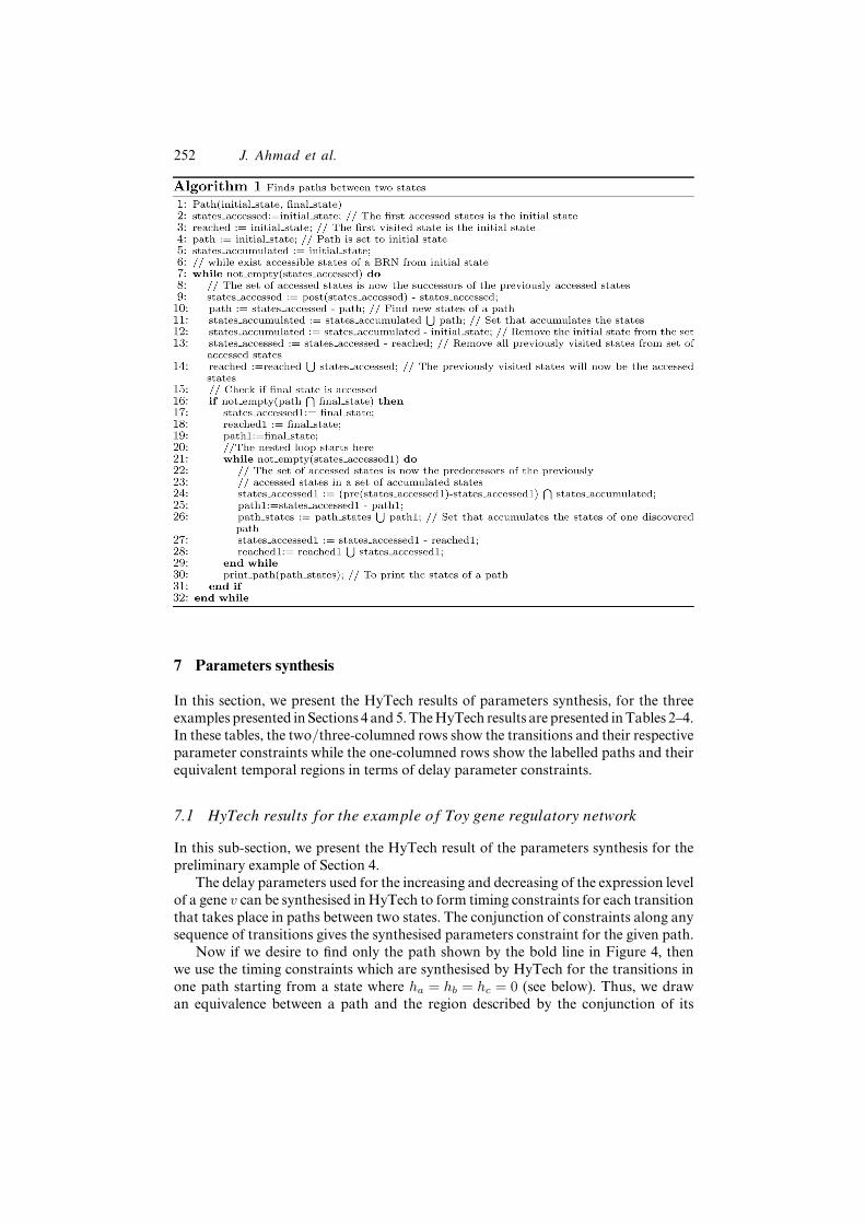
Algorithm1 is the pseudocodeof theHyTech implementation.pre andpostoperators,which are the classical predecessor and successor operators of hybrid systems analysis,return respectively the predecessors and successors of a state including the state itself.The difficulty of the algorithm lies in the fact that it converts the breadth-first search(induced by the post operator) into the depth-first search of a path. The algorithmconsists of two main loops. In the outer loop the algorithm exhaustively searchesthe final_state from the initial_state and accumulates the accessed states in aset named states_accumulated. When the algorithm finds the final_state thenit starts the nested loop and begins backward search from final_state and takesthe intersection of each accessed states with the set states_accumulated. If theintersection is not empty then the algorithm gives the intersection as a state ofthe path which is accumulated in a set path_states. Finally the algorithm invokes theprocedure print_path(path_states) to print the states of a path in proper order.

The dashed lines (A), (B) and (C) of Figure 9 represent the successive sets ofaccumulated states when the algorithm finds the final state f during the outer loop.The inner loop is used for backward search and the dashed arrow (D) shows this searchfor the first path. In Figure 9, the setA is equal to post(post(010)) and the set of pathstates is equal to post(post(010))

⋂pre(pre(111)).

Algorithm 1 finds the three paths between states (0,1,0) and (1,1,1) in the exampleof Figure 4.

252 J. Ahmad et al.

7 Parameters synthesis

In this section, we present the HyTech results of parameters synthesis, for the threeexamples presented in Sections 4 and 5. TheHyTech results are presented inTables 2–4.In these tables, the two/three-columned rows show the transitions and their respectiveparameter constraints while the one-columned rows show the labelled paths and theirequivalent temporal regions in terms of delay parameter constraints.

7.1 HyTech results for the example of Toy gene regulatory network

In this sub-section, we present the HyTech result of the parameters synthesis for thepreliminary example of Section 4.

The delay parameters used for the increasing and decreasing of the expression levelof a gene v can be synthesised in HyTech to form timing constraints for each transitionthat takes place in paths between two states. The conjunction of constraints along anysequence of transitions gives the synthesised parameters constraint for the given path.

Now if we desire to find only the path shown by the bold line in Figure 4, thenwe use the timing constraints which are synthesised by HyTech for the transitions inone path starting from a state where ha = hb = hc = 0 (see below). Thus, we drawan equivalence between a path and the region described by the conjunction of its


associated constraints. Table 2 shows the constraints synthesised by HyTech for theexample of Section 4.

Table 2 HyTech results of the delay constraints for the path shown by the bold linein Figure 4 (∧ means logical AND)

Transitions Constraints

010 → 011 d+c ≤ d−

b

011 → 001 d−b ≤ d+

a + d+c

001 → 101 d+a + d+

c ≤ d−b + d−

c

101 → 111 d+a + d+

b + d+c ≤ d−

b + d−c

010 → 011 → 001 → 101 → 111≡ (d+

c ≤ d−b ) ∧ (d−

b ≤ d+a + d+

c ) ∧ (d+a + d+

c ≤ d−b + d−

c ) ∧ (d+a + d+

b + d+c ≤ d−

b + d−c )

Table 3 HyTech results of the delay constraints for the paths shown in Figure 6

Transitions Constraints

0000 → 0001 d+u ≤ d+

x ∧ d+u ≤ d+

y

0001 → 0011 d+z + d+

u ≤ d+x ∧ d+

z + d+u ≤ d+

y

0011 → 1011 d+x ≤ d+

y

1011 → 2011 2d+x ≤ d+

y ∧ d+x ≤ d−

u

2011 → 2010 d+u ≤ d+

x + d−z

0000 → 0100 d+y ≤ d+

x ∧ d+y ≤ d+

u

0100 → 0200 2d+y ≤ d+

u

0100 → 0101 d+u ≥ 2d+

y

0101 → 0201 2d+y ≤ d+

z + d+u

0201 → 0200 2d+y + d−

u ≤ d+z + d+

u ∧ d−u ≤ d+

y

0201 → 0301 3d+y ≤ d+

z + d+u ∧ d+

y ≤ d−u

0301 → 0300 d−u ≤ d−

y

Path a: 0000 → 0001 → 0011 → 1011 → 2011 → 2010 → 2000≡ (d+

u ≤ d+x ∧ d+

u ≤ d+y ) ∧ (d+

z + d+u ≤ d+

x ∧ d+z + d+

u ≤ d+y ) ∧ (d+

x ≤ d+y )

∧(2d+x ≤ d+

y ∧ d+x ≤ d−

u ) ∧ (d+u ≤ d+

x + d−z )

Path b-1: 0000 → 0100 → 0200≡ (d+

y ≤ d+x ∧ d+

y ≤ d+u ) ∧ (2d+

y ≤ d+u )

Path b-2: 0000 → 0100 → 0101 → 0201 → 0200≡ (d+

y ≤ d+x ∧ d+

y ≤ d+u ) ∧ (d+

u ≥ 2d+y ) ∧ (2d+

y ≤ d+z + d+

u )∧(2d+

y + d−u ≤ d+

z + d+u ∧ d−

u ≤ d+y )

Path b-3: 0000 → 0100 → 0101 → 0201 → 0301 → 0300≡ (d+

y ≤ d+x ∧ d+

y ≤ d+u ) ∧ (d+

u ≥ 2d+y ) ∧ (3d+

y ≤ d+z + d+

u ∧ d+y ≤ d−

u )∧(2d+

y ≤ d+z + d+

u ) ∧ (d+u ≤ d−

y )

7.2 HyTech results for the example of Lambda phage

In this sub-section, we present the HyTech results of the parameter synthesis forthe example of lambda phage of Section 5.1. Here, we show paths leading to lyticand lysogenic states and their delay parameter constraints, representing equivalenttemporal regions. The equivalent regions give a choice among paths for lysogenesis

254 J. Ahmad et al.

and lysis (of Figure 5), as labelled in Table 3 by Path a and Paths b (b-1, b-2, b-3)respectively.

7.3 HyTech results for the T-cell activation and anergy system

In this sub-section, we present the HyTech results of the parameter synthesis for theexample of T-cell activation and anergy system of Section 5.2, along with the resultsgiven in Kaufman et al. (1999) for the same system, as shown here in Figure 10.We notice that HyTech gives the same results of delay constraints as manuallycalculated in Kaufman et al. (1999) and therefore this shows the usefulness of BRNmodelling alongwith theHyTech tool for the temporal analysis of regulatorynetworks.

Figure 10 State graph showing the total time to reach a given state, relative to time 0 in termsof time delays

Various timing dependent signalling properties presented in Kaufman et al. (1999,pp.3896–3898) are given below.

• Fast ligand dissociation. Path 1 is followed if ligand dissociation precedeskinase activation (d−

b < d+k ) and corresponds to what is observed for ‘null’ or

inactive ligands. Path 2 is followed if ligand dissociation is slower than kinaseactivation but faster than significant activation of the stimulatory and inhibitorypathways: d+

k < d−b < Min (d+

k + d+s ,d+

k + d+x ).


• Absence of costimulation. If d+x < d+

s and d+k + d+

x < d−b , path 3 will be

followed. Here, the receptor-associated kinases are activated but inhibitionprecedes significant signal transmission, so that there is no positive signalling.After ligand dissociation, the system ends up again in the unresponsive state andrestimulation in optimal conditions does not lead to cellular activation.

• Positive signalling. The general conditions for positive signalling are: d+s < d+

xand d+

k + d+s < d−

b . Positive signalling should be faster than significantinhibition, and the ligand residence time must exceed the time required foractivation of the kinases and signal transmission. These timing conditionscorrespond to paths 4–12 and account for signalling upon stimulation with anactivatory ligand in the presence of costimulation. Along paths 8–12(d−

b < d+k + d+

x ), the time length of the activation phase essentially isdetermined by the ligand residence time on the receptors, whereas alongpaths 4–7 (d+

k + d+x < d−

b ), it is mainly determined by the time lag betweenpositive signalling and inhibition.

After activation the systemwill end up in one of two stable steady states, correspondingeither to recovery of responsiveness (0000) or to anergy (0110). Independently of theprecise pathway that is followed, the necessary and sufficient conditions to reach eachof these two final states can be determined by using the tools of combinatorial logic.These additional conditions follow.

• For positive signalling with recovery of responsiveness:

(d−s > d−

k ) AND (d−b < d+

k + d+x + d−

s − d−k )

which means that the activatory phase will be followed by recovery ofimmunocompetence both if the ligand does not bind too strongly and positivesignalling does not decay before inactivation of the kinases.

This situation requires that the ligand residence time be in an optimal range andis related to a memory-type response.

• For positive signalling followed by anergy:

(d−s < d−

k ) OR (d+k + d+

x + d−s − d−

k < d−b )

which means that the activatory phase will be followed by anergy if either boththe positive signal decays rapidly or ligand dissociation is very slow. Thissituation corresponds to ‘activation-induced anergy’.

� End of (Kaufman et al., 1999) quotation.

One can notice that the constraints, as shown in bold faced, in the HyTech Table 4and in Kaufman et al. (1999) are exactly the same for all paths.

8 Cycles in BRN

The state graph of a BRN is not a simple tree like graph: it frequently contains cycles.It has been stated and then shown that cycles play a crucial role in the dynamics:

256 J. Ahmad et al.

Table 4 HyTech results for the delay constraints of the transitions of paths shown in Figure 8

Transitions Paths Constraints

1000 → 0000 1 d−b ≤ d+

k1000 → 1100 2–12 d+

k ≤ d−b

1100 → 0100 2 d−b ≤ d+

k + d+s ∧ d−

b≤ d+

k + d+x

1100 → 1110 3 d+x ≤ d+

s ∧ d+k + d+

x ≤ d−b

1100 → 1101 4–12 d+s ≤ d+

x ∧ d+k + d+

s ≤ d−b

1101 → 1111 4–7 d+k + d+

x ≤ d−b

1101 → 0101 8–12 d−b ≤ d+

k + d+x

1111 → 1110 4 d+k + d+

x + d−s ≤ d−

b

1111 → 0111 5–7 d−b ≤ d+

k + d+x + d−

s

0111 → 0110 5 d+k + d+

x + d−s ≤ d−

b + d−k

0111 → 0011 6–7 d−b + d−

k ≤ d+k + d+

x + d−s

0011 → 0001 6 d−b + d−

k + d−x ≤ d+

k + d+x + d−

s

0011 → 0010 7 d+k + d+

x + d−s ≤ d−

b + d−k + d−

x

0101 → 0111 8–10 d+k + d+

x ≤ d−b + d−

k ∧ d+k + d+

x

≤ d−b + d−

s

0101 → 0100 11 d−s ≤ d−

k ∧ d−b + d−

s ∧ d+k + d+

x

0101 → 0001 12 d−k ≤ d−

s ∧ d−b + d−

k ≤ d+k + d+

x

0111 → 0110 8 d−s ≤ d−

k0111 → 0011 9–10 d−

k ≤ d−s

0011 → 0001 9 d−k + d−

x ≤ d−s

0011 → 0010 10 d−s ≤ d−

k + d−x

Path 1: 1000 → 0000 ≡ d−b ≤ d+

k

Path 2: 1000 → 1100 → 0100 → 0110≡ (d+

k ≤ d−b ) ∧ (d−

b ≤ d+k + d+

s ∧ d−b ≤ d+

k + d+x )

Path 3: 1000 → 1100 → 1110 → 0110≡ (d+

k ≤ d−b ) ∧ (d+

x ≤ d+s ∧ d+

k + d+x ≤ d−

b )

Path 4: 1000 → 1100 → 1101 → 1111 → 1110 → 0110≡ (d+

k ≤ d−b ) ∧ (d+

s ≤ d+x ∧ d+

k + d+s ≤ d−

b ) ∧ (d+k + d+

x ≤ d−b ) ∧ (d+

k + d+x + d−

s ≤ d−b )

Path 5: 1000 → 1100 → 1101 → 1111 → 0111 → 0110≡ (d+

k ≤ d−b ) ∧ (d+

s ≤ d+x ∧ d+

k + d+s ≤ d−

b ) ∧ (d+k + d+

x ≤ d−b ) ∧ (d−

b ≤ d+k + d+

x + d−s )

∧(d+k + d+

x + d−s ≤ d−

b + d−k )

Path 6: 1000 → 1100 → 1101 → 1111 → 0111 → 0011 → 0001 → 0000≡ (d+

k ≤ d−b ) ∧ (d+

s ≤ d+x ∧ d+

k + d+s ≤ d−

b ) ∧ (d+k + d+

x ≤ d−b )

∧(d−b ≤ d+

k + d+x + d−

s ) ∧ (d−b + d−

k ≤ d+k + d+

x + d−s ) ∧ (d−

b + d−k + d−

x ≤ d+k + d+

x + d−s )

Path 7: 1000 → 1100 → 1101 → 1111 → 0111 → 0011 → 0010 → 0000≡ (d+

k ≤ d−b ) ∧ (d+

s ≤ d+x ∧ d+

k + d+s ≤ d−

b ) ∧ (d+k + d+

x ≤ d−b ) ∧ (d−

b ≤ d+k + d+

x + d−s )

∧(d−b + d−

k ≤ d+k + d+

x + d−s ) ∧ (d+

k + d+x + d−

s ≤ d−b + d−

k + d−x )

Path 8: 1000 → 1100 → 1101 → 0101 → 0111 → 0110≡ (d+

k ≤ d−b ) ∧ (d+

s ≤ d+x ∧ d+

k + d+s ≤ d−

b ) ∧ (d−b ≤ d+

k + d+x ) ∧ (d+

k + d+x ≤ d−

b + d−k )

∧(d+k + d+

x ≤ d−b + d−

s ) ∧ (d−s ≤ d−

k )

Path 9: 1000 → 1100 → 1101 → 0101 → 0111 → 0011 → 0001 → 0000≡ (d+

k ≤ d−b ) ∧ (d+

s ≤ d+x ∧ d+

k + d+s ≤ d−

b ) ∧ (d−b ≤ d+

k + d+x )

∧(d+k + d+

x ≤ d−b + d−

k ∧ d+k + d+

x ≤ d−b + d−

s ) ∧ (d−k ≤ d−

s ) ∧ (d−k + d−

x ≤ d−s )

Path 10: 1000 → 1100 → 1101 → 0101 → 0111 → 0011 → 0010 → 0000≡ (d+

k ≤ d−b ) ∧ (d+

s ≤ d+x ∧ d+

k + d+s ≤ d−

b ) ∧ (d−b ≤ d+

k + d+x )

∧(d+k + d+

x ≤ d−b + d−

k ∧ d+k + d+

x ≤ d−b + d−

s ) ∧ (d−k ≤ d−

s ) ∧ (d−s ≤ d−

k + d−x )

Path 11: 1000 → 1100 → 1101 → 0101 → 0100 → 0110≡ (d+

k ≤ d−b ) ∧ (d+

s ≤ d+x ∧ d+

k + d+s ≤ d−

b ) ∧ (d−b ≤ d+

k + d+x )

∧(d−s ≤ d−

k ∧ d−b + d−

s ∧ d+k + d+

x )

Path 12: 1000 → 1100 → 1101 → 0101 → 0001 → 0000≡ (d+

k ≤ d−b ) ∧ (d+

s ≤ d+x ∧ d+

k + d+s ≤ d−

b ) ∧ (d−b ≤ d+

k + d+x )

∧(d−k ≤ d−

s ∧ d−b + d−

k ≤ d+k + d+

x )


a positive circuit (resp. negative circuit) in the interaction graph is necessary to observemultistationarity (resp. homeostasis) (Thomas and Kaufman, 2001; Thomas et al.,1995; Cinquin and Demongeot, 2002; Soulé, 2003). For example, homeostasis isexpressed in the state graph by oscillatory behaviours (sustained or not), which areoften abstracted by cycles. Then it becomes important to analyse the entrance intosuch cycles. The delay constraints in Section 7 that can select a certain pathway can besynthesised in similar way to enter a cycle (Ahmad et al., 2006), as shown in Figure 3by bold arrows. But introducing delays in BRN modelling can make the cycle to bestable or unstable, depending on values of these delays (Bernot et al., 2007; Thomasand D’Ari, 1990). To remain stable in the cycle, some initial conditions in terms ofconstraints of delay parameters and clocks have to be synthesised such that some timedtrajectories from these initial conditions remain viable in a cycle. This is supposedto introduce the notion of invariance kernel Schneider (2004) that requires furthermodelling of BRN.

In real situations, however, the initial state is usually not in the cycle. It is thereforeimportant to analysewhich initial states can lead the system into the cycle, to determinethe constraints on the time delays which will effectively allow the system to enter thecycle and then to verify that these constraints are compatible with the conditions forremaining in the cycle.

Fixing the values for delays is also an issue in the context of time delays. If nothingis said about the time delays the whole graph remains indeed open, but if one assignsvalues to the delays (e.g., on the basis of biological data), only one well-definedtransition path will remain. Biological execution of such models are in fact subject tosome variations due to slight differences between delay parameters chosen by differentcells even in the homogeneous population (Thomas andD’Ari, 1990). Further analysiswith probabilistic models of these variations on delay parameters would be able toseparate different behaviours.

9 Conclusion

We propose in this paper a refinement of the concept of delays for BRN modelling.The introduction of delays allows one to distinguish paths from one state to anotherone. This refinement reintroduces time in the abstraction of R. Thomas, and this way isdifferent from the refinement of Batt et al. (2005) and Adélaïde and Sutre (2004) whichsplit the state space by partitioning the domains of the state space. The present workdescribes how the introduction of time can be helpful for modelling such networks,allowing the modeller to verify temporal properties. It is now important to confrontthis modelling with even more complex real systems where the underlying processesare not yet already known. Our experience in modelling in a multidisciplinary contextwill help to initiate biological modelling with delays.

In addition, we plane to deepen the following points:

• parameter synthesis: we have to check when a path is equivalent to an emptyregion and what this really means

• cycles: we have to look for invariance kernels in the state graph of BRN.

258 J. Ahmad et al.

Acknowledgements

We would like to acknowledge the many helpful suggestions of the anonymousreviewers on previous versions of this paper.

References

Adélaïde, M. and Sutre, G. (2004) ‘Parametric analysis and abstraction of geneticregulatory networks’, Proc. 2nd Workshop on Concurrent Models in Molecular Biology(BioCONCUR’04), London, UK, August, ser. Electronic Notes in Theor. Comp. Sci.,Elsevier, London, UK, (To appear).

Ahmad, J., Bernot, G., Comet, J-P., Lime, D. and Roux, O. (2006) ‘Hybrid modeling anddynamical analysis of gene regulatory networks with delays’, ComPlexUs, Vol. 3, No. 4,pp.231–251.

Alur, R., Courcoubetis, C., Halbwachs, N., Henzinger, T.A., Ho, P-H., Nicollin, X.,Olivero, A., Sifakis, J. and Yovine, S. (1995) ‘The algorithmic analysis of hybridsystems’, Theoretical Computer Science, Vol. 138, No. 1, pp.3–34, [Online], Available:citeseer.ist.psu.edu/alur95algorithmic.html

Alur, R., Courcoubetis, C., Henzinger, T.A. and Ho, P-H. (1992) ‘Hybrid automata: analgorithmic approach to the specification and verification of hybrid systems’, HybridSystems, pp.209–229, [Online], Available: citeseer.ist.psu.edu/alur92hybrid.html

Batt, G., Ropers, D., de Jong, H., Geiselmann, J., Page,M. and Schneider, D. (2005) ‘Qualitativeanalysis and verification of hybrid models of genetic regulatory networks: nutritional stressresponse in Escherichia coli’, in Morari, M. and Thiele, L. (Eds.): Eighth InternationalWorkshop on Hybrid Systems: Computation and Control, HSCC 2005, Ser. Lecture Notesin Computer Science, Vol. 3414, Springer, pp.134–150.

Bernot, G., Cassez, F., Comet, J-P., Delaplace, F., Müller, C., Roux, O. and Roux, O. (2007)‘Semantics of biological regulatory networks’, Proc. First Workshop on Concurrent Modelsin Molecular Biology (BioConcur 2003), Marseille, France, ser. Electronic Notes in Theor.Comp. Sci., Elsevier, Vol. 180, No. 3, pp.3–14.

Bernot, G., Comet, J-P., Richard, A. and Guespin, J. (2004) ‘Application of formal methods tobiological regulatory networks: extending Thomas’ asynchronous logical approach withtemporal logic’, Journal of Theoretical Biology, Vol. 229, No. 3, pp.339–347.

Cassez, F. and Larsen, K.G. (2000) ‘The impressive power of stopwatches’, CONCUR’00:Proceedings of the 11th International Conference on Concurrency Theory,Springer-Verlag, London, UK, pp.138–152.

Cinquin, O. and Demongeot, J. (2002) ‘Positive and negative feedback: striking a balancebetweennecessary antagonists, Journal ofTheoreticalBiology, Vol. 216,No. 2, pp.229–241.

de Jong, H. (2002) ‘Modeling and simulation of genetic regulatory systems: a literature review’,J. Comput. Biol., Vol. 9, No. 1, pp.67–103.

de Jong, H., Geiselmann, J., Batt, G., Hernandez, C. and Page,M. (2004) ‘Qualitative simulationof the initiation of sporulation in Bacillus subtilis’, Bulletin of Mathematical Biology,Vol. 66, No. 2, pp.261–299.

de Jong, H., Geiselmann, J., Hernandez, C. and Page, M. (2003) ‘Genetic network analyzer:qualitative simulation of genetic regulatory networks’, Bioinformatics, Vol. 19, No. 3,pp.336–344.

Devloo, V., Hansen, P. and Labbé,M. (2003) ‘Identification of all steady states in large networksby logical analysis’, Bull. Math. Biol., Vol. 65, No. 6, pp.1025–1051.


Henzinger, T-A., Ho, P-H. and Wong-Toi, H. (1997) ‘HYTECH: a model checker for hybridsystems’, International Journal on Software Tools for Technology Transfer, Vol. 1,Nos. 1–2, pp.110–122, [Online], Available: citeseer.ist.psu.edu/henzinger97hytech.html

Hill, C., Sawhill, B., Kauffman, S.A. and Glass, L. (1998) ‘Transition to chaos in models ofgenetic networks’, in StatisticalMechanics of Biocomplexity: Proceedings of theXV SitgesConference Held at Sitges, Barcelona, Spain, ser. Lecture Notes in Physics, Springer,Berlin/Heidelberg, Vol. 527, pp.261–274.

Kam, N., Cohen, I.R. and Harel, D. (2001) ‘The immune system as a reactive system: modelingT cell activation with statecharts’, Proceedings of the IEEE 2001 Symposia on HumanCentric Computing Languages and Environments (HCC’01), 05–07 September, p.15.

Kauffman, S. (2003) ‘Understanding genetic regulatory networks’, International Journal ofAstrobiology, Vol. 2, April, pp.131–139.

Kaufman, M., Andris, F. and Leo, O. (1999) ‘A logical analysis of T cell activation and anergy’,Proc. Natl. Acad. Sci. U.S.A., pp.3894–3899.

Schneider, G. (2004) ‘Computing invariance kernels of polygonal hybrid systems’, NordicJournal of Computing, Vol. 11, No. 2, pp.194–210.

Snoussi, E. (1989) ‘Qualitative dynamics of a piecewise-linear differential equations: a discretemapping approach’, DSS, Vol. 4, pp.189–207.

Snoussi, E. and Thomas, R. (1993) ‘Logical identification of all steady states : the concept offeedback loop characteristic states’, Bull. Math. Biol., Vol. 55, No. 5, pp.973–991.

Soulé, C. (2003) ‘Graphic requirements for multistationarity’, Complexus, Vol. 1, pp.123–133.

Thieffry, D. (1993) Modélisation des régulations Génétiques: une méthode logique, sonautomatisation et quelques applications, PhD Dissertation, Theoretical Biology Unit,Université Libre de Bruxelles, Belgium, 23 January.

Thomas, A.P., Henzinger, A., Kopke, P.W. and Varaiya, P. (1998) What’s Decidable aboutHybrid Automata, EECS Department, University of California, Berkeley, Tech. Rep.,[Online], Available: http://www.eecs.berkeley.edu/Pubs/TechRpts/1998/3418.html

Thomas, R. (1973) ‘Boolean formalization of genetic control circuits’, Journal of TheoreticalBiology, Vol. 425, pp.563–585.

Thomas, R. (1978) ‘Logical analysis of systems comprising feedback loops’, J. Theor. Biol.,Vol. 73, No. 4, pp.631–656.

Thomas, R. (1979) ‘Kinetic logic: a Boolean approach to the analysis of complex regulatorysystems’, Lecture Notes in Biomathematics, Vol. 29, p.507.

Thomas, R. (1991) ‘Regulatory networks seen as asynchronous automata: a logical description’,J. Theor. Biol., Vol. 153, pp.1–23.

Thomas, R. and D’Ari, R. (1990) Biological Feedback, CRC Press, Boca Raton, FL.

Thomas, R. and Kaufman, M. (2001) ‘Multistationarity, the basis of cell differentiation andmemory’, Chaos, Vol. 11, pp.180–195.

Thomas, R., Thieffry, D. and Kaufman, M. (1995) ‘Dynamical behaviour of biologicalregulatory networks-I’, Bull. Math. Biol., Vol. 57, No. 2, pp.9247–276.

Note

1In Figure 6, this cycle oscillates around a particular point named 0θ00. Theta generallycorresponds to a threshold above which (resp. below which) the concentration of Cro tends todecrease (resp. increase).

260 J. Ahmad et al.

Appendix A

In this appendix, we show the HyTech file for the example of Section 4. The HyTechfile consists of two parts: the hybrid automaton and the analysis commands.

A.1 Hybrid automaton

The following HyTech codes implement the stopwatch automaton of Figure 4.Here, the variables ha, hb and hc, represent the clocks associated to genes a, b and crespectively. These clocks evolve towards delay parameters dpa, dna, dpb, dnb, dpc anddnc during the activation and inhibition periods of their respective genes.


A.2 Analysis commands

The following HyTech codes implement Algorithm 1 of Section 6.

262 J. Ahmad et al.

Corresponding author Gilles Bernot, Jean-Paul ... -...

Documents

Transcript of Corresponding author Gilles Bernot, Jean-Paul ... -...