Core Maths C1

Revision Notes

November 2012

C1 14/04/2013 SDB 1

Core Maths C1

1 Algebra ................................................................................................................................ 3

Indices ...................................................................................................................................... 3 Rules of indices .................................................................................................................................................... 3

Surds......................................................................................................................................... 4 Simplifying surds ................................................................................................................................................. 4 Rationalising the denominator............................................................................................................................. 4

Quadratic functions.................................................................................................................. 4 Completing the square. ........................................................................................................................................ 4 Method 2 .............................................................................................................................................................. 5 Factorising quadratics .......................................................................................................................................... 6

Solving quadratic equations. .................................................................................................... 6 by factorising. ...................................................................................................................................................... 6 by completing the square ..................................................................................................................................... 6 by using the formula ............................................................................................................................................ 6 The discriminant b2 – 4ac .................................................................................................................................. 7 Miscellaneous quadratic equations...................................................................................................................... 7

Quadratic graphs ..................................................................................................................... 8 Simultaneous equations............................................................................................................ 9

Two linear equations ........................................................................................................................................... 9 One linear and one quadratic. .............................................................................................................................. 9

Inequalities ............................................................................................................................. 10 Linear inequalities ............................................................................................................................................. 10 Quadratic inequalities ........................................................................................................................................ 10

3 Coordinate geometry ....................................................................................................... 11

Distance between two points .................................................................................................. 11 Gradient ................................................................................................................................. 11 Equation of a line ................................................................................................................... 11 Parallel and perpendicular lines ........................................................................................... 11

4 Sequences and series ........................................................................................................ 12

Definition by a formula xn = f(n) ........................................................................................... 12 Definitions of the form xn+1 = f(xn) ........................................................................................ 12 Series and Σ notation ............................................................................................................. 12 Arithmetic series .................................................................................................................... 12

Proof of the formula for the sum of an arithmetic series .................................................................................. 13

5 Curve sketching ................................................................................................................ 14

Standard graphs ..................................................................................................................... 14 Transformations of graphs ..................................................................................................... 15

Translations ........................................................................................................................................................ 15 Stretches ............................................................................................................................................................. 15 Reflections in the x-axis .................................................................................................................................... 18 Reflections in the y–axis .................................................................................................................................... 18

C1 14/04/2013 SDB 2

6 Differentiation .................................................................................................................. 20

General result ........................................................................................................................ 20 Tangents and Normals ........................................................................................................... 20

Tangents ............................................................................................................................................................ 20 Normals ............................................................................................................................................................. 21

7 Integration ........................................................................................................................ 22

Indefinite integrals ................................................................................................................. 22 Finding the arbitrary constant ........................................................................................................................... 22

Index .......................................................................................................................................... 23

C1 14/04/2013 SDB 3

1 Algebra

Indices

Rules of indices am × an = am+n

am ÷ an = am–n

(am )n = amn

a0 = 1

a –n = na1

a an n1=

( )a a am

n mn nm

= =

Examples:

(i) 5 –3 × 54 = 5 –3 + 4 = 51 = 5.

7 –4 × 7 –2 = 7 –4 + –2 = 7 –4 – 2 = 7–6 = 176 .

(ii) 35 ÷ 3 –2 = 35 – –2 = 35 + 2 = 37.

9 –4 ÷ 96 = 9 –4 – 6 = 9–10 = 1910

11 –3 ÷ 11 –5 = 11 –3 – –5 = 11 –3 + 5 = 112 = 121

(iii) (6 –3)4 = 6 –3 × 4 = 6 –12 = 1612 .

(iv) 64 64 4 162

31

32

2= ⎛⎝⎜⎞⎠⎟ = =( )

(v) 125 1

125

23

23

−= since minus means turn upside down

= 152 , since 3 on bottom of fraction is cube root, 125 53 =

= 125

Example: (16a) ÷ (8b) = (24)a ÷ (23)b = 24a ÷ 23b = 24a – 3b.

Example: Find x if 92x = 27x + 1.

Solution: First notice that 9 = 32 and 27 = 33 and so

92x = 27x + 1 ⇒ (32)2x = (33)x + 1

⇒ 34x = 33x + 3

⇒ 4x = 3x + 3 ⇒ x = 3.

C1 14/04/2013 SDB 4

Surds A surd is a ‘nasty’ root – i.e. a root which is not rational

Thus 64 8 127

13 243 33 5= = − = −, , are rational and not surds

and 5 45 725 3, , − are irrational and are surds.

Simplifying surds Example: To simplify 50 we notice that 50 = 25 × 2 = 52 × 2

⇒ 50 = 25 2 25 2 5 2× = × = .

Example: To simplify 403 we notice that 40 = 8 × 5 = 23 × 5

⇒ 40 8 5 8 5 2 53 3 3 3 3= × = × = × .

Rationalising the denominator Rationalising means getting rid of surds.

We remember that multiplying (a + b) by (a – b) gives a2 – b2 which has the effect of squaring both a and b at the same time!!

Example: Rationalise the denominator of 2 3 53 5+−

.

Solution: 2 3 53 5+−

= 2 3 53 5+−

× ++

=+ + +

−

3 53 5

6 3 5 5 9 5 2 5

3 52 2

= 21 11 54

+ .

Quadratic functions A quadratic function is a function ax2 + bx + c, where a, b and c are constants and the highest power of x is 2.

Completing the square. Method 1

Rule: 1] The coefficient of x2 must be 1.

2] Halve the coefficient of x, square it then add it and subtract it.

Example: Complete the square in x2 – 6x + 7.

Solution: 1] The coefficient of x2 is already 1,

C1 14/04/2013 SDB 5

2] the coefficient of x is –6, halve it to give –3 then square to give 9 and add and subtract

x2 – 6x + 7 = x2 – 6x + 9 – 9 + 7

= (x – 3)2 – 2.

Notice that the minimum value of the expression is –2 when x = 3, since the minimum value of (x – 3)2 is 0.

Example: Complete the square in 3x2 + 24x – 5.

Solution: 1] The coefficient of x2 is not 1, so we must ‘fiddle’ it to make it 1, and then go on to step 2].

3x2 + 24x – 5 = 3(x2 + 8x) – 5

= 3(x2 + 8x + 42 – 42) – 5

= 3(x + 4)2 – 48 – 5

= 3(x + 4)2 – 53

Notice that the minimum value of the expression is –53 when x = –4, since the minimum value of (x + 4)2 is 0. Thus the vertex of the curve is at (–4, –53).

Method 2 Example: Re-write x2 – 12x + 7 in completed square form

Solution: We know that we need -6 (half the coefficient of x)

and that (x – 6)2 = x2 – 12x + 36

⇒ x2 – 12x + 7 = (x – 6)2 – 27

Notice that the minimum value of the expression is –27 when x = 6, since the minimum value of (x – 6)2 is 0. Thus the vertex of the curve is at (6, –27).

Example: Express 3x2 + 12x – 2 in completed square form.

Solution: The coefficient of x2 is not 1 so we must ‘take 3 out’

3x2 + 12x – 2 = 3(x2 + 4x) – 2

and we know that (x + 2)2 = x2 + 4x + 4, so x2 + 4x = (x + 2)2 – 4

⇒ 3x2 + 12x – 2 = 3(x2 + 4x) – 2 = 3[(x + 2)2 – 4] – 2

= 3(x + 2)2 – 14

Notice that the minimum value of the expression is –14 when x = –2, since the minimum value of (x – 2)2 is 0. Thus the vertex of the curve is at (–2, –14).

C1 14/04/2013 SDB 6

Factorising quadratics All the coefficients must be whole numbers (integers) then the factors will also have whole number coefficients.

Example: Factorise 10x2 + 11x – 6.

Solution: Looking at the 10x2 and the –6 we see that possible factors are

(10x ± 1), (10x ± 2), (10x ± 3), (10x ± 6), (5x ± 1), (5x ± 2), (5x ± 3), (5x ± 6), (2x ± 1), (2x ± 2), (2x ± 3), (2x ± 6), (x ± 1), (x ± 2), (x ± 3), (x ± 6),

Also the –6 tells us that the factors must have opposite signs, and by trial and error or common sense

10x2 + 11x – 6 = (2x + 3)(5x – 2).

Solving quadratic equations.

by factorising. Example: x2 – 5x + 6 = 0 ⇒ (x – 3)(x – 2) = 0

⇒ x – 3 = 0 or x – 2 = 0 ⇒ x = 3 or x = 2.

Example: x2 + 8x = 0 ⇒ x(x + 8) = 0 ⇒ x = 0 or x + 8 = 0 ⇒ x = 0 or x = –8

N.B. Do not divide through by x first: you will lose the root of x = 0.

by completing the square Example: x2 – 6x – 3 = 0

⇒ x2 – 6x = 3

and (x – 3)2 = x2 – 6x + 9

⇒ x2 – 6x + 9 = 3 + 9 ⇒ (x – 3)2 = 12

⇒ (x – 3) = ±√12 ⇒ x = 3 ± √12 = – 0.464 or 6.46.

by using the formula always try to factorise first.

ax2 + bx + c = 0 ⇒ x = − ± −b b ac

a

2 42

Example: 3x2 – x – 5 = 0 will not factorise, so we use the formula with

a = 3, b = –1, c = –5

⇒ x = − − ± − − × × −

×

1 1 4 3 52 3

2( ) ( )= –1.135 or +1.468

C1 14/04/2013 SDB 7

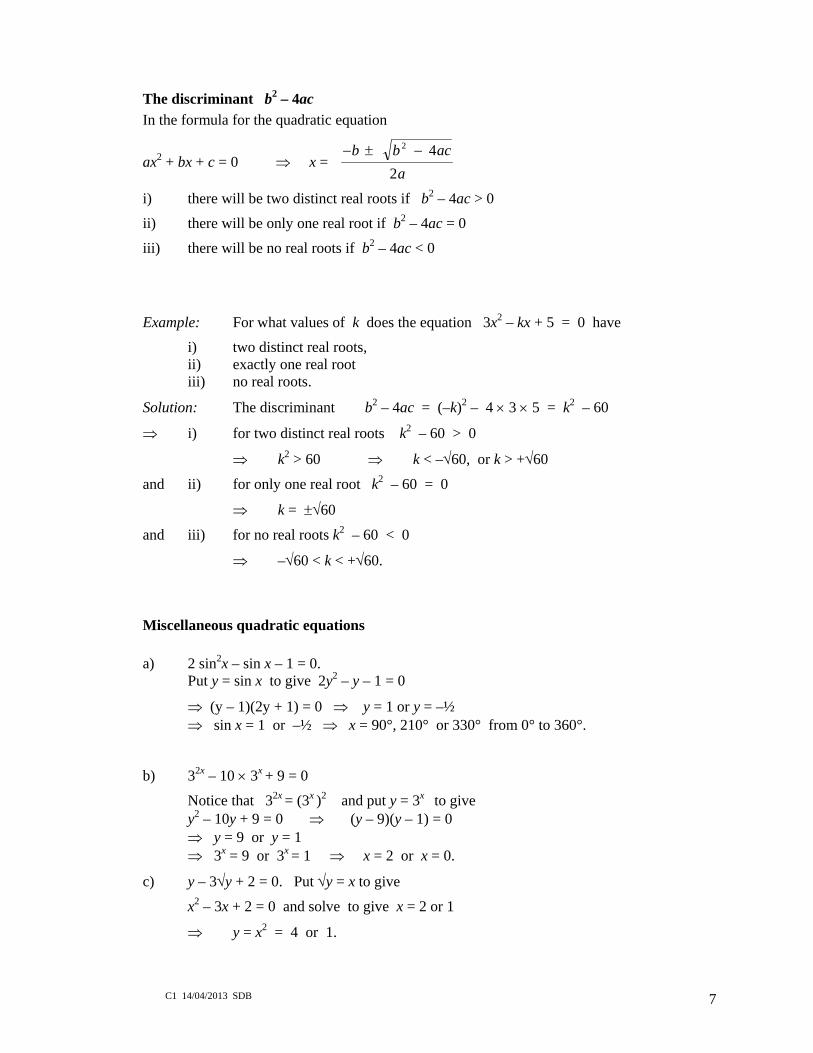
The discriminant b2 – 4ac In the formula for the quadratic equation

ax2 + bx + c = 0 ⇒ x = − ± −b b ac

a

2 42

i) there will be two distinct real roots if b2 – 4ac > 0

ii) there will be only one real root if b2 – 4ac = 0

iii) there will be no real roots if b2 – 4ac < 0

Example: For what values of k does the equation 3x2 – kx + 5 = 0 have

i) two distinct real roots, ii) exactly one real root iii) no real roots.

Solution: The discriminant b2 – 4ac = (–k)2 – 4 × 3 × 5 = k2 – 60

⇒ i) for two distinct real roots k2 – 60 > 0

⇒ k2 > 60 ⇒ k < –√60, or k > +√60

and ii) for only one real root k2 – 60 = 0

⇒ k = ±√60

and iii) for no real roots k2 – 60 < 0

⇒ –√60 < k < +√60.

Miscellaneous quadratic equations a) 2 sin2x – sin x – 1 = 0. Put y = sin x to give 2y2 – y – 1 = 0

⇒ (y – 1)(2y + 1) = 0 ⇒ y = 1 or y = –½ ⇒ sin x = 1 or –½ ⇒ x = 90°, 210° or 330° from 0° to 360°.

b) 32x – 10 × 3x + 9 = 0

Notice that 32x = (3x )2 and put y = 3x to give y2 – 10y + 9 = 0 ⇒ (y – 9)(y – 1) = 0 ⇒ y = 9 or y = 1 ⇒ 3x = 9 or 3x = 1 ⇒ x = 2 or x = 0.

c) y – 3√y + 2 = 0. Put √y = x to give

x2 – 3x + 2 = 0 and solve to give x = 2 or 1

⇒ y = x2 = 4 or 1.

C1 14/04/2013 SDB 8

Quadratic graphs a) If a > 0 the parabola will be ‘the right way up’

i) if b2 – 4ac > 0 the curve will meet the x-axis in two points.

ii) if b2 – 4ac = 0 the curve will meet the x-axis in only one point (it will touch the axis)

iii) if b2 – 4ac < 0 the curve will not meet the x-axis.

b) a) If a < 0 the parabola will be ‘the wrong way up’

i) if b2 – 4ac > 0 the curve will meet the x-axis in two points.

ii) if b2 – 4ac = 0 the curve will meet the x-axis in only one point (it will touch the axis)

iii) if b2 – 4ac < 0 the curve will not meet the x-axis.

Note: When sketching the curve of a quadratic function you should always show the value on the y-axis and

if you have factorised you should show the values where it meets the x-axis,

if you have completed the square you should give the co-ordinates of the vertex.

C1 14/04/2013 SDB 9

Simultaneous equations

Two linear equations Example: Solve 3x – 2y = 4 and 4x + 7y = 15.

Solution: Make the coefficients of x (or y) equal then add or subtract the equations to eliminate x (or y).

Here 4 times the first equation gives 12x – 8y = 16 and 3 times the second equation gives 12x + 21y = 45

Subtracting gives –29y = –29 ⇒ y = 1

Put y = 1 in equation one ⇒ 3x = 4 + 2y = 4 + 2 ⇒ x = 2

Check in equation two: L.H.S. = 4 × 2 + 7 × 1 = 15 = R.H.S.

One linear and one quadratic. Find x (or y) from the Linear equation and substitute in the Quadratic equation.

Example: Solve x – 2y = 3, x2 – 2y2 – 3y = 5

Solution: From first equation x = 2y + 3

Substitute in second ⇒ (2y + 3)2 – 2y2 – 3y = 5

⇒ 4y2 + 12y + 9 – 2y2 – 3y = 5

⇒ 2y2 + 9y + 4 = 0 ⇒ (2y + 1)(y + 4) = 0

⇒ y = –½ or y = –4

⇒ x = 2 or x = –5 from the linear equation.

Check in quadratic for x = 2, y = –½

L.H.S. = 22 – 2(–½)2 – 3(–½) = 5 = R.H.S.

and for x = –5, y = –4

L.H.S. = (–5)2 – 2(–4)2 – 3(–4) = 25 – 32 + 12 = 5 = R.H.S.

C1 14/04/2013 SDB 10

Inequalities

Linear inequalities Solving algebraic inequalities is just like solving equations, add, subtract, multiply or divide the same number to, from, etc. BOTH SIDES

EXCEPT - if you multiply or divide both sides by a NEGATIVE number then you must TURN THE INEQUALITY SIGN ROUND.

Example: Solve 3 + 2x < 8 + 4x

Solution: sub 3 from B.S. ⇒ 2x < 5 + 4x sub 4x from B.S. ⇒ -2x < 5 divide B.S. by -2 and turn the inequality sign round ⇒ x > - 2.5.

Example: Solve x2 > 16

Solution: We must be careful here since the square of a negative number is positive giving the full range of solutions as

⇒ x < -4 or x > +4.

Quadratic inequalities Always sketch a graph and find where the curve meets the x-axis

Example: Find the values of x which satisfy

3x2 – 5x – 2 ≥ 0.

Solution: 3x2 – 5x – 2 = 0

⇒ (3x + 1)(x – 2) = 0

⇒ x = –1/3 or 2

We want the part of the curve which is above or on the x-axis

⇒ x ≤ –1/3 or x ≥ 2

-5

x

y

C1 14/04/2013 SDB 11

3 Coordinate geometry

Distance between two points Distance between P (a1, b1) and Q (a2, b2) is ( ) ( )a a b b1 2

21 2

2− + −

Gradient

Gradient of PQ is mb ba a

=−−

2 1

2 1

Equation of a line Equation of the line PQ, above, is y = mx + c and use a point to find c

or the equation of the line with gradient m through the point (x1, y1) is

y – y1 = m(x – x1)

or the equation of the line through the points (x1, y1) and (x2, y2) is

12

12

1

1

xxyy

xxyy

−−

=−−

(you do not need to know this one!!)

Parallel and perpendicular lines Two lines are parallel if they have the same gradient and they are perpendicular if the product of their gradients is –1.

Example: Find the equation of the line through (4½, 1) and perpendicular to the line joining the points A (3, 7) and B (6, -5).

Solution: Gradient of AB is 46357

−=−−−

⇒ gradient of line perpendicular to AB is ¼ , (product of perpendicular gradients is –1)

so we want the line through (4½, 1) with gradient ¼ .

Using y – y1 = m(x – x1) ⇒ y – 1 = ¼ (x – 4½)

⇒ 4y – x = - ½ or – 2x + 8y + 1 = 0.

C1 14/04/2013 SDB 12

4 Sequences and series A sequence is any list of numbers.

Definition by a formula xn = f(n) Example: The definition xn = 3n2 – 5 gives

x1 = 3 × 12 – 5 = –2, x2 = 3 × 22 – 5 = 7, x3 = 3 × 32 – 5 = 22, … .

Definitions of the form xn+1 = f(xn) These have two parts:– (i) a starting value (or values)

(ii) a method of obtaining each term from the one(s) before.

Examples: (i) The definition x1 = 3 and xn = 3xn –1 + 2

defines the sequence 3, 11, 35, 107, . . .

(ii) The definition x1 = 1, x2 = 1, xn = xn –1 + xn –2

defines the sequence 1, 1, 2, 3, 5, 8, 13, 21, 34, 65, . . . .

This is the Fibonacci sequence.

Series and Σ notation A series is the sum of the first so many terms of a sequence.

For a sequence whose nth term is xn = 2n +3 the sum of the first n terms is a series

Sn = x1 + x2 + x3 + x4 . . . + xn = 5 + 7 + 9 + 11 + . . . + (2n + 3)

This is written in Σ notation as Sn = ∑=

n

iix

1 = ( )2 3

1

ii

n

+=∑ and is a finite series of n terms.

An infinite series has an infinite number of terms S∞ = ∑∞

=1iix .

Arithmetic series An arithmetic series is a series in which each term is a constant amount bigger (or smaller) than the previous term: this constant amount is called the common difference.

Examples: 3, 7, 11, 15, 19, 23, . . . . with common difference 4

28, 25, 22, 19, 16, 13, . . . with common difference –3.

Generally an arithmetic series can be written as

Sn = a + (a + d) + (a + 2d) + (a + 3d) + (a + 4d) + . . . upto n terms,

where the first term is a and the common difference is d.

The nth term xn = a + (n – 1)d

The sum of the first n terms of the above arithmetic series is

C1 14/04/2013 SDB 13

Sn = ( )n a n d2

2 1+ −( ) , or Sn = ( )n a L2

+ where L is the last term.

Example: Find the nth term and the sum of the first 100 terms of the arithmetic series with 3rd term 5 and 7th term 17.

Solution: x7 = x3 + 4 × d

⇒ 17 = 5 + 4 × d ⇒ d = 3

⇒ x1 = x3 – 2 × d ⇒ x1 = 5 – 6 = –1

⇒ nth term xn = a + (n – 1)d = –1 + 3(n – 1)

and ⇒ S100 = 100/2 × (2 × –1 + (100 – 1) × 3) = 14750.

Proof of the formula for the sum of an arithmetic series You must know this proof.

First write down the general series and then write it down in reverse order

Sn = a + (a + d) + (a + 2d) + ….. + (a + (n – 2)d) + (a + (n – 1)d

⇒ Sn = (a + (n – 1)d + (a + (n – 2)d) + (a + (n – 3)d) + … + (a + d) + a ADD

⇒ 2 × Sn = (2a + (n – 1)d) + (2a + (n – 1)d) + (2a + (n – 1)d) + … (2a + (n – 1)d) + (2a + (n – 1)d)

⇒ 2 × Sn = n(2a + (n – 1)d)

⇒ Sn = n/2 × (2a + (n – 1)d),

Which can be written as Sn = n/2 × (a + a + (n – 1)d) = n/2 × (a + L), where L is the last term.

C1 14/04/2013 SDB 14

5 Curve sketching

Standard graphs

-4 -3 -2 -1 1 2 3 4 5

-3

-2

-1

1

2

3

x

y

-4 -3 -2 -1 1 2 3 4 5

-3

-2

-1

1

2

3

x

y

-4 -3 -2 -1 1 2 3 4 5

-3

-2

-1

1

2

3

x

y

-4 -3 -2 -1 1 2 3 4 5

-3

-2

-1

1

2

3

x

y

-4 -3 -2 -1 1 2 3 4 5

-3

-2

-1

1

2

3

x

y

-4 -3 -2 -1 1 2 3 4 5

-3

-2

-1

1

2

3

x

y

-4 -3 -2 -1 1 2 3 4 5

-3

-2

-1

1

2

3

x

y

-4 -3 -2 -1 1 2 3 4 5 6 7 8 9 1

10

20

x

y

y =3x2 is like y = x2 but steeper: similarly for y = 5x3 and y = 7/x, etc.

y = (x – a)(x – b)(x – c) y = (x – a)2(x – b)

y = (a – x)(x – b)(x – c) y = (a – x)(x – b)2

y = x y = x2

y = x3 y = 1/x y = 1/x2

y = √x The exponential curve y =2x

y = -x

a c b >x a b >x

>xa b c >xa b

C1 14/04/2013 SDB 15

Transformations of graphs

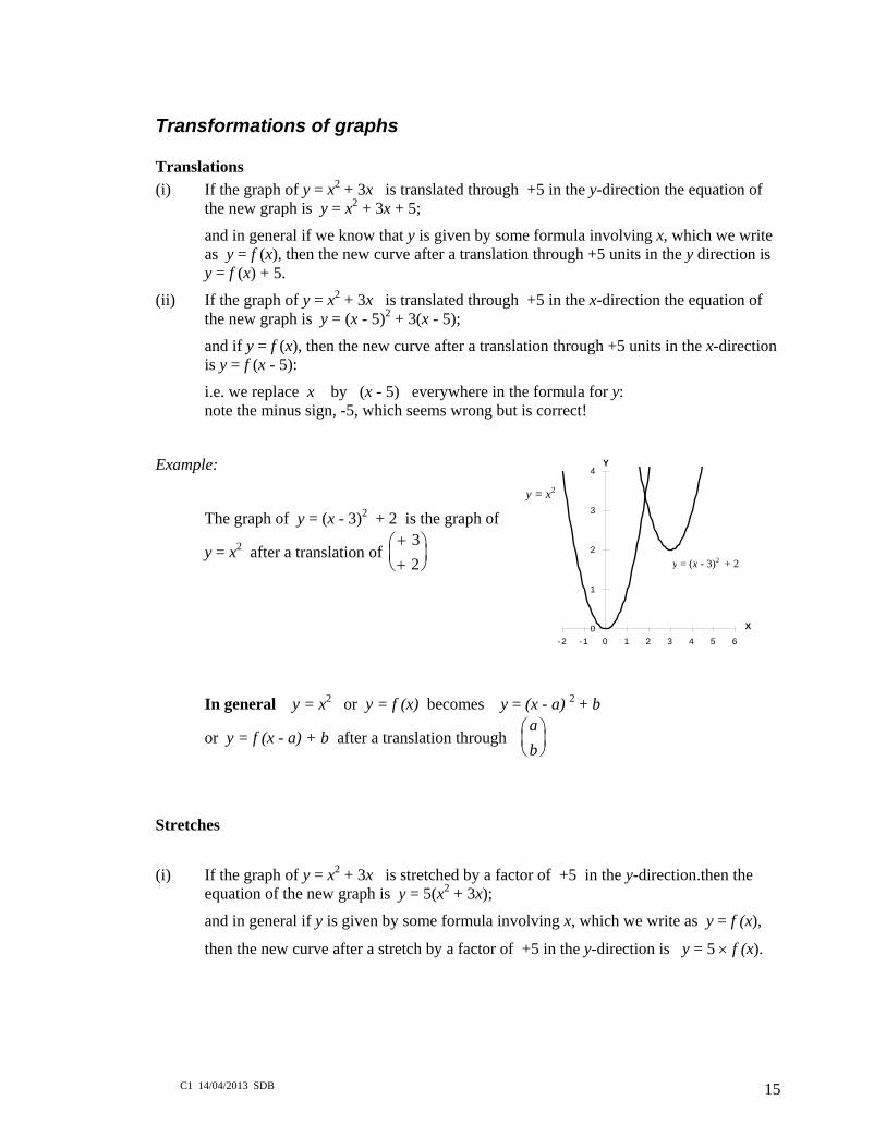
Translations (i) If the graph of y = x2 + 3x is translated through +5 in the y-direction the equation of

the new graph is y = x2 + 3x + 5;

and in general if we know that y is given by some formula involving x, which we write as y = f (x), then the new curve after a translation through +5 units in the y direction is y = f (x) + 5.

(ii) If the graph of y = x2 + 3x is translated through +5 in the x-direction the equation of the new graph is y = (x - 5)2 + 3(x - 5);

and if y = f (x), then the new curve after a translation through +5 units in the x-direction is y = f (x - 5):

i.e. we replace x by (x - 5) everywhere in the formula for y: note the minus sign, -5, which seems wrong but is correct!

Example:

The graph of y = (x - 3)2 + 2 is the graph of

y = x2 after a translation of ++⎛⎝⎜

⎞⎠⎟

32

In general y = x2 or y = f (x) becomes y = (x - a) 2 + b

or y = f (x - a) + b after a translation through ab⎛⎝⎜⎞⎠⎟

Stretches

(i) If the graph of y = x2 + 3x is stretched by a factor of +5 in the y-direction.then the equation of the new graph is y = 5(x2 + 3x);

and in general if y is given by some formula involving x, which we write as y = f (x),

then the new curve after a stretch by a factor of +5 in the y-direction is y = 5 × f (x).

0

1

2

3

4

-2 -1 0 1 2 3 4 5 6

X

Y

y = (x - 3)2 + 2

y = x2

C1 14/04/2013 SDB 16

Example:

The graph of y = x2 - 2 becomes

y = 3(x2 - 2) after a stretch of factor 3 in the y-direction

In general y = x2 or y = f (x) becomes y = ax2 or y = af (x) after a stretch in the y-direction of factor a.

(ii) If the graph of y = x2 + 3x is stretched by a factor of +3 in the x-direction then the

equation of the new graph is y = ⎟⎠⎞

⎜⎝⎛+⎟

⎠⎞

⎜⎝⎛

33

3

2 xx

and in general if y is given by some formula involving x, which we write as y = f (x),

then the new curve after a a stretch by a factor of +3 in the x-direction is y = f x3

⎛⎝⎜

⎞⎠⎟

i.e. we replace x by x3

everywhere in the formula for y.

-6

-5

-4

-3

-2

-1

0

1

2

3

4

-4 -3 -2 -1 0 1 2 3 4

X

Y

y = x2 - 2

y = 3(x2 - 2)

C1 14/04/2013 SDB 17

Example:

In this example the graph of y = x3 – 4 x has been stretched by a factor of 2 in the x-direction to form a new graph with equation

y x x= ⎛⎝⎜

⎞⎠⎟− ⎛

⎝⎜⎞⎠⎟2

42

3

(iii) Note that to stretch by a factor of ¼ in the x-direction we replace x by x x1

4

4= so

that y = f (x) becomes y = f (4x)

Example:

In this example the graph of y = x3 - 9 x

has been stretched by a factor of 13

in the

x-direction to form a new graph with equation

( ) ( )33 9 3y x x= − = 27x3 – 27x,

The new equation is formed by replacing x

by x x1

3

3= in the original equation.

-8-7-6-5-4-3-2-1012345678

-5 -4 -3 -2 -1 0 1 2 3 4 5

X

Y

-15-13-11-9-7-5-3-113579

111315

-5 -4 -3 -2 -1 0 1 2 3 4 5

X

Y

y = x3 – 4x

y = x3 - 9 x

( ) ( )33 9 3y x x= −

y x x= ⎛⎝⎜

⎞⎠⎟− ⎛

⎝⎜⎞⎠⎟2

42

3

C1 14/04/2013 SDB 18

Reflections in the x-axis When reflecting in the x-axis all the positive y-coordinates become negative and vice versa and so the image of y = f (x) after reflection in the x-axis is y = – f (x).

Example: The image of y = x2 + 2x – 1 after reflection in the x-axis is

y = –f (x)

= –(x2 + 2x – 1)

= –x2 – 2x + 1

Reflections in the y–axis When reflecting in the y-axis

the y-coordinate for x = +3 becomes the y-coordinate for x = –3 and the y-coordinate for x = –2 becomes the y-coordinate for x = +2.

Thus the equation of the new graph is found by replacing x by –x and the image of y = f (x) after reflection in the y–axis is y = f (–x).

Example: The image of

y = x2 + 2x – 1

after reflection in the y-axis is

y = (–x)2 + 2(–x) – 1 = x2 – 2x – 1

-4 -2 2 4

-2

2

x

y

y = – x2 – 2x + 1.

y = x2 + 2x – 1.

-4 -2 2 4

-2

2

x

yy = x2 + 2x – 1 y = x2 – 2x – 1

C1 14/04/2013 SDB 19

Old equation

Transformation New equation

y = f (x) Translation through

ab⎛⎝⎜⎞⎠⎟

y = f (x - a) + b

y = f (x)

Stretch with factor a in the y-direction.

y = a × f (x)

y = f (x)

Stretch with factor a in the x-direction. y = f x

a⎛⎝⎜

⎞⎠⎟

y = f (x) Stretch with factor 1

a

in the x-direction.

y = ( )f ax

y = f (x)

Reflection in the x-axis y = - f (x)

y = f (x)

Reflection in the y-axis y = f (-x)

C1 14/04/2013 SDB 20

6 Differentiation

General result Differentiating is finding the gradient of the curve.

y = xn ⇒ 1−= nnxdxdy , or f (x) = xn ⇒ f ′(x) = nxn–1

Examples:

a) y = 3x2 – 7x + 4 dxdy = 6x – 7

b) f (x) = 7√x = 21

7x x

xxf2

77)( 21

21 =×=′

−

c) y = 33 88 −= x

x 4

4 2438x

xdxdy −

=×= −−

d) f (x) = (2x + 1)(x – 3) multiply out first = 2x2 – 5x – 3 54)( −=′ xxf

e) y = 5

27 43x

xx − split up first

= 325

2

5

7

4343 −−=− xxxx

xx 4

4 126126x

xxxdxdy

+=−−= −

Tangents and Normals

Tangents Example:

Find the equation of the tangent to y = 3x2 – 7x + 5 at the point where x = 2.

Solution:

We first find the gradient when x = 2.

y = 3x2 – 7x + 5 ⇒ dydx

= 6x – 7 and when x = 2, dydx

= 6 × 2 – 7 = 5.

so the gradient when x = 2 is 5. The equation is of the form y = mx + c where m is the gradient so we have

y = 5x + c.

To find c we must find a point on the line, namely the point on the curve when x = 2.

When x = 2 the y – value on the curve is 3 2 7 2 5 32× − × + = ,

i.e. when x = 2, y = 3.

Substituting these values in y = 5x + c we get 3 = 5 × 2 + c ⇒ c = –7

⇒ the equation of the tangent is y = 5x – 7.

C1 14/04/2013 SDB 21

Normals (The normal to a curve is the line at 90o to the tangent at that point).

We first remember that if two lines with gradients m1 and m2 are perpendicular

then m1 × m2 = –1.

Example:

Find the equation of the normal to the curve y xx

= +2 at the point where x = 2.

Solution: We first find the gradient of the tangent when x = 2.

y = x + 2x–1 ⇒ dydx

= 1 – 2x–2 = 1 – 22x

⇒ when x = 2 gradient of the tangent is m1 = 1 – 24

= ½ .

If gradient of the normal is m2 then m1 × m2 = –1 ⇒ ½ × m2 = –1 ⇒ m2 = –2 Thus the equation of the normal must be of the form y = –2x + c.

From the equation y xx

= +2 the value of y when x = 2 is y = 2 + 2

23=

Substituting x = 2 and y = 3 in the equation of the normal y = –2x + c we have

3 = –2 × 2 + c ⇒ c = 7

⇒ equation of the normal is y = –2x + 7.

C1 14/04/2013 SDB 22

7 Integration

Indefinite integrals

∫ ++

=+

Cnxdxx

nn

1

1

provided that n ≠ –1

N.B. NEVER FORGET THE ARBITRARY CONSTANT + C.

Examples:

a) ∫ ∫ −= dxxdxx

66 3

43

4

= Cx

Cx+

−=+

−×

−

5

5

154

534

b) ∫ ∫ −+=+− dxxxdxxx 23)1)(23( 2 multiply out first = x3 + ½ x2 – 2x + C.

c) ∫ ∫ −+=+ dxxxdxx

xx 345

29

55 split up first

= 5 2 5

2

555 2 5 2x x xC C

x

−

+ × + = − +−

Finding the arbitrary constant If you know the derivative (gradient) function and a point on the curve you can find C.

Example: Solve 53 2 −= xdxdy , given that y = 4 when x = 2.

Solution: y = ∫ − dxx 53 2 = x3 – 5x + C but y = 4 when x = 2

⇒ 4 = 23 – 5 × 2 + C ⇒ C = 6

⇒ y = x3 – 5x + 6.

C1 14/04/2013 SDB 23

Index Differentiation, 20 Distance between two points, 11 Equation of a line, 11 Gradient, 11 Graphs

Reflections, 18 Standard graphs, 14 Stretches, 15 Translations, 15

Indices, 3 Inequalities

linear inequalities, 10 quadratic inequalities, 10

Integrals finding arbitrary constant, 22 indefinite, 22

Normals, 21 Parallel and perpendicular lines, 11

Quadratic equations b2 – 4ac, 7 completing the square, 6 factorising, 6 formula, 6 miscellaneous, 7

Quadratic functions, 4 completing the square, 4 factorising, 6 vertex of curve, 5

Quadratic graphs, 8 Series

Arithmetic, 12 Arithmetic, proof of sum, 13 Sigma notation, 12

Simultaneous equations one linear equations and one quadratic, 9 two linear equations, 9

Surds, 4 rationalising the denominator, 4

Tangents, 20