Copyright: IPGRI and Cornell University, 2003 Measures 1 · slide, Ind 1, Ind 2, … may represent,...

1

Copyright: IPGRI and Cornell University, 2003 Measures 1

Genetic diversity analysis with

molecular marker data:

Learning module

Measures of genetic

diversity

2


Basic genetic diversity analysisTypes of variablesQuantifying genetic diversity:

• Measuring intrapopulation genetic diversity• Measuring interpopulation genetic diversity

Quantifying genetic relationships:• Diversity and differentiation at the nucleotide level• Genetic distance

Displaying relationships:• Classification or clustering• Ordination

Appendices

Contents

3


1. Description of variation within and between populations, regions, etc.

2. Assessment of relationships among individuals, populations, regions, etc.

3. Expression of relationships between results obtained from different sets of characters

Ind5

Ind3

Ind6

Ind4

Ind2

Ind1

Basic genetic diversity analysis

00.460.370.560.560.3306

00.280.370.430.3205

00.500.260.4704

00.330.3303

00.5602

001

060504030201

Market 000111

110101

001100

110001

010110

110001

101101

data

Individuals

Most of the genetic diversity analysis that we might want to do will involve the following steps:

1. Describing the diversity. This may be done within a population or between populations. It may also extend to larger units such as areas and regions.

2. Calculating the relationships between the units analysed in step one. This entails calculating the distances (geometric or genetic) among all pairs of subjects in the study.

3. Expressing these relationships with any classification and/or ordination

method at hand. Some of these methods will permit comparing the results of our molecular study with other types of data (e.g. geographical). In the slide, Ind1, Ind2, … may represent, instead of individuals, populations or regions.

4


Qualitative. These refer to characters or qualities, and are either binary or categorical:

• Binary, taking only two values: present (1) or absent (0)

• Categorical, taking a value among many possibilities, and are either ordinal or nominal:

Ordinal: categories that have an orderNominal: categories that are unrelated

Quantitative. These are numerical and are either continuous or discrete:

• Continuous, taking a value within a given range• Discrete, taking whole or decimal numbers

Types of variable

Examples of qualitative variables:• Binary: e.g. leaf hairiness: present (1), absent (0)• Categorical:

Ordinal: e.g. stalk hairs: rare (1), common (2), abundant (3) orpetiole length: short (1), medium (2), long (3)Nominal: e.g. petal colour: yellow (1), red (2), white (3), purple (4)

Examples of quantitative variables:• Continuous: e.g. root weight (g); leaf length (cm) • Discrete: e.g. number of stamens: 2, 3, 4, ...

number of fruits: 1, 2, 3, …

Categorical variables can be converted to binary variables, but with limitations because, as we will see later, some similarity coefficients give a weight to the category of a character and this may bias against other characters being evaluated. That is, the more categories a variable has, the more weight it has when combined with other binary or categorical variables with few categories.

An example of converting a categorial variable into a binary one:Petiole length: short (1), medium (2), long (3)

Short: present (1), absent (0)Medium: present (1), absent (0)Long: present (1), absent (0)

Quantitative variables can also be converted to binary variables, for example: From 0 to 3 fruits: present (1), absent (0)From 4 to 7 fruits: present (1), absent (0), ...

5


Quantifying genetic diversity: measuringintrapopulation genetic diversity

Based on the number of variants• Polymorphism or rate of polymorphism (Pj)• Proportion of polymorphic loci• Richness of allelic variants (A)• Average number of alleles per locus

Based on the frequency of variants• Effective number of alleles (Ae)• Average expected heterozygosity (He; Nei’s genetic

diversity)

6


A gene is defined as polymorphic if the frequency of one of its alleles is less than or equal to 0.95 or 0.99

Pj = q 0.95 or Pj = q 0.99

Polymorphism or rate of polymorphism (Pj)

Where,Pj = rate of polymorphismq = allele frequency

• This measure provides criteria to demonstrate that a gene is showing variation.

• Its calculation is through direct observation of whether the definition is fulfilled.

• It can be used with codominant markers and, very restrictively, with dominant markers. This is because the estimate based on dominant markers would be biased below the real number.

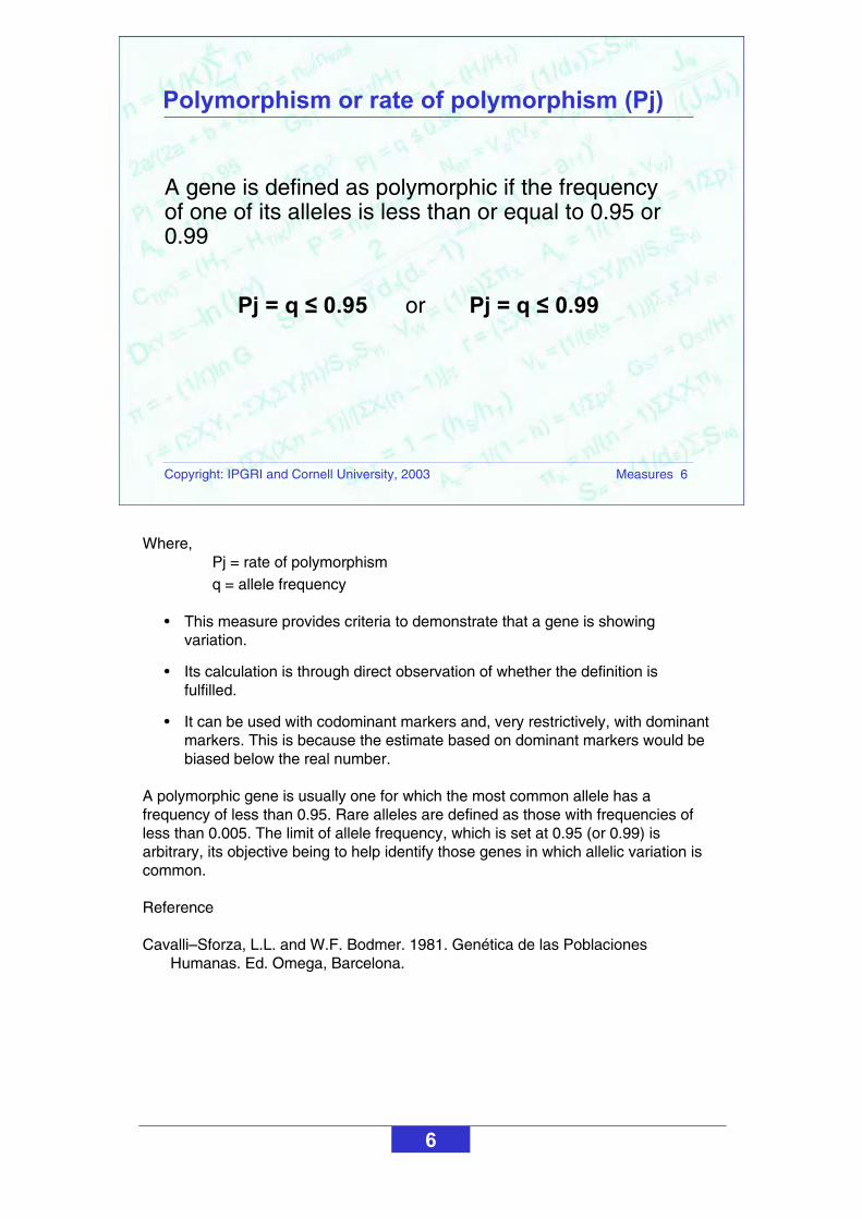
A polymorphic gene is usually one for which the most common allele has a frequency of less than 0.95. Rare alleles are defined as those with frequencies of less than 0.005. The limit of allele frequency, which is set at 0.95 (or 0.99) is arbitrary, its objective being to help identify those genes in which allelic variation is common.

Reference

Cavalli–Sforza, L.L. and W.F. Bodmer. 1981. Genética de las Poblaciones Humanas. Ed. Omega, Barcelona.

7


This the number of polymorphic loci divided by the total number of loci (polymorphic and monomorphic), that is:

P = npj/ntotal

Proportion of polymorphic loci

Where,P = proportion of polymorphic locinpj = number of polymorphic locintotal = total number of loci

• It expresses the percentage of variable loci in a population.

• Its calculation is based on directly counting polymorphic and total loci.

• It can be used with codominant markers and, very restrictively, with dominant markers (see previous slide for explanation).

8


Refers to the number of variants in a sample

The measure of diversity is (A - 1) variants because, within a monomorphic population, the degree of diversity is zero (A - 1 = 0)

Richness of allelic variants (A)

• For a given gene in a sample, this measure tells how many allelic variants can be found.

• It is sensitive to sample size.

• Although the distribution of alleles does not matter, the maximum number of alleles does.

• The measure can only be applied with codominant markers.

9


K

1i

in1/Kn

Average number of alleles per locus

It is the sum of all detected alleles in all loci, divided by the total number of loci

Where,K = the number of loci ni = the number of alleles detected per locus

• This measure provides complementary information to that of polymorphism.

• It requires only counting the number of alleles per locus and then calculating the average.

• It is best applied with codominant markers, because dominant markers do not permit the detection of all alleles.

10


Effective number of alleles (Ae)

It is the number of alleles that can be present in a population

Ae = 1/(1 – h) = 1/ pi2

Where,pi = frequency of the ith allele in a locus

h = 1 – pi2 = heterozygosity in a locus

• The measure tells about the number of alleles that would be expected in a locus in each population.

• It is calculated by inverting the measure of homozygosity in a locus.

• It can be used with codominant marker data.

• Its calculation may be affected by sample size.

This measure of diversity may be informative for establishing collecting strategies. For example, we estimate it in a given sample. We then verify it in a different sample or the entire collection. If the figure obtained the second time is less than the first estimated number, this could mean that our collecting strategy needs revising.

11


0.30Frequency of allele 4

2.00

0.50

0.50

0.50

2

A1 A2

A2 A2

A2 A2

A1 A1

A1 A1

Population 2

3.33

0.70

0.20

0.10

0.40

4

B4 B4

B1 B1

B1 B4

B2 B3

B1 B3

1.002.942.172.17Effective number of alleles

0.000.660.540.54Heterozygosity (h)

0.000.400.300.30Frequency of allele 3



1333Number of alleles

C1 C1C3 C3B3 B3A3 A3Individual 5





Population 1Loci (A, B, C)

Calculating the Ae: an example

The table on the slide shows an example for calculating the effective number of alleles. The two populations each have 5 individuals. For each individual, 3 loci are analysed, each with a different number of alleles, depending also on the population (locus A has 3 alleles in population 1 and only 2 alleles in population 2, and so on). First, allele frequencies are calculated for each locus and each population; then,heterozygosity in each locus; and finally, the Ae, according to the formula shown in the previous slide.

12


It is the probability that, at a single locus, any two alleles, chosen at random from the population, are different to each other

Three calculations are possible:• A locus with two alleles: hj = 1 – p2 – q2

• A locus j with i alleles: hj = 1 – pi2

• Average for several loci: H = jLhj/L

The average He over all loci is an estimate of theextent of genetic variability in the population

Average expected heterozygosity (He)(Nei’s genetic diversity [D])

Where,hj = heterozygosity per locusp and q = allele frequenciesH = average heterozygosity for several lociL = total number of loci

• The average expected heterozygosity is calculated by substracting from 1 the expected frequencies of homozygotes in a locus. The operation is repeated for all loci and the average then performed.

• It can be applied to all markers, both codominants and dominants.

• The estimated value may be affected by those alleles present at higher frequencies.

• It ranges from 0 to 1.

• It is maximized when there are many alleles at equal frequencies.

• A minimum of 30 loci in 20 individuals per population should be analysed to reduce the risk of statistical bias.

13


Calculating diversity with a codominant molecular marker

Individuals

Locus A

Locus B

Locus E

Locus C

Locus D

M 1 2 3 4 5 6 7 8 9 10

Gel11 12 13 14 15 16 17 18 19 21 22 23 24 25 26 27 28 2920 30

Data scoring

Locus A

Locus B

Locus E

Locus C

Locus D

1,1 0,1 1,1 0,1 0,1 0,1 0,1 0,1 0,1 1,0 0,1 0,1 0,1 0,1 0,1 1,1 0,1 0,1 0,1 0,1 0,1 0,1 0,1 1,0 0,1 0,1 1,1 0,1 0,1 0,1

M 1 2 3 4 5 6 7 8 9 10 11 12 13 14 15 16 17 18 19 21 22 23 24 25 26 27 28 2920 30

0,1 0,1 0,1 0,1 0,1 1,1 0,1 0,1 0,1 0,1 0,1 0,1 0,1 1,0 1,0 1,0 0,1 0,1 0,1 0,1 0,1 0,1 1,0 0,1 1,1 0,1 1,0 1,0 1,0 1,1

1,0 1,0 1,0 1,0 1,0 1,0 1,0 1,0 1,0 1,0 1,0 1,0 1,0 1,0 1,0 1,0 1,0 1,0 1,0 1,0 1,0 1,0 1,0 1,0 1,0 1,0 1,0 1,0 1,0 1,0

1,0 1,0 1,0 1,0 1,0 1,0 1,0 1,0 1,0 1,0 1,0 1,0 1,0 1,0 1,0 1,0 1,0 1,0 1,0 1,0 1,0 1,0 1,0 1,0 1,0 1,0 1,0 1,0 1,0 1,0

0,1 1,1 0,1 1,1 0,1 1,0 1,1 1,0 1,1 1,1 1,1 1,0 1,0 1,0 1,0 1,0 1,0 1,0 1,0 0,1 0,1 1,0 1,0 1,0 1,0 1,0 1,1 1,1 0,1 0,1

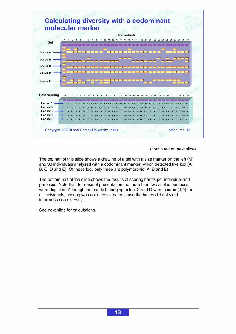
(continued on next slide)

The top half of this slide shows a drawing of a gel with a size marker on the left (M) and 30 individuals analysed with a codominant marker, which detected five loci (A, B, C, D and E). Of these loci, only three are polymorphic (A, B and E).

The bottom half of the slide shows the results of scoring bands per individual and per locus. Note that, for ease of presentation, no more than two alleles per locus were depicted. Although the bands belonging to loci C and D were scored (1,0) for all individuals, scoring was not necessary, because the bands did not yield information on diversity.

See next slide for calculations.

14


0.22

Hi

0.46

0.41

0.23

hj =

(1 - p2 - q2)

0.37

q

0.72

q

0.87

q

0.63

p

0.28

p

0.13

p

Allele

freq.

1

30

1

Total

1

30

1

Total

1

30

1

Total

E2 E2E1 E2E1 E1Genotypes

Eq22pqp2Gen. freq. (exp.)

7815Individuals (no.)

P22 = 0.23P12 = 0.27P11 = 0.50Gen. freq. (obs.)

B2 B2B1 B2B1 B1Genotypes

Bq22pqp2Gen. freq. (exp.)


P22 = 0.67P12 = 0.10P11 = 0.23Gen. freq. (obs.)

P22 = 0.80P12 = 0.13P11 = 0.07Gen. freq. (obs.)

Data analysisLocus

2

p2

A1 A1


q22pqGen. freq. (exp.)

A2 A2A1 A2Genotypes

A

Calculating diversity with a codominant molecular marker (continued)

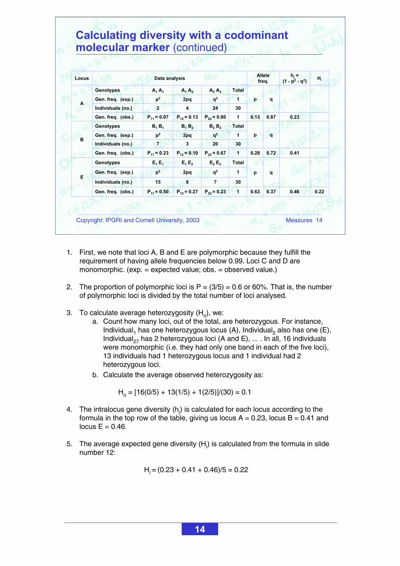
1. First, we note that loci A, B and E are polymorphic because they fulfill the requirement of having allele frequencies below 0.99. Loci C and D are monomorphic. (exp. = expected value; obs. = observed value.)

2. The proportion of polymorphic loci is P = (3/5) = 0.6 or 60%. That is, the number of polymorphic loci is divided by the total number of loci analysed.

3. To calculate average heterozygosity (Ho), we: a. Count how many loci, out of the total, are heterozygous. For instance,

Individual1 has one heterozygous locus (A), Individual2 also has one (E), Individual27 has 2 heterozygous loci (A and E), ... . In all, 16 individualswere monomorphic (i.e. they had only one band in each of the five loci), 13 individuals had 1 heterozygous locus and 1 individual had 2 heterozygous loci.

b. Calculate the average observed heterozygosity as:

Ho = [16(0/5) + 13(1/5) + 1(2/5)]/(30) = 0.1

4. The intralocus gene diversity (hj) is calculated for each locus according to the formula in the top row of the table, giving us locus A = 0.23, locus B = 0.41 and locus E = 0.46.

5. The average expected gene diversity (Hi) is calculated from the formula in slide number 12:

Hi = (0.23 + 0.41 + 0.46)/5 = 0.22

15


Locus A

Locus B

Locus E

Individuals

Locus C

Locus D

M 1 2 3 4 5 6 7 8 9 10 11 12 13 14 15 16 17 18 19 21 22 23 24 25 26 27 28 2920 30

Data scoring

1 0 1 0 0 0 0 0 0 1 0 0 0 0 0 1 0 0 0 0 0 0 0 1 0 0 1 0 0 0

M 1 2 3 4 5 6 7 8 9 10 11 12 13 14 15 16 17 18 19 21 22 23 24 25 26 27 28 2920 30

0 0 0 0 0 1 0 0 0 0 0 0 0 1 1 1 0 0 0 0 0 0 1 0 1 0 1 1 1 1

1 1 1 1 1 1 1 1 1 1 1 1 1 1 1 1 1 1 1 1 1 1 1 1 1 1 1 1 1 1

0 1 0 1 0 1 1 1 1 1 1 1 1 1 1 1 1 1 1 0 0 1 1 1 1 1 1 1 0 0

1 1 1 1 1 1 1 1 1 1 1 1 1 1 1 1 1 1 1 1 1 1 1 1 1 1 1 1 1 1

Locus A

Locus B

Locus E

Locus C

Locus D

Calculating diversity with a dominant molecular marker


The top half of this slide shows a drawing of a gel with a size marker on the left (M) and 30 individuals analysed with a dominant marker. Five loci are identified (A, B, C, D and E). Of the five loci detected, three are segregating (A, B and E), while the other two, C and D, are monomorphic.

The bottom half of the slide shows the results of scoring bands per individual and per locus. Because we are dealing with a dominant marker, bands are scored as 1 when present or 0 when absent. Scoring the bands for loci C and D can be either omitted or done as in the slide with ‘1’ for every individual.

The next slide shows the calculations.

16


0.198

Hi

0.50

0.30

0.19

hj =

(1 - p2 – q2)

0.48

q

0.82

q

0.89

q

0.52

p

0.18

p

0.11

p

Allele

freq.

1

30

1

Total

1

30

1

Total

1

30

1

Total

eeEeEEGenotypes

E

q22pqp2Gen. freq. (exp.)


P2 = 0.23P1 = 0.77Gen. freq. (obs.)

bbBbBBGenotypes

B

q22pqp2Gen. freq. (exp.)


P2 = 0.67P1 = 0.33Gen. freq. (obs.)

P2 = 0.80P1 = 0.20Gen. freq. (obs.)

Data analysisLocus

6

p2

Aa

24Individuals (no.)

q22pqGen. freq. (exp.)

aaAaGenotypes

A

Calculating diversity with a dominant molecular marker (continued)

1. First, we look at the polymorphism shown by all loci. Loci A, B and E fulfill the requirement of having allele frequencies below 0.99 and as such can be said to be polymorphic. Loci C and D are monomorphic. (exp. = expected value; obs. = observed value.)

2. The proportion of polymorphic loci (P) is P = (3/5) = 0.6 or 60%. The average heterozygosity (He) cannot be estimated because dominant markers do not allow discrimination between heterozygous and homozygous individuals.

3. Despite the above (2), the intralocus gene diversity (hj) may be calculated for each locus using the formula that appears in the top row of the table, column 4, as follows: locus A = 0.19; locus B = 0.30; and locus E = 0.50.

4. The average gene diversity (Hi) is calculated from the formula in slide number 12:

Hi = (0.19 + 0.30 + 0.50)/5 = 0.198

17


Interpopulation differentiation for one locus (gST)

Interpopulation differentiation for several loci (GST)

Population’s contribution to total genetic diversity

F statistics (Wright)

Analysis of molecular variance (AMOVA)

Quantifying genetic diversity: measuringinterpopulation genetic diversity

‘Differentiation’ refers to polymorphic differences between populations at different levels of structure (populations and individuals).

18


gST = 1 – (hS/hT)

hS = population diversity

hT = total diversity

Interpopulation differentiation for one locus (gST)

Where,hS = (ñ/(ñ - 1)[1 – (1/s) xij

2 – (ho/2ñ)]hT = 1 - [(1/s) xij]

2 + (hS/ñs) – (ho/2ñs)ñ = harmonic average of population sizes s = number of populationsho = average observed heterozygosityxij = estimated frequency of the ith allele in the jth population

• The formula in the slide provides a measure of differentiation in terms of alleles per locus in two or more populations

• It ranges from 0 to 1. A negative value may be obtained if an error was made for sampling or an inappropriate marker system was used.

• Because of the complexity of its components, its calculation requires specialized computer software.

• It can be used with codominant markers and restrictedly with dominant markers. This is because it is a measure of heterozygosity. To have a fair estimate of the real value, several generations are needed.

19


gST = 1 – (hs/hT) = 1 – (0.4196/0.8065) = 0.4797

hT = 1 – 0.1967 + [0.4196/(33.33 x 3)] – [0.20/(2 x 33.33 x 3)] = 0.8065

[1/3 xij]2 = (1/3(0.35))2 + (1/3(0.65))2 + (1/3(0.20))2 + … + (1/3(0.35))2 = 0.1967

hs = (33.33/33.33 – 1)[1 – 1/3(1.77) – (0.20/2(33.33))] = 0.4196

ñ = 33.331/ñ = 1/n1 + 1/n2 + 1/n3 = 1/100 + 1/100 + 1/100 = 0.03

(p2 + q2) = 1.77s = 3ho = 1/3(0.3 + 0.2 + 0.1) = 0.20

0.5450.350.65301060Pop. 3

0.6800.800.20702010Pop. 2

0.5450.650.35503020Pop. 1

p2 + q2qpA2 A2A1 A2A1 A1Genotypes

Calculating the gST

In this example, we have the number of individuals for each genotype for one locus (A) in three different populations. Using this number, we want to know the degree of differentiation in the three populations. In the table, the calculations are followed for all the necessary elements in the formula shown on the previous slide.

The result (gST = 0.4797) shows significant differentiation between populations in allele frequencies. We can therefore say that a high percentage of genetic diversity is distributed among populations.

20


HS HSDST

Pop1

Pop2

Pop3

HS

DST DSTHT

Interpopulation differentiation for several loci (GST)

GST is the coefficient of gene differentiation

GST = DST/HT

Where,HT = total genic diversity = HS + DST

HS = intrapopulation genic diversityDST = interpopulation diversity(HT/HT) = (HS/HT) + (DST/HT) = 1

• GST measures the proportion of gene diversity that is distributed among populations.

• A larger number of loci must be sampled.

• Equations are complex and should be calculated with specific computer software.

For example, assuming that:

HT = 0.263 HS = 0.202DST = 0.263 – 0.202 = 0.061

Then, GST = (DST/HT) 100 = (0.061/0.263) 100 = 23.19%. This means that, in this species, a 23% differentiation among populations exist.

21


The contribution is calculated by removing a population so that its contribution to the total gene diversity may be evaluated

CT(K) = (HT – HT/K)/HT

CS(K) = (HS – HS/K)/HT

CST(K) = (DST – DST/K)/HT

Population’s contribution to total gene diversity

Where,CT(K) = contribution of K to total diversityCS(K) = contribution of K to intrapopulation diversityCST(K) = contribution of K to interpopulation diversityHT = total gene diversityHS = intrapopulation genic diversityDST = interpopulation diversityHT/K = total gene diversity after removing population KHS/K = intrapopulation gene diversity after removing population K DST/K = interpopulation gene diversity after removing population K

• The measure allows quantifying the variation of total gene diversity when a population is introduced to or removed from a site (e.g. when introducing a new variety into a farmer’s field in an in situ conservation programme).

• It also serves to measure the impact of losing a population from a given site in terms of gene diversity.

• It can be used only with codominant markers.

22


The equation for the genetic structure of populations is:

(1 - FIT) = (1 – FIS)(1 – FST)

FIT = 1 – (HI/HT)

FIS = 1 – (HI/HS)

FST = 1 – (HS/HT)

F statistics (Wright)

Where,HT = total gene diversity or expected heterozygosity in the total population as estimated from the pooled allele frequenciesHI = intrapopulation gene diversity or average observed heterozygosity in a group of populations HS = average expected heterozygosity estimated from each subpopulation

The F statistics allow analysis of structures of subdivided populations. It may also be used to measure the genetic distance among subpopulations, a concept that is based on the idea that those subpopulations that are not intermating will have different allele frequencies to those of the total population.

Genetic distance also provides a way of measuring the probability of encounter between equal alleles (endogamy). The statistical indexes involved measure:

FIS = the deficiency or excess of average heterozygotes in each populationFST = the degree of gene differentiation among populations in terms of allele frequencies FIT = the deficiency or excess of average heterozygotes in a group of populations

23


The range of the FST is:

10

(fixation for alternate

alleles in different

subpopulations)

(no genetic divergence)

When FST is: then the genetic differentiation is:

0 to 0.05 small 0.05 to 0.15 moderate0.15 to 0.25 large>0.25 very large

Interpreting FST values

24


(0.495 + 0.420)/2 = 0.4575

Genotype frequency

HS

(0.45 + 0.30)/2 = 0.375qo(0.3 + 0.2)/2 = 0.25HI

(0.55 + 0.70)/2 = 0.625po2(0.625)(0.375) = 0.4688HT

0.52380.42000.300.700.200.200.602

0.39390.49500.450.550.300.300.401

F2piqiqipiA2 A2A1 A2A1 A1

Pop.

FIT = 1 – (0.25/0.4688) = 0.4667

FIS = 1 – (0.25/0.4575) = 0.4536

FST = 1 – (0.4575/0.4688) = 0.0241

Calculating F statistics


This slide shows an example of two populations and the analysis of one locus (A). The allele frequencies are calculated (p and q), as are their averages. The variables HT, HI and HS are also estimated and used to calculate the F statistics. The analysis shows low differentiation in allele frequencies among the two populations (FST). We could conclude that almost all the heterozygote deficit was due to nonrandom mating within the populations (FIS = 0.4536).

F = fixation index (first column on right of table) is the probability that two alleles carried by one individual will be the same. It should be calculated only with codominant markers. If done with dominant markers, a biased estimator may result.

25


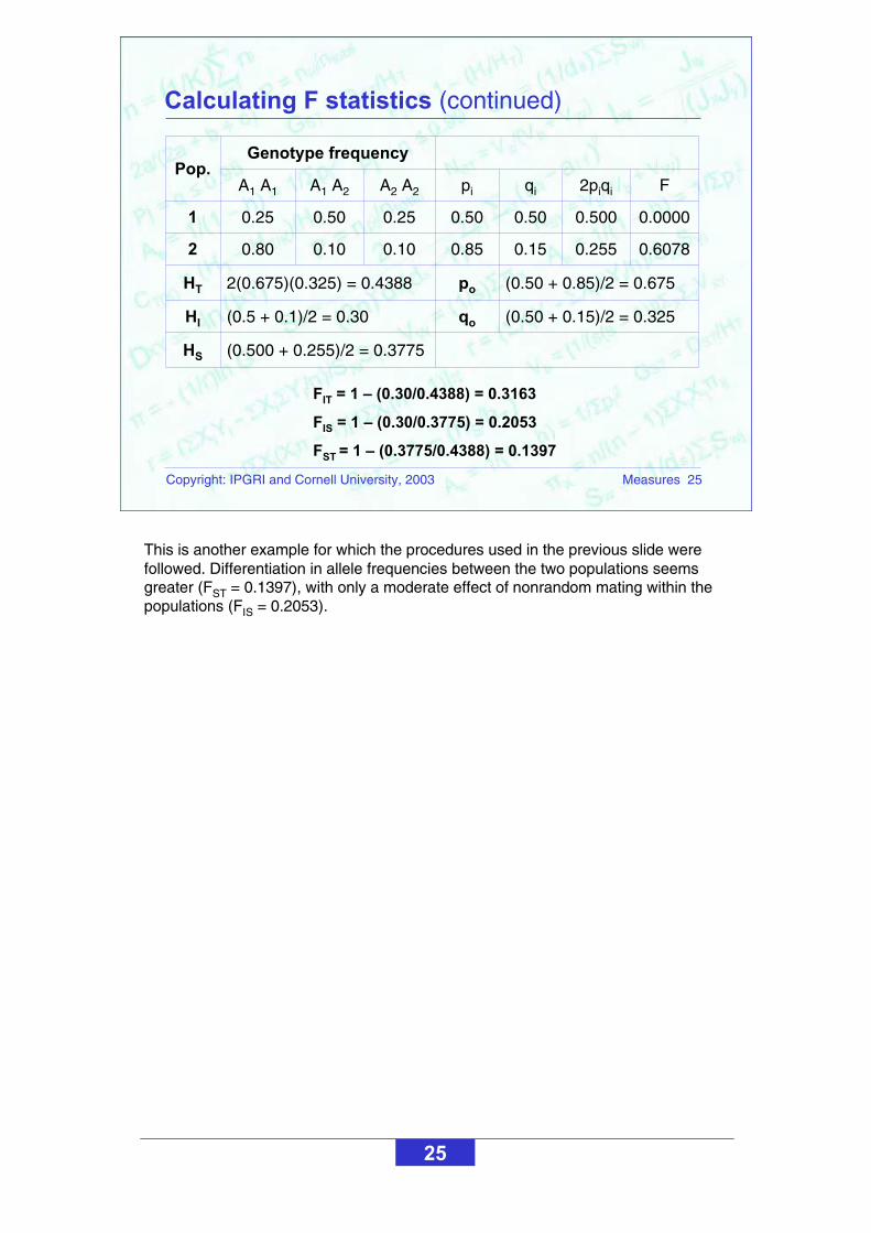
qo

Genotype frequency

(0.500 + 0.255)/2 = 0.3775HS

(0.50 + 0.15)/2 = 0.325(0.5 + 0.1)/2 = 0.30HI

(0.50 + 0.85)/2 = 0.675po2(0.675)(0.325) = 0.4388HT

0.60780.2550.150.850.100.100.802

0.00000.5000.500.500.250.500.251

F2piqiqipiA2 A2A1 A2A1 A1

Pop.

FIT = 1 – (0.30/0.4388) = 0.3163

FIS = 1 – (0.30/0.3775) = 0.2053

FST = 1 – (0.3775/0.4388) = 0.1397

Calculating F statistics (continued)

This is another example for which the procedures used in the previous slide were followed. Differentiation in allele frequencies between the two populations seems greater (FST = 0.1397), with only a moderate effect of nonrandom mating within the populations (FIS = 0.2053).

26


AMOVA is a method for studying molecular variation within a species

It is based on a hierarchical or nested model

It differs from an analysis of variance (ANOVA)in that:

• It may contain different evolutionary assumptions without modifying the basic structure of the analysis

• The driving hypothesis uses permutational methods that do not require the assumption of a normal distribution

Analysis of molecular variance (AMOVA)

The different hierarchical levels of gene diversity studied through AMOVA may include:

1. Continents, which may contain lesser hierarchical levels

2. Geographical regions within a continent

3. Areas within a region in a continent

4. Populations within an area of a region in a continent

5. Individuals within a population in an area of a region in a continent

The mathematical description of the model for situations 3 and 4 can be found in Appendices 2 and 3, respectively.

The next two slides illustrate how to analyse situation 4.

27


01101115

01011114

10111113

01110012

11100111

10011110

0111019

0011008

1111117

0010006

1010005

1101014

1011003

1110112

1110001

A2

A1

A2

A1

A2

A1

Pop. 3Pop. 2Pop. 1Ind.

AbsentA1 = 0

PresentA1 = 1

2916X...2

54182115Xijk2

88283327Xi...k2

990324441225X...k2

54182115X...k

0.22222222MSw10SSw

0.26190476MSb11SSb

0.3MSa0.6SSa

An example of AMOVA


In this table, we show data obtained with 15 individuals from each of three populations in an analysis with a codominant marker. By means of an analysis of variance, these data will allow us to calculate the F statistics.

The first step is to convert the bands detected in the gels to binary variables with a value of either 0 or 1. Then, the sums of presences (1) are calculated so we may proceed with the sum of squares. Calculations are first done for one population and continued for the others until we have (X...k). We have i = 15 individuals (effect b), j = 2 alleles (effect w), k = 3 populations (effect a).

Where,X...k is the result of summing up all the band presences (1) in the individuals per populationX...k

2 is the result of squaring the number obtained aboveXi...k

2 is the result of adding up the squares of the sum of allele presences in each individual (e.g. Indiv.1 in Pop.1 will be (0 + 0)2 + Indiv.2in Pop.1 (1 + 1)2 + Indiv. ...)

Xijk2 is the sum of each value squared

SS is the sum of squares for effects a, b and wAn example of calculating SS: SSa = X...k

2/ij – X...2/ijk = [990/(15 x 2)] - [2916/(15 x 2 x 3)] = 0.6MS are the mean squares for effects a, b and wAn example of calculating MS: SSa/dfa = 0.6/2 = 0.3, where dfA refers to the degrees of freedom for effect a (populations).

28


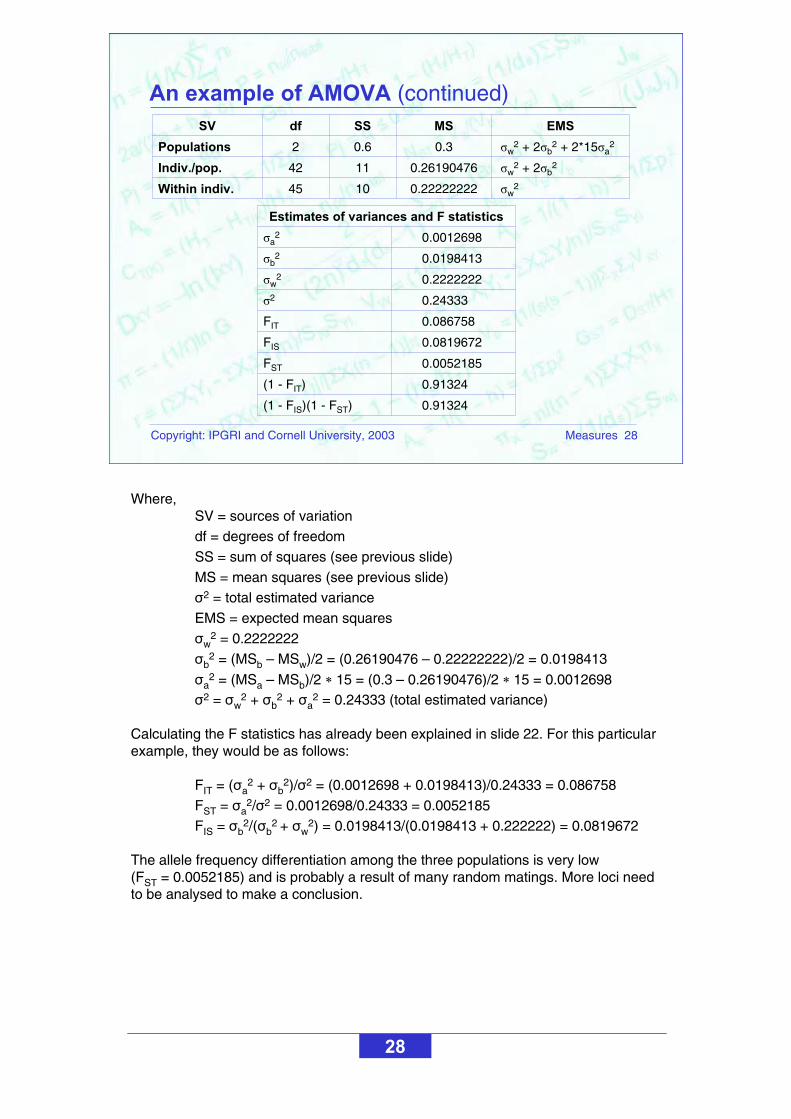
w20.222222221045Within indiv.

w2 + 2 b

20.261904761142Indiv./pop.

w2 + 2 b

2 + 2*15 a20.30.62Populations

EMSMSSSdfSV

0.91324(1 - FIS)(1 - FST)

0.91324(1 - FIT)

0.0052185FST

0.0819672FIS

0.086758FIT

0.243332

0.2222222w2

0.0198413b2

0.0012698a2

Estimates of variances and F statistics

An example of AMOVA (continued)

Where,SV = sources of variationdf = degrees of freedomSS = sum of squares (see previous slide)MS = mean squares (see previous slide)

2 = total estimated variance EMS = expected mean squares

w2 = 0.2222222

b2 = (MSb – MSw)/2 = (0.26190476 – 0.22222222)/2 = 0.0198413

a2 = (MSa – MSb)/2 15 = (0.3 – 0.26190476)/2 15 = 0.0012698

2 = w2 + b

2 + a2 = 0.24333 (total estimated variance)

Calculating the F statistics has already been explained in slide 22. For this particular example, they would be as follows:

FIT = ( a2 + b

2)/ 2 = (0.0012698 + 0.0198413)/0.24333 = 0.086758FST = a

2/ 2 = 0.0012698/0.24333 = 0.0052185FIS = b

2/( b2 + w

2) = 0.0198413/(0.0198413 + 0.222222) = 0.0819672

The allele frequency differentiation among the three populations is very low (FST = 0.0052185) and is probably a result of many random matings. More loci need to be analysed to make a conclusion.

29


Using sequence data• Intrapopulation nucleotide diversity• Interpopulation nucleotide diversity

Using restriction data• Variations in banding patterns• Intrapopulation nucleotide diversity• Interpopulation nucleotide diversity

Quantifying genetic relationships: diversityand differentiation at the nucleotide level

For these calculations, the assumption is made that each nucleotide is a locus.

30


It measures the nucleotide diversity among several sequences in a given region of the genome within a population ( X)

X = n/(n – 1) XiXj ij

Using sequence data: intrapopulationnucleotide diversity

Where,n = number of sequences under analysis in the individuals of thepopulationXi = estimated frequency of the ith sequence in the population Xj = estimated frequency of the jth sequence in the population

ij = proportion of different nucleotides between sequences i and j

• The measure informs about the degree of nucleotide diversity among several sequences in a given region of the genome. It is equivalent to the measure of allelic diversity within a locus.

• It ranges from 0 to 1 (0 X 1).

• The factors limiting the use of this analytical tool are:

Partial genomic sequences must be availableThe equation can only be applied to haploid data

This parameter informs about nucleotide sequences, and the model assumes haplotypes (haploid genotypes). Even if the study is based on diploid individuals, sequencing of each copy of the genome is needed.

31


10

2

1

2

5

n

2/10 = 0.2TCC G CGAT T ATTC T CAGGGTGC G GATG A ATSeq4

1/10 = 0.1TCC A CGAT C ATTC C CAGGGTGC A GATG G ATSeq3

2/10 = 0.2TCC A CGAT T ATTC G CAGGGTGC C GATG A ATSeq2

5/10 = 0.5TCC T CGAT T ATTC C CAGGGTGC C GATG A ATSeq1

Freq. XiSequence

1,2 = 2/30, 1,3 = 4/30, 1,4 = 3/30, 2,3 = 4/30, 2,4 = 3/30, 3,4 = 5/30

X = 10/(10 – 1) XiXj ij

= (10/9)[0.5 0.2 (2/30) + 0.5 0.1 (4/30) + ... + 1 0.2 (5/30)]

= 0.037

Calculating intrapopulation nucleotide diversity

This example has 10 individuals in a population X. For each individual, we analyse one sequence of 30 nucleotides, and find that individual sequences differ at 5 nucleotide positions (blue). In total, 4 alternative sequences for those 30 nucleotides are present in the population. In the first column, we note the number of individuals (n) that have the particular sequence alternatives.

Then, we calculate the number of nucleotide differences in each sequence pair within the population. For example, 1,2 = 2/30 means that between sequence 1 and 2 there are two nucleotide differences (T vs. A in position 4, and C vs. G in position 14).

Next, we calculate X for the entire population. The number obtained is 0.037, or 3.7% nucleotide diversity, based on the sequence analysed in the sample of 10 individuals.

32


VXY measures population divergence based on the degree of sequence variation (1 sequence, 2 populations)

VXY = dXY – ( X + Y)/2

VW measures average diversity in a population based on several sequences

VW = (1/s) X

Vb measures the total differentiation in several populations

Vb = [1/(s(s – 1))] X YVXY

NST is the relative differentiation

NST = Vb/(Vb + VW)

Using sequence data: interpopulationnucleotide diversity

Where,VXY = divergence among populations X and Y

X = nucleotide diversity in population XdXY = the probability that two random nucleotides in populations X and Y be different s = number of populations

• The measure informs about the level of differentiation among nucleotide sequences in populations.

• It requires sequence data in a sample of individuals for each population.

• It needs specific computer software that includes sequence alignment features.

Some of these are CLUSTAL W, MALIGN and PAUP*.

33


Relative differentiation

NST = Vb/(Vb + VW) = 0.03825/(0.03825 + 0.0635) = 0.3759

Average diversity in each population

VW = (1/s) X = ½(0.037 + 0.09) = 0.0635

Total differentiation

Vb = [1/(s(s – 1))] X YVXY = [1/(2(2 – 1))]0.0765 = 0.03825

Nucleotide divergence between X and Y

VXY = dXY – ( X Y)/2 = 0.14 – (0.037 + 0.09)/2 = 0.0765

Calculating interpopulation nucleotide diversity

Let’s say that we have another population Y, in which the nucleotide diversity for the same sequence analysed in slide 31 is Y = 0.09.

We also know that the probability that two nucleotides as taken at random are different in X and Y is 0.14 (dXY).

In this slide, we find the divergence between populations X and Y (VXY), the total differentiation (Vb), the average diversity in each population (Vw) and the relative differentiation (NST)..

34


…GACTGAATTCCACGGCACTGACGAATTCGA…AGTGAATTCTTACTTAAGCTAGCCTGAATTCGATAC…

…CTGACTTAAGGTGCCGTGACTGCTTAAGCT…TCACTTAAGAATGAATTCGATCGGACTTAAGCTATG…

…GACTGATTTCCACGGCACTGACGAATTCGA…AGTGAATTCTTACTTAAGCTAGCCTGAATTCGATAC…

…CTGACTAAAGGTGCCGTGACTGCTTAAGCT…TCACTTAAGAATGAATTCGATCGGACTTAAGCTATG…

DNA

Indiv. 1

DNA

Indiv. 2

Restriction site EcoRI

No recognition

site for EcoRI

Fragment 1 Fragment 2

Fragment 2

M I1 I2

Gel

Fragment 2

Fragment 1

Using restriction data: variations in banding patterns

The lack of fragment 1 in Individual2 indicates that it carries a different DNA sequence at least in that restriction site. A small difference of just two nucleotides, in the drawing above, is sufficient to make the recognition site for the enzyme to disappear.

35


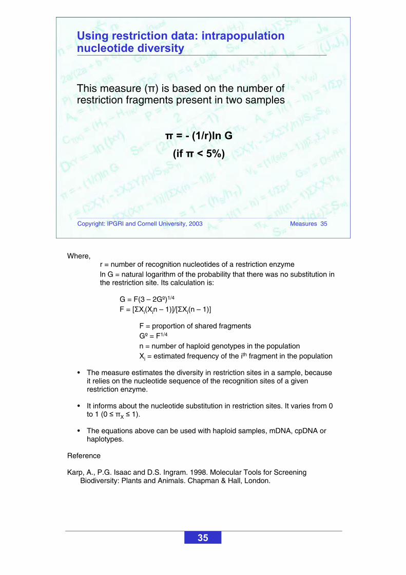
This measure ( ) is based on the number of restriction fragments present in two samples

= - (1/r)ln G

(if < 5%)

Using restriction data: intrapopulationnucleotide diversity

Where,r = number of recognition nucleotides of a restriction enzymeln G = natural logarithm of the probability that there was no substitution in the restriction site. Its calculation is:

G = F(3 – 2Gº)1/4

F = [ Xi(Xin – 1)]/[ Xi(n – 1)]

F = proportion of shared fragmentsGº = F1/4

n = number of haploid genotypes in the population Xi = estimated frequency of the ith fragment in the population

• The measure estimates the diversity in restriction sites in a sample, because it relies on the nucleotide sequence of the recognition sites of a given restriction enzyme.

• It informs about the nucleotide substitution in restriction sites. It varies from 0 to 1 (0 X 1).

• The equations above can be used with haploid samples, mDNA, cpDNA or haplotypes.

Reference

Karp, A., P.G. Isaac and D.S. Ingram. 1998. Molecular Tools for Screening Biodiversity: Plants and Animals. Chapman & Hall, London.

36


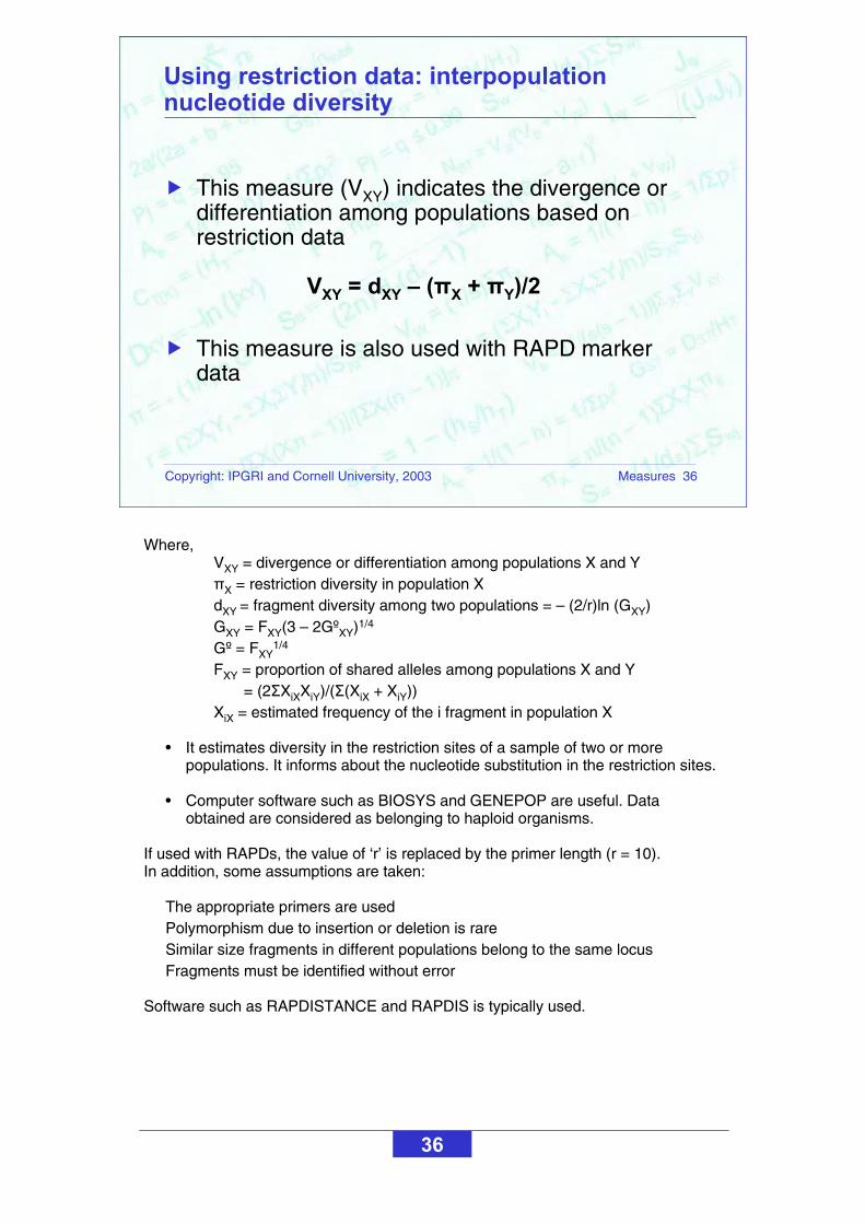
This measure (VXY) indicates the divergence or differentiation among populations based on restriction data

VXY = dXY – ( X + Y)/2

This measure is also used with RAPD marker data

Using restriction data: interpopulationnucleotide diversity

Where,VXY = divergence or differentiation among populations X and Y

X = restriction diversity in population XdXY = fragment diversity among two populations = – (2/r)ln (GXY) GXY = FXY(3 – 2GºXY)1/4

Gº = FXY1/4

FXY = proportion of shared alleles among populations X and Y = (2 XiXXiY)/( (XiX + XiY))

XiX = estimated frequency of the i fragment in population X

• It estimates diversity in the restriction sites of a sample of two or more populations. It informs about the nucleotide substitution in the restriction sites.

• Computer software such as BIOSYS and GENEPOP are useful. Data obtained are considered as belonging to haploid organisms.

If used with RAPDs, the value of ‘r’ is replaced by the primer length (r = 10). In addition, some assumptions are taken:

The appropriate primers are usedPolymorphism due to insertion or deletion is rareSimilar size fragments in different populations belong to the same locusFragments must be identified without error

Software such as RAPDISTANCE and RAPDIS is typically used.

37


Calculating interpopulation nucleotide diversity

Population

X X = -(1/6) ln (0.039358) = 0.539176

G = 0.0325[3 – 2(0.424591)]1/4 = 0.039358G° = (0.0325)1/4 = 0.424591

F = [0.30(0.30 3 – 1) + 0.25(0.25 3 – 1) + 0.45(0.45 3 – 1)] = 0.0325

0.30(3 – 1) + 0.25(3 – 1) + 0.45(3 – 1)

9/20 = 0.45A3

5/20 = 0.25A2

6/20 = 0.30A1

Freq. Xi2019181716151413121110987654321Seq.

Population

Y Y = -(1/6) ln (0.272587) = 0.216633

G = 0.2425[ 3 – 2(0.701743)]1/4 = 0.272587G° = (0.2425)1/4 = 0.701743

F = [0.25(0.25 3 – 1) + 0.65(0.65 3 – 1) + 0.10(0.10 3 – 1)] = 0.2425

0.25(3 – 1) + 0.65(3 – 1) + 0.10(3 – 1)

2/20 = 0.10A3

13/20 = 0.65A2

5/20 = 0.25A1

Freq. Xi2019181716151413121110987654321Seq.

In each population, we detected three DNA fragments as a result of a restriction digest: A1, A2 and A3.

Nucleotide diversity in the regions analysed is larger in population X ( X = 0.5392)than in population Y ( Y = 0.2166); thus, X has more gene diversity than Y.

Between populations X and Y, the nucleotide differentiation based on restriction sites is 0.230766.

0.6130521/4

0.14125XYG

0.141250.100.450.650.250.250.300.10*0.450.65*0.250.25*0.302

F

163012.04/1613052.02314125.0GXY

604643.0163012.0ln6/2dXY

226739.0216633.0539176.02

1604643.0VXY

377905.0216633.0539176.02

1VW

11337.0226739.02

1Vb

0.2307660.3779050.11337

0.11337NST

38


The genetic distance between two samples is described as the proportion of genetic elements (alleles, genes, gametes, genotypes) that the two samples do not share

D = 1 when, and only when, the two samples have no genetic elements in common

Quantifying genetic relationships: geneticdistance

Depending on the similarities of individuals, three representation types of distance (D) are possible:

• D = 1 – S, known as linear distance, because it assumes that the relationship with similarity is linear.

• D = (1 – S), known as quadratic distance because it assumes that the relationship with similarity follows a quadratic function, so that, to make it linear, the square root must be calculated.

• D = (1 – S2), known as circular distance.

Linear

0

0.2

0.4

0.6

0.8

1

0 0.2 0.4 0.6 0.8 1

Similarity

Dis

tan

ce

Quadratic

0

0.2

0.4

0.6

0.8

1

0 0.2 0.4 0.6 0.8 1

Similarity

Dis

tan

ce

R

0

0.2

0.4

0.6

0.8

1

0 0.2 0.4 0.6 0.8 1

Similarity

Dis

tan

ce

Linear Quadratic Circular

39


Calculation of distance, or dissimilarity, follows one of two possible models:

Equilibrium model

Distance remains constant over time (equilibrium exists between

migration and genetic drift)

Distance changes with time through migration and

genetic drift

d

d

t

t + 1t + 1

d2

d1

t

Disequilibrium model

Distance models

For our purposes, we will use the disequilibrium model. Two alternatives exist:

• Geometric distanceDoes not take into account evolutionary processes Based only on allele frequencies Complex relationship exists between distance and divergence time

• Genetic distanceDoes not take into account evolutionary processes Distance increases from the time of separation from an ancestral population A genetic model of evolution is needed

When should we use geometric or genetic distance?

• Geometric distance is used for diversity studies in which comparisons are made according to morphological or marker data gathered from the operative taxonomic units (OTUs). OTUs may be individuals, accessions or populations. It can be used with dominant markers (RAPDs, AFLPs) or codominant markers. Because evolutionary aspects are not considered, the dendrograms obtained cannot be interpreted as phylogenetic trees giving information about evolution or divergence among groups.

• In contrast, the genetic distance of any given OTU can be incorporated into phylogeny studies. The model considers allelic frequencies in OTUs and its mathematical foundation is different. It can be used with both codominant and dominant markers, although, with the latter, information is lost because only two alleles can be scored. Genetic distance with dominant markers, however, requires the examination of two generations of the same population to measure the segregation of loci (Lynch and Milligan, 1994).

Reference

Lynch, M. and B.G. Milligan. 1994. Analysis of population genetic structure with RAPD markers. Mol. Ecol. 3:91-99.

40


Disequilibrium models: geometric distance

This measures the direct relationship between the similarity index (s) and distance (D = 1 – s)

Different situations are possible, for example:• Binary variables• Quantitative variables • Mixed types of variables• P number of variables


When analysing molecular data, we deal with binary variables (1,0). These will be discussed in the following slides.

In Appendix 4, you will find additional information for those cases where you also must deal with quantitative variables, mixed types of variables and a varied number of variables. In Appendix 5, an example of calculating geometric distances withquantitative variables has also been added.

41


With binary variables: • Multivariate analysis is used and similarity or

differentiation matrices are formed between the possible pairs of individuals or operative taxonomic units (OTUs)

• Two similar individuals simultaneously have the minimum value of distance and the maximum value of similarity

• Distance and similarity are inversely related • Similarity is estimated by the number of coincidence

Geometric distance (continued)

When using molecular marker data and transforming them to binary data, the following should be considered:

• A species’s ploidy number may mask the presence of allelic series in a locus. If this happens, genetic diversity will be underestimated when using dominant markers (presence/absence).

• If a marker is codominant, large samples are needed to permit detection of all possible genotypes, particularly if there are several alleles per locus.

• Segregation distortions are common in polyploid species.

• Most specialized computer software are designed to analyse diploid species. Therefore if used with polyploid species, biases may occur on estimating the various genetic diversity indices.

• The reproductive system of certain species has not been studied, so their inheritance type is not sufficiently known.

• The largest coverage (coding and non-coding regions) possible of the genome of the species under study should be sampled and analysed so that estimates of genetic diversity are reliable.

42


Locus A

diploid

(2X)

Locus A

tetraploid

(4X)

Individuals

M 1 2 3 4 5 6 7 8 9 1810 11 12 1716151413

Calculating allele frequencies for diploids and tetraploids: dominant marker

M 1 2 3 4 5 6 7 8 9 1810 11 12 1716151413

1 1 0 1 1 1 1 0 1 1 1 0 1 1 1 0 1 1

1 1 0 1 1 1 1 0 1 1 1 0 1 1 1 0 1 1

Binary

matrix

Allele freq.GenotypesLocu

s

0.69

q

0.47

q

0.31

p

0.53

p

TotalaaaaAAAA, AAAa, AAaa,

AaaaTetraploid

A

(4X)1q4p4 + 4p3q + 6p2q2 +

4pq3Gen. freq. (e.)

18414Indiv. number

1P2 = 0.22P1 = 0.78Gen. freq. (o.)

1P2 = 0.22P1 = 0.78Gen. freq. (o.)

14

p2 + 2pq

AA, Aa

184Indiv. number

1q2Gen. freq. (e.)

TotalaaDiploid

A

(2X)

Allele frequencies should be different in both cases; however, the information loss in the tetraploid individual is significant. Why? This is because, to estimate the frequency of the recessive allele a, heterozygotes AAAa, AAaa, Aaaa are not taken into account. This effect is larger when the ploidy number of the species under study is unknown. (e. = expected value; o. = observed value.)

This example of 18 individuals from each of a diploid and a tetraploid species was analysed with a dominant marker. We are assuming that the banding patterns obtained are alike. Bands are converted to a binary table in both cases. The calculations of the frequencies are given in the table below. We can see that, in thetetraploid, genotype 1, for example, can be either AAAA, AAAa, AAaa or Aaaa; however the band will only be scored as present (1) the same as it will in the diploid (AA or Aa).

43


Locus A

diploid

(2X)

Locus A

tetraploid

(4X)

Diploid

binary

matrix

I N D I V I D U O S

(1,0,0) (1,0,1) (0,0,1) (1,0,1) (0,1,1) (1,0,0) (1,0,1) (0,0,1) (0,0,1) (0,1,0) (1,1,0) (0,0,1) (0,0,1) (0,0,1) (0,0,1) (0,1,1) (1,0,1) (0,0,1)

M 1 2 3 4 5 6 7 8 9 1810 11 12 1716151413

Calculating allele frequencies for diploids and tetraploids: codominant marker

Individuals

A1

A1

A1

A1

A1

A1

A2

A3

A1

A2

A2

A3

A1

A2

A3

A3

A3

A3

A3

A3

M 1 2 3 4 5 6 7 8 9 1810 11 12 1716151413

A1

A1

A1

A2

A1

A3

A2

A2

A2

A3

A3

A3

In this example, we have 18 individuals from each of a diploid and tetraploid species and analysed with a codominant marker. One locus is detected (A) with three alleles in both situations (A1, A2 and A3).

Calculating the allele frequencies in the diploid individual is not difficult (binary matrix, bottom of slide). For the tetraploid individual, however, conversion to binary data is hampered by the fact that individuals with alleles A1 A1 A2 A3 cannot be distinguished from those with other combinations such as A1 A2 A2 A3 or A1 A2 A3A3. This situation can only be solved by inference based on estimating the DNA fragment copy number in the gel.

0.25

p

0.15

q

1

18

1

Tota

l

P13 =

0.22

4

2pr

A1

A3

P22 =

0.06

1

q2

A2

A2

P23 =

0.11

2

2qr

A2

A3

0.60

r

P33 =

0.44

P12 =

0.06

P11 =

0.11

Gen. freq.

(o.)

2

p2

A1 A1

81Indivs. (no.)

r22pqGen. freq.

(e.)

A3

A3

A1

A2

Genotype

(e. = expected value; o. = observed value.)

44


1.250(a + d)/(b + c)Sokal and Sneath 3 (1963)S13

0.714(a + d)/[a + d + (b + c)/2]Sokal and Sneath 1 (1963)S12

0.385(a + d)/[a + d + 2(b + c)]Rogers and Tanimoto (1960)S11

0.556(a + d)/nSokal and Michener (1958)S10

0.750a/(b + c)Kulczynski 1 (1928)S9

0.273a/[a +2(b + c)]Sokal and Sneath 5 (1963)S8

0.429a/(a + b + c)Jaccard (1900, 1901, 1908)S7

0.625(a/2)([1/(a+b)] + [1/(a+c)])Kulczynski 2S6

0.612a/[(a + b)(a + c)]1/2Ochiai (1957)S5

0.600a/[a + (b + c)/2]Dice (1945); Nei and Li (1979)S4

0.500a/max[(a + b),(a + c)]Braun-BlanquetS3

0.750a/min[(a + b),(a + c)]SimpsonS2

0.333a/nRussel and Rao (1940)S1

Example of the coefficient value

if

a = 3, b = 1, c = 3, d = 2

ExpressionAuthor

Similarity coefficients for binary variables:

examples

Where, n = a + b + c + d

In the table above we see that:

Indices S1 to S9 give value only to the presence of informationIndices S10 to S13 give value to both presence and absence

Next, we will discuss three indices (in red on top table): Simple Matching (S10), Jaccard (S7) and Nei-Li (S4).

c + ddc0

a +

bba1

Indiv.i

b + d

0

a + c

1

Indiv.j

n

45


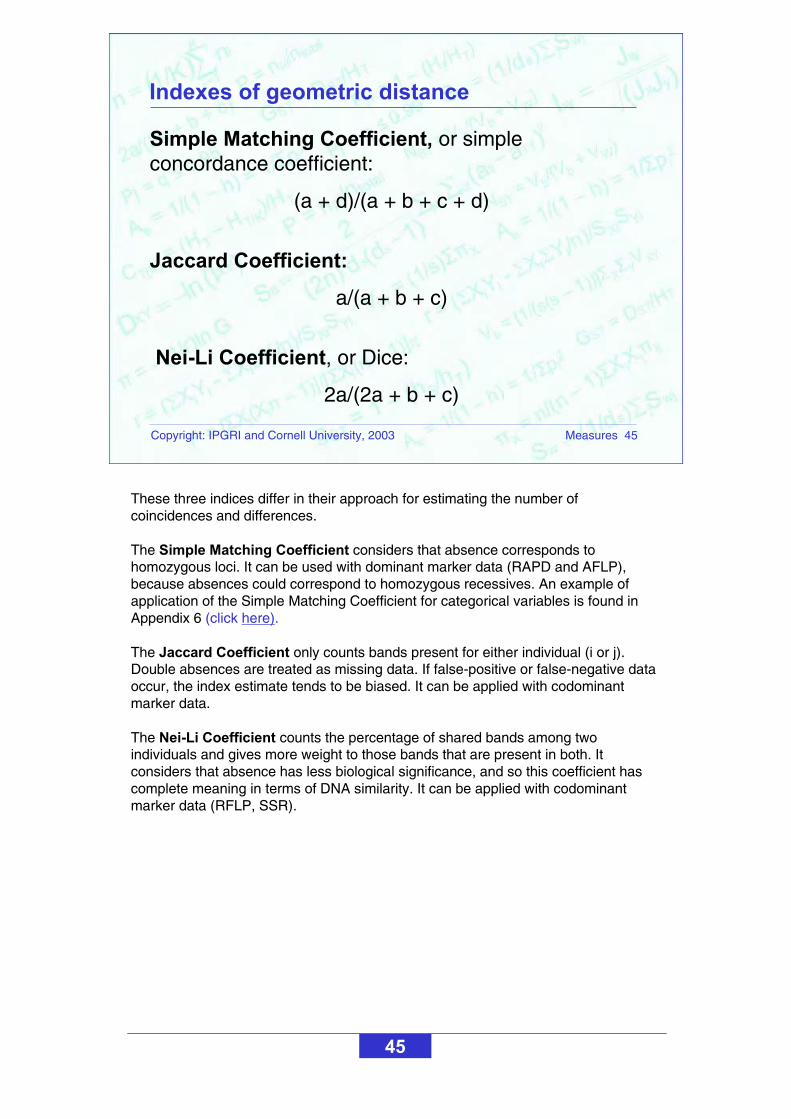
Simple Matching Coefficient, or simple concordance coefficient:

(a + d)/(a + b + c + d)

Jaccard Coefficient:

a/(a + b + c)

Nei-Li Coefficient, or Dice:

2a/(2a + b + c)

Indexes of geometric distance

These three indices differ in their approach for estimating the number of coincidences and differences.

The Simple Matching Coefficient considers that absence corresponds to homozygous loci. It can be used with dominant marker data (RAPD and AFLP), because absences could correspond to homozygous recessives. An example of application of the Simple Matching Coefficient for categorical variables is found in Appendix 6 (click here).

The Jaccard Coefficient only counts bands present for either individual (i or j). Double absences are treated as missing data. If false-positive or false-negative data occur, the index estimate tends to be biased. It can be applied with codominant marker data.

The Nei-Li Coefficient counts the percentage of shared bands among two individuals and gives more weight to those bands that are present in both. It considers that absence has less biological significance, and so this coefficient has complete meaning in terms of DNA similarity. It can be applied with codominant marker data (RFLP, SSR).

46


Measures the difference between two genes, proportional to the time of separation from a common ancestor

Several models are possible:• Mutation of infinite alleles

e.g. Nei’s genetic distance

• Stepwise mutation modele.g. Distance using microsatellites

• Mutation in the nucleotide sequence

Disequilibrium models: genetic distance

• Mutation of infinite alleles (i.e. isozymes)Each mutation event gives rise to a new allele. If 2 genes are the same, no mutation has occurred. If 2 genes are different, an unknown number of mutations occurred.The average number of mutations since time t when they diverged from an ancestor is = 2tµ, where µ is the rate of mutation and is multiplied by 2 because we are dealing with 2 independent genes.The probability that 2 genes are common by descent after time t is P= e-2tµ.

• Stepwise mutation model (i.e. SSRs)Mutation is a progressive change so fragments that migrate similar distances have had few mutations.In the case of SSRs, mutation is assumed to change the number ofrepeats, increasing or decreasing step by step. It can be shown that the square of the difference in the number of repeats between 2 microsatellites is proportional to the time of divergence from a common ancestor.

• Mutation in the nucleotide sequence It indicates that the simplest substitution is the mutation of a single base.The main limitation is the loss of information by not knowing the number of mutations that could have taken place at one site. To solve that problem, some methods assume the probability of transition (purine purine or pyrimidine pyrimidine) and transversion (purine pyrimidine or pyrimidine purine).

47


The standard Nei’s genetic distance is:

It is based on the concept of genetic identity (IXY):

)J(J

JI

yx

xyxy

)(IlnD XYXY

Calculating Nei’s genetic distance


Where,JX = average homozygosity in population XJY = average homozygosity in population YJXY = average interpopulation homozygosity

Such that,IXY = 1, if two populations have the same allele frequencies in all sampled lociIXY = 0, if two populations do not share the same allele frequencies in all sampled loci

• The value of DXY varies from 0 (where populations have identical allele frequencies) to infinity ( , where populations do not share any alleles).

• It assumes that the rate of substitution per locus is equal among all loci and populations.

• This distance estimates the codon differences per locus between two populations.

48


D2,3 = 0.0440D1,3 = 0.0107D1,2 = 0.0852Dii’Genetic distance

I2,3 = 0.9570I1,3 = 0.9894I1,2 = 0.9183Iii’Genetic identity

J2,3 = 0.8986J1,3 = 0.9346J1,2 = 0.8733Jii’Average interpop. homozygosity

0.93270.94530.9567JiAverage homozygosity

0.06730.05470.0433HiAverage heterozygosity

0.42000.000.0000hijkLocus heterozygosity

0.700.001.00D2

0.301.000.00D1D


0.000.090.13B3

0.000.100.01B2

1.000.810.86B1B


0.350.260.20A2

0.650.740.80A1A

Pop.3Pop.2Pop.1

Allele frequenciesAllelesLocus

Calculating Nei’s genetic distance (continued)

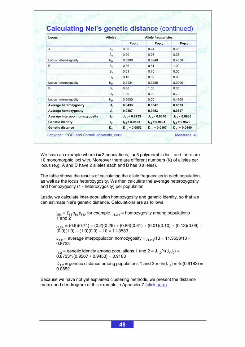
We have an example where i = 3 populations, j = 3 polymorphic loci, and there are 10 monomorphic loci with. Moreover there are different numbers (K) of alleles per locus (e.g. A and D have 2 alleles each and B has 3 alleles).

The table shows the results of calculating the allele frequencies in each population, as well as the locus heterozygosity. We then calculate the average heterozygosity and homozygosity (1 - heterozygosity) per population.

Lastly, we calculate inter-population homozygosity and genetic identity, so that we can estimate Nei’s genetic distance. Calculations are as follows:

jii’jk = ii’j pijk pi’jk, for example, j1,2jk = homozygosity among populations 1 and 2

j1,2jk = (0.8)(0.74) + (0.2)(0.26) + (0.86)(0.81) + (0.01)(0.10) + (0.13)(0.09) + (0.0)(1.0) + (1.0)(0.0) + 10 = 11.3533

J1,2 = average interpopulation homozygosity = j1,2jk/13 = 11.3533/13 = 0.8733

I1,2 = genetic identity among populations 1 and 2 = J1,2/ (J1J2) = 0.8733/ (0.9567 0.9453) = 0.9183

D1,2 = genetic distance among populations 1 and 2 = -ln(I1,2) = -ln(0.9183) = 0.0852

Because we have not yet explained clustering methods, we present the distance matrix and dendrogram of this example in Appendix 7 (click here).

49


i'i2

i'i'iiwi )a(a1)2n(2n

2S

j wjsw S)(1/dS

Calculating intrapopulation distance, using microsatellites

Intrapopulation distance is the average of the sum of squares of the differences in the number of repeats between alleles

The average intrapopulation distance may becalculated for all analysed loci (ds)

Where,aij = size of the allele of the ith copy (i = 1, 2, …, 2n) in the jth population (j = 1, 2, …, ds)n = number of individuals in the sample

Two considerations:

The calculation of distance between two alleles is a transformation of the number of repeats. One difficulty in using SSRs to estimate genetic distances is their high rate of mutation.

50


This is the interpopulation component for the average distance among all allele pairwise comparisons

j'j i'i2

j'i'ij

ss2

B )a(a1)(dd(2n)

2S

Calculating interpopulation distance, using microsatellites

The global distance is the weighted average among the component intra- and interpopulations

These coefficients represent the probability of choosing two different copies of one locus in the same population and between two populations.

Useful computer software: MICROSAT, BIOSYS, GENEPOP, GDA and POPGENE.

Bs

sw

sS

1)(2nd1)2n(d

S1)(2nd

1-2nS

51


Is the process of grouping (or clustering) objects in categories or classes based on their common attributes or relationships. Grouping can be:

• Hierarchical:Essentialist, which tries to unveil the true nature or formCladistic, which is based on genealogy or phylogenyEvolutionary, which is based on phylogeny and the quantity of evolutionary changesPhenetic, which is based on the highest number of traits of an organism and its life cycle

• Nonhierarchical

• Overlapping

Displaying relationships: classification or clustering

• Hierarchical: a major class that contains minor classes termed ‘branches’.

• Nonhierarchical: each individual is assigned to a unique group by comparing it with the initial classes so that its positioning is the most appropriate.

• Overlapping: individuals may belong to more than one group.

Classification types refer to procedures of cataloguing objects, organisms, etc., and are used in several fields of knowledge. In our case, we use the hierarchical classification because of the nature of relationships between individuals, that is, individual, population, accession, variety, etc., are units that cannot be assigned to two different groups simultaneously.

Reference

García, J.A., M.C. Duque, J. Tohme, S. Xu and M. Levy. 1995. SAS for Classification Analysis; Agrobiotecnology Course, October 1995. Working document. Centro Internacional de Agricultura Tropical (CIAT), Cali, Colombia.

52


Phenetic classification

Shows the relationships among samples by using a similarity index

A grouping method or distance is selected so that a tree diagram (dendrogram) or a phenogram (if the similarity matrix contains phenotypic data) can be drawn

1 2 3 3 2 4 1

1

2 3

4

In this example of hierarchical grouping, all characters are given the same weight in the grouping process.

Total similarity between two groups is the sum of similarity for each character.

It does not consider genealogy.

Phenetic refers to any character used in the classification procedure, whether morphological, physiological, ecological, molecular or cytological.

53


Clustering methods

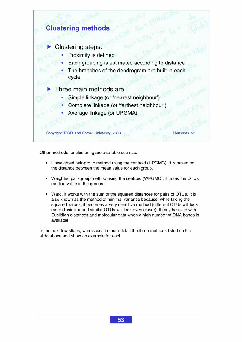
Clustering steps: • Proximity is defined • Each grouping is estimated according to distance• The branches of the dendrogram are built in each

cycle

Three main methods are:• Simple linkage (or ‘nearest neighbour’)• Complete linkage (or ‘farthest neighbour’)• Average linkage (or UPGMA)

Other methods for clustering are available such as:

• Unweighted pair-group method using the centroid (UPGMC). It is based on the distance between the mean value for each group.

• Weighted pair-group method using the centroid (WPGMC). It takes the OTUs’median value in the groups.

• Ward. It works with the sum of the squared distances for pairs of OTUs. It is also known as the method of minimal variance because, while taking the squared values, it becomes a very sensitive method (different OTUs will look more dissimilar and similar OTUs will look even closer). It may be used with Euclidian distances and molecular data when a high number of DNA bands is available.

In the next few slides, we discuss in more detail the three methods listed on the slide above and show an example for each.

54


Or ‘nearest neighbour’It minimizes the inter-group distance by taking the distance to the neighbour with the highest similarityIt works with regular and compact groups, but is highly influenced by distant individuals. This isinconvenient when there are different groups that are not well distributed in space

Group 1 Group 2

d(1,2)d(1,2) = minimum distance

between two OTUs

Simple linkage

55


Simple linkage: an example

00.400.600.28D

00.350.43C

00.30B

0A

DCBA(1) (2)

(3)

00.400.30AD

00.35C

0B

ADCB

0.100.200.300.400.50 0.0

A

D

B

C

(4)

00.35ADB

0C

ADBC

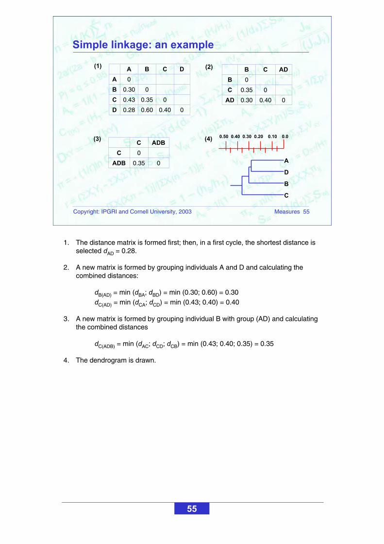
1. The distance matrix is formed first; then, in a first cycle, the shortest distance is selected dAD = 0.28.

2. A new matrix is formed by grouping individuals A and D and calculating the combined distances:

dB(AD) = min (dBA; dBD) = min (0.30; 0.60) = 0.30dC(AD) = min (dCA; dCD) = min (0.43; 0.40) = 0.40

3. A new matrix is formed by grouping individual B with group (AD) and calculating the combined distances

dC(ADB) = min (dAC; dCD; dCB) = min (0.43; 0.40; 0.35) = 0.35

4. The dendrogram is drawn.

56


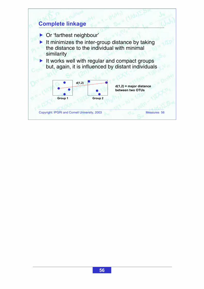
Or ‘farthest neighbour’It minimizes the inter-group distance by taking the distance to the individual with minimal similarityIt works well with regular and compact groups but, again, it is influenced by distant individuals

Group 1 Group 2

d(1,2)

d(1,2) = major distance

between two OTUs

Complete linkage

57


Complete linkage: an example

00.400.600.28D

00.350.43C

00.30B

0A

DCBA(1) (2)

(3) (4)

00.400.30BD

00.43C

0A

BDCA

0.100.200.300.400.500.60 0.0

A

D

B

C

00.40DB

0AC

DBAC

1. The distance matrix is formed first; then, in a first cycle, the longest distance is selected, dBD = 0.60.

2. A new matrix is formed by grouping individuals B and D and calculating the combined distances:

dA(BD) = max(dBA; dAD) = max(0.30; 0.28) = 0.30dC(BD) = max(dCB; dCD) = max(0.35; 0.40) = 0.40

3. The new matrix is formed with groups AC and BD, and the combined distances calculated:

d(AC)(DB) = max (dAD; dAB; dCD; dCB) = max (0.28; 0.30; 0.40; 0.35) = 0.40

4. The dendrogram is drawn.

58


Or ‘unweighted pair-group method using the arithmetic average’ (UPGMA)It minimizes the inter-group distance by taking the average pairwise distance among all individuals of the sampleMost used method

d(1i ,2j) = average distance

between OTUi and OTUj of

groups 1 and 2

Group 1 Group 2

Average linkage

59


Average linkage: an example

00.400.600.28D

00.350.43C

00.30B

0A

DCBA(1) (2)

(3) (4) 0.10.20.30.40.5 0.0

B

D

A

C

00.4150.45AD

00.35C

0B

ADCB

00.42AD

0BC

ADBC

1. The distance matrix is formed first; then, in a first cycle, the shortest distance is selected, dAD = 0.28

2. Next, a matrix is formed by grouping individual A with D and calculating the combined distances:

dB(AD) = (dBA + dBD)/2 = (0.30 + 0.60)/2 = 0.45dC(AD) = (dCA + dCD)/2 = (0.43 + 0.40)/2 = 0.415

3. A new matrix is formed by grouping the individuals with the shortest distance B with C, and calculating the combined distances:

d(AD) (BC) = (dAB + dAC + dBD + dBC)/4 = (0.30 + 0.43 + 0.60 + 0.35)/4 = 0.42

60


First, gather knowledge of the species under study such as its diversity, reproduction system, ploidy number and levels of heterozygosity

Carefully select the genetic characters to analyse

Test different clustering methodologies and assess the level of agreement obtained with each of them

Choosing a clustering method

In addition, it will always be important to combine as much information as possible. An example may be found in Appendix 8 (click here), in which both morphological and molecular data are available, and the use of separate data sets is compared with the use of combined data.

61


External validation

Internal validation

Relative validation

Bootstrapping

Validating the clustering analysis

External validation:The matrix distance is compared with other information not used in the grouping calculations (e.g. genealogy).

Internal validation:This technique quantifies the distortion due to the grouping method used. It builds a new similarity or distance matrix, the ‘co-phenetic matrix’, directly from the dendrogram. Validation is calculated by means of a correlation coefficient between similarity or distance data from the original matrix and those from the new co-phenetic matrix. Whether the original distances are maintained is assessed after the grouping exercise (Sokal and Rohlf, 1994).

Relative validation:Similarity between methods is compared.

Bootstrapping:This is a re-sampling method by replacement with the same data matrix. It allows calculation of standard deviations and variances, and is useful for those situations in which the number of samples or resources (e.g. time, budget) is limited.

Examples of applying the co-phenetic correlation and bootstrapping methods are shown next.

Reference

Sokal, R. and J. Rohlf. 1994. Biometry: The Principles and Practice of Statistics in Biological Research (3rd edn.). Freeman & Co, NY.

62


00.400.600.28D

00.350.43C

00.30B

0A

DCBA

Original distance matrix

Dendrogram

0.100.200.300.400.500.60 0.0

00.430.430.28D

00.350.43C

00.43B

0A

DCBA

Co-phenetic matrix

B

D

A

C

0.280.350.43

Co-phenetic correlation =

0.5557

Co-phenetic correlation: an example

To construct the co-phenetic matrix, we look at the dendrogram previously built withthe original matrix (this example comes from slide 58). We see that the distance between D and C in the dendrogram is 0.43, so we fill that cell in the co-phenetic matrix. Distance between B and C is 0.35, and so on.

Calculations for the co-phenetic correlation are based on the correlation coefficient:

r = ( XiYi - Xi Yi/n)/SXiSYi

Where,Xi and Yi are the similarity or distance values of the original and co-phenetic matrix, respectivelySXi and SYi are the standard deviations for each variable

If the correlation value is high, we can conclude that the dendrogram does indeed reflect the distances in the original matrix and that therefore there is no distortion due to the grouping method. In the above example, we obtained a value 0.5557. This is an average value that could indicate that the dendrogram distances do not reflect the distance data in the original matrix, and so distortion exists because of the method used. However, in building the example, we used very few data; nor were they the real results of an experiment, thus explaining the value obtained.

63


1000L5

0011L4

1101L3

1010L2

1001L1

P4P3P2P1

Data matrix

Similarity matrix

A P1 P2 P3 P4

Gel

B

C

DE

(1) (2)

(3)

Bootstrapping validation: an example

10.4000.2000.400P4

10.4000.600P3

10.400P2

1P1

P4P3P2P1


In the gel above (top left corner), we have 4 individuals (Pi) and 5 loci (Lj). We will suppose we perform the validation in three samples with replacement.

First, we score the marker data in the individuals (data matrix) and then, we calculate the average similarity (simple matching) and its interval.

64


10.400 ± 0.2000.200 ± 0.0000.533 ± 0.115P4

10.400 ± 0.2000.600 ± 0.000P3

10.267 ± 0.115P2

1P1

P4P3P2P1

Average similarity matrix

with standard deviations

Dendrogram before replacement Dendrogram with replacement

Bootstrapping validation: an example (continued)

1

0.25 0.44 0.63 0.81 1.00

3

2

4

0.11 0.33 0.56 0.78 1.00

1

3

4

2

For each individual, the value for each locus is taken, one by one, with replacement and a sample formed of equal size to the number of loci. The possibility exists that a locus is selected one or more times. For the example:

M1: L1 L1 L2 L3 L5 (locus L4 was not drawn)M2: L1 L2 L3 L4 L3

M3: L3 L1 L5 L2 L4

In each sample a similarity matrix is calculated.

Average similarities and their standard deviations are estimated for each individual pair (1 & 2, 1 & 3, 2 & 3, and so on), and the average similarity matrix is created.

A new dendrogram is built, using the average similarity matrix.

For real situations, more than 100 replacement samples should be created.

65


Ordination is the arrangement or ‘ordering’ of sample units along coordinate systems

The purpose of ordination, as well as classification methods, is to interpret patterns in the composition of samples

Displaying relationships: ordination

Ordination is a multivariate method that complements clustering, and is usually considered to be an approach that is closer to biological reality.

With ordination methods, we want to represent the relationships of samples in a simple way by reducing the real situation to a ‘low dimensional space’ (Gauch, 1982). In doing so, the sample’s composition is studied as a whole, the statistical power of the analysis is improved because redundancy is somehow eliminated or reduced, and the relative importance of different gradients can be determined. Most of all, we get graphical representations that help us intuitively interpret the relationships of the different groups of samples.

In principle, ordination is both an exploratory and hypothesis-testing tool. In any case, the results obtained with ordination methods should always be contrasted with the available knowledge of the sample being studied and as much as possible with additional information related to the biological question being addressed in the research.

Reference

Gauch, H.G., Jr. 1982. Multivariate Analysis and Community Structure.Cambridge University Press, UK.

66


Principal coordinates analysis (PCoA)

Nonmetric multidimensional scaling (NMDS)

Correspondence analysis (CA)

Useful ordination methods for molecular marker data

Many ordination techniques exist—some are based on distance data or on the calculations of the so-called Eigenvalues (the sum of all variances for each character in each component). However, those techniques based on continuous variables (e.g. principal component analysis or PCA) are not appropriate for use with marker data. Hence, we discuss only briefly the three listed in the slide above. More details on the basics of these methods would require a deeper mathematical understanding of the algorithms involved than what we expect from the average user of this module. We therefore encourage our readers who want to know more about these methods to search for ordination methods through the Web. For an overview, check the site <http://www.okstate.edu/artsci/botany/ordinate/overview.htm>

Principal coordinates analysis (PCoA) attempts to represent distances between samples and may accommodate matrices from different dissimilarity measures. It maximizes the linear correlation between sample distances. When used with Euclidean distances, the results are identical to PCA.

Nonmetric multidimensional scaling (NMDS) works by maximizing the rank order correlation and attempting to find the best shape to accommodate the data. This technique uncovers the basic configuration from the dissimilarity sample matrix. With NMDS, only the pattern of points is relevant, not the origin, and the representation may be rotated.

Correspondence analysis (CA) repeats the averages of sample scores and finds spots where all samples falling in the same spot are as similar as possible and, simultaneously, samples at different spots are as different as possible.

67


Appendices

2. Analysis of molecular variance: example 1

3. Analysis of molecular variance: example 2

4. Geometric distance

5. Transforming data from quantitative variables: an example

6. Applying the simple matching coefficient for morphological characters (categorical variables)

7. Calculating Nei’s genetic distance

8. Morphological and molecular similarities

68


The analysis of genetic diversity and structure of populations involves:

• The quantification of diversity and the relationships within and between populations and/or individuals

• The display of relationships

Molecular data are usually handled as binary data

Molecular data can be usefully complemented with morphological or evaluation data. To do so, there types of variables can be transformed to binary variables

In summary

69


The basic steps involved in measuring genetic diversityThe major ways to describe genetic diversity within and among populationsThe correct selection of distance calculation to assess relationships in the sample of interestThe differences between alternative clustering methodsThe options available to validate grouping The basic notions underlying the concept of ordinationThe similarities and differences between clustering and ordination

By now you should know …

70


References

Cavalli–Sforza, L.L. and W.F. Bodmer. 1981. Genética de las Poblaciones Humanas. Ed. Omega, Barcelona.

García, J.A., M.C. Duque, J. Tohme, S. Xu and M. Levy. 1995. SAS for Classification Analysis; Agrobiotecnology Course, October 1995. Working document. Centro Internacional de Agricultura Tropical (CIAT), Cali, Colombia.

Gauch, H.G., Jr. 1982. Multivariate Analysis and Community Structure. Cambridge University Press, UK.

Karp, A., P.G. Isaac and D.S. Ingram. 1998. Molecular Tools for Screening Biodiversity: Plants and Animals. Chapman & Hall, London.

Lynch, M. and B.G. Milligan. 1994. Analysis of population genetic structure with RAPD markers. Mol. Ecol. 3:91-99.

Sokal, R. and J. Rohlf. 1994. Biometry: The Principles and Practice of Statistics in Biological Research (3rd edn.). Freeman & Co, NY.

71


Software programs for analysing genetic diversity

Glossary

Next

Copyright: IPGRI and Cornell University, 2003 Measures 1 · slide, Ind 1, Ind 2, … may represent,...

Documents

Transcript of Copyright: IPGRI and Cornell University, 2003 Measures 1 · slide, Ind 1, Ind 2, … may represent,...