Copyright (c) Bani K. Mallick1 STAT 651 Lecture #16.
35
Copyright (c) Bani K. Mal lick 1 STAT 651 Lecture #16
-
date post
21-Dec-2015 -
Category
Documents
-
view
216 -
download
1
Transcript of Copyright (c) Bani K. Mallick1 STAT 651 Lecture #16.

Copyright (c) Bani K. Mallick 1
STAT 651
Lecture #16

Copyright (c) Bani K. Mallick 2
Topics in Lecture #16 Inference about two population
proportions

Copyright (c) Bani K. Mallick 3
Book Sections Covered in Lecture #16
Chapter 10.3
Copyright (c) Bani K. Mallick 4
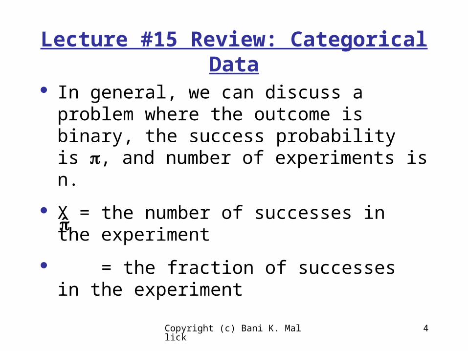
Lecture #15 Review: Categorical Data
In general, we can discuss a problem where the outcome is binary, the success probability is , and number of experiments is n.
X = the number of successes in the experiment
= the fraction of successes in the experiment

Copyright (c) Bani K. Mallick 5
Lecture #15 Review: Categorical Data
The number of success X in n experiments each with probability of success is called a binomial random variable
There is a formula for this:
Pr(X = k) =
0! = 1, 1! = 1, 2! = 2 x 1 = 2, 3! = 3 x 2 x 1 = 6, 4! = 4 x 3 x 2 x 1 = 24, etc.
k n kn!(1 )
k! (n-k)!
Copyright (c) Bani K. Mallick 6
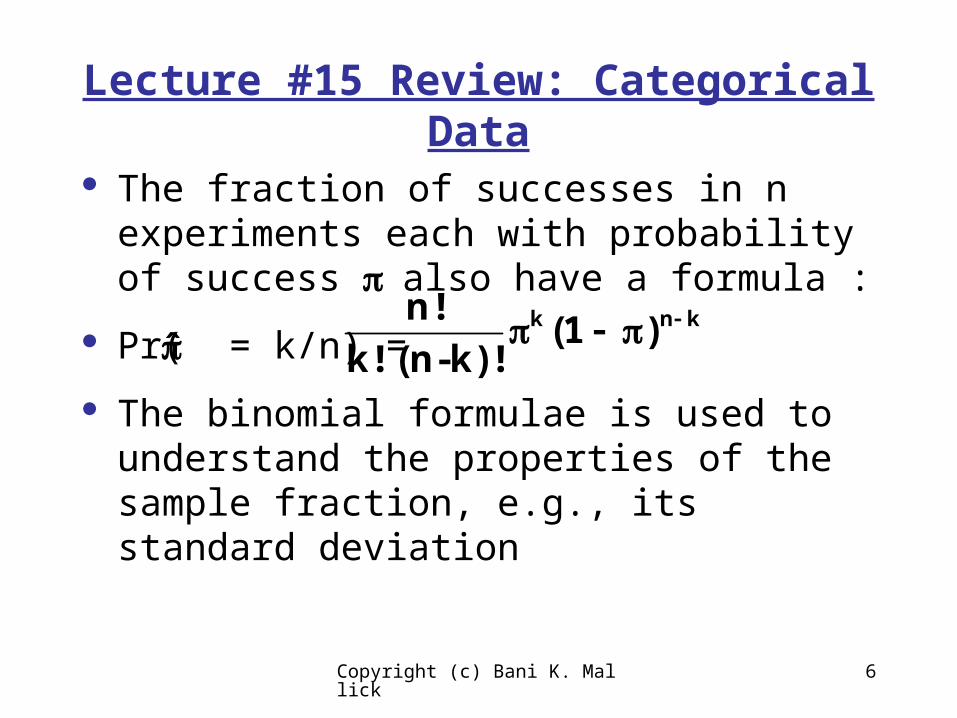
Lecture #15 Review: Categorical Data
The fraction of successes in n experiments each with probability of success also have a formula :
Pr( = k/n) =
The binomial formulae is used to understand the properties of the sample fraction, e.g., its standard deviation
k n kn!(1 )
k! (n-k)!

Copyright (c) Bani K. Mallick 7
Lecture #15 Review:
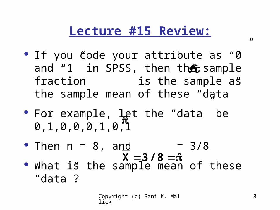
If you code your attribute as “0” and “1” in SPSS, then the sample fraction is the sample as the sample mean of these “data”
For example, let the “data” be 0,1,0,0,0,1,0,1
Then n = 8, and = 3/8
What is the sample mean of these data?
Copyright (c) Bani K. Mallick 8
Lecture #15 Review:
If you code your attribute as “0” and “1” in SPSS, then the sample fraction is the sample as the sample mean of these “data”
For example, let the “data” be 0,1,0,0,0,1,0,1
Then n = 8, and = 3/8
What is the sample mean of these “data”?
X 3/ 8 ˆ
Copyright (c) Bani K. Mallick 9
Lecture #15 Review: Categorical Data
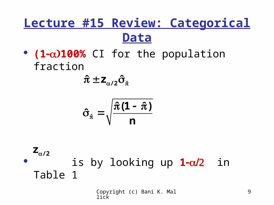
(1100% CI for the population fraction
is by looking up 1 in Table 1
/ 2 ˆzˆ ˆ
ˆ
(1 )ˆ ˆˆ
n
/ 2z

Copyright (c) Bani K. Mallick 10
Lecture #15 Review: Sample Size Calculations
If you want an (1100% CI interval to be
you should set
E 2
/ 2 2
(1 )n z
E

Copyright (c) Bani K. Mallick 11
Lecture #15 Review: Sample Size Calculations
The small problem is that you do not know . You have two choices:
Make a guess for
Set = 0.50 and calculate (most conservative, since it results in largest sample size)
2/ 2 2
(1 )n z
E
Copyright (c) Bani K. Mallick 12
Comparison of Two Population Proportions
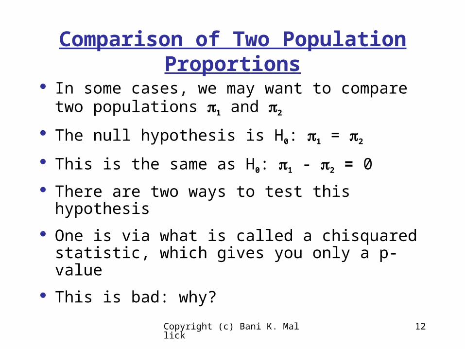
In some cases, we may want to compare two populations 1 and 2
The null hypothesis is H0: 1 = 2
This is the same as H0: 1 - 2 = 0
There are two ways to test this hypothesis
One is via what is called a chisquared statistic, which gives you only a p-value
This is bad: why?
Copyright (c) Bani K. Mallick 13
Comparison of Two Population Proportions
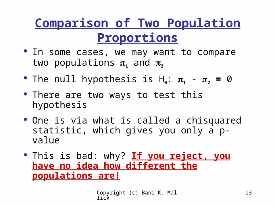
In some cases, we may want to compare two populations 1 and 2
The null hypothesis is H0: 1 - 2 = 0
There are two ways to test this hypothesis
One is via what is called a chisquared statistic, which gives you only a p-value
This is bad: why? If you reject, you have no idea how different the populations are!

Copyright (c) Bani K. Mallick 14
Comparison of Two Population Proportions
The null hypothesis is H0: 1 - 2 = 0
The other way is to form a CI for the difference in population proportions 1 - 2
The estimate of this difference is simply the difference in the sample fractions:1 2ˆ ˆ
Copyright (c) Bani K. Mallick 15
Comparison of Two Population Proportions
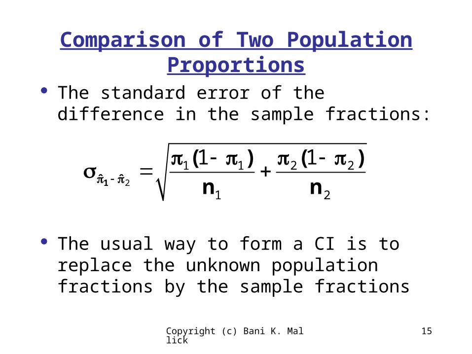
The standard error of the difference in the sample fractions:
The usual way to form a CI is to replace the unknown population fractions by the sample fractions
2
1 1 2 2
1 2
1 1
1ˆ ˆ
( ) ( )n n
Copyright (c) Bani K. Mallick 16
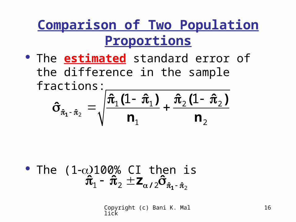
Comparison of Two Population Proportions
The estimated standard error of the difference in the sample fractions:
The (1100% CI then is
2
1 1 2 2
1 2
1 1
1ˆ ˆ
( ) ( )ˆ ˆ ˆ ˆˆ
n n
21 2 2 1/ ˆ ˆzˆ ˆ ˆ

Copyright (c) Bani K. Mallick 17
Comparison of Two Population Proportions: Boxers versus Brief Most books force you to compute this
by hand
For female preferences in men:
For male preferences:
Think the populations are different?
1 1177 0 7345 n , .
2 2188 0 4681 n , .
1 2 0 2664 .ˆ ˆ
Copyright (c) Bani K. Mallick 18
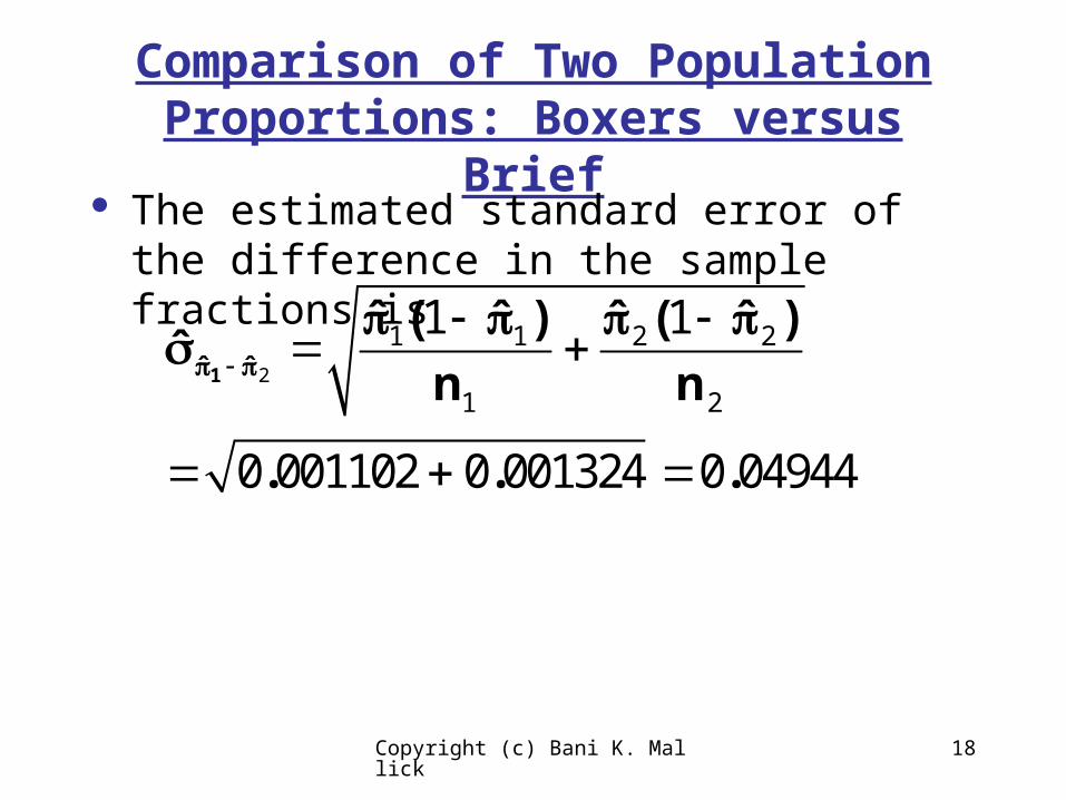
Comparison of Two Population Proportions: Boxers versus Brief The estimated standard error of the
difference in the sample fractions is
2
1 1 2 2
1 2
1 1
0 001102 0 001324 0 04944
1ˆ ˆ
( ) ( )ˆ ˆ ˆ ˆˆ
n n
. . .
Copyright (c) Bani K. Mallick 19
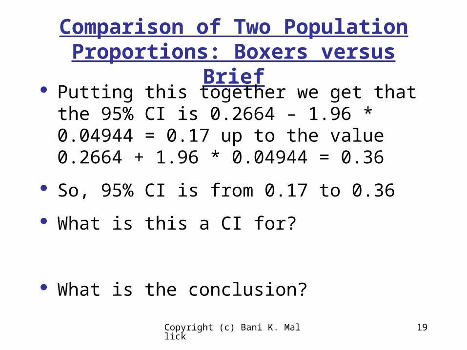
Comparison of Two Population Proportions: Boxers versus Brief Putting this together we get that the
95% CI is 0.2664 – 1.96 * 0.04944 = 0.17 up to the value 0.2664 + 1.96 * 0.04944 = 0.36
So, 95% CI is from 0.17 to 0.36
What is this a CI for?
What is the conclusion?

Copyright (c) Bani K. Mallick 20
Comparison of Two Population Proportions: Boxers versus Brief 95% CI is from 0.17 to 0.36
What is this a CI for? The difference in population fractions of preferring boxers is from 0.17 to 0.36
What is the conclusion? More females prefer men to wear boxers than do males, by 17% to 36%
Copyright (c) Bani K. Mallick 21
Comparison of Two Population Proportions:
Remarkably, but perhaps not surprisingly, you do not have to compute these confidence intervals by hand!
The idea: simply pretend, and I do mean pretend, that the binary outcomes are real numbers and run your ordinary t-test CI, unequal variance line
The results will be slightly different from your hand calculations, but actually a bit more accurate
Copyright (c) Bani K. Mallick 22
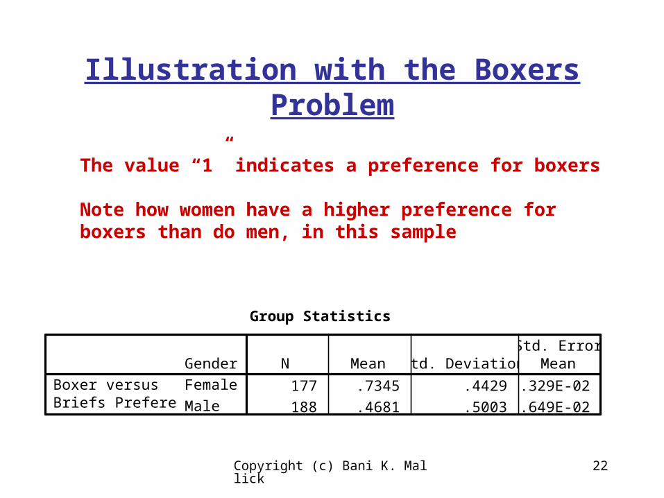
Illustration with the Boxers Problem
Group Statistics
177 .7345 .4429 3.329E-02
188 .4681 .5003 3.649E-02
GenderFemale
Male
Boxer versusBriefs Preference
N Mean Std. DeviationStd. Error
Mean
The value “1” indicates a preference for boxers
Note how women have a higher preference for boxers than do men, in this sample

Copyright (c) Bani K. Mallick 23
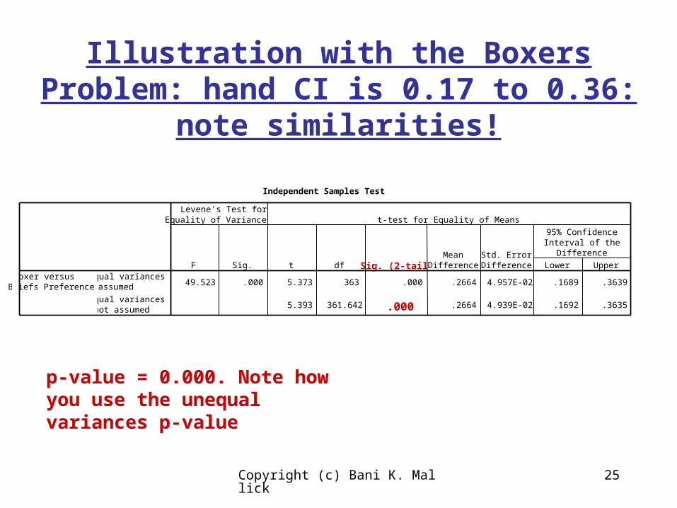
Illustration with the Boxers Problem
Independent Samples Test
49.523 .000 5.373 363 .000 .2664 4.957E-02 .1689 .3639
5.393 361.642 .000 .2664 4.939E-02 .1692 .3635
Equal variancesassumed
Equal variancesnot assumed
Boxer versusBriefs Preference
F Sig.
Levene's Test forEquality of Variances
t df Sig. (2-tailed)Mean
DifferenceStd. ErrorDifference Lower Upper
95% ConfidenceInterval of the
Difference
t-test for Equality of Means

Copyright (c) Bani K. Mallick 24
Illustration with the Boxers Problem
Independent Samples Test
49.523 .000 5.373 363 .000 .2664 4.957E-02 .1689 .3639
5.393 361.642 .000 .2664 4.939E-02 .1692 .3635
Equal variancesassumed
Equal variancesnot assumed
Boxer versusBriefs Preference
F Sig.
Levene's Test forEquality of Variances
t df Sig. (2-tailed)Mean
DifferenceStd. ErrorDifference Lower Upper
95% ConfidenceInterval of the
Difference
t-test for Equality of Means
Difference in sample means = 0.2664
Standard error of this difference = 0.04939
Copyright (c) Bani K. Mallick 25
Illustration with the Boxers Problem: hand CI is 0.17 to 0.36: note
similarities!
Independent Samples Test
49.523 .000 5.373 363 .000 .2664 4.957E-02 .1689 .3639
5.393 361.642 .000 .2664 4.939E-02 .1692 .3635
Equal variancesassumed
Equal variancesnot assumed
Boxer versusBriefs Preference
F Sig.
Levene's Test forEquality of Variances
t df Sig. (2-tailed)Mean
DifferenceStd. ErrorDifference Lower Upper
95% ConfidenceInterval of the
Difference
t-test for Equality of Means
p-value = 0.000. Note how you use the unequal variances p-value
Copyright (c) Bani K. Mallick 26
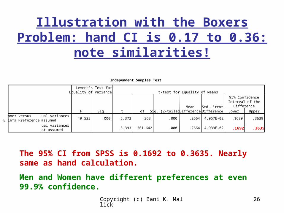
Illustration with the Boxers Problem: hand CI is 0.17 to 0.36: note
similarities!
Independent Samples Test
49.523 .000 5.373 363 .000 .2664 4.957E-02 .1689 .3639
5.393 361.642 .000 .2664 4.939E-02 .1692 .3635
Equal variancesassumed
Equal variancesnot assumed
Boxer versusBriefs Preference
F Sig.
Levene's Test forEquality of Variances
t df Sig. (2-tailed)Mean
DifferenceStd. ErrorDifference Lower Upper
95% ConfidenceInterval of the
Difference
t-test for Equality of Means
The 95% CI from SPSS is 0.1692 to 0.3635. Nearly same as hand calculation.
Men and Women have different preferences at even 99.9% confidence.

Copyright (c) Bani K. Mallick 27
US Availability and Rating: Are Better Beers More Widely
Available?
Group Statistics
11 0.45 .52 .16
24 0.75 .44 9.03E-02
Very Good versus OtherVery Good
Fair or Good
Availability in the U.S.N Mean Std. Deviation
Std. ErrorMean
With the “data” coded as 0 and 1, this means that in the sample, 45% of the very good beers were widely available
The “data” are coded as 0 = not widely available 1 = widely available

Copyright (c) Bani K. Mallick 28
US Availability and Rating: Are Better Beers More Widely
Available?
Group Statistics
11 0.45 .52 .16
24 0.75 .44 9.03E-02
Very Good versus OtherVery Good
Fair or Good
Availability in the U.S.N Mean Std. Deviation
Std. ErrorMean
With the “data” coded as 0 and 1, this means that in the sample, 75% of the fair/good beers were widely available

Copyright (c) Bani K. Mallick 29
US Availability and Rating: Are Better Beers More Widely
Available?
Independent Samples Test
3.169 .084 -1.734 33 .092 -.30 .17 -.64 5.12E-02
-1.628 16.864 .122 -.30 .18 -.68 8.77E-02
Equal variancesassumed
Equal variancesnot assumed
Availability in the U.S.F Sig.
Levene's Test forEquality of Variances
t df Sig. (2-tailed)Mean
DifferenceStd. ErrorDifference Lower Upper
95% ConfidenceInterval of the
Difference
t-test for Equality of Means
This is the p-value for the hypothesis that the two population fractions are the same
Copyright (c) Bani K. Mallick 30
Comparison of Two Population Proportions:
Note that the p-values were > 0.10
What does this mean?

Copyright (c) Bani K. Mallick 31
Comparison of Two Population Proportions:
Note that the p-values were > 0.10
What does this mean?
There is no evidence that those beers which are very good have any more or less national availability than those which are good or fair
Copyright (c) Bani K. Mallick 32
Construction Example
The construction example was based on a survey made available to me.
I will look at the percentages of males sampled in Texas and in states outside of Texas
If these were random samples, they would be a measure of how different states are in their gender distributions in the construction industry

Copyright (c) Bani K. Mallick 33
Construction Data: Gender Differences by Texas or Not
(1 = male)
Group Statistics
274 .86 .34 2.07E-02
173 .26 .44 3.35E-02
State: Texas or NotOutside Texas
Texas
SexN Mean Std. Deviation
Std. ErrorMean
Something strange: 86% of the sample outside Texas is male26% of the sample in Texas is male

Copyright (c) Bani K. Mallick 34
Construction Data: Gender Differences by Texas or Not
(1 = male)
Something strange: 86% of the sample outside Texas is male26% of the sample in Texas is male
Not surprising: p-value = 0.000
Independent Samples Test
43.713 .000 16.260 445 .000 .60 3.72E-02 .53 .68
15.379 300.960 .000 .60 3.93E-02 .53 .68
Equal variancesassumed
Equal variancesnot assumed
SexF Sig.
Levene's Test forEquality of Variances
t df Sig. (2-tailed)Mean
DifferenceStd. ErrorDifference Lower Upper
95% ConfidenceInterval of the
Difference
t-test for Equality of Means

Copyright (c) Bani K. Mallick 35
Comparison of Two Population Proportions:
Please study the slides for the next lecture before coming to class
The material is somewhat difficult, and if you do not look at the slides and try to understand them, you will find my lecture all but impossible to understand.