Copyright (c) Bani K. Mallick1 STAT 651 Lecture #20.
43
Copyright (c) Bani K. Mal lick 1 STAT 651 Lecture #20
-
date post
21-Dec-2015 -
Category
Documents
-
view
213 -
download
0
Transcript of Copyright (c) Bani K. Mallick1 STAT 651 Lecture #20.

Copyright (c) Bani K. Mallick 1
STAT 651
Lecture #20
Copyright (c) Bani K. Mallick 2
Topics in Lecture #20 Outliers and Leverage
Cook’s distance

Copyright (c) Bani K. Mallick 3
Book Chapters in Lecture #20 Small part of Chapter 11.2

Copyright (c) Bani K. Mallick 4
Relevant SPSS Tutorials Regression diagnostics
Diagnostics for problem points
Copyright (c) Bani K. Mallick 5
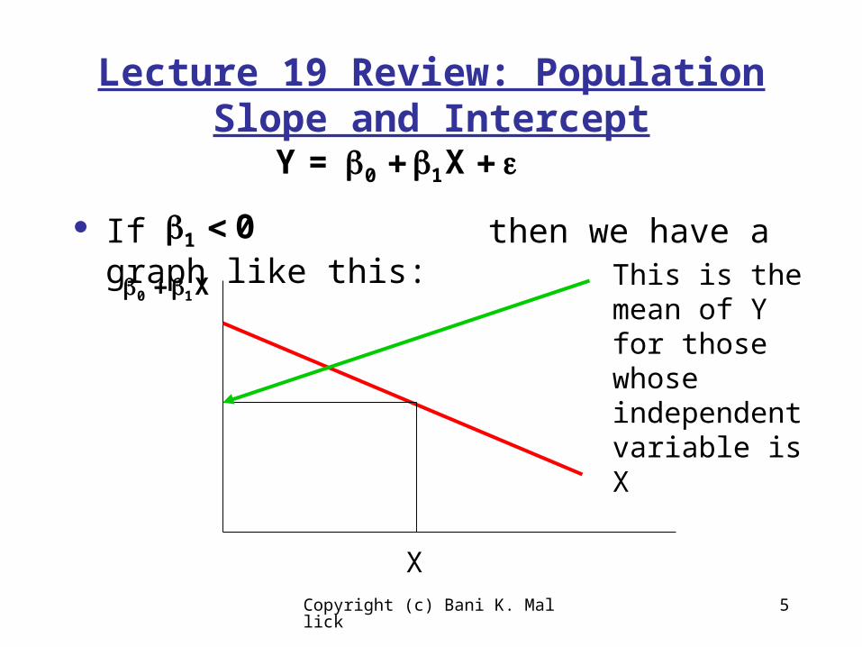
Lecture 19 Review: Population Slope and Intercept
If then we have a graph like this:
0 1Y = X
1 0
X
0 1X This is the mean of Y for those whose independent variable is X

Copyright (c) Bani K. Mallick 6
Lecture 19 Review: Population Slope and Intercept
If then we have a graph like this:
0 1Y = X
1 0
X
0 1 X Note how the mean of Y does not depend on X: Y and X are independent

Copyright (c) Bani K. Mallick 7
Lecture 19 Review: Linear Regression
If then Y and X are independent
So, we can test the null hypothesis that Y and X are independent by testing
The p-value in regression tables tests this hypothesis
0 1Y = X
1 0
0H :
0 1H : 0
Copyright (c) Bani K. Mallick 8
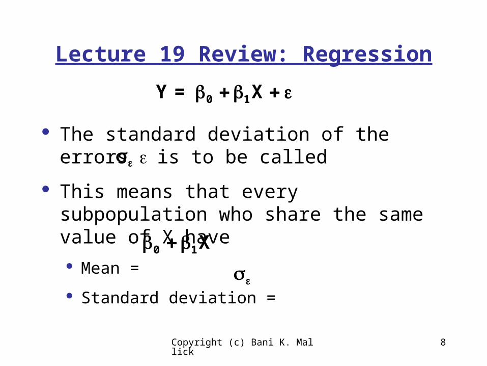
Lecture 19 Review: Regression
The standard deviation of the errors is to be called
This means that every subpopulation who share the same value of X have Mean =
Standard deviation =
0 1Y = X
0 1X
Copyright (c) Bani K. Mallick 9
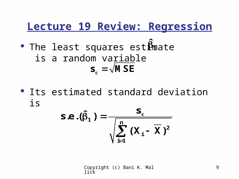
Lecture 19 Review: Regression
The least squares estimate is a random variable
Its estimated standard deviation is
1̂
1 n2
ii 1
sˆs.e.( )
(X X)
s MSE
Copyright (c) Bani K. Mallick 10
Lecture 19 Review: Regression
The (1100% Confidence interval for the population slope is
1 / 2 1ˆ ˆt (n 2)se( )

Copyright (c) Bani K. Mallick 11
Lecture 19 Review: Residuals
You can check the assumption that the errors are normally distributed by constructing a q-q plot of the residuals

Copyright (c) Bani K. Mallick 12
Leverage and Outliers
Outliers in Linear Regression are difficult to diagnose
They depend crucially on where X is
* **
*
*
A boxplot of Y would think this is an outlier, when in reality it fits the line quite well
Copyright (c) Bani K. Mallick 13
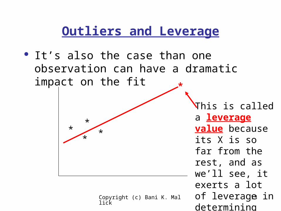
Outliers and Leverage
It’s also the case than one observation can have a dramatic impact on the fit
**
**
*
This is called a leverage value because its X is so far from the rest, and as we’ll see, it exerts a lot of leverage in determining the line
Copyright (c) Bani K. Mallick 14
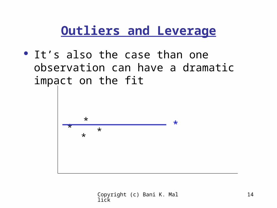
Outliers and Leverage
It’s also the case than one observation can have a dramatic impact on the fit
**
**
*

Copyright (c) Bani K. Mallick 15
Outliers and Leverage
It’s also the case than one observation can have a dramatic impact on the fit
**
**
*
Copyright (c) Bani K. Mallick 16
Outliers and Leverage
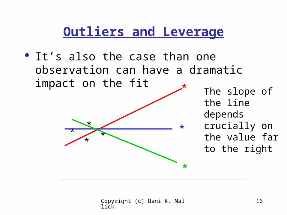
It’s also the case than one observation can have a dramatic impact on the fit
**
**
*
*
*
The slope of the line depends crucially on the value far to the right
Copyright (c) Bani K. Mallick 17
Outliers and Leverage
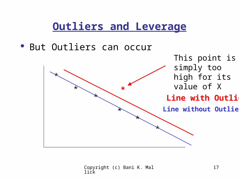
But Outliers can occur
*
**
**
*
*
This point is simply too high for its value of XLine with Outlier
Line without Outlier

Copyright (c) Bani K. Mallick 18
Outliers and Leverage
A leverage point is an observation with a value of X that is outlying among the X values
An outlier is an observation of Y that seems not to agree with the main trend of the data
Outliers and leverage values can distort the fitted least squares line
It is thus important to have diagnostics to detect when disaster might strike
Copyright (c) Bani K. Mallick 19
Outliers and Leverage
We have three methods for diagnosing high leverage values and outliers
Leverage plots: For a single X, these are basically the same as boxplots of the X-space (leverage)
Cook’s distance (measures how much the fitted line changes if the observation is deleted)
Residual Plots

Copyright (c) Bani K. Mallick 20
Outliers and Leverage
Leverage plots: You plot the leverage against the observation number (first observation in your data file = #1, second = #2, etc.)
Leverage for observation j is defined as
In effect, you measure the distance of an observation to its mean in relation to the total distance of the X’s
2
j
jj 2n
ii 1
X Xh
X X
Copyright (c) Bani K. Mallick 21
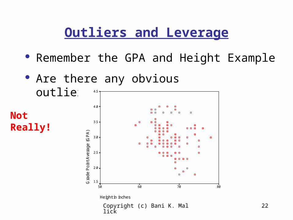
Outliers and Leverage
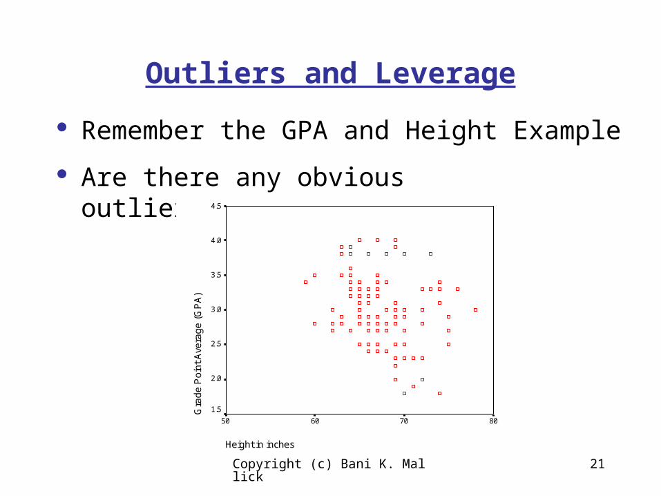
Remember the GPA and Height Example
Are there any obvious outliers/leverage points?
Height in inches
80706050
Gra
de
Po
int
Ave
rag
e (
GP
A)
4.5
4.0
3.5
3.0
2.5
2.0
1.5
Copyright (c) Bani K. Mallick 22
Outliers and Leverage
Remember the GPA and Height Example
Are there any obvious outliers/leverage points?
Height in inches
80706050
Gra
de
Po
int
Ave
rag
e (
GP
A)
4.5
4.0
3.5
3.0
2.5
2.0
1.5
Not Really!
Copyright (c) Bani K. Mallick 23
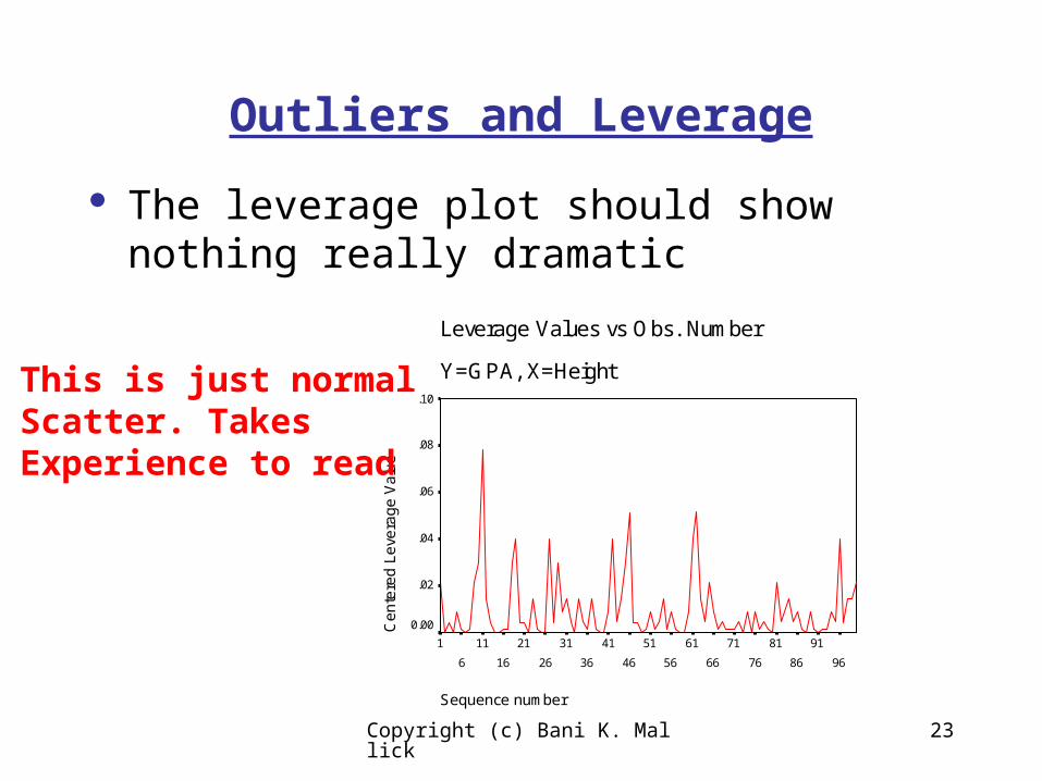
Outliers and Leverage
The leverage plot should show nothing really dramatic
Leverage Values vs Obs. Number
Y=GPA, X=Height
Sequence number
96
91
86
81
76
71
66
61
56
51
46
41
36
31
26
21
16
11
6
1
Ce
nte
red
Le
vera
ge
Va
lue
.10
.08
.06
.04
.02
0.00
This is just normalScatter. Takes Experience to read
Copyright (c) Bani K. Mallick 24
Outliers and Leverage
The Cook’s Distance for an observation is defined as follows
Compute the fitted values with all the data
Compute the fitted values with observation j deleted
Compute the sum of the squared differences
Measures how much the line changes when an observation is deleted
Copyright (c) Bani K. Mallick 25
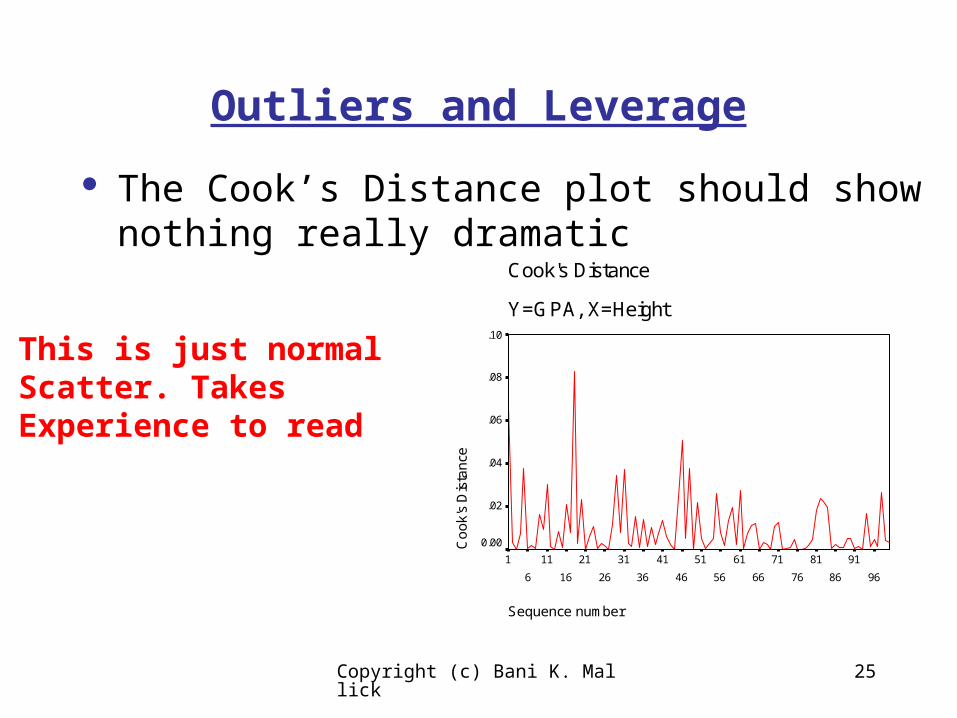
Outliers and Leverage
The Cook’s Distance plot should show nothing really dramatic
This is just normalScatter. Takes Experience to read
Cook's Distance
Y=GPA, X=Height
Sequence number
96
91
86
81
76
71
66
61
56
51
46
41
36
31
26
21
16
11
6
1
Co
ok'
s D
ista
nce
.10
.08
.06
.04
.02
0.00
Copyright (c) Bani K. Mallick 26
Outliers and Leverage
The residual plot is a plot of the residuals (on the y-axis) against the predicted values (on the x-axis)
You should look for values which seem quite extreme

Copyright (c) Bani K. Mallick 27
Outliers and Leverage
The residual plot should show nothing really dramatic
This is just normalScatter. No massiveOutliers. Takes Experience to read
Residual Plot
Y=GPA, X=Height
Unstandardized Predicted Value
3.43.23.02.82.6
Un
sta
nd
ard
ize
d R
esi
du
al
1.5
1.0
.5
0.0
-.5
-1.0
-1.5

Copyright (c) Bani K. Mallick 28
Outliers and Leverage
A much more difficult example occurs with the stenotic kids
Coefficientsa
.167 .079 2.099 .041 .007 .326
.319 .059 .591 5.390 .000 .200 .438
(Constant)
Body Surface Area
Model1
B Std. Error
UnstandardizedCoefficients
Beta
Standardized
Coefficients
t Sig. Lower Bound Upper Bound
95% Confidence Interval for B
Dependent Variable: Log(1+Aortic Valve Area)a.
Copyright (c) Bani K. Mallick 29
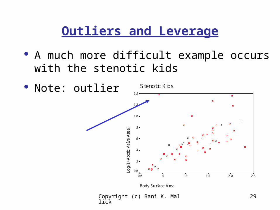
Outliers and Leverage
A much more difficult example occurs with the stenotic kids
Note: outlier? Stenotic Kids
Body Surface Area
2.52.01.51.0.50.0
Lo
g(1
+A
ort
ic V
alv
e A
rea
)
1.4
1.2
1.0
.8
.6
.4
.2
0.0
Copyright (c) Bani K. Mallick 30
Outliers and Leverage
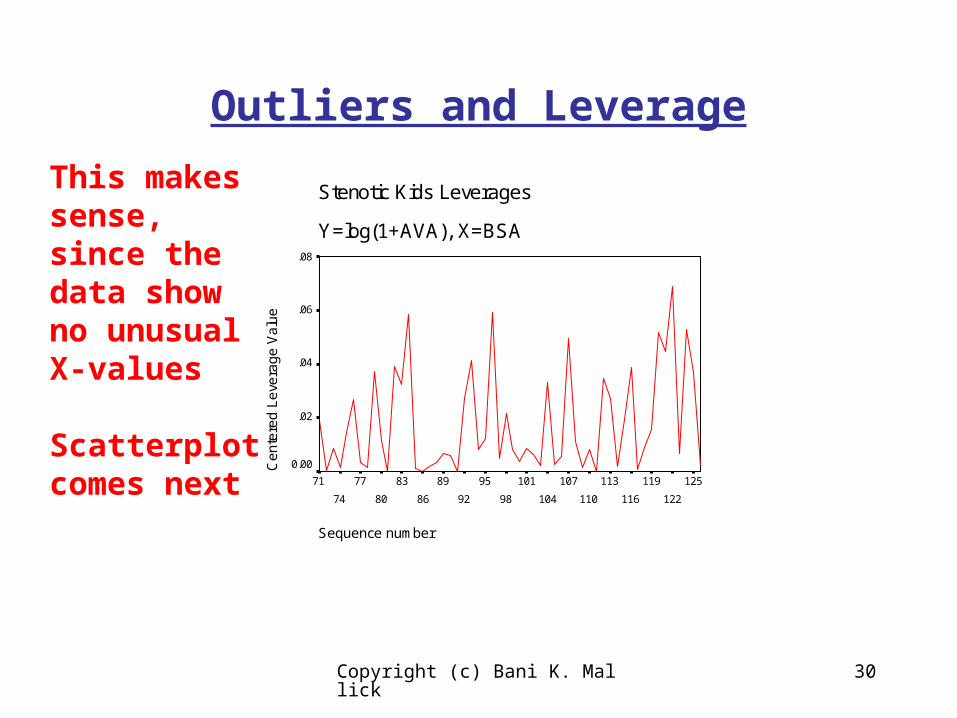
Stenotic Kids Leverages
Y=log(1+AVA), X=BSA
Sequence number
125
122
119
116
113
110
107
104
101
98
95
92
89
86
83
80
77
74
71
Ce
nte
red
Le
vera
ge
Va
lue
.08
.06
.04
.02
0.00
This makes sense, since the data show no unusual X-values
Scatterplot comes next

Copyright (c) Bani K. Mallick 31
Outliers and Leverage
A much more difficult example occurs with the stenotic kids
Note: outlier? Stenotic Kids
Body Surface Area
2.52.01.51.0.50.0
Lo
g(1
+A
ort
ic V
alv
e A
rea
)
1.4
1.2
1.0
.8
.6
.4
.2
0.0

Copyright (c) Bani K. Mallick 32
Outliers and Leverage
Wow! Cook's Distances, Stenotic Kids
Y=log(1+AVA), X=BSA
Sequence number
125
122
119
116
113
110
107
104
101
98
95
92
89
86
83
80
77
74
71
Co
ok'
s D
ista
nce
.7
.6
.5
.4
.3
.2
.1
0.0
This is a case that there is a noticeable outlier, but not too high leverage
Copyright (c) Bani K. Mallick 33
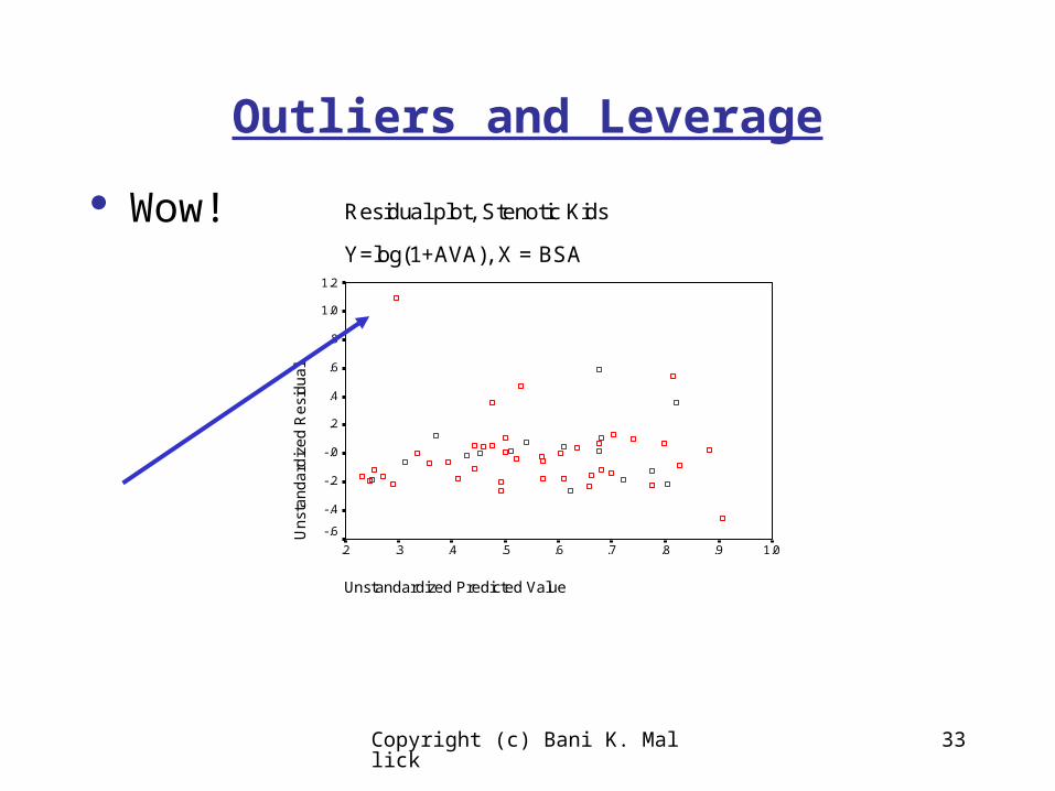
Outliers and Leverage
Wow! Residual plot, Stenotic Kids
Y=log(1+AVA), X = BSA
Unstandardized Predicted Value
1.0.9.8.7.6.5.4.3.2
Un
sta
nd
ard
ize
d R
esi
du
al
1.2
1.0
.8
.6
.4
.2
-.0
-.2
-.4
-.6
Copyright (c) Bani K. Mallick 34
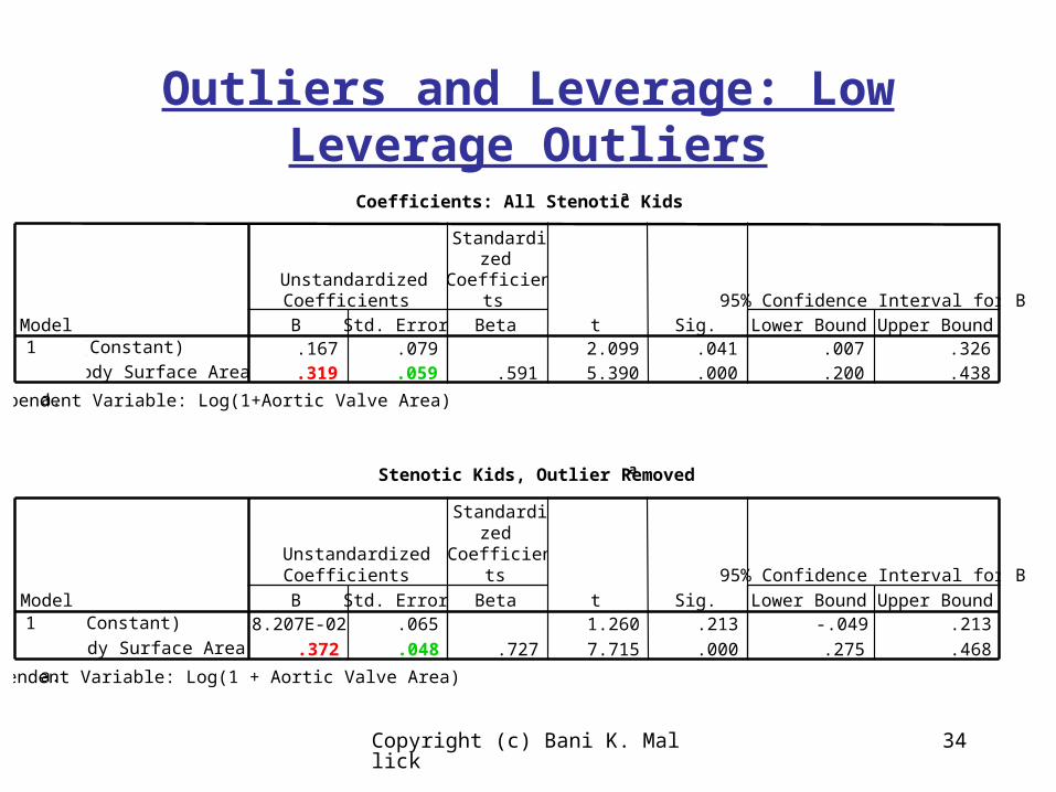
Outliers and Leverage: Low Leverage Outliers
Coefficients: All Stenotic Kidsa
.167 .079 2.099 .041 .007 .326
.319 .059 .591 5.390 .000 .200 .438
(Constant)
Body Surface Area
Model1
B Std. Error
UnstandardizedCoefficients
Beta
Standardized
Coefficients
t Sig. Lower Bound Upper Bound
95% Confidence Interval for B
Dependent Variable: Log(1+Aortic Valve Area)a.
Stenotic Kids, Outlier Removeda
8.207E-02 .065 1.260 .213 -.049 .213
.372 .048 .727 7.715 .000 .275 .468
(Constant)
Body Surface Area
Model1
B Std. Error
UnstandardizedCoefficients
Beta
Standardized
Coefficients
t Sig. Lower Bound Upper Bound
95% Confidence Interval for B
Dependent Variable: Log(1 + Aortic Valve Area)a.

Copyright (c) Bani K. Mallick 35
Remember: Outliers Inflate Variance!
ANOVA b
1.801 1 1.801 29.051 .000 a
3.348 54 6.200E-02
5.149 55
Regression
Residual
Total
Model1
Sum ofSquares df Mean Square F Sig.
Predictors: (Constant), Body Surface Areaa.
Dependent Variable: Log(1+Aortic Valve Area)b.
ANOVA b
2.352 1 2.352 59.526 .000 a
2.094 53 3.951E-02
4.446 54
Regression
Residual
Total
Model1
Sum ofSquares df Mean Square F Sig.
Predictors: (Constant), Body Surface Areaa.
Dependent Variable: Log(1 + Aortic Valve Area)b.
Copyright (c) Bani K. Mallick 36
Outliers and Leverage
The effect of a high leverage outlier is often to inflate your estimate of
With the outlier, the MSE (mean squared residual) = 0.0620
Without the outlier, the MSE (mean squared residual) is = 0.0395
So, a single outlier in 56 observations increases your estimate of by over 50%!
This becomes important later!
2
2
Copyright (c) Bani K. Mallick 37
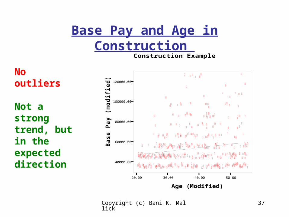
Base Pay and Age in Construction
20.00 30.00 40.00 50.00
Age (Modified)
40000.00
60000.00
80000.00
100000.00
120000.00
Bas
e P
ay (
mo
dif
ied
)
Construction Example
No outliers
Not a strong trend, but in the expected direction
Copyright (c) Bani K. Mallick 38
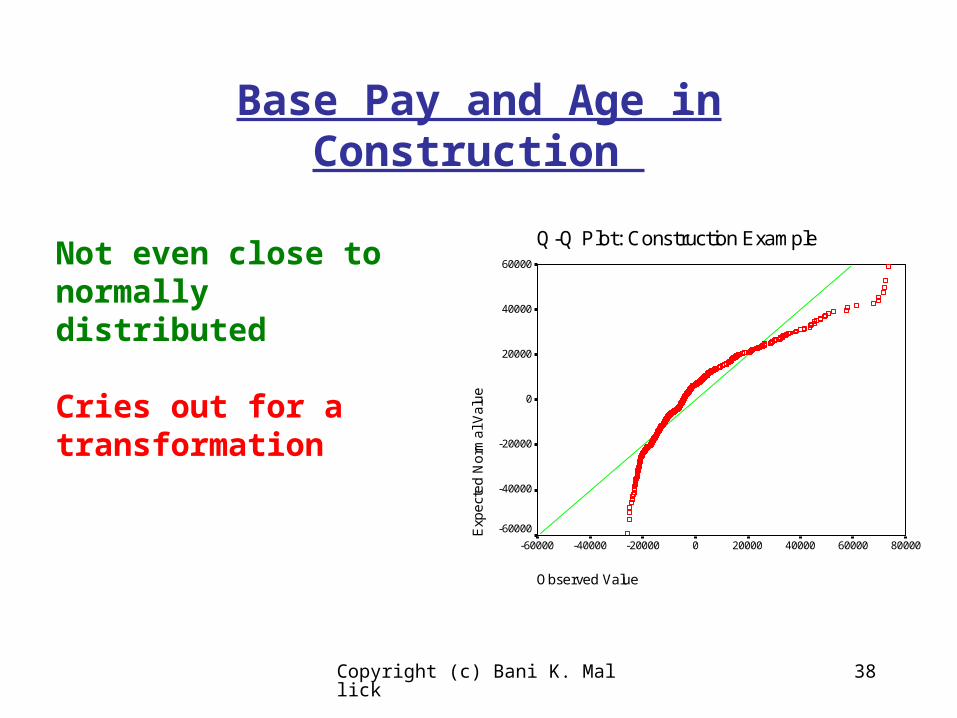
Base Pay and Age in Construction
Q-Q Plot: Construction Example
Observed Value
800006000040000200000-20000-40000-60000
Exp
ect
ed
No
rma
l Va
lue
60000
40000
20000
0
-20000
-40000
-60000
Not even close to normally distributed
Cries out for a transformation

Copyright (c) Bani K. Mallick 39
Log(Base Pay) and Age in Construction
20.00 30.00 40.00 50.00
Age (Modified)
8.00
9.00
10.00
11.00
Lo
g(B
ase
Pay
mo
dif
ied
- $
30,0
00)
Construction Example: Log ScaleExpected trend, but weak
Odd data structure: salaries were rounded in clumps of $5,000
Copyright (c) Bani K. Mallick 40
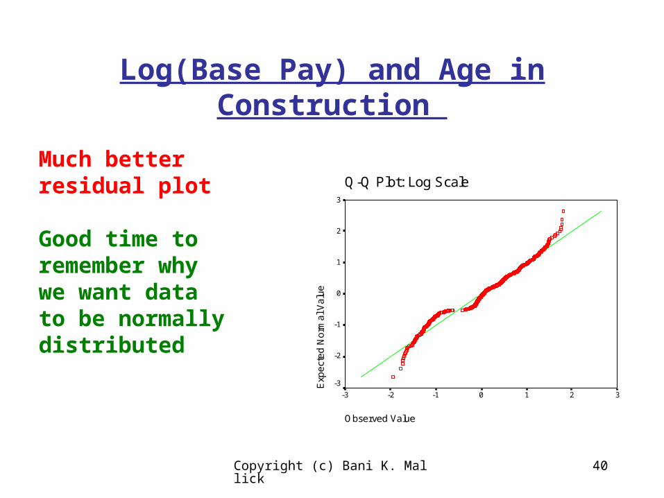
Log(Base Pay) and Age in Construction
Q-Q Plot: Log Scale
Observed Value
3210-1-2-3
Exp
ect
ed
No
rma
l Va
lue
3
2
1
0
-1
-2
-3
Much better residual plot
Good time to remember why we want data to be normally distributed

Copyright (c) Bani K. Mallick 41
Log(Base Pay) and Age in Construction
Log(Base Pay Modified - $30,000)
Sequence number
438
415
392
369
346
323
300
277
254
231
208
185
162
139
116
93
70
47
24
1
Co
ok'
s D
ista
nce
.02
.01
0.00
No real massive influential points, according to Cook’s distances
Copyright (c) Bani K. Mallick 42
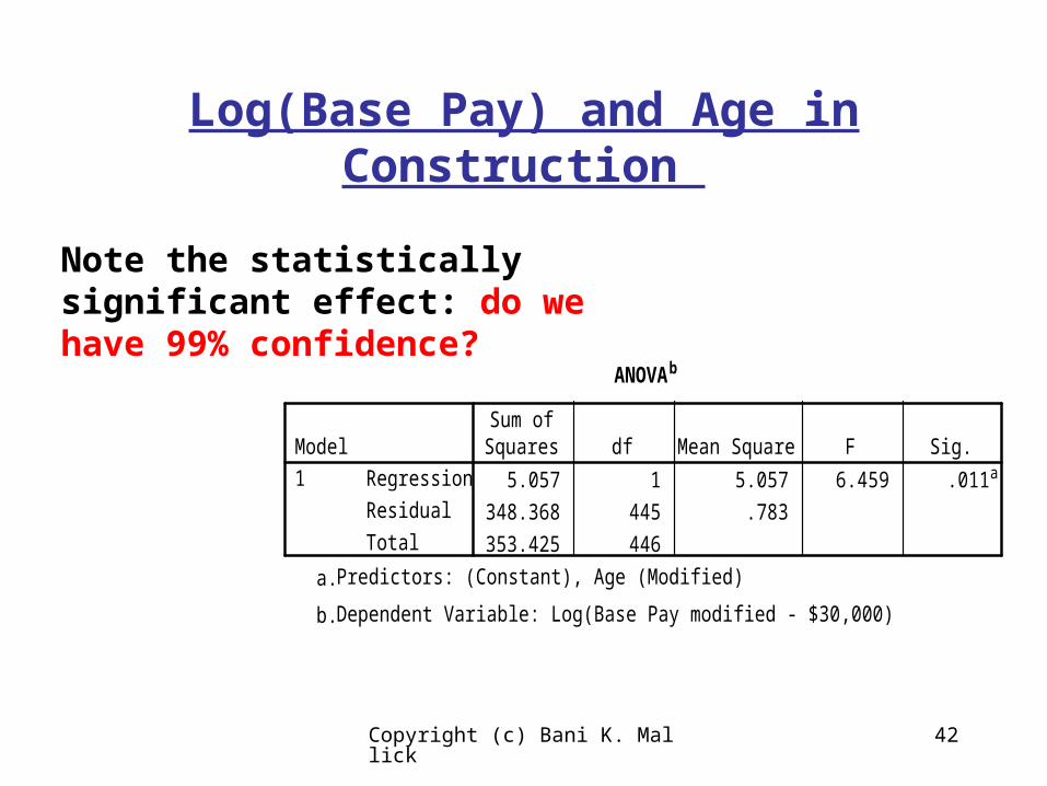
Log(Base Pay) and Age in Construction
ANOVAb
5.057 1 5.057 6.459 .011a
348.368 445 .783
353.425 446
Regression
Residual
Total
Model1
Sum ofSquares df Mean Square F Sig.
Predictors: (Constant), Age (Modified)a.
Dependent Variable: Log(Base Pay modified - $30,000)b.
Note the statistically significant effect: do we have 99% confidence?
Copyright (c) Bani K. Mallick 43
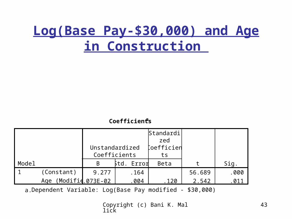
Log(Base Pay-$30,000) and Age in Construction
Coefficientsa
9.277 .164 56.689 .000
1.073E-02 .004 .120 2.542 .011
(Constant)
Age (Modified)
Model1
B Std. Error
UnstandardizedCoefficients
Beta
Standardized
Coefficients
t Sig.
Dependent Variable: Log(Base Pay modified - $30,000)a.