Copyright by Walter Benjamin Fair, Jr. 2019

Copyright

by

Walter Benjamin Fair, Jr.

2019

The Dissertation Committee for Walter Benjamin Fair, Jr. Certifies that this is the

approved version of the following dissertation:

An Integrated Model for Production of Marginal Oil Fields

Committee:

Tadeusz W. Patzek, Supervisor

Kamy Sepehrnoori, Co-Supervisor

Eric van Oort

Jon E. Olson

An Integrated Model for Optimizing Production of Marginal Oil Fields

by

Walter Benjamin Fair, Jr.

Dissertation

Presented to the Faculty of the Graduate School of

The University of Texas at Austin

in Partial Fulfillment

of the Requirements

for the Degree of

Doctor of Philosophy

The University of Texas at Austin

May 2019

Dedication

I dedicate this work to my late parents, Walter B. Fair, Sr. and Marianne Fair, who provided

a loving home while they instilled within me a love for learning and a work ethic; to my

maternal grandfather, Hans A. Harrfeldt, who always encouraged me to study; to my wife

Argentina Fair, who supported me throughout my studies; and to my children, step-children

and grandchildren, who always offered words of encouragement and overlooked the fact

that going back to school was simply a crazy thing to do for an old man.

v

Acknowledgements

No work can be done in isolation and this dissertation is no exception. I have

certainly gained insight from many people throughout my life and it would be impossible

to name all of them. I would like to express special thanks to my supervisors, Dr. Patzek

and Dr. Sepehrnoori, for putting up with me and keeping me focused on the tasks at hand.

As well, many discussions with Dr. M. Shirdel were very useful in trying to model transient

pipe flow. Thanks also to Ample Resources, Inc. for permission to use field data to validate

the work documented herein.

vi

An Integrated Model for Optimizing Production of Marginal Oil Fields

Walter Benjamin Fair, Jr., Ph.D.

The University of Texas at Austin, 2019

Co-Supervisors: Tadeusz W. Patzek and Kamy Sepehrnoori

For the optimization of production in an operating marginal oil field, it is necessary

to consider the reservoir inflow, the artificial lift systems, as well as the surface facilities.

Since most reservoir simulation software does not include detailed facility modeling, an

integrated model of an entire field has been developed including the surface facilities, to

allow detailed modeling of the entire field operation. This model is useful for optimizing

production and for use in field surveillance activities, as well as investigating the

applicability of simplified engineering assumptions.

vii

Table of Contents

Chapter 1: Introduction ...........................................................................................1

Organization ....................................................................................................3

Chapter 2: Oil Field Flow Network ........................................................................5

Generic Field Description ...............................................................................6

Design Goals ...................................................................................................7

Description of Flow Network .........................................................................7

Implementation .............................................................................................10

Flow Network ......................................................................................13

Name: ..........................................................................................13

Parameters: ..................................................................................13

Methods.......................................................................................13

Flow Equipment ...................................................................................14

Name: ..........................................................................................14

Parameters: ..................................................................................14

Methods.......................................................................................14

Flow Stream .........................................................................................15

Name: ..........................................................................................15

Parameters: ..................................................................................15

Methods.......................................................................................15

Chapter 3: Multiphase Pipe Flow .........................................................................17

Flow Equations .............................................................................................18

Conservation of Mass .................................................................19

Liquid Momentum ......................................................................19

Gas Momentum ...........................................................................19

Oil + Water Mass Balance ..........................................................20

Water Mass Balance ...................................................................20

Total Energy................................................................................20

Annular Flow ..............................................................................20

viii

Flow Patterns ..............................................................................21

Fluid Drag ...................................................................................22

Interfacial Drag ...........................................................................22

Initial and Boundary Conditions .................................................23

Solution of Flow Equations ..........................................................................23

Momentum Balance Equations ............................................................24

Mass Balance Equations ......................................................................25

Energy Balance Equation .....................................................................26

Validation ......................................................................................................27

Chapter 4: Multiphase Separators .........................................................................35

Vertical Separator .........................................................................................36

Fundamental Equations ........................................................................36

Numerical Solution ..............................................................................39

Chapter 5: Well Model..........................................................................................42

Constant Rate Well .......................................................................................42

Beam Pumps .................................................................................................43

Rod Motion ..........................................................................................45

Surface Pumping Unit ..........................................................................48

Downhole Pump...................................................................................49

Casing Annulus .............................................................................................50

Reservoir and completion model ..................................................................51

Chapter 6: Auxiliary Flow Equipment ..................................................................54

Flow Junctions ..............................................................................................54

Tanks .............................................................................................................55

Surface Pumps ..............................................................................................55

Compressors ..................................................................................................55

Chokes...........................................................................................................56

ix

Chapter 7: Field Applications ...............................................................................57

Conclusions and Recommendations ......................................................................62

Conclusions: ..................................................................................................62

Recommendations: ........................................................................................62

Appendices .............................................................................................................65

Appendix A1: Fluid Properties ....................................................................65

Black Oil PVT Model ...................................................................................65

Brine ..............................................................................................................67

Composition .........................................................................................67

Density .................................................................................................67

Formation Volume Factor ....................................................................68

Viscosity ..............................................................................................68

Oil ..............................................................................................................69

Density .................................................................................................69


Solution Gas-Oil Ratio .........................................................................70

Viscosity ..............................................................................................70

Heat Capacity .......................................................................................71

Gas ..............................................................................................................71

Z Factor ................................................................................................72

Density .................................................................................................72


Viscosity ..............................................................................................73

Heat Capacity .......................................................................................73

Appendix A2: Parameter Estimation ...........................................................74

Heat Transfer Coefficients ............................................................................74

References ..............................................................................................................77

1

Chapter 1: Introduction

In order to optimize production from marginal oil fields, it is necessary to consider

reservoir, well, and surface facility performance. The purpose of this research is to develop

a complete model for use in evaluating efficient methods for operating oil fields including

marginal fields.

According to the US Department of Energy, stripper wells are defined as wells

producing less than 10 barrels of oil per day. The Interstate Oil and Gas Compact

Commission IOGCC (2008) reports that in 2008 there were over 396,000 stripper wells in

the US producing over 291,000,000 bbl of oil and over 130,000 stripper wells producing

120,000,000 bbl of oil were in Texas. Other sources indicate that as much as 1 out of every

6 barrels of oil in the US is produced from stripper wells. In 2009, the Independent

Petroleum Association of America estimated that 85% of US wells produce less than 15

bbl of oil per day and account for about 20% of the total US production. Since producing

wells naturally exhibit declining production rates, more wells will inevitably be added to

these numbers each year. Because of the low producing rates, most of these wells are

marginally economic and since most are not operated by major companies with research

facilities, there is little fundamental corporate research directly supporting development

and operation of these wells. On account of the strategic importance of marginal wells and

the lack of industry research, the study of these wells will be an important contribution to

the energy outlook for the State of Texas and the US.

Optimizing production from such marginal wells is a daunting effort for reasons

documented in the IOGCC (2008) report. In order to optimize production and ultimate

recovery from an oil field, it is necessary to consider reservoir fluid flow, recovery

processes, well design, artificial lift, surface facilities, operational constraints and logistical

2

problems. With the availability of cheap computing and communication facilities, there

has been an emphasis on real-time monitoring and control where in other industries

concepts such as data mining and real time analysis have been applied to great advantages.

While much work has been done on each of the individual parts of this overall problem,

the full integration of the parts has not generally been done, especially on a scale suitable

for application to marginally economic wells and fields. In particular, it appears that most

of the work toward real-time monitoring and surveillance applies mainly to larger,

economically viable fields, but cannot obviously be applied to the vast majority of marginal

fields and wells due to infrastructure and economic considerations. The result of this

research is the development of an integrated model for use in evaluating efficient methods

for operating all types of oil fields including marginal fields.

Besides the problem of integrating reservoirs, wells, surface facilities, operational

and logistical systems, the relative time scale at which each subsystem operates adds

additional complexity. Normally, reservoir processes may take weeks, months or years to

reach steady-state conditions, while the flow in wells may stabilize in a period of hours or

days. The use of beam pumps may force cycles of hours with the use of timers and pump-

off controllers, while pulsating flow due to individual pump strokes can be measured in

seconds. In the surface facilities, compressors and pumps respond to changes in seconds,

while separators usually have residence time on the order of minutes. Since it is generally

impractical to run a typical reservoir simulator with time steps on the order of minutes,

seconds or less, a realistic means of scaling the time behavior of the various systems is

important. It is not clear that simple time averaging of models can properly represent

phenomena occurring at smaller time scales that may have an important effect on

operations and economics.

3

Aside from the model integration challenges mentioned, the problem of optimizing

production from marginal wells is a particularly complex endeavor. Low producing rates

can be caused by poor reservoir quality, high fluid viscosity, low pressure, high water

saturation, sand production, mechanical problems, artificial lift constraints, and other

considerations. In addition, although technical solutions to the problems may be known,

low rates correspond generally to low revenue that may easily make the implementation

uneconomic. Furthermore, since these wells are comparatively low income producers,

resources are often not spent on data acquisition. As a result, the application of technology

and the acquisition of data must be based upon adding value in the presence of tight

constraints on economics, expenditures and data availability.

ORGANIZATION

Since the purpose of this work is to develop an integrated model, inevitably the

subjects involved will be intertwined; hence, no simple linear organization is possible.

Chapter 2 presents the field network model that integrates all of the individual parts of a

full field model developed in this work. The following Chapters 3, 4, and 5 present detailed

models of the pipes, separators and wells that are incorporated into the integrated model,

each of which presents complex modeling challenges. Chapter 6 presents a summary of

auxiliary equipment models that were not modeled in detail, such as flow junctions, pumps,

compressors, and tanks. Finally, Chapter 7 presents examples of the use of the model. Since

fluid properties and other parameters are important in the application of the integrated

model, the appendices document the fluid properties and parameters, as well as methods

for estimation when data are not available.

As a result of this work, an integrated field modeling framework has been produced

and implemented. The resulting software named Integrated Field Model (IFM) has been

4

written in C# using Microsoft Visual Studio™ that can be run on many Windows™

operating systems. The software has been tested on Windows Vista, Windows 7 and

Windows 8 and Windows 10.

The purpose of this research is to develop a complete model for use in evaluating

efficient methods for operating all types of oil fields including marginal fields

5

Chapter 2: Oil Field Flow Network

In order to represent flow in an entire field consisting of reservoirs, wells, pipes,

separators, pumps, compressors, tanks, and other assorted equipment, it is necessary to

develop a framework for representing the flow network and determine computational

methods to solve the coupled flow equations for each entity, as well as the network as a

whole. This chapter summarizes the definition of a flow network that will serve as the

framework for flow calculations in the integrated field model.

To have a basis for the design and implementation of the integrated field model and

to ensure that it can be applied to actual marginal fields, a generic marginal field is first

defined. The defined generic field should have enough flexibility to allow representation

of the majority of actual marginal fields. In order to model, history match and optimize

total recovery from marginal fields, a computational framework is needed that can

represent the necessary equipment and fluid flow within the wells and through the surface

equipment. In order to optimize the recovery, production and operations, the framework

should be capable of multiphase fluid flow calculations, allow the estimation of operating

costs and be amenable to data input and output requirements. Within the overall integrated

system, numerical models of each of the defined subsystems can then be developed. These

will vary in complexity depending upon the detail required within the overall system

model. Some modules will require detailed, finite difference representations (i.e. flowlines,

separators, and reservoirs), while other modules may be simply represented by a pressure

change, perhaps with computed horsepower requirements (i.e. pumps, chokes,

compressors, etc.).

6

GENERIC FIELD DESCRIPTION

According to information provided in, as well as personal experience, a typical

marginal oil field in the US consists of low-rate oil wells often with large amounts of

water producing by beam pump. Flow lines connect the wells to a header where they flow

into a series of separators. Gas may be produced from the casing head of the wells and

taken off the separators and may be compressed for sale or field use, or in few cases be

flared. In some fields, casing gas is produced through a separate compression system to

reduce the bottomhole pump intake pressure and increase reservoir inflow into the

wellbore. Free water is usually taken off from each separator stage and stored in a tank for

trucking or be injected into a disposal well. Oil taken from the separators may require

additional separation to yield acceptable quality oil for sale. Finally, the oil is held in a

stock tank at atmospheric pressure and ambient temperature where it awaits sales by either

a LACT unit or transportation by truck. As a result, without much loss of generality, a flow

system consisting of reservoirs and wells, flowlines, various stages of separators and tanks

is chosen as a typical marginal field model. A sketch of such a field flow diagram is shown

in Figure 2.1. Additional reservoirs, wells, separators, pumps, compressors and chokes can

be included as required in order to represent actual field operations.

The basic flow system can be represented by a network flow diagrams, which is

assumed to have no cyclic paths, thus simplifying the computational procedures. If we

assume that suitable check valves are installed at strategic locations (as is common to

prevent backflow), this system can be represented mathematically as a directed acyclic

graph, often referred to as a digraph or DAG. A mathematical abstraction of an acyclic

digraph is shown in Figure 2.2. By using a mathematical abstraction to represent the flow

system, many techniques from computer science (Aho et al., 1983) can be applied to

represent and manipulate the network flow model.

7

DESIGN GOALS

To design a workable integration framework, it is useful to list the requirements a

workable model would have. These requirements then serve as a guide in considering

options and as a check on the feasibility of the final defined model. The design goals for

the flow system model are as follows:

1. The model must be capable of representing the applicable physics of fluid

flow within a typical oil field.

2. The model must be represented in a computationally efficient manner for

solution on typical desktop and laptop computers.

3. The model must be extensible, so that additional equipment can be added at

a later date and not be limited to flow equipment currently envisioned.

4. The model must be capable of representing arbitrary connections between

equipment items so that a wide variety of configurations can be represented.

5. An algorithm based on physical considerations must be developed for

solution of the overall flow network.

6. The system must provide a general means for detailed models, internal to

each specific flow equipment items, to be developed.

DESCRIPTION OF FLOW NETWORK

The defined flow system used in this work is based on an abstract directed acyclic

graph (Aho, 1983) where each equipment item is represented by a node and where arcs

represent the flow streams or connections between equipment. This is a standard approach

previously described by various authors to represent flow networks (cf. Daugherty and

Franzini, 1965); Himmelblau and Bischoff, 1968). Using an object-oriented design

philosophy, equipment objects (nodes) are those items with volume and whose state

8

changes occur internally, while flow streams (arcs) have no volume and serve mainly as

pressure measurement points and connections between items.

For each equipment object within the network, the conservation of mass, the

conservation of linear momentum and the conservation of energy can be applied to

represent fluid flow and mass storage within the equipment that the node represented.

Examples are pipes, wells, separators, tanks, etc.

Flow streams, however, have no volume and represent the connections between

equipment nodes. It is assumed that streams have properties of mass flow rates, temperature

and pressure, but no internal mass is stored within a flow stream. The continuity of flowing

properties through the flow streams is assumed.

The overall network is represented computationally as an object containing a list of

flow equipment items and a list of flow streams. Each equipment item is identified by an

equipment type and a name, while flow streams are only identified by the equipment items

that they connect.

The fundamental equations describing flow in the network (cf. Daugherty, 1965)

consist of mass, momentum, and energy balance relations for each subpart of the network

and continuity relationships. Since we will implement the network using detailed physical

models for each equipment node, all of the balances will automatically be satisfied over

every part of the network, as well as the network as a whole. In addition, a continuity

constraint is needed, which is automatically satisfied by detailed internal modeling in each

node and the constraint that each stream (i.e. connection between nodes) can have only a

single temperature, pressure, and flow rate at any time. In other words, the outlet conditions

from one equipment item must be the same as the inlet conditions for the following item.

As will be seen, due to the implementation, this will be automatically ensured in the flow

network model.

9

In order to solve the fundamental flow equations in the flow network, an iterative

multi-pass algorithm has been devised. While considering flow especially through

junctions where mass conservation requires a balance between the flow rates, pressures

and temperatures of individual complex flow equipment items, it is apparent that the

simultaneous solution of the equations of momentum, mass, and energy throughout a

complex network would be difficult and likely impractical to implement. As a result, an

iterated sequential solution algorithm has been devised and the following solution

procedure has been implemented.

1. Sort the network equipment items in order from sources to sinks using the

following procedure:

a. Create an empty list of equipment items, then search through the

network equipment and add all equipment items that do not have a

defined inlet.

b. For each equipment item in the list

i. For each outlet stream, find the equipment associated with

the outlet and add it to the list.

2. Set simulation time to zero and initialize the flow system using the

following procedure:

a. Beginning at the sources, traverse the flow network and set all rates

to zero and all temperatures to a specified ambient temperature with

appropriate fluid contents.

b. Beginning at the sinks, traverse the network in a reverse direction

and compute the inlet pressure for each equipment item considering

static equilibrium within each equipment item.

10

3. Iterate through the network flow calculations until the flow rates,

temperature and pressure of all flow streams do not change within a

specified tolerance using the following procedure:

a. Beginning at the sources, traverse the flow network in a forward

direction and solve the applicable flow equations to determine the

outlet flow rates for each equipment item in order, assuming the

pressure, temperature and inlet flow rates are known.

b. Beginning at the sinks, traverse the flow network in a reverse

direction to compute the pressure at the inlet of each flow equipment

item assuming that the flow rates, temperature and outlet pressures

are known.

c. Beginning at the sources, traverse the network once again in a

forward direction and compute the outlet temperature for each

equipment item assuming the flow rates, pressures and inlet

temperature are known.

4. Print or save necessary information, advance the time step and return to step

3.

IMPLEMENTATION

The entire integrated flow model was implemented in the C# programming

language using Microsoft Visual StudioTM 2008. In order to enforce the flow calculations,

certain parameters and methods are required for all flow equipment and flow streams.

These are implemented in the object inheritance hierarchy and the use of override and

virtual methods in the C# programming language. The overall network programming

11

objects are defined as follows: It should be noted however, that each equipment item will

add additional detail to that specified here.

In order to provide input data to IFM, an XML file format was selected because it

is plain text and easily created and has enough descriptors to make it readable even to

persons not trained in the use of the software. Following is a representative data file with a

detailed description.

1. <?xml version="1.0" encoding="utf-8"?> 2. <IFM> 3. <Project Name="2 Beam Pump Wells to Tank"> 4. <Environment Temperature="60" /> 5. </Project> 6. <FluidSystem Type="BlackOil"> 7. <Component Name="GAS" Type="Gas" GasGravity="0.7" /> 8. <Component Name="OIL" Type="Oil" APIGravity="30" /> 9. <Component Name="WTR" Type="Water" Salinity="0" /> 10. <Phase Name="AQUEOUS" Type="Aqueous" /> 11. <Phase Name="HCLIQ" Type="HCLiquid" /> 12. <Phase Name="HCVAP" Type="HCVapor" /> 13. </FluidSystem> 14. <Network> 15. <Equipment Type="Well" Name="W1" X="0" Y="4000" Elevation="0"> 16. <Tubing ID="0.166666666666667" OD="0.19375" Roughness="0.0075"

Length="4000" Anchor="True" /> 17. <Casing ID="0.416666666666667" OD="0.4583333333333" Roughness="0.00075"

Length="4000" Closed="False" Vent="14.7" /> 18. <Completion Type="Radial" k="10.0" h="10.0" phi="0.1" S="0.0" T="110.0"

pi="100.0" rw="0.3" re="1000.0" NR="10" WaterCut="0.0" GOR="3.0" /> 19. <LiftMode Type="RodPump">

a. <SurfaceUnit A="30.0" C="111.07" I="48.0" P="132.0" H="213.99" G="45.13" R="42.0" />

b. <Rods Type="Steel" Length="4000.0" Diameter="0.75" Segments="20" />

c. <Pump Diameter="1.5" Efficiency="1.0" InitialHt="4.0" /> d. <Operation SPM="6.0" Ttbg="60.0" />

20. </LiftMode> 21. </Equipment> 22. <Equipment Type="Well" Name="W2" X="3000" Y="-2000" Elevation="0"> 23. <Tubing ID="0.166666666666667" OD="0.19375" Roughness="0.0075"

Length="3000" Anchor="True" /> 24. <Casing ID="0.416666666666667" OD="0.4583333333333" Roughness="0.00075"

Length="3000" Closed="False" Vent="14.7" />

12

25. <Completion Type="Radial" k="10.0" h="10.0" phi="0.1" S="0.0" T="110.0" pi="100.0" rw="0.3" re="1000.0" NR="10" WaterCut="0.0" GOR="3.0" />

26. <LiftMode Type="RodPump"> a. <SurfaceUnit A="30.0" C="111.07" I="48.0" P="132.0" H="213.99"

G="45.13" R="42.0" /> b. <Rods Type="Steel" Length="3000.0" Diameter="0.75" Segments="20"

/> c. <Pump Diameter="1.5" Efficiency="1.0" InitialHt="4.0" /> d. <Operation SPM="5.0" Ttbg="60.0" />

27. </LiftMode> 28. </Equipment> 29. <Equipment Type="Pipe" Name="P1" X="0" Y="4000" Elevation="0"> 30. <End X="10000" Y="0" Elevation="0" /> 31. <Dimensions ID="0.166666666666667" OD="0.19375" Roughness="6E-05"

Length="10770.00" /> 32. <Model Segments="54" /> 33. </Equipment> 34. <Equipment Type="Pipe" Name="P2" X="3000" Y="-2000" Elevation="0"> 35. <End X="10000" Y="0" Elevation="0" /> 36. <Dimensions ID="0.166666666666667" OD="0.19375" Roughness="6E-05"

Length="7280" /> 37. <Model Segments="36" /> 38. </Equipment> 39. <Equipment Type="Junction" Name="J1" X="0" Y="4000" Elevation="0" /> 40. <Equipment Type="Junction" Name="J2" X="3000" Y="-2000" Elevation="0" /> 41. <Equipment Type="Junction" Name="J3" X="10000" Y="0" Elevation="0" /> 42. <Equipment Type="Pipe" Name="P3" X="10000" Y="0" Elevation="0"> 43. <End X="16000" Y="0" Elevation="0" /> 44. <Dimensions ID="0.166666666666667" OD="0.19375" Roughness="6E-05"

Length="6000" /> 45. <Model Segments="30" /> 46. </Equipment> 47. <Equipment Type="Tank" Name="T1" X="16000" Y="0" Elevation="0"> 48. <Dimensions Height="20" Diameter="8" Inlet="1" PrimaryPhase="HCLIQ" /> 49. <Operation Pressure="100.0" Temperature="60" /> 50. </Equipment> 51. <Stream FromEq="W1" FromName="TUBING" ToEq="J1" ToName="I1"

BackFlow="TRUE" /> 52. <Stream FromEq="W1" FromName="CASING" ToEq="J1" ToName="I2"

BackFlow="True" /> 53. <Stream FromEq="J1" FromName="O1" ToEq="P1" ToName="INLET"

BackFlow="TRUE"/> 54. <Stream FromEq="P1" FromName="OUTLET" ToEq="J3" ToName="I1"

BackFlow="TRUE"/> 55. <Stream FromEq="W2" FromName="TUBING" ToEq="J2" ToName="I1"

BackFlow="TRUE" /> 56. <Stream FromEq="W2" FromName="CASING" ToEq="J2" ToName="I2"

BackFlow="True" /> 57. <Stream FromEq="J2" FromName="O1" ToEq="P2" ToName="INLET"

BackFlow="TRUE"/>

13

58. <Stream FromEq="P2" FromName="OUTLET" ToEq="J3" ToName="I2" BackFlow="TRUE"/>

59. <Stream FromEq="J3" FromName="O1" ToEq="P3" ToName="INLET" BackFlow="TRUE"/>

60. <Stream FromEq="P3" FromName="OUTLET" ToEq="T1" ToName="INLET" BackFlow="TRUE" />

61. </Network> 62. <Initialize> 63. <Equipment Name="P1" Pout="True" Pin="False" Qo="0" Qw="0" Qg="0"

HL="1.0" FW="0.0" RS="2.0" /> 64. <Equipment Name="P2" Pout="True" Pin="False" Qo="0" Qw="0" Qg="0"

HL="1.0" FW="0.0" RS="2.0" /> 65. <Equipment Name="P3" Pout="True" Pin="False" Qo="0" Qw="0" Qg="0"

HL="1.0" FW="0.0" RS="2.0" /> 66. </Initialize> 67. <SurfaceUnit1 A="56.0" C="48.17" I="48.0" P="57.50" H="106.63"

G="45.13" R="10.0" Stroke="24" /> 68. <SurfaceUnit2 A="30.0" C="111.07" I="48.0" P="132.0" H="213.99"

G="45.13" R="42.0" Stroke="24" /> 69. <SurfaceUnit3 A="129.0" C="111.07" I="111.0" P="132.0" H="232.0" G="96"

R="42.0" Stroke="100"/> 70. <SurfaceUnit4 A="64.0" C="64.0" I="64.0" P="74.5" H="126.13" G="51.13"

R="24.0" Stroke="48"/> 71. <SurfaceUnit5 A="64.0" C="64.0" I="64.0" P="74.5" H="126.13" G="51.13"

R="16.0" Stroke="32"/> 72. </IFM>

Flow Network

Name:

FlowNetwork

Parameters:

Fluids – the fluid system properties to be used in the flow calculations

Equipment – a sorted list of Flow Equipment items contained in the network

Streams – a list of Flow Stream items contained in the network

Methods

None

14

Flow Equipment

Name:

FlowEquipment

Parameters:

Name– the name of the equipment item

EquipmentType– the type of equipment, i.e. Separator, Pipe, Well, etc.

Location– the x- and y-coordinates and elevation where the item is located

Inlets– a list of Flow Stream items representing flow inlets to the equipment item

Outlets– list of Flow Stream items representing flow outlets from the equipment

item

Methods

Initialize – set the initial conditions for the equipment item

SaveState – save the state of the equipment item prior to a time step, must be

implemented by each equipment type

GetOutletRates – solve flow equations internal to the equipment to determine

the outlet flow rates; must be implemented by each equipment type

GetInletPressures – solve flow equations internal to the equipment to

determine the outlet pressures; must be implemented by each equipment

type

GetOutletTemperatures – solve flow equations internal to the equipment to

determine the outlet temperatures; must be implemented by each equipment

type

15

Flow Stream

Name:

FlowStream

Parameters:

FromName – the name of the FlowEquipment where the stream originates

FromEquip – the FlowEquipment where the stream originates

ToName – the name of the FlowEquipment where the stream ends

ToEquip – the FlowEquipment where the stream ends

CanBackFlow – indicates whether fluids can flow in reverse through the stream

CurrentState – the current state of flow rates, temperature and pressure for the

stream

SavedState – the state of flow rates, temperature and pressure for the stream at

the last time step

LastState – the state of flow rates, temperature and pressure for the stream at

the last iteration

Methods

Connect – link the inlet and outlet equipment to the stream

SaveState – save the flow rates, temperature and pressure at the start of a time

step

SaveIterationState – save the flow rates, temperature and pressure at the start

of an iteration.

16

Figure 2.1. Simplified flow diagram of a typical marginal oil field.

Figure 2.2. Example of a Directed Acyclic Graph (DAG, from Wikipedia).

SWD

Oil Sales

Gas Sales

Oil Tank

Water Tank

Sep 1

Sep 2

Res 1

Res 2

W 1

W 2 W 3

17

Chapter 3: Multiphase Pipe Flow

Within the well and surface facilities, a large portion of the fluid flow occurs within

pipes and piping networks. In various parts of the well and facilities, fluids may be single-

phase, two-phase or three-phase; so it is necessary to develop methods to model all three

situations. In addition, since a significant part of this work depends on modeling unsteady

state flow, the typical assumptions of steady-state, time-invariant flow cannot necessarily

be invoked. An overview of multiphase flow modeling in wellbores is presented in Brill

and Mukherjee (Brill and Mukherjee, 1999) and a detailed treatment of more general

multiphase flow is contained in Kolev (Kolev, 2002), (Govier and Aziz, 2008) and Shoham

(Shoham, 2006).

Single-phase fluid flow has been studied extensively and finds wide application in

many industries. In general, the flow is analyzed using the conservation of mass and the

conservation of linear momentum as well as the conservation of energy when thermal

effects are important. It is generally necessary to incorporate an empirical friction factor to

account for variations in flow velocity within a pipe as well as accounting for the presence

of a boundary layer in turbulent flow (Bird et al., 2007).

For multiphase, multicomponent flow, the evaluation is more complex since

equations for the conservation of mass and the conservation of linear momentum of each

component are required, as well as the conservation of total energy. In addition, since phase

changes and interphase mass transfer may occur along the flow path, a flash procedure is

needed to describe the fluid compositions at each point and an equation-of-state is required

to determine the corresponding phase properties, where thermodynamic equilibrium is

assumed locally.

18

FLOW EQUATIONS

For multiphase, multicomponent flow, a mass conservation and a momentum

conservation equation are written for infinitesimal pipe segments for each component with

an overall conservation of energy relation to account for thermal effects. The derivation is

not presented here, but a detailed derivation is given in Shirdel (Shirdel, 2010) and in

RELAP5 (RELAP5, 2012). An analysis of two-phase flow in inclined pipes was presented

by Beggs and Brill (Brill and Mukherjee, 1999) for steady-state flow; however in this

present work multiphase transient flow was represented following the techniques presented

in the RELAP5 documentation (RELAP5, 2012) as in (RELAP5, 2012) and Shirdel

(Shirdel, 2013). The fundamental equations are summarized as follows, where a black oil

compositional model is assumed.

As was done by Shirdel (Shirdel, 2010), the momentum balances were taken by

phase, rather than by component. Although this ignores the effect of interphase momentum

transfer due to changes in the solution gas in a black oil model, the effect is small, and it

was assumed that all the gas momentum is in the vapor phase. Due to the generally low

mass of solution gas compared to oil, this assumption appears to be warranted. Note also

that the momentum equations were simplified by expanding the terms containing velocity

and substituting the mass balance equations as was done in RELAP5 (RELAP5, 2012) and

Shirdel (Shirdel, 2013). Note that the momentum equations contain terms that describe

drag effects for contact between the fluid and pipe wall and pipe annulus, FwL, FaL, FwG and

FaG, as well as a term to describe the drag between the liquid and the gas phases, FLG. These

terms must be determined from multiphase flow correlations and will be described in a

following section.

In modeling fluid flow in rod pumped wells, the fluid flows in the annulus between

the tubing and the rods. In that case, there is drag along both the inside and the outside

19

diameters and additionally the inside pipe wall will likely be in motion. Calculation of the

fluid drag for rods and couplings is covered in Chapter 5.

Conservation of Mass

𝜕

𝜕𝑡(𝐻𝐿𝜌𝐿 + 𝐻𝐺𝜌𝐺) +

𝜕

𝜕𝑥(𝐻𝐿𝜌𝐿𝑣𝐿 + 𝐻𝐺𝜌𝐺𝑣𝐺) = 0 ........................................... (3.1)

Liquid Momentum

𝐻𝐿𝜌𝐿𝜕𝑣𝐿

𝜕𝑡+

1

2𝐻𝐿𝜌𝐿

𝜕𝑣𝐿2

𝜕𝑥 + 144𝑔𝑐

𝜕

𝜕𝑥(𝐻𝐿𝑝) + 𝐻𝐿𝜌𝐿𝑔 𝑠𝑖𝑛𝜃 + 𝐹𝑤𝐿 + 𝐹𝑎𝐿 − 𝐹𝐿𝐺 = 0 ............. (3.2)

Gas Momentum

𝐻𝐺𝜌𝐺𝜕𝑣𝐺

𝜕𝑡+

1

2𝐻𝐺𝜌𝐺

𝜕𝑣𝐺2

𝜕𝑥 + 144𝑔𝑐

𝜕

𝜕𝑥(𝐻𝐺𝑝) + 𝐻𝐺𝜌𝐺𝑔 𝑠𝑖𝑛𝜃 + 𝐹𝑤𝐺 + 𝐹𝑎𝐺 + 𝐹𝐿𝐺 = 0 .......... (3.3)

Where HL = liquid holdup (i.e. volume fraction of liquid, fraction)

HG = gas holdup (i.e. volume fraction of gas)

L = liquid (oil + water) density (lb/ft3)

G = gas phase density (lb/ft3)

gc = gravitational constant (32.17 ft/sec2)

= angle of flow above the horizontal in Rad

p = pressure (psia)

For each component, the mass balance for that component is the sum of

contributions across all phases. For computational purposes, mass balance equations for

oil, gas and water components, as well as oil plus gas, water plus oil, water plus gas, and

total oil, water, and gas mixtures are interchangeable and any 3 of the relationships can be

selected. Since the pressure calculation is mostly dependent on the total mass balance and

the formulation uses total liquid (oil plus water) in the momentum relations, the equations

chosen here are 1) total mass balance (oil plus water plus gas), the liquid mass balance (oil

plus water) and the water mass balance. It is also assumed that the pressure and the

20

temperature in all phases are equal at any point along the pipe length and do not vary across

the pipe diameter. The equations are:

Oil + Water Mass Balance

𝜕

𝜕𝑡{𝐻𝐿 [𝑓𝑊𝜌𝑊 + 𝑓𝑂 (𝜌𝑂 −

𝑅𝑠�̂�𝐺

5.6146)]} +

𝜕

𝜕𝑥{𝐻𝐿 [𝑓𝑊𝜌𝑊 + 𝑓𝑂 (𝜌𝑂 −

𝑅𝑠�̂�𝐺

5.6146)] 𝑣𝐿} = 0 ............... (3.4)

Water Mass Balance

𝜕

𝜕𝑡(𝐻𝐿𝑓𝑊𝜌𝐿) +

𝜕

𝜕𝑥(𝐻𝐿𝑓𝑊𝜌𝐿𝑣𝐿) = 0 .................................................................. (3.5)

Total Energy

𝜕

𝜕𝑡[𝐻𝐿𝜌𝐿 (ℎ𝐿 +

𝑣𝐿2

2𝑔𝑐𝐽𝑐−

144 𝑝

𝐽𝑐𝜌𝐿) + 𝐻𝐺𝜌𝐺 (ℎ𝐺 +

𝑣𝐺2


144 𝑝

𝐽𝑐𝜌𝐺)] + (𝐻𝐿𝜌𝐿𝑣𝐿 + 𝐻𝐺𝜌𝐺𝑣𝐺)𝑔 𝑠𝑖𝑛𝜃 +

𝜕

𝜕𝑥[𝐻𝐿𝜌𝐿 (ℎ𝐿 +

𝑣𝐿2

2𝑔𝑐𝐽𝑐) 𝑣𝐿 + 𝐻𝐺𝜌𝐺 (ℎ𝐺 +

𝑣𝐺2

2𝑔𝑐𝐽𝑐) 𝑣𝐺] + 𝑈𝑆(𝑇 − 𝑇𝑒𝑥𝑡) = 0 .......................... (3.6)

The energy balance is taken over all phases and incorporates an overall heat loss

coefficient, U, that acts across the internal pipe perimeter, S, to describe heat lost from the

fluids. Again, it is assumed that all phases, as well as the pipe material, are at the same

temperature at any point along the pipe.

Annular Flow

The normal approach for modeling annular flow is to define a Reynolds number

based on the annular diameter, Do – Di, then use friction factor correlations with a hydraulic

diameter to estimate friction losses (Brill and Mukherjee, 1999). The approach taken in this

work is to use a superposition of pipe flows to compute the equivalent drag on the annulus

and the outer pipe walls as shown schematically in Figure 3.1.

To justify this approach, note that if the annulus is not in motion, the drag due to

flow inside the annulus must be balanced by the friction and that the total flow rate is equal

to the flow in the pipe minus the flow in the annulus. If the friction drag is properly

represented by the friction factors for each flow, the force on the annulus will be equal to

21

the drag force due to the flow inside the annular pipe. In order to account for an annulus in

motion (i.e. rods inside tubing), the velocity of the fluid relative to the annulus wall is used

for calculations.

Flow Patterns

Solutions of the momentum equations for liquid and gas require evaluation of the

fluid drag terms, FwL, FaL, FwG, FaG and FLG. These drag terms depend highly on the flow

regime and must be determined from empirical correlations. The flow patterns used in the

RELAP5 documentation (RELAP5, 2012) are adopted here for both vertical and horizontal

flows. Since various authors have used different flow regime names, for identification

purposes, the patterns are called Stratified, Bubble, Slug, and Annular flow in this work

and are shown schematically in Figures 3.2 and 3.3 for vertical and horizontal flow,

respectively. The flow pattern maps for vertical and horizontal flows are shown in Figures

3.4 and 3.5, respectively.

It is important to note that the flow regime criteria presented in the RELAP5

documentation appear to represent equilibrium volume fractions and must be modified for

transient flow conditions of interest in this work. This can be observed by comparing the

limiting horizontal flow patterns from RELAP5 and from the Taitel and Dukler paper

(Taitel and Dukler, 1976) referenced in the RELAP5 documentation. For horizontal flow,

although the RELAP5 documentation indicates a transition from stratified to bubble flow

as gas velocity increases at low volume fractions of gas (hL/d approaches 1.0), the Taitel

and Dukler flow patterns shown in Figure 3.5 indicate that stratified flow may not exist

and the transition should be to slug (intermittent) flow. This was handled by adding a

constraint to the flow pattern determination that at gas volume fractions below 0.1 (liquid

holdup greater than 0.9), the default flow regime is slug flow, rather than stratified.

22

The flow regimes for multiphase flow is computed separately for vertical and

horizontal flow. In this work, for purposes of flow pattern calculations, flow angles

between 30° and 150° are considered to be vertical, while angles less than 30° from the

horizontal are considered to be horizontal.

Fluid Drag

Solution of the momentum equations for liquid and gas require evaluation of the

fluid drag terms, FwL, FaL, FwG and FaG, describing the drag of the liquid and gas phases on

the pipe and annulus surfaces. The approach here is based on the technique presented by

Chisholm (Chisholm, 1967) based on the prior work of Lockhart and Martinelli (Lockhart

and Martinelli, 1949). A complete description of the constituent equations is presented in

the RELAP5 software documentation (RELAP5, 2012). Essentially a two-phase pressure

drop is first computed, then partitioned into pressure losses in the gas and liquid phases,

and finally converted to force per unit volume terms required in the momentum equations.

To model annular flow, a superposition approach was used to determine drag forces on the

annulus as described above and separate force terms for pipe wall and annulus drag are

independently computed using the same velocities for both pipe and annulus.

Interfacial Drag

Solution of the momentum equations for liquid and gas also require evaluation of

the interfacial drag term, FLG describing drag between the liquid and gas phases. In this

work the approach used in the RELAP5 software (RELAP5, 2012) and by Shirdel (Shirdel,

2013) is applied, where the interfacial drag forces are computed using a drift flux model

for vertical bubble and slug flow and a drag coefficient method is used for all other flow

regimes.

23

Initial and Boundary Conditions

Solution of the momentum, mass, and energy balance equations requires both initial

and boundary conditions. The initial conditions are determined by assuming static

equilibrium with temperature equal to the ambient temperature. The boundary conditions

for pipe flow are determined from the network definitions defined in the previous chapter,

where the inlet flow rates, the outlet pressure, and the inlet temperature are determined by

solving the remainder of the network.

For the inlet, the mass flux is expressed in terms of density, velocity and volume

fractions and temperature is assumed known, while for the outlet, the pressure is assumed

to be specified. (Note that 5.6146 ft3/bbl, 1000 ft3/MCF, and 86,400 sec/day are unit

conversions factors.)

[𝐻𝐿𝑓𝑤𝜌𝑤𝑣𝐿]𝑖𝑛𝑙𝑒𝑡 = 5.6146 𝑞𝑤�̂�𝑤

86400 𝐴 ............................................................................... (3.11)

[𝐻𝐿𝑓𝑜 (𝜌𝑂 −𝑅𝑠�̂�𝐺

5.6146) 𝑣𝐿]

𝑖𝑛𝑙𝑒𝑡 =

5.6146 𝑞𝑜�̂�𝑜

86400 𝐴 ................................................................. (3.12)

[𝐻𝐺𝜌𝐺𝑣𝐺]𝑖𝑛𝑙𝑒𝑡 = 1000 𝑞𝑔�̂�𝑔

86400 𝐴 ...................................................................................... (3.13)

𝑇𝑖𝑛𝑙𝑒𝑡 = 𝑇 ........................................................................................................... (3.14)

𝑝𝑜𝑢𝑡𝑙𝑒𝑡 = 𝑝 .......................................................................................................... (3.15)

SOLUTION OF FLOW EQUATIONS

In view of the overall network solution procedure explained in Chapter 2, it is

necessary to solve the flow equations in three parts. The liquid and gas momentum

equations are solved simultaneously using an iterative Newton scheme implicit in the liquid

and gas velocities and assuming that the temperature, pressure and phase volume fractions

are known. The pressure and phase volume fractions are next determined from the total

mass balance, the liquid mass balance and the water mass balance equations in an iterative

Newton scheme implicit in the pressure and phase volume fractions and assuming that the

24

phase velocities and temperature are known. Finally, the overall energy balance is used in

an iterative Newton scheme implicit in temperature assuming that the phase velocities,

pressure and phase volume fractions are known. It should be noted that although the overall

solution algorithm is sequentially implicit, the network solution algorithm provides an

additional iterative method to ensure that convergence of all parts of the system has been

reached.

The solution of the equations is implemented by using a finite difference

formulation on a staggered grid. For the momentum and energy equations, the temperature,

pressure, and phase volume fractions are defined at the cell center while the phase

velocities are defined at the cell boundaries as shown in Figure 3.6. For the mass balance

equations, the control volume is taken with the temperature, pressure and phase volume

fractions at the cell boundaries and the velocity in the center of the cell as in Figure 3.7.

For all equations, an upstream weighting procedure is used to represent the values at the

cell center by the values at the edges.

Momentum Balance Equations

The liquid and gas momentum equations are expressed in finite difference form as

follows, where subscript i represents the distance coordinate and superscript n represents

the time step level. The difference equations are implicit in velocities at the new time step

and require a matrix solution technique. The implicit solution technique is generally the

most numerically stable formulation and was used throughout.

𝑔𝐿𝑖=

∆𝑥

∆𝑡𝐻𝐿𝑖

𝑛𝜌𝐿𝑖𝑛(𝑣𝐿𝑖

𝑛 − 𝑣𝐿𝑖𝑛−1) +

1

2𝐻𝐿𝑖

𝑛𝜌𝐿𝑖𝑛(𝑣𝐿𝑖

𝑛2 − 𝑣𝐿𝑖−1𝑛 2) + 144𝑔𝑐𝐻𝐿𝑖

𝑛(𝑝𝑖+1𝑛 − 𝑝𝑖

𝑛) +

𝐻𝐿𝑖𝑛𝜌𝐿𝑖

𝑛𝑔 𝑠𝑖𝑛𝜃 ∆𝑥 + (𝐹𝑤𝐿𝑖+ 𝐹𝑎𝐿𝑖

− 𝐹𝐿𝐺𝑖) ∆𝑥 = 0 .................................................. (3.16)

25

𝑔𝐺𝑖=

∆𝑥

∆𝑡𝐻𝐺 𝑖

𝑛𝜌𝐺 𝑖𝑛(𝑣𝐺𝑖

𝑛 − 𝑣𝐺 𝑖𝑛−1) +

1

2𝐻𝐺 𝑖

𝑛𝜌𝐺 𝑖𝑛(𝑣𝐺𝑖

𝑛2 − 𝑣𝐺 𝑖−1𝑛 2) + 144𝑔𝑐𝐻𝐺 𝑖

𝑛(𝑝𝑖+1𝑛 − 𝑝𝑖

𝑛) +

𝐻𝐺𝑖𝑛𝜌𝐺𝑖

𝑛𝑔 𝑠𝑖𝑛𝜃 ∆𝑥 + (𝐹𝑤𝐺𝑖+ 𝐹𝑎𝐺𝑖

+ 𝐹𝐿𝐺𝑖) ∆𝑥 = 0 ................................................. (3.17)

Where

L = liquid phase density (oil + water) density *(lb/ft3)

G = gas phase density *(lb/ft3)

gc = gravitational constant (32.17 ft/sec2)

= angle of flow above the horizontal in Rad

p = pressure (psia)

These equations are solved implicitly for the phase velocities, vL and vG, by

computing the Jacobian matrix of the derivatives of each equation with respect to the

velocities at each grid point, assuming that the temperature, pressure and phase volume

fractions are known. Newton iterations are then used to find the root of the equations and

to determine the phase velocities. In most cases, the algorithm converges in at most two to

three iterations.

Mass Balance Equations

The total mass balance equation is expressed in finite difference form as follows,

where the subscript i represents the distance coordinate and the superscript n represents the

time step level:

𝑓𝑇𝑖=

∆𝑥

∆𝑡[(𝐻𝐿𝑖

𝑛𝜌𝐿𝑖𝑛 + 𝐻𝐺 𝑖

𝑛𝜌𝐺𝑖𝑛) − (𝐻𝐿𝑖

𝑛−1𝜌𝐿𝑖𝑛−1 + 𝐻𝐺 𝑖

𝑛−1𝜌𝐺𝑖𝑛−1)] + (𝐻𝐿𝑖

𝑛𝜌𝐿𝑖𝑛𝑣𝐿𝑖

𝑛 +

𝐻𝐺 𝑖𝑛𝜌𝐺 𝑖

𝑛𝑣𝐺 𝑖𝑛) − (𝐻𝐿𝑖−1

𝑛 𝜌𝐿𝑖−1𝑛 𝑣𝐿𝑖−1

𝑛 + 𝐻𝐺 𝑖−1𝑛 𝜌𝐺 𝑖−1

𝑛 𝑣𝐺 𝑖−1𝑛 ) = 0 ....................................... (3.18)

The oil/water and water mass balance equations are similarly expressed in finite

difference form as follows:

26

𝑓𝐿𝑖=

∆𝑥

∆𝑡{[𝐻𝐿𝑖

𝑛 (𝑓𝑊𝑖𝑛𝜌𝑤𝑖

𝑛 + 𝑓𝑜𝑖𝑛 {𝜌𝑜𝑖

𝑛 −𝑅𝑠𝑖

𝑛 �̂�𝐺

5.6146})] − [𝐻𝐿𝑖

𝑛−1𝐻𝐿𝑖𝑛−1 (𝑓𝑊𝑖

𝑛−1𝜌𝑤𝑖𝑛−1 + 𝑓𝑜𝑖

𝑛−1 {𝜌𝑜𝑖𝑛−1 −

𝑅𝑠𝑖𝑛−1�̂�𝐺

5.6146})]} + 𝐻𝐿𝑖

𝑛 (𝑓𝑊𝑖𝑛𝜌𝑤𝑖

𝑛 + 𝑓𝑜𝑖𝑛 {𝜌𝑜𝑖

𝑛 −𝑅𝑠𝑖

𝑛 �̂�𝐺

5.6146}) 𝑣𝐿𝑖

𝑛 − 𝐻𝐿𝑖−1𝑛 (𝑓𝑊𝑖−1

𝑛 𝜌𝑤𝑖−1𝑛 + 𝑓𝑜𝑖−1

𝑛 {𝜌𝑜𝑖−1𝑛 −

𝑅𝑠𝑖−1𝑛 �̂�𝐺

5.6146}) 𝑣𝐿𝑖−1

𝑛 = 0 ............................................................................................... (3.19)

𝑓𝑊𝑖=

∆𝑥

∆𝑡[(𝐻𝐿𝑖

𝑛𝑓𝑊𝑖𝑛𝜌𝑊𝑖

𝑛) − (𝐻𝐿𝑖𝑛−1𝑓𝑊𝑖

𝑛−1𝜌𝐿𝑖𝑛−1)] + (𝐻𝐿𝑖

𝑛𝑓𝑊𝑖𝑛𝜌𝑊𝑖

𝑛𝑣𝐿𝑖𝑛 −

𝐻𝐿𝑖−1𝑛 𝑓𝑊𝑖−1

𝑛 𝜌𝑊𝑖−1𝑛 𝑣𝐿𝑖−1

𝑛 ) = 0 .................................................................................. (3.20)

The set of three mass balance equation is solved implicitly for the pressure, p, and

phase volume fractions, HL and fW, by computing the Jacobian matrix of the derivatives of

each equation with respect to the pressure and phase volume fractions at each grid point,

assuming that the phase velocities, temperature, and pressure are known. Newton iterations

are then used to find the root of the equations and determine the phase velocities. In most

cases the algorithm converges in two to three iterations.

Energy Balance Equation

The total energy balance equation is expressed in finite difference form as follows,

where the subscript i represents the distance coordinate and the superscript n represents the

time step level:

ℎ𝑇𝑖=

∆𝑥

∆𝑡[𝐻𝐿𝑖

𝑛𝜌𝐿𝑖𝑛 (ℎ𝐿𝑖

𝑛 +𝑣𝐿𝑖

𝑛2


144𝑝𝑖𝑛

𝐽𝑐𝜌𝐿𝑖𝑛 ) + 𝐻𝐺 𝑖

𝑛𝜌𝐺𝑖𝑛 (ℎ𝐺𝑖

𝑛 +𝑣𝐺𝑖

𝑛2


144𝑝𝑖𝑛

𝐽𝑐𝜌𝐺𝑖𝑛)] −

∆𝑥

∆𝑡[𝐻𝐿𝑖

𝑛−1𝜌𝐿𝑖𝑛−1 (ℎ𝐿𝑖

𝑛−1 +𝑣𝐿𝑖

𝑛−12


144𝑝𝑖𝑛−1

𝐽𝑐𝜌𝐿𝑖𝑛−1 ) + 𝐻𝐺 𝑖

𝑛−1𝜌𝐺 𝑖𝑛−1 (ℎ𝐺𝑖

𝑛−1 +𝑣𝐺𝑖

𝑛−12


144𝑝𝑖𝑛−1

𝐽𝑐𝜌𝐺𝑖𝑛−1)] +

[𝐻𝐿𝑖𝑛𝜌𝐿𝑖

𝑛 (ℎ𝐿𝑖𝑛 +

𝑣𝐿𝑖𝑛2

2𝑔𝑐𝐽𝑐) 𝑣𝐿𝑖

𝑛 + 𝐻𝐺 𝑖𝑛𝜌𝐺 𝑖

𝑛 (ℎ𝐺 𝑖𝑛 +

𝑣𝐺𝑖𝑛2

2𝑔𝑐𝐽𝑐) 𝑣𝐺𝑖

𝑛] − [𝐻𝐿𝑖−1𝑛 𝜌𝐿𝑖−1

𝑛 (ℎ𝐿𝑖−1𝑛 +

𝑣𝐿𝑖−1𝑛 2

2𝑔𝑐𝐽𝑐) 𝑣𝐿𝑖−1

𝑛 + 𝐻𝐺 𝑖−1𝑛 𝜌𝐺 𝑖−1

𝑛 (ℎ𝐺𝑖−1𝑛 +

𝑣𝐺𝑖−1𝑛 2

2𝑔𝑐𝐽𝑐) 𝑣𝐺 𝑖−1

𝑛 ] + (𝐻𝐿𝑖𝑛𝜌𝐿𝑖

𝑛𝑣𝐿𝑖𝑛 + 𝐻𝐺 𝑖

𝑛𝜌𝐺𝑖𝑛𝑣𝐺 𝑖

𝑛)𝑔 sin 𝜃 +

𝑈 𝑆(𝑇𝑖𝑛 − 𝑇𝑒𝑥𝑡) = 0 ............................................................................................... (3.21)

27

As in the previous cases, the equation is solved implicitly for the temperature, T, at

the new time step by computing the Jacobian matrix of the derivatives of each equation

with respect to the temperature at each grid point, assuming that the phase velocities,

pressure, and phase volume fractions are known. Newton iterations are then used to find

the root of the equations and determine the temperature. In most cases the algorithm

converges in two to three iterations.

VALIDATION

In order to validate the pipe flow mathematical model, several checks were

performed. The first check was the simulation of a single phase water injection well

presented by (Brill and Mukherjee, 1999) in Example 2.1. Using correlations for water

properties and running the simulation to steady-state conditions gave the parameters shown

in Table 3.1 where the comparison to the published parameters is also shown. As can be

seen, a difference of about 2.4 psi friction pressure drop over a length of 8000 ft is mainly

due to a minor difference in friction factor estimation. The difference in gravity head is due

to using a variable water density in IFM, rather than a constant value in the example.

Table 3.1. Comparison of IFM vs published water flow calculations.

Mukherjee & Brill IFM Estimate

Friction Loss (psi) 181.9 179.5

Gravity Head (psi) 3466.4 3492.4

Total Pressure Change (psi) 3284.5 3312.9

A second validation procedure used single phase transient flow corresponding to

the so-called “water hammer” effect. Experimental data (Bergant et al., 2001) were

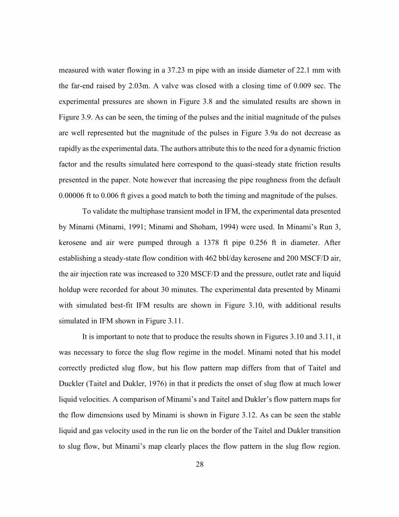
28

measured with water flowing in a 37.23 m pipe with an inside diameter of 22.1 mm with

the far-end raised by 2.03m. A valve was closed with a closing time of 0.009 sec. The

experimental pressures are shown in Figure 3.8 and the simulated results are shown in

Figure 3.9. As can be seen, the timing of the pulses and the initial magnitude of the pulses

are well represented but the magnitude of the pulses in Figure 3.9a do not decrease as

rapidly as the experimental data. The authors attribute this to the need for a dynamic friction

factor and the results simulated here correspond to the quasi-steady state friction results

presented in the paper. Note however that increasing the pipe roughness from the default

0.00006 ft to 0.006 ft gives a good match to both the timing and magnitude of the pulses.

To validate the multiphase transient model in IFM, the experimental data presented

by Minami (Minami, 1991; Minami and Shoham, 1994) were used. In Minami’s Run 3,

kerosene and air were pumped through a 1378 ft pipe 0.256 ft in diameter. After

establishing a steady-state flow condition with 462 bbl/day kerosene and 200 MSCF/D air,

the air injection rate was increased to 320 MSCF/D and the pressure, outlet rate and liquid

holdup were recorded for about 30 minutes. The experimental data presented by Minami

with simulated best-fit IFM results are shown in Figure 3.10, with additional results

simulated in IFM shown in Figure 3.11.

It is important to note that to produce the results shown in Figures 3.10 and 3.11, it

was necessary to force the slug flow regime in the model. Minami noted that his model

correctly predicted slug flow, but his flow pattern map differs from that of Taitel and

Duckler (Taitel and Dukler, 1976) in that it predicts the onset of slug flow at much lower

liquid velocities. A comparison of Minami’s and Taitel and Dukler’s flow pattern maps for

the flow dimensions used by Minami is shown in Figure 3.12. As can be seen the stable

liquid and gas velocity used in the run lie on the border of the Taitel and Dukler transition

to slug flow, but Minami’s map clearly places the flow pattern in the slug flow region.

29

Since Taitel and Dukler’s map has been much more widely used, no attempt was made to

adjust the flow pattern determination algorithm in the IFM software, but the flow pattern

was manually forced to slug flow for this prediction.

Note that the simulated results show a great similarity to the experimental data. It

should be noted that the liquid holdup dropped by about 2%, the pressure at Station 1 (209

ft in the model) rose about 5 psi, and the peak pressure at Station 1 rose about 9 psi in both

the model and the experiment. As a result of the comparison, it was concluded that the pipe

flow algorithms are adequate for use in field-scale simulations.

30

Figure 3.1. Schematic of Superposition used for Annular Flow.

Figure 3.2. Schematic of flow regimes in vertical flow, (a) bubbly flow, (b) slug flow, (c) churn flow, (d) annular flow, (e) disperse bubbly flow (adopted from Shirdel, 2013).

Figure 3.3. Schematic of flow regimes in horizontal flow, (a) stratified flow, (b) bubbly flow, (c) slug flow, (d) annular flow (adopted from Shirdel, 2013).

31

Figure 3.4. Flow pattern map for vertical flow (adopted from Shirdel, 2013).

Figure 3.5. Flow pattern map for horizontal flow (adopted from Shirdel, 2013).

Figure 3.6. Schematic of grid used in solution of momentum and energy equations.

32

Figure 3.7. Schematic of grid used in solution of mass equations.

Figure 3.8. Water hammer experimental data from Bergant et al. (2001), Figure 2.

a b

Figure 3.9. Water hammer predictions (a) Roughness = 0.00006 ft, (b) Roughness = 0.006 ft.

33

Figure 3.10. Multiphase experimental data Run 3 from Minami’s dissertation with best-fit IFM calculation (Minami, 1991).

Figure 3.11. Simulated Minami Run 3 (Minami, 1991).

34

Figure 3.12. Comparison of Minami (Minami, 1991) and Taitel & Dukler (Taitel and Dukler, 1976) flow regime maps.

35

Chapter 4: Multiphase Separators

Within the surface facilities, fluid separation plays an important role in producing

saleable oil, ensuring that the disposal water does not contain significant amounts of oil

and that water does not carry over into the gas sales line. Separation systems also determine

to some extent the quality of sales oil and gas. As such, it is important to be able to model

separators in order to optimize the production and the value of production from wells, as

well as the quality of the water that will be disposed of or re-injected. In the industry a

variety of separators are used, ranging from vertical and horizontal separators relying on

gravity to segregate the fluids, to vortex separators that use centrifugal forces to accelerate

the separation process. Separators may also contain coalescing plates and other

mechanisms that cause droplets to coalesce more rapidly.

An overview of separator characteristics and operation is provided by Langston

(2003) and separator design is explained by Arnold and M. Stewart (1999). Separator

design is usually based on consideration of worse case scenarios wherein the residence

time is selected to ensure that droplets of a certain size are able to rise or fall and coalesce

before fluids exit the separator. While this is sufficient for separator design and sizing, it

provides little insight into the dynamic behavior of a separator, nor does it allow

quantifying the effect of exceeding the separator design capacity.

Several authors have presented detailed models of separators based on

Computational Fluid Dynamics (CFD) and the dynamics of droplet size distributions.

Examples of these modeling efforts have been presented in the literature. See Frankiewicz

and Lee (2002); Hafskjols et al. (1999); Hallinger et al. (1996); Song et al. (2010). In

general these models appear to be computationally intensive and not directly suitable for

36

inclusion in an integrated model that also includes many other computationally intensive

modules.

For that reason, a simplified model of gravity separators was developed for use in

the integrated field model. Since gravity separators are the most common type of separator

used in marginal field applications, work was focused on modeling the operation of vertical

gravity separators using basic physics to honor the gravitational segregation process and

obtain a dynamic model of separator performance. In the case of gravity segregation, the

process is based on the application of Stokes’ Law, Bird et al. (2007), for drop motion.

VERTICAL SEPARATOR

The most common separator used in marginal oil fields is probably a vertical

gravity separator known as “wash tank” or “gun barrel.” It consists of a gas separation unit

at the inlet that allows gas to flow directly to the gas handling system and a large vertical

tank where oil and water separate due to gravity. The oil and water enter the separator

through an inlet pipe usually terminated in a serrated plate that forces the oil and water

mixture to spread out across the tank’s cross section. An oil outlet is located well above

the inlet and a water outlet is located near the base of the separator. A schematic diagram

of a vertical separator is shown in Figure 4.1. Due to the density difference between gas

and liquids, gas separation is not usually a concern; so the effort in this work has focused

on modeling the separation of oil and water.

Fundamental Equations

The fundamental relation that describes gravity segregation is Stokes’ Law, which

describes the terminal velocity of a spherical drop that rises or falls through a liquid of a

different density. For the purposes of separator modeling, Stokes’ Law can be stated as

Equation 4.1 (Arnold, 1999), where is the density difference between the fluids (lb/ft3),

37

d is the droplet diameter (micron), and is the viscosity of the continuous phase (cp).

Velocity can increase due to large density differences, large drop sizes and lower viscosity

of the continuous phase.

𝑣𝑡 =1.11𝑥10−6∆𝜌𝑑2

𝜇 .............................................................................................. (4.1)

To model a vertical separator an approach similar to that presented by Rosso and

Sona (2001) is taken. Rosso and Sona considered simplified volume fraction distributions

and attempted to solve the resulting equations analytically, but for the purpose of general

separator modeling a more flexible and general approach is needed, whereby the volume

fraction distributions are general and sources and sinks must be considered to represent the

inflow and outflow of fluids from the separator.

For detailed modeling, it is assumed that the velocity in the separator is low enough

that transient velocity effects can be neglected. Under that assumption, it is apparent that

the inlet flow must divide between the oil outlet and the water outlet. In the ideal case, it

can be assumed that the downward volumetric flow toward the water outlet is equal to the

volumetric inflow of water and, conversely, the upward volumetric flow of fluids toward

the oil outlet is equal to the volumetric inflow of oil. This is expressed in the following

equations, where subscript s represents standard conditions.

𝑣𝑇+ =𝑞𝑠𝑜

𝐴

𝜌𝑠𝑜

𝜌𝑜 and 𝑣𝑇− =

𝑞𝑠𝑤

𝐴

𝜌𝑠𝑤

𝜌𝑤 ....................................................................... (4.2)

Normally water would flow downward relative to oil due to gravity. Using the oil

velocity as a reference, the water velocity can be expressed as the oil velocity less the water

relative velocity determined from Stokes’ law. To maintain a volumetric balance, the total

velocity can also be expressed in terms of oil and water velocities as follows.

𝑣𝑤 = 𝑣𝑜 − ∆𝑣 ........................................................................................................ (4.3)

𝑣𝑇 = (1 − 𝑓𝑤)𝑣𝑜 + 𝑓𝑤𝑣𝑤 ...................................................................................... (4.4)

38

Substituting and rearranging yields an expression for the oil and water velocities in terms

of the total velocity and the relative velocity difference.

𝑣𝑜 = 𝑣𝑇 + 𝑓𝑤∆𝑣 .................................................................................................... (4.5)

𝑣𝑜 = 𝑣𝑇 − (1 − 𝑓𝑤)∆𝑣 ......................................................................................... (4.6)

During operation of the separator, a constant operating pressure is assumed to be

maintained above the liquid. For steady state, that implies a constant gas volume and

therefore, if the gas separation is assumed to be perfect, the gas inflow will be equal to the

gas outflow.

To compute the pressure distribution within the separator, the total liquid density is

integrated from the liquid level downward. This is expressed as Equation 4.7.

𝑝(𝑧) = 𝑝𝑔𝑎𝑠 + ∫ [(1 − 𝑓𝑤)𝜌𝑜 + 𝑓𝑤𝜌𝑤]𝑑𝑧𝑧𝑔𝑎𝑠

𝑧 .......................................... (4.7)

Finally, it is also necessary to compute the changes in the distribution of the volume

fraction of fluids based on a mass balance of one of the phases. Choosing water to be

consistent with the balance equations used in pipe flow, the mass balance equation can be

written as:

𝜕

𝜕𝑡(𝑓𝑤𝜌𝑤) +

𝜕

𝜕𝑧(𝑓𝑤𝜌𝑤𝑣𝑤) −

𝑞𝑠𝑤𝜌𝑠𝑤

𝐴 ∆𝑧= 0 ........................................................... (4.8)

where qsw represents a source of fluids entering the separator per unit height. Normally this

term will be zero, except at the inlet and the outlet to the separator. It should also be noted

that inlet flow rates are positive, while outlet flow rates will be negative in this formulation.

Temperature in the separator is evaluated using an energy balance equation similar

to Equation 3.10 for pipe flow. Since the velocity within the separator is generally very

low and dominated by gravity, the pressure gradient and gravity terms cancel and the

kinetic energy term is assumed to be insignificant. In terms of internal energy, e, the energy

balance can be written as:

39

𝜕

𝜕𝑡(𝑓𝑤𝜌𝑤𝑒𝑤 + 𝑓𝑜𝜌𝑜𝑒𝑜) +

𝜕

𝜕𝑧(𝑓𝑤𝜌𝑤𝑒𝑤𝑣𝑤 + 𝑓𝑜𝜌𝑜𝑒𝑜𝑣𝑜)

− 𝑞𝑠𝑤𝜌𝑠𝑤𝑒𝑠𝑤+𝑞𝑠𝑜𝜌𝑠𝑜𝑒𝑠𝑜

𝐴 ∆𝑧+ 𝑈𝑆(𝑇 − 𝑇𝑒𝑥𝑡) = 0 ................................................ (4.9)

The energy relation can be simplified by expanding the partial derivatives,

substituting the mass balance equations for both oil and water and expressing the

derivatives of the internal energy as heat capacity multiplied by temperature derivatives.

In this form, the equation becomes:

(𝑓𝑤𝜌𝑤𝑐𝑝𝑤 + 𝑓𝑜𝜌𝑜𝑐𝑝𝑜)𝜕𝑇

𝜕𝑡+ (𝑓𝑤𝜌𝑤𝑐𝑝𝑤𝑣𝑤 + 𝑓𝑜𝜌𝑜𝑐𝑝𝑜𝑣𝑜)

𝜕𝑇

𝜕𝑧

− 𝑞𝑠𝑤𝜌𝑠𝑤𝑐𝑝𝑠𝑤+𝑞𝑠𝑜𝜌𝑠𝑜𝑐𝑝𝑠𝑜

𝐴 ∆𝑧(𝑇 − 𝑇𝑠) + 𝑈𝑆(𝑇 − 𝑇𝑒𝑥𝑡) = 0 ............................. (4.10)

Numerical Solution

Solutions of the equations representing separator behavior are straightforward,

except for the determination of the relative phase velocity from Stokes’ law and the

determination of the water volume fraction from the mass balance equation, which will be

discussed in more detail.

At each time step the total velocity above and below the inlet height is calculated

with equation 4.2, and then Equations 4.5 and 4.6 are used directly to compute the velocity

of oil and water phases, respectively.

The volume fraction of water in each vertical cell is computed from the mass

balance for water in Equation 4.8 using an implicit formulation and weighting based on the

direction of volume fraction change. Since the formulation is nonlinear, the following

difference equation is used and a Newton iteration is performed by evaluating the Jacobian.

Note that the terms in braces depend on the direction of the weighting.

40

𝑔𝑖 = 𝑓𝑤𝑖𝑛 𝜌𝑤𝑖

𝑛 − 𝑓𝑤𝑖𝑛−1𝜌𝑤𝑖

𝑛−1 +∆𝑡

∆𝑧{

𝑓𝑤𝑖𝑛 𝜌𝑤𝑖

𝑛

or𝑓𝑤𝑖+1

𝑛 𝜌𝑤𝑖+1𝑛

} 𝑣𝑤𝑖𝑛 −

∆𝑡

∆𝑧{𝑓𝑤𝑖−1

𝑛 𝜌𝑤𝑖−1𝑛

or𝑓𝑤𝑖

𝑛 𝜌𝑤𝑖𝑛

} 𝑣𝑤𝑖−1𝑛

− 𝑞𝑠𝑤𝜌𝑠𝑤

𝐴

∆𝑡

∆𝑧= 0 ............................................................................................. (4.11)

where the exponent, n, represents the time step.

When the volume fraction of water has been determined, the updated pressure

distribution in the separator is evaluated with Equation 4.7 using the trapezoidal rule and

the phase densities are updated.

Finally, a heat balance is performed to determine the temperature distribution using

the energy equation in the form of Equation 4.10. As for the mass balance, an implicit finite

difference scheme is used and the Jacobian is computed for an iterative solution. The finite

difference once again depends on weighting and is expressed as follows:

ℎ𝑖 = 𝜌𝐿𝑖𝑛 𝑐𝑝𝐿𝑖

𝑛 (𝑇𝑖𝑛 − 𝑇𝑖

𝑛−1) +∆𝑡

∆𝑧𝜌𝐿𝑖

𝑛 𝑐𝑝𝐿𝑖𝑛 𝑣𝐿𝑖

𝑛 {𝑇𝑖

𝑛 − 𝑇𝑖−1𝑛

or𝑇𝑖+1

𝑛 − 𝑇𝑖𝑛

}

− 𝑞𝑠𝐿𝜌𝑠𝐿𝑐𝑝𝑠𝐿

𝐴

∆𝑡

∆𝑧(𝑇𝑖

𝑛 − 𝑇𝑠𝑖𝑛) + 𝜋𝐷𝑈(𝑇𝑖

𝑛 − 𝑇𝑒𝑥𝑡𝑛 ) = 0 .................................. (4.12)

41

Figure 4.1. Schematic of a typical vertical separator.

vi-1

vi

pi-1,

Ti-1,

HLi-1,

fwi-1

pi+1,

Ti+1,

HLi+1,

fwi+1

pi,

Ti,

HLi,

fw

Mom/Energy

Mass

Balance

42

Chapter 5: Well Model

It seems obvious that nearly all fluids flowing in an oil field come from wells, so

representing well performance is an important part of the overall field modeling. In order

to model well performance, it is also necessary to consider the inflow of fluids from the

reservoir and the detailed wellbore dynamics accounting for artificial lift methods. For the

purpose of the full field model documented in this work, two cases are considered. In the

first case, for testing purposes, a constant rate well is modeled, while for more practical

situations, the case of a beam pumped well typically used in marginal oil fields is modeled.

CONSTANT RATE WELL

In order to test the software, it is convenient to have a constant rate source. While

the equation for a constant rate source is simple, when considering transient flow, large

magnitude transient pressures arise during the simulation. These transients are analogous

to the well-known “water hammer” phenomenon; for example, as measured by Bergant et

al. (2001). In order to more realistically represent field conditions of valves opening in a

finite time, a valve time parameter, tv, is defined and the flow rises in a sinusoidal manner

over the length of the valve opening time. In the software, a default value of 1 second is

applied. The resulting equation for the rate is shown in Equation 5.1 and the rate is shown

in Figure 5.1.

𝑞𝑗 = {

𝑞𝑗 𝑖𝑛𝑝𝑢𝑡

2[1 + sin (

𝜋𝑡

∆𝑡𝑣−

𝜋

2)] 𝑡 < ∆𝑡𝑣

𝑞𝑗 𝑖𝑛𝑝𝑢𝑡 𝑡 ≥ ∆𝑡𝑣 ................................................................. (5.1)

43

BEAM PUMPS

Rod pumps are normally modeled using the damped wave equation, which is

derived by applying Newton’s equation for motion to infinitesimal segments of the rods

and considering forces due to stress in the rods and drag forces due to fluid drag and

assuming that rod stretch is represented by using a Young’s modulus to relate stress and

strain in the rods. Early analyses of rod pump behavior used trial and error approaches, and

then analog computers were used to solve the resulting wave equations. A more complete

history and literature review of historical rod pump modeling has previously been

presented by several authors (cf. Lekia and Evans, 1995), but most of the recent models

can be traced back to Gibbs (1963), where a numerical solution to the damped wave

equation was presented. Methods for solving the equations presented by Gibbs are

presented by several authors (cf. Gibbs and Neely, 1966; Schafer and Jennings, 1987);

however, use of the Gibbs formulation requires estimation of the empirical damping factor

which may be difficult. In fact some authors (cf. Schafer, 1987) suggest that different

damping factors should be used on the upstroke and downstroke calculations.

Various authors have extended the Gibbs model. Csaszar et al. (1991) added the

effect of fluid inertia to the basic model and showed that it may affect the results under

some conditions. Doty and Schmidt (1983) added fluid drag to the rod motion equations

by using friction factor correlations from Valeev and Repin (1976) to represent the drag

effects and reported the effects of both fluid inertia and rod and coupling drag on the

calculated rod loads. Lekia (1995) followed a similar procedure to account for rod drag

using fluid flow models with an additional drag force due to rod couplings represented by

the Valeev and Repin (1976) friction factors, but his multiphase model assumed

homogeneous, no-slip, bubble flow. Later Barreto Filho (2001) accounted for a variable

fluid level on the downhole pump and used the Valeev (1976) friction factors for rod

44

coupling drag, but assumed single phase laminar flow in the rod and tubing annulus. Xu et

al. (1999) later extended the rod pump model to incorporate Coulomb friction due to the

rods rubbing on the tubing due to well deviation, and also coupled multiphase flow through

the use of friction factors determined using computational fluid dynamics.

Besides the rod drag and the fluid formulation, very little other works appears to

have been done on representing the boundary conditions required for solution of the

equations of motion. Most rod pump models have assumed constant tubing pressure (cf.

Lekia, 1995) or pump plunger load and have ignored transient reservoir flow effects. A

steady-state reservoir inflow model was used by Barreto Filho (2001) to account for

variations in fluid level and pump intake pressure, but most other authors have ignored the

effect of reservoir transients and coupling of the tubing to a surface flow system. Figure

5.2 shows pressure fluctuations measured at the tubing on a beam pumping well by

Pennebaker (2014). Although the pressure scale is calibrated in analog-digital converter

voltage, the scale is linear and indicates a fluctuation from a low of about 50 psi and peaks

of about 150 psi. Since the stroke rate was reported to be 6 SPM, it is apparent that there

are two peaks during each rod cycle. Personal experience also indicates that tubing pressure

fluctuations are commonly observed on rod pump wells, although they are rarely reported

due to gauge inertia and not recorded at a high enough sampling frequency.

As a result of these considerations, a more complex rod pump modeling system has

been developed which removes the empirical damping factor from the rod drag

calculations, couples fluid friction and rod drag forces, represents transient flow throughout

the system, and couples the rod pump model to a transient flow reservoir model. Since this

system allows the evaluation of the various effects that have been neglected in previous

models, it can be used to determine when it is valid to ignore the neglected effects, and also

45

allows the evaluation of new diagnostics and analytical procedures that make use of the

transient system behavior.

Rod Motion

In this work a generalized force and momentum balance on the rod string is used to

determine the equation of motion describing the rod behavior. This is the same approach

used by both Lekia (1995) and Barreto Filho (2001). The partial differential equation for

rod motion is shown in Equation 5.2.

𝜕2𝑢

𝜕𝑡2 = 𝐸𝑟

𝜌𝑟

𝜕2𝑢

𝜕𝑥2 + 𝑔 − (𝐹𝑎𝐿 + 𝐹𝑎𝐺) +𝑃

𝜌𝑟𝐴𝑟

𝑑𝐴𝑟

𝑑𝑥 ..................................................... (5.2)

where

u = rod velocity (ft/sec)

x = distance (ft)

Er = Young’s modulus for rod material (psi)

Ar = Cross sectional area of rods (ft2)

g = acceleration due to gravity (ft/sec/sec)

FaL drag force on rods due to liquid (lbf/ft)

FaG drag force on rods due to gas (lbf/ft)

P = pressure (psia)

x = distance along unstressed rods (ft)

r = density of rod material (lb/ft3)

Gibbs (1963) used an empirical damping factor to account for drag forces, where

the drag force is proportional to the rod velocity. In this work we use a friction factor

formulation for flow in pipes to couple the fluid friction to the drag forces on the rods; thus

the rod drag forces per unit length are described by the FaL and FaG terms in the pipe flow

momentum equations documented in Chapter 3. This approach ensures consistency in the

46

pressure drop due to flow with the corresponding rod drag forces; it has previously been

presented by Lekia (1995) for single phase and multiphase flow and by Barreto Filho

(2001) for single phase laminar flow.

At first thought, it would appear that the normal pipe friction terms could be used

to describe drag on the rods in the tubing rod annulus. However, it is important to note that

the pipe friction relations based on Reynolds number and roughness also assume uniform

flow along the length of the pipe, but in the rod tubing annulus the flow is not uniform due

to restrictions caused by the rod couplings. Friction factors for flow in the rod-tubing and

coupling-tubing annulus were presented by Valeev and Repin (1976) and used by both

Lekia (1995) and by Barreto Filho (2001) in their models. In this work we also use the

Valeev and Repin friction factors and apply them in a manner equivalent to that of Barreto

Filho, whereby the tubing and rod friction loss is modified by a factor depending on the

additional losses imposed by the rod couplings. The following relations are used for liquid

flow and the analogous relation is used for gas. The effect of any rod centralizers is ignored.

𝐹𝑎𝐿′ = 𝐹𝑎𝐿𝐷𝑡 [1 +

52000(𝐷𝑐𝐷𝑡

−0.381)2.57

{2.77±1.69𝑅𝑒𝐿

′

𝑅𝑒𝐿}

96

𝑅𝑒𝐿[1±

𝑅𝑒′

𝑅𝑒(0.2+0.39

𝐷𝑟𝐷𝑡

)]] ............................................ (5.3)

𝑅𝑒𝐿 =𝜌𝐿𝑣𝐿(𝐷𝑡−𝐷𝑟)

𝜇𝐿 , 𝑅𝑒𝐿

′ =𝜌𝐿𝑣𝑟(𝐷𝑡−𝐷𝑟)

𝜇𝐿 ............................................................... (5.4)

where

L = density of liquid (lb/ ft3)

L = viscosity of liquid (cp)

Dt = tubing diameter (ft)

Dc = coupling diameter (ft)

Dr = rod diameter (ft)

FaL = drag force on rods due to liquid (lbf/ft)

47

FaG = drag force on rods due to gas (lbf/ft)

REl = Reynolds number for liquid flow

𝐹𝑎𝐺′ = 𝐹𝑎𝐺𝐷𝑡 [1 +

52000(𝐷𝑐𝐷𝑡

−0.381)2.57

{2.77±1.69𝑅𝑒𝐺

′

𝑅𝑒𝐺}

96

𝑅𝑒𝐺[1±

𝑅𝑒𝐺′

𝑅𝑒𝐺(0.2+0.39

𝐷𝑟𝐷𝑡

)]

] ........................................... (5.5)

𝑅𝑒𝐺 =𝜌𝐺𝑣𝐺(𝐷𝑡−𝐷𝑟)

𝜇𝐺 , 𝑅𝑒𝐺

′ =𝜌𝐺𝑣𝑟(𝐷𝑡−𝐷𝑟)

𝜇𝐺 ............................................................. (5.6)

Given the fundamental rod motion equation, the equation is converted to finite

difference form for numerical solution. The methods used by Gibbs (1963) and by Everitt

and Jennings (1992) are modified in this work to derive an explicit rod motion calculation

whereby the time step is not assumed to be constant. Since two time levels are required to

approximate the second derivative with respect to time, this allows automatic time step

adjustments while the model is running. The resulting explicit finite difference equation is

as follows.

𝑢𝑖𝑛+1 = [(𝐴𝑟𝑖+1𝑢𝑖+1

𝑛 − 2𝐴𝑟𝑖𝑢𝑖𝑛 + 𝐴𝑟𝑖−1𝑢𝑖−1

𝑛 )𝑎2∆𝑡𝑛(∆𝑡𝑛+∆𝑡𝑛−1)

2∆𝑥2

+(∆𝑡𝑛+∆𝑡𝑛−1)

∆𝑡𝑛−1𝐴𝑟𝑖𝑢𝑖

𝑛 −∆𝑡𝑛

∆𝑡𝑛−1𝐴𝑟𝑖𝑢𝑖

𝑛−1

−𝐴𝑡

𝜌𝑟𝑔𝑐𝐴𝑟𝑖(𝐹𝑎𝐿𝑖 + 𝐹𝑎𝐺𝑖)

∆𝑡𝑛(∆𝑡𝑛+∆𝑡𝑛−1)

2]/𝐴𝑟𝑖

............................. (5.7)

where

u = rod velocity (ft/sec)

Ar = rod cross sectional area (ft2)

Initial and boundary conditions are also required for the solution of the rod string

motion. The initial condition is computed by assuming the rods are hanging in static

equilibrium with the stress and the corresponding strain computed from the buoyant rod

weight at each point in the rod string. The boundary conditions consist of the polish rod

position at each time step, u[0,t], as well as the load at the pump computed from the tubing

flow and downhole pump pressure relations described below.

48

Surface Pumping Unit

In this study the Gray (1963) pumping unit model is used whereby the motion is

represented by a 4 bar problem with the driven element (R in Figure 5.1) rotating at a

constant rate.. Standard API unit dimensions are used throughout, and a constant angular

velocity of element R in Figure 5.1 is assumed. Future work should incorporate motor

slippage but is not considered here. Using API pumping unit geometry nomenclature, the

relations are as follows:

𝐿2 = √(𝐻 − 𝐺)2 + 𝐼2 ........................................................................................ (5.8)

𝐶1 = cos(𝜃 + 𝜃𝑐) ............................................................................................... (5.9)

𝐶2 = √1 + (𝑅

𝐿2)

2

+ 2𝐶1𝑅

𝐿2 ............................................................................... (5.10)

𝐶3 =1

𝐶2(𝑎𝑎 +

𝑅𝐶1

𝐶) ........................................................................................... (5.11)

𝐶4 =𝑅 sin(𝜃+𝜃𝑐)

𝐶2𝐿2 ................................................................................................. (5.12)

𝑎𝑎 =𝑅2+𝐿2

2+𝐶2−𝑃2

2𝐿2𝐶 ............................................................................................. (5.13)

𝛼 = tan−1 (𝐶4

√1−𝐶42) ......................................................................................... (5.14)

𝛽 = cos−1(𝐶3) ................................................................................................. (5.15)

𝑥0 =1

12[𝐴(𝛼 + 𝛽) − 𝑥𝑚𝑖𝑛] ............................................................................. (5.16)

𝜃𝑛 = 𝜃𝑛−1 +2𝜋∆𝑡𝑛

60 𝑆𝑃𝑀⁄ ........................................................................................ (5.17)

The surface polish rod position is advanced by assuming a constant angular

velocity, whereby 2 radians are traversed during each stroke. The surface position shown

as x0 in Equation 5.16 is the surface position of the rod string at the new time step, u[0,tn].

49

Downhole Pump

The downhole pump is modeled using a simple mass balance to determine pump

pressure. Variation of pressure with position inside the pump and plunger inertia are not

considered; complete separation of gas before entry into the pump is not assumed in the

models presented here. The internal pump volume depends on the plunger position which

is equal to the bottom of the rod string. Since the fluid properties depend on pressure, the

pump pressure is determined by searching for the root of Equation 5.18.

𝑉𝑝𝑛 = 𝑉𝑝

𝑛−1 + (𝑢𝐿𝑛 − 𝑢𝐿

𝑛−1) = 𝑉𝑜𝑛𝐵𝑜 + 𝑉𝑤

𝑛𝐵𝑤 + (𝑉𝑔𝑛 − 𝑅𝑠𝑉𝑜

𝑛) ..................... (5.18)

Once the internal pump pressure is known, the load on the plunger can be computed

by the pressure difference between the tubing pressure above the pump and the internal

pump pressure, multiplied by the net plunger area. This serves as a load boundary condition

on the bottom of the rod string, whose equation of motion was previously described.

𝜕𝑢𝐿𝑛

𝜕𝑥=

𝐴𝑝(𝑝𝑡𝑁𝑛 −𝑝𝑝

𝑛)

𝐸𝑟𝐴𝑝 .............................................................................................. (5.19)

In addition, the pump plunger motion provides a boundary condition for mass flow

into the bottom of the tubing. During the upstroke the plunger moves upward and the

volumetric flow into the bottom of the tubing is equal to the area of the pump-rod annulus

times the plunger velocity, and the volumetric flow into the pump from the wellbore is

equal to the plunger area times the plunger velocity. Similarly, during the down stroke, the

rods displace fluids inside the pump barrel, so the volumetric flow into the base of the

tubing is equal to the rod area times the plunger velocity. During the stroke, the traveling

and standing valves states (open or closed) are determined based on the pressure difference

between the internal pump and the tubing pressure or the external wellbore pressure.

50

CASING ANNULUS

In the casing, it is assumed that there is no net liquid flow inside the casing tubing

annulus and that gas is bubbling through a static liquid column. The correlation presented

by Gilbert (1954) is used to determine the liquid and gas volume fraction in the gaseous

liquid column. The fluid mass inside the casing is computed from the reservoir flow

equation and a superficial gas velocity is thereby determined. Above the perforations, there

is a gaseous liquid column with a liquid holdup determined from Gilbert’s correlation

(Gilbert, 1954) using the superficial gas velocity. Above the gaseous liquid column, free

gas is assumed to go to the surface. The volume of oil water and gas is computed from

mass balance and if constant surface casing pressure is specified, the volume of gas to the

fluid level is computed, so that the bottom hole pressure of the fluid column is equal to the

reservoir pressure. If a closed annulus is specified, the surface pressure is found by

searching for the root of the volume balance using pressure dependent fluid properties.

Fluid from the gaseous liquid column flows into the pump based on the plunger

velocity and pump area, and the volumetric flow into the pump from the casing annulus,

therefore both liquid and free gas may enter the pump. Similarly, during the down stroke,

the rods displace fluids inside the pump barrel, so the volumetric flow into the base of the

tubing is equal to the rod area times the plunger velocity. During the stroke, the traveling

and standing valves states (open or closed) are determined based on the pressure difference

between the internal pump and the tubing pressure or the external wellbore pressure.

When the traveling valve is open on the downstroke, it is assumed that free gas

inside the pump will enter the tubing first and liquids will enter only when all the free gas

has been depleted from the pump. It is important to note that in most of the cases presented

later in this dissertation, no free gas is found in the pump since the pressure is generally

above the bubble point pressure and all gas is in solution.

51

RESERVOIR AND COMPLETION MODEL

To represent transient fluid flow from the reservoir into the wellbore a radial flow

reservoir model similar to that used in pressure transient analysis is used as presented by

Earlougher (1977) among others. The reservoir model includes skin at the wellbore and

relates the fluid flow into the well to the pressure distribution in the near well area.

1

𝑟

𝜕

𝜕𝑟(𝑟

𝜕𝑝

𝜕𝑟) =

0.000264𝑘

𝜑𝜇𝑐𝑡𝑟𝑤2

𝜕𝑝

𝜕𝑡 ................................................................................. (5.20)

𝑝𝑤 = 𝑝𝑟𝑤−

𝑘ℎ

141.2𝐵𝑜𝜇𝑆 (𝑟

𝜕𝑝

𝜕𝑟)

𝑟=𝑟𝑤

................................................................... (5.21)

𝑞𝑜 =𝑘ℎ

141.2𝐵𝑜𝜇(𝑟

𝜕𝑝

𝜕𝑟)

𝑟=𝑟𝑤

.................................................................................. (5.22)

𝑞𝑔 = 𝑅𝑞𝑜.......................................................................................................... (5.23)

𝑞𝑤 =𝑓𝑤

1−𝑓𝑤𝑞𝑜 ................................................................................................... (5.24)

𝑞𝑜𝑡𝑛 = {

(1 − 𝑓𝑤)𝑑𝑉𝑝

𝑑𝑡𝐵𝑜 (𝑉𝑔

𝑛 − 𝑅𝑠𝑉𝑜𝑛) ≤ 0

0 (𝑉𝑔𝑛 − 𝑅𝑠𝑉𝑜

𝑛) > 0 ................................................... (5.25)

𝑞𝑤𝑡𝑛 = {

𝑓𝑤𝑑𝑉𝑝

𝑑𝑡𝐵𝑤 (𝑉𝑔

𝑛 − 𝑅𝑠𝑉𝑜𝑛) ≤ 0


𝑛) > 0 ............................................................ (5.26)

𝑞𝑔𝑡𝑛 = {

𝑑𝑉𝑝

𝑑𝑡𝐵𝑔 (𝑉𝑔

𝑛 − 𝑅𝑠𝑉𝑜𝑛) > 0


𝑛) ≤ 0 .................................................................. (5.27)

In contrast to normal pressure transient testing, a pressure boundary condition is

applied at the wellbore, whereby the flow into the well is controlled by the pressure inside

the wellbore. Since the pressure varies with pump action and annular fluid level, a constant

or steady state flow rate will never be reached in general.

52

Figure 5.1. API pumping unit geometry parameters.

Figure 5.2. Rate variation due to valve opening.

0.0

0.2

0.4

0.6

0.8

1.0

0.0 0.5 1.0 1.5 2.0

q/q

inp

ut

t/tv

Rate Due to Valve Opening

53

Figure 5.3 Tubing pressure variation measured on a beam pumping well (Pennebaker, 2014).

0

5

10

15

20

25

30

35

40

45

0 5 10 15 20 25 30 35 40 45 50 55 60 65

AD

C u

nit

s (

rela

tive

)

Time (secs)

54

Chapter 6: Auxiliary Flow Equipment

Within the surface facilities a variety of flow equipment is needed to handle,

transfer, and store produced fluids. These include tanks, flow junctions (i.e. headers),

pumps, chokes, and compressors. In IFM these items are not modeled in detail internally

but are represented as steady-state flow items.

FLOW JUNCTIONS

In general, the flow streams go to a junction, or header, where the flows are

combined before being routed to a separator or other facility for treatment. Since the total

volume of fluids within a header is usually very small compared to the flow rate through

the header, steady-state flow within the header is assumed and pressure is assumed to be

continuous, so that all incoming and outgoing streams will have the same pressure.

Temperature is computed by performing a heat balance on the incoming streams to

compute an average temperature, which is assigned to all of the outgoing streams. When

more than one outgoing stream exist, the flow rates are divided equally among them. The

equations describing the flow junction are as follows, where the index i represents inlets 1

… n, and j represents outlets 1 … m, and p represents the component or phase.

𝑝𝑖 = 𝑝𝑗 , 𝑓𝑜𝑟 𝑎𝑙𝑙 𝑖𝑛𝑙𝑒𝑡𝑠 𝑖 𝑎𝑛𝑑 𝑜𝑢𝑡𝑙𝑒𝑡𝑠 𝑗 ............................................................ (6.1)

𝑞𝑝𝑗𝜌𝑝0 =1

𝑚∑ 𝑞𝑝𝑖𝜌𝑝0

𝑛𝑖=1 , 𝑓𝑜𝑟 𝑒𝑎𝑐ℎ 𝑜𝑢𝑡𝑙𝑒𝑡𝑠 𝑗, 𝑒𝑎𝑐ℎ 𝑝ℎ𝑎𝑠𝑒 𝑝 .......................... (6.2)

𝑇𝑗 =∑ 𝑇𝑖(𝑞𝑝𝑖𝜌𝑤0𝑐𝑝𝑤𝑐𝑝𝑔)𝑛

𝑖=1

∑ (𝑞𝑝𝑖𝜌𝑝𝑤0𝑐𝑝𝑜𝑐𝑝𝑔)𝑛𝑖=1

, 𝑓𝑜𝑟 𝑒𝑎𝑐ℎ 𝑜𝑢𝑡𝑙𝑒𝑡𝑠 𝑗 .................................................. (6.3)

55

TANKS

Tanks are important for temporary storage of fluids within a field facility. Since the

flow velocity is generally very slow and a tank normally has no outlet, only storage of

fluids in the tanks is modeled in IFM. Pressure is assumed to be static and temperature is

assumed to be uniform, representing a well-mixed fluid system at all times. As a result, the

inlet pressure of the tank is equivalent to the static pressure head of fluids within the tank

and will increase as the amount of fluids increases. In addition, the temperature is

calculated by performing a heat balance on the tank fluids, plus the inlet fluids, accounting

for heat loss to the environment.

SURFACE PUMPS

Pumps are needed to boost the pressure of fluids traveling through the facilities

when the gravity head or well pressures are not adequate to allow flow through the entire

facility. In IFM pumps are modeled as steady-state devices, where the mass through the

pump is conserved. Each pump requires a performance relationship relating the flow rate

and the pressure increment to the power requirements.

COMPRESSORS

Just as pumps are commonly used to move fluids through a facility, compressors

are commonly used to move gases when the pressures are not adequate for processing

requirements. In IFM compressors are modeled as steady-state devices, where a mass

balance of fluids moving through the compressor is calculated. Due to the nature of gas,

compression is always accompanied by an increase in temperature, which normally must

be handled by cooling to avoid destruction of the compressor. Each compressor requires a

performance relationship to relate the flow rate and pressure increase to the power

requirements.

56

CHOKES

Chokes are used as control devices to limit flow and/or to reduce pressure in various

parts of the flow system. Chokes are commonly used at wells to avoid problems with surges

of fluids that may damage other equipment. In IFM chokes are modeled as steady-state

devices with the pressure drop computed from the flow rate through the choke, given its

orifice size. In addition, especially with gases, a temperature change may be observed. This

is computed using an adiabatic heat balance of fluids entering and leaving the choke, but

heat losses within the choke itself are not considered.

57

Chapter 7: Field Applications

Since the integrated field model has been developed and all of the parts have been

validated, it is of interest to apply the model to actual field cases. As shown in Figure 7.1

the predicted and the measured dynamometers for a well with 20o API oil are nearly

identical, even though no tuning or damping factor was attempted in the predicted

dynamometer card. Figure 7.2 also shows the predicted differences in dynamometer cards

due to differing oil API gravity. Although not attempted here, it appears that IFM can be

used to evaluate damping factors for use in damped wave equation applications by

predicting the dynamometer with IFM, then fitting it with a damped wave equation.

Figure 7.3 shows the fluid level change as the pump runs, while Figure 7.4 shows

the transient bottomhole pressure and oil flow rate from the reservoir influenced by the

drop in the fluid level and bottomhole pressure. As can be seen, there is no indication that

a stable pressure, flow rate or fluid level is achieved. Instead, fluctuations and transient

effects appear to continue. In fact, longer detailed simulations show that the well remains

in transient flow forever, since the pump strokes are shorter than the time needed for

transients to be damped. This seems to bring into question the normal assumptions of

constant rate and stable pump inlet pressure used in beam pump evaluations and designs.

Further work on that subject appears to be warranted to validate that steady-state

approximations can be used for design and diagnostics.

In most multi-well fields, flow from a number of wells goes to a flow junction, or

header, where the flows are combined before being routed to a separator or other facility

for treatment. To illustrate the effect of well interference through surface piping, a model

shown in Figure 7.5 comprising two beam pumped wells producing into a common header

was simulated. Pressure and rate fluctuations at the header are shown in Figures 7.6 and

58

7.7. Individual well fluctuations in pressure and rate are shown in Figure 7.8 and Figure

7.9. As can be seen, it appears that any assumption of steady-state flow is unwarranted,

even in a simple two-well facility as shown in Figure 7.5.

Figure 7.1. Predicted and measured dynamometer cards for 4,000 ft well.

Figure 7.2. Predicted dynagraph for 4,000 ft well. Difference in dynamometer response

due to differences in fluid density and viscosity, represented by API gravity differences.

• Damping Factor b = 0.6

• L = 4000 ft

• Dp = 2.5”

• Dr = 1”

• 10 SPM

0

5000

10000

15000

20000

25000

30000

0 1 2 3 4 5 6 7 8

Polish Rod Card

35oAP

I API

20o API

API

59

Figure 7.3. Predicted fluid level variation during startup of a beam pumped 4,000 ft well.

Figure 7.4. Predicted transient BHP and inflow rate for 4,000 ft well showing fluctuations

as the pump starts.

60

Figure 7.5. Comparison of measured and predicted dynamometers cards for 20 APIo and

4,000 ft well.

Figure 7.6. Predicted header pressure from example 2 well field.

Well 1 (6 SPM) 4,000’

Well 2 (5 SPM)

3000’

2” 10770’ flowline



61

Figure 7.7. Predicted header flow rate from example 2 well field

Figure 7.8. Predicted tubing pressure of wells in 2 well facility

Figure 7.9. Predicted wellhead rate of wells in 2 well facility

W1 W2

W1 W2

62

Conclusions and Recommendations

As a result of the work documented in this dissertation, the following conclusions

can be made and the following recommendations are made for future work.

CONCLUSIONS:

1) At the beginning of this work, it was doubtful that a complete field system could

be modeled fully in transient flow, due to the difficulty in solving the nonlinear

equations and the need for extremely small time steps for the surface

equipment; however it is now concluded that it is feasible to model wells and

simple facilities fully in transient flow.

2) Transient surface pressures exhibit complex behavior that may be chaotic.

3) As a result of the modeling work, it appears that common assumptions of

steady-state flow in wells and facilities are largely unwarranted and should be

reexamined when using simple analyses to estimate well performance and

facility behaviors.

4) Interference between wells through the surface facilities is apparent. Therefore,

interference-based analyses (interference tests, resistance capacitance models,

etc.) should not assume that all interference is through the reservoir.

RECOMMENDATIONS:

1) The model can be used to evaluate the use of damping factors in existing

damped wave equation software and analysis methods by generating

dynamometer cards using IFM, then fitting them with a damped wave equation

to determine the relationship between well and fluid properties and the apparent

damping factors.

63

2) The annular flow model used in this dissertation is different from standard

models, wherein a Reynolds number based on outer and inner radii is defined

and friction factors are determined from experiment. Further theoretical and

experimental work to further develop the superposition model used in this

dissertation is justified.

3) Figure 7.4 shows how seemingly chaotic behavior can arise in even a simple oil

field scenario. Chaos is defined by Hilborn et al. (1994) as a system that appears

to have a random component, but is actually deterministic and controlled by

nonlinear dynamics. The equations used in this dissertation are obviously

nonlinear and should be capable of showing chaotic behavior as in Figure 7.4.

It is known that chaotic systems tend to have solutions that follow an attractor

in a suitable parameter space. IFM can be used to determine the parameter space

and define the expected attractor. Then field measurements can be compared to

the expected attractor. Measurements differing from the expected might be

indicative of problems in the wellbore or surface facilities. This would provide

a useful tool for field surveillance. IFM could also be used to illustrate what

deviations are normal and arise from chaotic behavior and not from mechanical

problems.

4) The IFM well models should be extended to include progressive cavity pumps,

gas lift and electric submersible pumped wells.

5) Separator modeling in this dissertation is entirely empirical and should be

reevaluated, perhaps using CFD (computational fluid dynamics) to justify the

empirical approximations.

6) The rod coupling friction factors due to Valeev and Repin (1976) appear to be

generally accepted and widely used in the literature but appear to be based on

64

scant data. It is recommended that their correlations be confirmed or modified

using CFD.

7) In the literature, annular fluid flow is generally represented by defining a

Reynolds Number based on inner and outer radii equivalent to a difference in

Reynolds Numbers, then using experimental data to determine friction factors.

The superposition approach used in this dissertation allows representing

annular flow without experimental data but should be further evaluated with

more theoretical and experimental analyses.

65

Appendices

APPENDIX A1: FLUID PROPERTIES

In the course of building a model of a reservoir, well, and surface equipment, the

physical properties of fluids play an important role, since modeling the flow behavior of

the system requires the use of density, viscosity, heat capacity, surface tension and other

fluid properties. At times many of these properties are not directly measured and must be

estimated. This section provides correlations and recommendations for estimating the fluid

properties of interest in an integrated field model. It should be noted that when

experimental or measured data is available, it should, of course, be used.

For reservoir and facilities calculations, it is generally required to model the flow

of oil, gas and water mixtures. While other substances may at times be present (i.e. steam,

polymer, sediments, etc.), these will not be represented in this section. In addition,

complete equation of state modeling is possible in theory, but for inclusion in a complex

integrated field model, the overhead of detailed flash calculations on top of the flow

calculations is generally computationally infeasible. For that reason, a simplified black oil

fluid model is used in IFM and is described here.

BLACK OIL PVT MODEL

The traditional black-oil PVT model is explained by Whitson and Brulé (2000) and

consists of a three component, three phase fluid system. The components are oil, gas and

water, corresponding to the fluids that are observed in the stock tank on the surface at

standard conditions. The phases consist of a hydrocarbon liquid, a hydrocarbon vapor and

an aqueous phase. It is assumed that there is no gas or oil in the aqueous phase, which

therefore consists of only the water component. Furthermore, it is assumed that no water

or oil exists in the hydrocarbon vapor phase, which therefore consists entirely of the gas

66

component. The hydrocarbon liquid phase, however, is assumed to consist of oil, along

with the solution gas dissolved in the oil.

Note that neither the hydrocarbon vapor nor the aqueous phase requires a

composition variable, since they consist only of a single component. The hydrocarbon

liquid phase, however, consists of both oil and gas components; so a composition is needed

to specify its properties. The composition variable is usually represented by the solution

gas oil ratio, Rs, measured in standard cubic feet of gas per stock tank barrel of oil. To

completely specify the state of a black-oil fluid, it is necessary to specify the oil, gas and

water components, as well as the temperature, pressure and solution gas-oil ratio.

In the following sections, properties of the hydrocarbon liquid, hydrocarbon gas

and aqueous phases are estimated. Note that there are several commonly used parameters

that can be derived from the basic parameters. For example, in IFM the isothermal

compressibility and thermal expansion factors of all fluids are computed from density to

maintain consistency and enthalpy is computed from heat capacity, temperature and

density.

𝑐𝑓 =1

𝜌𝑓

𝜕𝜌𝑓

𝜕𝑝, 𝑐𝑓𝑇 = −

1

𝜌𝑓

𝜕𝜌𝑓

𝜕𝑇, ℎ𝑓 = 𝑈 + 𝑝𝑉 ................................................. (A1.1)

Where

cf = isothermal compressibility

f = fluid density (lb/ft3)

p = pressure (psia)

cfT = thermal expansion factor

hf = fluid enthalpy

T = temperature (°F)

U = internal energy

V = volume

67

BRINE

The properties of pure water have been extensively studied and are available in the

literature. Since oil field waters are generally not pure; representing the effect of impurities,

primarily sodium chloride salt, are important. In some cases, detailed water analyses may

be available and should be used if possible. A summary of many properties of oil field

waters is given in McCain Jr (1991).

Composition

The composition of oil field waters varies from nearly pure water to salt saturated

brines. Quite often only a general description of the composition is given as total dissolved

solids expressed in weight or volume percent or in parts per million (ppm) of water or of

total brine. In IFM weight percent of total dissolved solids (TDS) is used exclusively. The

weight fraction can be computed for other measures as described by Whitson (2000).

𝑤𝑠 = (𝑝𝑝𝑚 𝑇𝐷𝑆) 10−6

𝑤𝑠 = (𝑤𝑡 %) 10−2 ............................................................................... (A1.2)

Density

Brine density at standard conditions, when not measured, can be estimated from the

Rowe-Chow density correlation for sodium chloride solutions. (Rowe Jr and Chou (1970)).

For use in IFM a factor of 1.0009 has been added so that at standard conditions the correct

water density is obtained for pure water (ws = 0).

𝜌𝑤𝑠𝑐 =1.0009(62.37)

1.0009−0.71 𝑤𝑠+0.26055 𝑤𝑠2 ...................................................................... (A1.3)

For other pressures and temperatures, the density is estimated using the formation

volume factor using the definition of formation volume factor.

𝜌𝑤 =𝜌𝑤𝑠𝑐

𝑩𝒘 ........................................................................................................ (A1.4)

68

Formation Volume Factor

The water formation volume factor and compressibility will generally depend upon

the amount of dissolved gas, as well as temperature, pressure and salinity. In IFM the effect

of solution gas in water is ignored. The formation volume factor for brines from the

correlation by McCain Jr (1990) as reported by Bánzer S. (1996) is used in IFM. The

equation is as follows.

∆𝑉𝑤𝑇 = −1.0001 × 10−2 + 1.33391 × 10−4𝑇 + 5.50654 × 10−7𝑇2

∆𝑉𝑤𝑝 = −1.95301𝑝𝑇 × 10−9 − 1.72834 × 10−13𝑝2𝑇 − 3.58922 × 10−7𝑝 − 2.25341 × 10−10𝑝2

𝐵𝑤 = (1 + ∆𝑉𝑤𝑝)(1 + ∆𝑉𝑤𝑇) ............................................................................................ (A1.5)

Viscosity

Water viscosity can be estimated from several correlations; however, in IFM the

correlation of McCain Jr (1990) as reported by Bánzer S. (1996) is used. The equation is

as follows.

𝐴 = 109.574 − 0.0840564𝑤𝑠 + 0.00313314𝑤𝑠2 + 0.0000872213𝑤𝑠

3

𝐵 = −1.12166 + 2.63951 × 10−4𝑤𝑠 − 6.79461 × 10−6𝑤𝑠2 − 5.47119 × 10−7𝑤𝑠

3

+ 1.55586 × 10−8𝑤𝑠4

𝐶 = 0.9994 + 4.0295 × 10−5𝑝 + 3.1062𝑝2

𝜇𝑤 = 𝐶 𝐴 𝑇𝐵 ............................................................................................................ (A1.6)

where

T= temperature (F)

ws=weight fraction solid

p = pressure (psia)

B, C factors used in correlation as shown.

69

Heat Capacity

The heat capacity of water has been presented by Holman (1958) and is valid over

the range of 20 °C to 290 °C (68 °F to 554 °F).

Cpw = 4245−1.841 T[K]

ρw[gm/cm3] (

J

kg∙K) =

70.1725−0.015254 T[F]

ρw[lbm/ft3] (

BTU

lbm∙F) ........................... (A1.7)

OIL

The correlations presented here are for the oil phase of a black oil model. As such

it is important to remember that the oil properties must account for the dissolved gas.

Density

Oil density at standard conditions is usually reported as API gravity. The actual

density in lb/ft3can be calculated from the definition of API gravity as follows.

𝜌𝑜𝑠𝑐 = 62.37 (131.5 + 𝛾𝐴𝑃𝐼

141.5).............................................................................. (A1.8)

Where

𝐴𝑃𝐼, 𝛾𝐴𝑃𝐼= API gravity (degrees API).

For other pressures and temperatures, the density is estimated with the formation

volume factor using the definition of formation volume factor. Note that the solution gas

is accounted for by using the gas density and standard conditions and the solution gas-oil

ratio:

𝜌0 =𝜌0𝑠𝑐+5.6146𝑅𝑠𝜌𝑔𝑠𝑐

𝑩𝒐 ...................................................................................... (A1.9)


The water formation volume factor will generally depend upon the amount of

dissolved gas, as well as temperature, pressure and the oil and gas component properties.

70

In IFM the correlation of Standing (1977) is used. The equation to estimate the formation

volume factor at the bubble point pressure is.

𝐵𝑜𝑏 = 0.9759 + 1.2 × 10−5 [𝑅𝑠√𝛾𝑔

𝛾𝑜+ 1.25𝑇]

1.2

........................................................... (A1.10)

Above the bubble point pressure, the formation volume factor depends upon the oil

compressibility. Given the compressibility of the undersaturated fluid above the bubble

point pressure, the formation volume factor is calculated by the following relation.

𝐵𝑜 = 𝐵𝑜𝑏𝑒𝑐𝑜(𝑝−𝑝𝑏) ...................................................................................................... (A1.11)

Solution Gas-Oil Ratio

The solution gas-oil ratio for a saturated oil is estimated from Standing’s

correlation. Note that the relation may be solved either for solution gas-oil ratio or for

bubble point pressure as presented in Standing (1977). We note that if there is free gas

present, the oil is assumed to be saturated and at its bubble point, so the following

correlation for the solution gas-oil ratio should be used.

Note that Standing’s correlations do not apply to surface conditions, since they do

not approach the correct values at standard pressure and temperature

𝑝𝑏 = 18.2 [(𝑅𝑠𝑏

𝛾𝑔)

0.83

100.00091 𝑇−0.0125 𝐴𝑃𝐼 − 1.4]........................................................... (A1.12)

𝑅𝑠𝑏 = 𝛾𝑔 [(𝑝𝑏

18.2+ 1.4) 10−0.00091 𝑇+0.0125 𝐴𝑃𝐼]

10.83⁄

....................................................... (A1.13)

Viscosity

Oil viscosity is usually estimated in two or three steps. First the dead oil viscosity

is estimated, then the value is modified to account for solution gas as well as temperature

at the bubble point pressure. Finally, if the oil is above the bubble point, an additional

correction is used to account for the higher pressure. In IFM the Beggs and Robinson

71

(1975) correlation for dead oils and saturated crudes is used, while the correlation of Beal

(1946) as fit by Standing (1977) is used to correct for pressures above the bubble point

pressure. The equations are as follows.

𝜇𝑜𝑑 = 10103.0324−0.02023 𝐴𝑃𝐼𝑇−1.163− 1

𝜇𝑜𝑏 =10.715

(𝑅𝑠 + 100)0.515 𝜇𝑜𝑑

5.44(𝑅𝑠+150)0.338

𝜇𝑜 = 𝜇𝑜𝑏 + (0.024𝜇𝑜𝑏1.6 + 0.038𝜇𝑜𝑏

0.56) (𝑝−𝑝𝑏

1000) ............................................... (A1.14)

Heat Capacity

Gambill (1957) presented the following correlation for heat capacity and it is used

in IFM.

Cpo = 0.388+0.00045 T

√γo .................................................................................... (A1.15)

GAS

Most volumetric properties of hydrocarbon gases can be estimated using the real

gas equation of state as explained in Whitson (2000). For reference the real gas equation

of state is

𝑝𝑉 = 𝑧𝑛𝑅𝑇 ................................................................................................... (A1.16)

To use this equation, the z-factor must be determined, and the usual method

correlates the z-factor using corresponding states as a function of reduced temperature and

reduced pressure, which depend on the actual temperature and pressure relative to the

pseudo-critical temperature and pressure respectively.

The pseudo-critical temperature and pressure can be estimated from compositional

data; however, in many cases compositional data is not available, so the following

correlations are used as given in Standing (1977). For reference, the definition of the

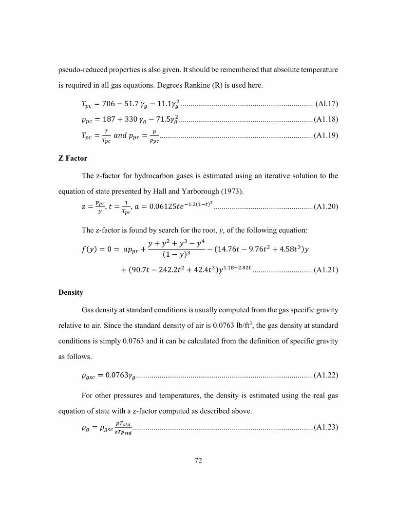
72

pseudo-reduced properties is also given. It should be remembered that absolute temperature

is required in all gas equations. Degrees Rankine (R) is used here.

𝑇𝑝𝑐 = 706 − 51.7 𝛾𝑔 − 11.1𝛾𝑔2 .................................................................... (Al.17)

𝑝𝑝𝑐 = 187 + 330 𝛾𝑔 − 71.5𝛾𝑔2 ..................................................................... (A1.18)

𝑇𝑝𝑟 =𝑇

𝑇𝑝𝑐 𝑎𝑛𝑑 𝑝𝑝𝑟 =

𝑝

𝑝𝑝𝑐 ............................................................................... (A1.19)

Z Factor

The z-factor for hydrocarbon gases is estimated using an iterative solution to the

equation of state presented by Hall and Yarborough (1973).

𝑧 =𝑝𝑝𝑟

𝑦, 𝑡 =

1

𝑇𝑝𝑟, 𝑎 = 0.06125𝑡𝑒−1.2(1−𝑡)2

................................................... (A1.20)

The z-factor is found by search for the root, y, of the following equation:

𝑓(𝑦) = 0 = 𝑎𝑝𝑝𝑟 +𝑦 + 𝑦2 + 𝑦3 − 𝑦4

(1 − 𝑦)3− (14.76𝑡 − 9.76𝑡2 + 4.58𝑡3)𝑦

+ (90.7𝑡 − 242.2𝑡2 + 42.4𝑡3)𝑦1.18+2.82𝑡 ............................... (A1.21)

Density

Gas density at standard conditions is usually computed from the gas specific gravity

relative to air. Since the standard density of air is 0.0763 lb/ft3, the gas density at standard

conditions is simply 0.0763 and it can be calculated from the definition of specific gravity

as follows.

𝜌𝑔𝑠𝑐 = 0.0763𝛾𝑔 ........................................................................................... (A1.22)

For other pressures and temperatures, the density is estimated using the real gas

equation of state with a z-factor computed as described above.

𝜌𝑔 = 𝜌𝑔𝑠𝑐𝑝𝑇𝑠𝑡𝑑

𝒛𝑻𝒑𝒔𝒕𝒅 ............................................................................................. (A1.23)

73


The gas formation volume factor is also calculated from the real gas equation of

state using a z-factor as described above. Using the equation, the ratio of reservoir to

standard volumes for a gas is given by the following equation.

𝐵𝑔 =𝑧 𝑝𝑠𝑡𝑑 𝑇

𝑝 𝑇𝑠𝑡𝑑 ...................................................................................................... (A1.24)

Viscosity

Gas viscosity is rarely measured in the laboratory and is normally estimated from

correlations. In IFM, the Lee et al. (1966) correlation is used. The equations are as follows.

𝐴1 =(9.379 + 0.01607𝑀)𝑇1.5

209.2 + 19.26𝑀 + 𝑇, 𝐴2 = 3.448 +

986.4

𝑇+ 0.01009𝑀

𝐴3 = 2.447 − 0.2224 𝐴2

𝜇𝑔 =𝐴1

10000𝑒

𝐴2𝜌𝑔

𝐴3

........................................................................................... (A1.25)

Heat Capacity

Gambill (1957) presented the following correlation for heat capacity that is used in

IFM.

Cpo = 1684+3.389 T[K]

√γo (

J

kg∙K) =

4.80976+0.003552 T[F]

√ρo[lbm/ft3] (

BTU

lbm∙F) ........................ (A1.26)

74

APPENDIX A2: PARAMETER ESTIMATION

In the previous section the representation and estimation of fluid properties was

presented. Besides fluid properties, many additional parameters are required for modeling

integrated systems. These include heat loss coefficients, as well as equipment

specifications and efficiencies. Unfortunately, many of these properties are rarely

measured directly and must be estimated. Even in the case of equipment specifications,

where manufacturers’ specification sheets may be available, the specifications usually give

minimum performance and maximum limits for new equipment. Since many marginal

fields make use of used or old equipment, de-rating must often be applied to determine the

actual equipment performance. This section provides correlations and recommendations

for estimating many of the parameters required for full system modeling. Fluid properties

are covered in a preceding appendix. It should be noted that when valid manufacturers’

data sheets are available, they should be used as a guideline and when experimental or

measured data is available, it should be used. In many cases values will need to be adjusted

to match observed field performance.

HEAT TRANSFER COEFFICIENTS

In general, heat transfer is modeled using the standard equation for heat flow

following the development in Prats (1986) shown as Equation A2.1, where Q/L is the rate

of heat loss per unit length, Rh is the specific thermal resistance in (BTU/ft2-D-°F)-1, and

T is the temperature difference between the equipment and the environment. Note that in

this equation the loss of heat from the equipment is positive when the equipment

temperature is greater than the environment temperature, so that T is positive. Prats (1986)

75

also provides information on calculating heat losses from insulated pipes and contains

material properties for estimating thermal parameters for a variety of materials.

𝑄 ∆𝐿⁄ = ∆𝑇/𝑅ℎ .............................................................................................. (A2.1)

Following Prats’ development, it is assumed that the pipes consist of internal scale,

metal pipe wall, an external scale coating, and an insulation coating. Outside the pipe

forced convection of air may also be considered for raised pipes or heat loss to the

surrounding soil if the pipe is buried. Note that Prats also includes a laminar film for steam

laden pipes, but that is ignored in this development and it is assumed that liquid coats the

inside of the pipes and is at the fluid temperature. Under those constraints the composite

thermal resistance is given by:

𝑅ℎ =1

2𝜋[

1

ℎ𝑃𝑖𝑟𝑖+

1

𝜆𝑃ln

𝑟𝑜

𝑟𝑖+

1

ℎ𝑃𝑜𝑟𝑜+

1

𝜆𝑖𝑛𝑠ln

𝑟𝑖𝑛𝑠

𝑟𝑜+

1

ℎ𝑓𝑐𝑟𝑖𝑛𝑠] ..................................... (A2.2)

where 𝜆𝑃 and 𝜆𝑖𝑛𝑠 represent the thermal conductivity of the pipe and insulation, hPi and hPo

represent the heat transfer coefficient across the inner and out scale deposits, and hfc

accounts for heat transfer due to forced convection from outside the pipe. Note that heat

radiation is ignored, since the temperature at the outside surface is usually not large. For

most purposes, it can also be assumed that the contact between the inside and outside scale

deposits and the pipe are good, so those respective terms can be ignored, resulting in the

following equation.

𝑅ℎ =1

2𝜋[

1

𝜆𝑃ln

𝑟𝑜

𝑟𝑖+

1

𝜆𝑖𝑛𝑠ln

𝑟𝑖𝑛𝑠

𝑟𝑜+

1

ℎ𝑓𝑐𝑟𝑖𝑛𝑠] ............................................................. (A2.3)

Note that for uninsulated pipe, rins/ro = 1 and the logarithm term becomes zero.

From table B.9 in Prats (1986), the thermal conductivity of carbon steel is about

600 BTU/D-ft-°F and the thermal conductivity of insulation may be in the range of 1 – 10

BTU/D-ft-°F. According to Prats(1986), the heat transfer coefficient for forced convection

due to wind is estimated as:

76

ℎ𝑓𝑐 =18

𝑟𝑒(𝑟𝑒𝑣𝑤)0.6(BTU/D-ft-°F) ....................................................................... (A2.4)

where vw is the wind velocity normal to the pipe in mi/hr and re is the radius exposed to air

in ft.

77

References

Aho, A.V., Hopcroft, J.E. and Ullman, J.D. 1983 Data Structures and Algorithms,

Addison-Wesley Publishing Company.

Arnold, K. and Stewart, M. 1999 Surface Production Operations, Volume 1, Design of

Oil Handling Systems and Facilities, Butterworth-Heinemann.

Bánzer S., C. 1996 Correlaciones Numéricas P. V. T., Maracaibo, Venezuela:

Universidad de Zulia.

Barreto Filho, M. de A. 2001 ‘Estimation of Average Reservoir Pressure and Completion

Skin Factor of Wells that Produce Using Sucker Rod Pumping’, University of

Texas at Austin

Beal, C. 1946 ‘The viscosity of air, water, natural gas, crude oil and its associated gases

at oil field temperatures and pressures’, TP 2018, 94–115

Beggs, H.D. and Robinson, J.R. 1975 ‘Estimating the viscosity of crude oil systems’,

Journal of Petroleum technology 27, 1140–41

Bergant, A., Ross Simpson, A. and Vìtkovsk, J. 2001 ‘Developments in unsteady pipe

flow friction modelling’, Journal of Hydraulic Research 39, 249–57

Bird, R.B., Stewart, W.E. and Lightfoot, E.N. 2007 Transport Phenomena, (Second

Edition, ). New York, NY: John Wiley & Sons, Inc.

Brill, J.P. and Mukherjee, H. 1999 Multiphase Flow in Wells, Vol 17 Richardson, TX:

Monograph Series, SPE.

Chisholm, D. 1967 ‘A theoretical basis for the Lockhart-Martinelli correlation for two-

phase flow’, International Journal of Heat and Mass Transfer 10, 1767–78

Csaszar, A.B., Laine, R.E., Keating, J.F. and Jennings, J.W. 1991 ‘Sucker-Rod Pump

Diagnosis With Fluid Inertia Considerations’, in SPE Production Operations

SymposiumSociety of Petroleum Engineers.

Daugherty, R.L. and Franzini, J.B. 1965 Fluid mechanics with engineering applications, .

New York: McGraw-Hill.

Doty, D.R. and Schmidt, Z. 1983 ‘An improved model for sucker rod pumping’, Soc. Pet.

Eng. AIME, Pap.;(United States) 23,

Earlougher, R.C. 1977 ‘Monograph vol. 5: Advances in Well Test Analysis’, Society of

Petroleum Engineers 90–104

78

Everitt, T.A. and Jennings, J.W. 1992 ‘An improved finite-difference calculation of

downhole dynamometer cards for sucker-rod pumps’, SPE production

engineering 7, 121–27

Frankiewicz, T. and Lee, C.-M. 2002 ‘Using Computational Fluid Dynamics (CFD)

Simulation to Model Fluid Motion in Process Vessels on Fixed and Floating

Platforms’, in SPE Paper 77494. San Antonio, TX.:

Gambill, W.R. 1957 ‘You Can Predict Heat Capacities’, Chemical Engineering 243–48

Gibbs, S.G. 1963 ‘Predicting the Behavior of Sucker-Rod Pumping Systems’, Journal of

Petroleum Technology 15,

Gibbs, S.G. and Neely, A.B. 1966 ‘Computer diagnosis of down-hole conditions in

sucker rod pumping wells’, Journal of petroleum technology 18, 91–98

Govier, G.W. and Aziz, K. 2008 The Flow of Complex Mixtures in Pipes, (2nd Edition, ).

Richardson, TX: Society of Petroleum Engineers.

Gray, H.E. 1963 ‘Kinematics of Oil-Well Pumping Units’, Drilling and Production

Practice

Hafskjols, B., Celius, H.K. and Aamo, O.M. 1999 ‘A New Mathematical Model for

Oil/Water Separation in Pipes and Tanks’, SPE P&F 14, 30–36

Hall, K.R. and Yarborough, L. 1973 ‘A new equation of state for Z-factor calculations’,

Oil and Gas journal 71, 82–92

Hallinger, A., Soenstaboe, F. and Knutsen, T. 1996 ‘A Simulation Model for Three-Phase

Gravity Separators’, in SPE Paper 36644. Denver, CO:

Hilborn, R.C., Coppersmith, S., Mallinckrodt, A.J. and McKay, S. 1994 ‘Chaos and

nonlinear dynamics: an introduction for scientists and engineers’, Computers in

Physics 8, 689–689

Himmelblau, D.M. and Bischoff, K.B. 1968 Process Analysis and Simulation:

Deterministic Systems, . New York, NY: John Wiley & Sons, Inc.

Holman, J.P. 1958 Heat Transfer, (4th Edition, ). New York, NY: McGraw-Hill Book

Co.

IOGCC 2008 Marginal Wells: Fuel for Economic Growth, Interstate Oil and Gas

Compact Commission.

Kolev, N.I. 2002 Multiphase Flow Dynamics 1, Fundamentals, . Berlin: Springer-Verlag.

79

Langston, L.V. 2003. ‘The Lease Pumper’s Handbook, First Edition’

Lee, A., González, M. and Eakin, B. 1966 ‘The viscosity of natural gases’, Journal of

Petroleum Technology 18, 997–1000

Lekia, S.D.L. (Unocal P. and D.T. and Evans, R.D. (Univ of O. 1995 ‘A Coupled Rod

and Fluid Dynamic Model for Predicting the Behavior of Sucker-Rod Pumping

Systems. Part 1: Model Theory and Solution Methodology’, SPE Production and

Facilities (Society of Petroleum Engineers); (United States) 10:1,

Lockhart, R.W. and Martinelli, R.C. 1949 ‘Proposed Correlation of Data for Isothermal

Two-Phase, Two-Component Flow in Pipes’, Chemical Engineering Progress 45,

39–48

McCain Jr, W.D. 1990 The Properties of Petroleum Fluids, Tulsa, OK: PennWell Books.

McCain Jr, W.D. 1991 ‘Reservoir-Fluid Property Correlations—State of the Art’, SPE

Reservoir Engineering

Minami, K. 1991 ‘Transient Flow and Pigging Dynamics in Two-Phase Pipelines’, The

University of Tulsa

Minami, K. and Shoham, O. 1994 ‘Transient two-phase flow behavior in pipelines-

experiment and modeling’, International journal of multiphase flow 20, 739–52

Pennebaker, S. 2014. ‘Personal Communication’

Prats, M. 1986 Thermal Recovery, volume 7 of SPE Monograph Series, Society of

Petroleum Engineers.

RELAP5 2012 RELAP5-3D© Code Manual Volume I: Code Structure, System Models

and Solution Methods, Idaho National Laboratory.

Rosso, F. and Sona, G. 2001 ‘Gravity-driven separation of oil-water dispersions’,

Advances in Mathematical Sciences and Applications 11, 127–51

Rowe Jr, A.M. and Chou, J.C. 1970 ‘Pressure-volume-temperature-concentration relation

of aqueous sodium chloride solutions’, Journal of Chemical and Engineering

Data 15, 61–66

Schafer, D.J. and Jennings, J.W. 1987 ‘An investigation of analytical and numerical

sucker rod pumping mathematical models’, in SPE Annual Technical Conference

and ExhibitionSociety of Petroleum Engineers.

80

Shirdel, M. 2010 ‘Development of a Coupled Wellbore-Reservoir Compositional

Simulator for Horizontal Wells’, MS Thesis, University of Texas

Shirdel, M. 2013 ‘Development of a Coupled Wellbore-Reservoir Compositional

Simulator for Damage Prediction and Remediation’, University of Texas at

Austin

Shoham, O. 2006 Mechanistic Modeling of Gas-Liquid Two-Phase Flow in Pipes, .

Richardson, TX: Society of Petroleum Engineers.

Song, J.H., Jeong, B.E., Kim, H.J. and Gil, S.S. 2010 ‘Three-Phases Separator Sizing

Using Drop Size Distribution’, in OTC Paper 20558. Houston, TX:

Standing, M.B. 1977 Volumetric and Phase Behavior of Oil Filed Hydrocarbon Systems,

. Dallas, TX: SPE of AIME.

Taitel, Y. and Dukler, A.E. 1976 ‘A model for predicting flow regime transitions in

horizontal and near horizontal gas-liquid flow’, AIChE Journal 22, 47–55

Valeev, M.D. and Repin, N.N. 1976 ‘IZVESTIYA VYSSHIKH VCHEBNYKH

ZAVEDENII’, NEFT I GAZ 8, 33–44

Whitson, C.H. and Brulé, M.R. 2000 Phase Behavior, Vol 20 Richardson, TX:

Monograph Series, SPE.

Xu, J., Doty, D.R., Blais, R., Shahraki, A. and Lea, J. 1999 ‘A comprehensive rod-

pumping model and its applications to vertical and deviated wells’, in SPE mid-

continent operations symposium 637–45

Copyright by Walter Benjamin Fair, Jr. 2019

Documents

Transcript of Copyright by Walter Benjamin Fair, Jr. 2019