Copyright by Trevor Scott Ricker 2017
47
Copyright by Trevor Scott Ricker 2017
Transcript of Copyright by Trevor Scott Ricker 2017

Copyright
by
Trevor Scott Ricker
2017

The Thesis Committee for Trevor Ricker
Certifies that this is the approved version of the following thesis:
Position Based Laser Power (PBLP) Control
for Selective Laser Sintering (SLS)
APPROVED BY
SUPERVISING COMMITTEE:
Joseph J. Beaman, Jr.
Scott Fish
Supervisor:

Position Based Laser Power (PBLP) Control
for Selective Laser Sintering (SLS)
by
Trevor Scott Ricker
Thesis
Presented to the Faculty of the Graduate School of
The University of Texas at Austin
in Partial Fulfillment
of the Requirements
for the Degree of
Master of Science in Engineering
The University of Texas at Austin
December 2017

iv
Acknowledgements
I would like to express my gratitude to my advisors, Dr. Beaman and Dr. Fish, for the
opportunity to join their lab and work with the LAMPS machine. Their guidance and insights have
provided structure and focus to my research. I have greatly enjoyed learning about the field of
additive manufacturing and the ongoing research done here at UT.
Additionally, I would like to thank the other members of the UT Additive Manufacturing
Lab, specifically Tim Phillips, Austin McElroy, and Adam Lewis, for their support throughout this
project. Their extensive knowledge of the LAMPS machine and willingness to teach others its
intricacies have made this thesis possible.
I would also like to thank Schlumberger Technology Corporation for providing me with
the opportunity to attend the University of Texas at Austin to receive my M.S. in Mechanical
Engineering. I am fortunate to be able to further my education while continuing my employment
with Schlumberger.

v
Abstract
Position Based Laser Power (PBLP) Control
for Selective Laser Sintering (SLS)
Trevor Scott Ricker, M.S.E.
The University of Texas at Austin, 2017
Supervisor: Joseph J. Beaman, Jr.
This thesis investigates a method for designing, implementing, and testing a Position Based Laser
Power (PBLP) controller for a Selective Laser Sintering (SLS) machine. Current commercial laser
scanning systems do not allow for variable laser power control along the length of a scan line. As
found in previous work, varying the power across a scan line is important to achieving a uniform
post-sintering temperature in the presence of a temperature gradient across the build surface
(Phillips, 2016). By implementing a PBLP control system, the laser power can be varied across
the length of a scan line to correct for variation in pre-sintering temperatures, leading to constant
post-sintering temperatures and improved part quality and consistency.

vi
Table of Contents
Acknowledgements ............................................................................................................ iv
Abstract ............................................................................................................................... v
List of Figures .................................................................................................................. viii
Chapter 1: Introduction ....................................................................................................... 1
1.1: THE SLS PROCESS ................................................................................................ 1
1.2: Experimental Motivation ......................................................................................... 2
Chapter 2: Current LAMPS Laser Scanning System .......................................................... 6
2.1: Overview .................................................................................................................. 6
2.2: Laser Power Control ................................................................................................ 8
2.3: Galvanometer Position Control ................................................................................ 8
2.4: Timing and Delays ................................................................................................. 12
Chapter 3: Design Options ................................................................................................ 14
3.1: Full Rebuild of the laser scanning System ............................................................. 14
3.2: Modified Laser Power Control based on position.................................................. 15
Chapter 4: Final Design .................................................................................................... 17
4.1: Overview ................................................................................................................ 17
4.2: Hardware ................................................................................................................ 18
4.3: Software ................................................................................................................. 20
Chapter 5: Experimental Methods and Results ................................................................. 24

vii
5.1: Laser Power Benchmark Testing ........................................................................... 24
5.2: Mylar Testing ......................................................................................................... 25
5.3: Single Line Test ..................................................................................................... 31
Chapter 6: Conclusion....................................................................................................... 35
References ......................................................................................................................... 37

viii
List of Figures
Figure 1: Selective Laser Sintering Process (Carpenter, 2014) ...................................................... 2
Figure 2: Build Surface Temperature Gradient (Bourell, Watt, Leigh, & Fulcher, 2014) ............. 3
Figure 3: Pre-Sintering And Post-Sintering Temperatures Along A Scan Line (Phillips, 2016) ... 4
Figure 4: Cad Rendering Of The Lamps Machine (Phillips, 2016) ................................................ 6
Figure 5: Current Lamps Laser Scanning System .......................................................................... 7
Figure 6: Micro-Vectoring (Cambridge Technology, 2014) ........................................................ 10
Figure 7: Phase Delay Of The Lamps Galvanometer Response ................................................... 11
Figure 8: Time Delay Of The Lamps Galvanometer Response .................................................... 12
Figure 9: Delays In The Lamps Laser Scanning System .............................................................. 13
Figure 10: Full Rebuild Of Ec1000 Controller ............................................................................. 14
Figure 11: Modified Laser Power Controller ................................................................................ 16
Figure 12: Modified Laser Power Controller ................................................................................ 18
Figure 13: Software Flow Chart ................................................................................................... 20
Figure 14: Power Map Structure ................................................................................................... 22
Figure 15: Example Power Map And Resulting Power Profile .................................................... 22
Figure 16: Power (In Watts) Measured At Various Pwm Periods And Duty Cycles ................... 25
Figure 17: Power Variation Grid .................................................................................................. 26
Figure 18: Power Map .................................................................................................................. 27
Figure 19: 1500 Mm/S With Power Variation From 0%-100% ................................................... 27
Figure 20: 1500 Mm/S With Power Variation From 30%-46% ................................................... 28
Figure 21: Mylar Test 1500 Mm/S ............................................................................................... 29
Figure 22: 750 Mm/S Scans .......................................................................................................... 29

ix
Figure 23: 500 Mm/S Scans .......................................................................................................... 30
Figure 24: 500 Mm/S Power Variation Scan And Power Map .................................................... 31
Figure 25: Single Line Scan With Duty Cycle = 30% .................................................................. 33
Figure 26: Single Line Scan With Duty Cycle = 40% .................................................................. 34
Figure 27: Single Line Scan With Power Variation ..................................................................... 34

1
Chapter 1: Introduction
1.1: THE SLS PROCESS
Selective Laser Sintering (SLS) is a powder fusion based additive manufacturing process
which was developed at the University of Texas at Austin. As the name suggests, a laser is used
to selectively heat portions of a flat powder bed, ‘sintering’ or melting the powder together to
create a desired two-dimensional shape. This shape corresponds to a single cross-section of a three-
dimensional part. By stacking multiple cross-sections together, a three-dimensional part is formed.
In SLS, similar to other additive manufacturing techniques, a 3D model is sliced into two
dimensional layers, which are then sliced into a series of lines, or vectors, which represent laser
scan paths. The process begins with a build chamber which is partially full of powder. This build
chamber is heated to a preset temperature below the melting point of the material being used. Next,
a roller is used to spread a thin, even layer of powder across the top of the build chamber. The laser
is then used to selectively melt a portion of the powder layer corresponding to a 2D cross sectional
area of the final part. The roller then spreads a new layer and the process is repeated for each 2D
cross section until the full three dimensional part is built.

2
Figure 1: Selective Laser Sintering Process (Carpenter, 2014)
1.2: Experimental Motivation
Previous work has shown that the quality of a part built using Selective Laser Sintering is
highly affected by the temperature control of the part during the build (Benda, 1994) (Wroe, et al.,
2016). More specifically, the maximum temperature of each particle of powder during the laser
melting process is critical to achieving a high quality part. If the maximum temperature is too low,
the powder does not fully melt, resulting in a poor bond and a structural weakness. Conversely, if
the maximum temperature is too high, over sintering occurs which can cause part growth and
dimensional inaccuracies. The maximum temperature of the powder is influenced by the pre-
sintering temperature of the powder and the amount of energy deposited by the laser. Theoretically,
the powder bed can be heated to a uniform temperature just below the melting temperature and a
constant laser power can then be used to further heat the powder to the optimal temperature.

3
To achieve this thermally uniform powder bed, SLS machines can have an insulated build
chamber which is heated with a series of radiant heaters. These heaters can be placed strategically
throughout the machine to create a uniform temperature, however geometrical limitations of the
build chamber can limit their effectiveness. A typical commercial machine has a temperature
gradient of 10-15 degrees Celsius across the powder bed (Hall, 2015) (Bourell, Watt, Leigh, &
Fulcher, 2014). Additionally, during a build new variations in temperature across the powder bed
surface can develop due to the presence of previously sintered layers underneath the freshly spread
powder layer (Phillips, 2016).
Figure 2: Build Surface Temperature Gradient (Bourell, Watt, Leigh, & Fulcher, 2014)
Previous work has shown that if a temperature gradient exists in the pre-sintered powder
bed, this gradient will also be reflected in the maximum temperature of the powder during the
sintering process if a constant laser power is used (Phillips, 2016). Figure 3 shows the results of
this work, illustrating that if the pre-sintering temperatures are shifted up by adding a constant to
them, they match the post-sintering temperatures extremely well. This thermal gradient, preserved
in the post-sintering temperatures, will lead to regions of un-melted and over sintered powder,
leading to structural weakness or part deformity as described above.

4
Figure 3: Pre-Sintering and Post-Sintering Temperatures Along a Scan Line (Phillips, 2016)
Since it is difficult to create a fully thermally uniform powder bed, another option is to vary
laser power across the powder bed. By varying laser power inversely with respect to pre-sintered
temperature, the goal of a uniform (and optimal) maximum temperature can be achieved. Previous
work at The University of Austin at Texas has verified that this is a viable solution to the problem
of a temperature gradient (Phillips, 2016). However, limitations in current off-the-shelf laser
scanning systems makes implementation difficult. Current commercial laser scanning systems do
not allow the laser power to be varied across the length of a single scan line. In previous
experiments, a single scan line was divided into multiple smaller scan lines which were each given
a constant power. Although this method is effective in reducing the post-sintering temperature
gradient, dividing a single scan line into multiple smaller scan lines can cause addition problems
with uneven heating of the powder bed. At the beginning and end of each scan line, there is an

5
acceleration region due to the inertia of the galvanometers. If a constant laser power is used during
this acceleration region, more energy is deposited per unit area at the lower velocity, leading to an
increase in temperature of that area. A more complete solution is to continuously vary the power
across the entire scan line, allowing the post-sintering gradient to be reduced without creating
additional hot-spots due to acceleration regions. This paper reviews the design and implementation
of a modified laser scan system which allows the laser power to be varied across a scan line based
on the position of the galvanometers. Although the scan system was only tested for polymer
powders, it should be equally beneficial for SLS of any material.

6
Chapter 2: Current LAMPS Laser Scanning System
2.1: Overview
The LAMPS (Laser Additive Manufacturing Pilot System) machine is an SLS machine
that was designed and built at the University of Texas at Austin. Full details of the LAMPS
machine can be found in other papers (Wroe, Improvements and Effects of Thermal History on
Mechanical Properties for Polymer Selective Laser Sintering (SLS), 2015); this section will focus
on the laser scanning system as this is the only portion of the machine that was modified.
Figure 4: CAD Rendering of the LAMPS Machine (Phillips, 2016)
The current LAMPS laser scanning system is a two axis galvanometer system coupled with
a 40 watt CO2 laser. The galvanometer (galvanometer) system is made by Cambridge Technology
and includes a self-contained controller called the EC1000, a digital to analog converter, two

7
MiniSAX servo controllers (one for each axis of motion), and the galvanometers themselves. The
CO2 laser is the 40 watt CO2 laser from the Infinity Series made produced by Iradion. A flow chart
of the inputs and outputs to each component of the laser scanning system is shown below in Figure
5.
Figure 5: Current LAMPS Laser Scanning System
The EC1000 receives commands from the LAMPS host computer via an Ethernet cable
and then controls the laser power and scanning position according to these commands. There are
two main EC1000 commands used in LAMPS: the mark command and the jump command. The
mark command moves the galvanometer’s to the specified position with the laser on; the jump
command moves the galvanometer’s with the laser off. Both commands are only end point
commands- the EC1000 will move the galvanometers to the specified position from wherever its
current position is. For example, a jump command of JUMP (20,30) moves the galvanometers so
that the laser spot is focused on the point X = 20 mm and Y = 30 mm from the center of the build
chamber. The build area is 200 mm by 200 mm, with positions on the build surface varying from
(X, Y) = (-100, -100) to (X,Y) = (100, 100).

8
2.2: Laser Power Control
Laser power is controlled by the EC1000 through a digital pulse width modulated signal.
The PWM laser power signal’s period can be modified by the user; it is typically set at 200 μs.
The laser power is specified by the duty cycle and can be changed before each mark command is
issued. This limitation of the current laser scanning system of one laser power per mark command
is the main motivation for developing a new laser scanning system. Note that actual power output
from the laser is not linear with the respect to duty cycle. For example, a specified power of 25%
in the build file corresponds to the EC1000 outputting 50 μs of digital high followed by 150 μs of
digital low, repeated for the duration that the laser is on. Thus, this 25% command represents a
25% duty cycle, however the actual power output from the laser will not necessarily be 25% of the
maximum power of the laser.
When the laser is not in use, a tickle signal is sent to the laser from the EC1000. This is a
low duty cycle PWM, approximately 0.5%-1.5%. The purpose of the tickle is essentially to prime
the laser, thus enabling the timing of the laser turning on to be more accurate.
2.3: Galvanometer Position Control
Galvanometer (galvanometer) position is controlled by the EC1000 by outputting a digital
signal using the XY2-100 protocol. XY2-100 is a protocol for communicating galvanometer
positions which involves three 16 bit position words and a 16 bit status word. Each position word
corresponds to an axis (X, Y, and Z); in the LAMPS 2-axis laser scanning system the Z word is
unused. More details on the XY2-100 protocol can be found in other literature (Shannon &
Weaver, 2008).

9
The XY2-100 signal then passes into a digital/analog converter which output two separate
analog voltages: one for each axis. Each axis then has an independent galvanometer controller
which moves the galvanometer servo motors according to this input voltage, which will be called
the command signal for the remainder of this document. The galvanometer controllers used on the
LAMPS machine are the MiniSAX servo controller by General Scanning Inc. The command signal
is a +/- 3V single ended analog signal. The command voltage corresponds directly to a servo
angular position, which corresponds to a (X,Y) position on the LAMPS powder bed. The transform
from command voltage to powder bed position was found to be linear. Additional details for the
MiniSAX controller can be found in the reference manual (General Scanning Industries, 2006).
The speed at which the galvanometer’s move from one position to the next is controlled
through a process called micro-vectoring. When the EC1000 receives a command to move the
galvanometer’s to a position, it does not simply output a XY2-100 signal with this desired end
position. Instead, it divides this vector into multiple shorter vectors of length dx and updates the
command signal at a constant frequency of 100 kHz. By controlling the length dx, the scanning
speed can be controlled. This leads to a stair shaped command signal, however the galvanometer
response remains smooth due to the servo motor controller. The diagram below in Figure 6 shows
the micro-vectoring process and galvanometer response while moving between positions X0, X1,
X2… etc (Cambridge Technology, 2014).

10
Figure 6: Micro-Vectoring (Cambridge Technology, 2014)
The MiniSAX galvanometer controller also allows for the position of the galvanometer to
be measured while the laser scanning system is operating. The position is measured through
capacitance feedback and is in the form of a +/- 3V differential analog signal. Similar to the
command signal, the position signal can be directly mapped from voltage to position through a
linear transform. For the Y galvanometer, the bias is approximately 0.065 V and the gain is
approximately 77.7 mm/V; for the X galvanometer the, bias is approximately 0.068 V and the gain
is approximately 79.7 mm/V. In the current laser scanning system, this signal is only used
internally to control the galvanometer motion. It is also vital for implementing a position based
laser power control system.
It can also be observed that there is a delay between the command signal and the actual
position of the galvanometer’s. This was characterized experimentally by applying a sinusoidal
input voltage to the galvanometer controller and measuring the position response. This was done
at frequencies varying from 1 Hz to 500 Hz. The resulting frequency response, including both
phase delay and time delay, for both axis are shown below. It is interesting to note the difference
between the X and Y response; both axes have a fairly constant delay of approximately 1.2 ms at

11
lower frequencies, however the delay in the X axis is slightly larger. This may be due to the
different sized mirrors and thus different inertia’s of the two galvanometers. It may also be due to
the geometry of the galvanometer head: one mirror is positioned slightly farther from the build
surface and thus the transform from rotational velocity of the galvanometer to linear velocity on
the build surface is slightly different.
Figure 7: Phase Delay of the LAMPS Galvanometer Response

12
Figure 8: Time Delay of the LAMPS Galvanometer Response
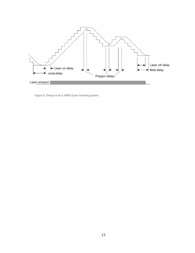
2.4: Timing and Delays
The timing between the galvanometer motion and the laser is controlled by adjusting the
laser on delay and laser off delay. The laser on delay is the time between the first xy2-100 position
command being sent to the galvanometer’s and the laser turning on. The laser off delay is the time
between the last xy2-100 position command being sent to the galvanometer’s and the laser turning
off. These delays are adjustable to account for the delay between command signal and actual
position of the galvanometer’s discussed above, which can vary from system to system based on
a number of variables such as galvanometer inertia, galvanometer controller tuning, and D/A
conversion. The Jump Delay, Mark Delay, and Polygon Delay allow for additional delays to be
added at the end of a jump command, the end of a mark command, or between two successive
mark commands, respectively (Cambridge Technology, 2014).
13
Figure 9: Delays in the LAMPS Laser Scanning System

14
Chapter 3: Design Options
3.1: Full Rebuild of the laser scanning System
The first option to improve the laser power control on the LAMPS machine involves a full
rebuild of the laser scanning controller. Basically, this option involves developing a personalized
EC1000 with all its features tailored to the needs of the LAMPS machine. All the current functions
of the EC1000 would need to be mimicked, along with an additional feature where the power can
be changed along the length of a vector based on position.
Figure 10: Full Rebuild of EC1000 Controller
The main benefits to a full rebuild is flexibility and customizability. Since the new
controller will be built from the ground up, it can be designed to meet all the needs for testing and
experimentation with the LAMPS machine. The controller would be fully customizable and build
to perform as desired. Additionally, if future work requires further modifications of this controller,
these modifications could be implemented at that later date.

15
Disadvantages to the full rebuild are time and cost. A proper rebuild would take a
significant amount of time. The details about how the EC1000 functions must be understood,
limitations and places to improve on the current system must be identified, and new algorithms
would need to be developed to implement the position based laser power. There would need to be
a large amount of testing with the new controller to verify its accuracy and capabilities. All of this
work would delay the implementation of an improved laser power control. Additionally, cost of a
new controller would be in the range of $5000-$10,000, meaning the appropriate budget must be
in place to fund this rebuild.
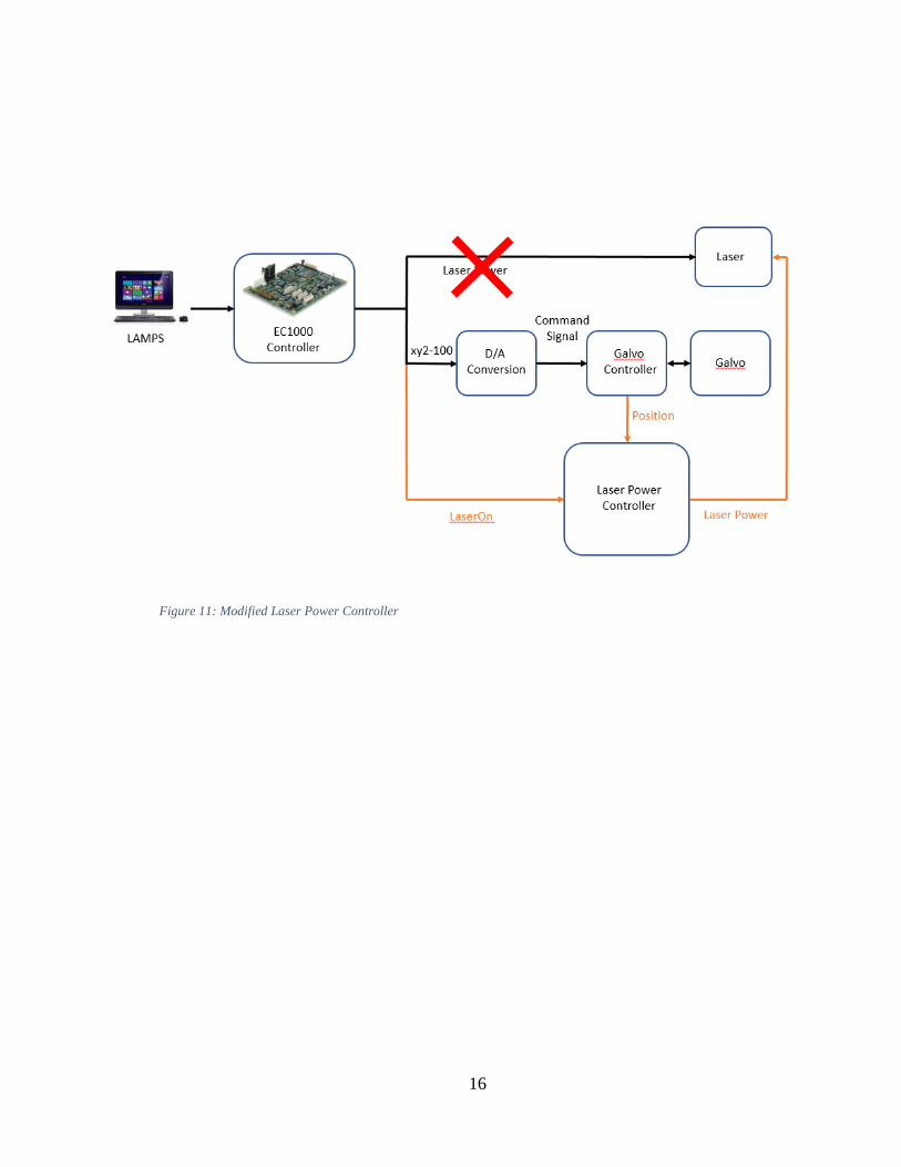
3.2: Modified Laser Power Control based on position
A second option to improve the laser power control involves continuing to use the EC1000
to control the laser scanning while adding a separate controller to implement a position based laser
power (PBLP). This laser power controller would have three inputs: (1) X galvanometer position
from the X miniSAX (2) Y galvanometer position from the Y miniSAX (3) laser on/off from the
EC1000. The controller would output a digital PWM signal to the CO2 laser, similar to the original
EC1000 PWM signal except that the duty cycle could be updated continuously rather than just
once a scan line.
The benefits of adding a PBLP controller are simplicity, time, and cost. This option only
modifies how the laser power signal is generated and leaves the remainder of the current laser
scanning system in place. In this way, it is a much simpler solution than a full rebuild, as only the
parts of the laser scanning system that must be modified are modified. Since the EC1000 will not
need to be redesigned, the implementation time would be significantly reduced. Cost would also
be an order of magnitude smaller than a full redesign.
16
Figure 11: Modified Laser Power Controller

17
Chapter 4: Final Design
4.1: Overview
The decision to implement a Position Based Laser Power (PBLP) controller was made
based on the advantages of decreased time till operational and reduced cost. Also, if in the future
a full redesign of the EC1000 is necessary, the knowledge and solutions implemented in the PBLP
controller can be utilized in this design.
The PBLP controller was developed through the use of two cRIO modules: An analog input
module (NI 9205) and a high speed digital input/output module (NI 9402). The analog input
module is used to read the X and Y galvanometer positions while the digital I/O module is used to
read the LaserOn signal and create the PWM laser power signal. The LaserOn signal is needed as
an input to allow the controller to differentiate between mark commands (movement with the laser
on) and jump commands (movement with the laser off). A flow chart of the new laser scanning
system is shown in Figure 12.
The LaserOn signal is a digital output from the EC1000 which corresponds to the state of
the command being sent from the EC1000 to the CO2 laser. When LaserOn is low, the EC1000
sends the tickle signal to the laser; when LaserOn is high, the EC1000 would be powering the laser
according to the constant power specified in the build configuration. Thus, the LaserOn signal is
used by the PBLP controller as a method to specify when to turn on the laser at the beginning of a
scan line and turn it off at the end of the scan line. Timing of the LaserOn signal with respect to
galvanometer motion is controller through the laser on delay and laser off delay, which were
described in detail above in the ‘Current LAMPS laser scanning system’ section.

18
Figure 12: Modified Laser Power Controller
4.2: Hardware
NI 9402
The National Instruments cRIO module 9402 is a high speed digital input/output module.
The module uses a low volt TTL (LVTTL) signal, meaning the digital high is approximately 3.3
V, which is the same as the output from the EC1000 in the previous system. It has four channels
which can all be individually configured as inputs or outputs; channel 0 is used to create the PWM
output and channel 1 is used to read LaserOn. The module has a BNC interface and a 55 ns
maximum update rate; in its current configuration the LaserOn signal is updated every 150 ns and
the laser power signal can be updated every 250 ns. This update rate allows the duty cycle of the
laser PWM signal to be controlled with a resolution of 0.5% (National Instruments, 2017).

19
NI 9205
The National Instruments cRIO module 9405 is an Analog input module with a push-in
spring terminal interface. The module can measure up to 32 single-ended channels or 16
differential signals (the galvanometer positions are differential signals). Channel 0 is used to
measure Y galvanometer position and channel 1 is used to measure X galvanometer position. The
module is configured to read a +/- 5 V range which gives a resolution of 0.076 mV. The module
has a 4 μs update rate, however simultaneous channel updates are not possible. This means that
when multiple channels, the signals are read in series at the maximum update rate, increases the
effective update time for each channel by multiplying the maximum update rate by the number of
channels currently being updated. This means the effective update rate when reading both X and
Y galvanometer position is 8 μs (National Instuments, 2017).
The position signal read by the NI 9205 module is a direct output from the MiniSAX
galvanometer controllers. The position signal is generated by the MiniSAX galvanometer
controller through capacitance feedback and is a +/- 3V differential, analog, voltage signal. The
voltage corresponds directly to an angular position of the galvanometer, which corresponds to a
mm position on the powder bed surface. Through measurement and experimentation, it was found
that the voltage varies linearly with position. Thus a simple gain and bias can be applied to the
measured X and Y voltage signals to convert them to their corresponding positions. The bias and
gain is calibrated each time the LAMPS machine is run to account for any electric drift that may
be present in the system.

20
4.3: Software
The program was developed in LabVIEW as this is the platform used to run the LAMPS
machine. The program is deployed and executed on the cRIO FPGA due to the high speeds and
consistent timing needed for position based power control. The program is broken down into 3
main sections: data acquisition and filtering, laser power calculation, and PWM implementation.
Additionally, a power map must be separately developed and input to the FPGA program. A flow
chart of the software for the PBLP controller is shown below in Figure 13.
Figure 13: Software Flow Chart
The Power Map
The power map is a two dimensional, user created, power profile which is input to the
FPGA program. This power map governs how the program will control the laser power as the

21
galvanometer position changes. The power map is essentially a two dimensional look up table
which specifies desired powers at user-determined points across the build surface.
The power map is created by specifying an X-position and Y-position array, both of length
14, as well as a single 2D power array of size 14x14. The size of the arrays was limited to 14 by
the space on the cRIO FPGA. The power map is illustrated in Figure 14 below; the user specifies
The X positions (X1-X14), the Y positions (Y1-Y14), and the powers (Power1,1-Power14,14). Each
position array is used to choose 14 points along each axis where the power will be specified
through the power array. The positions have units of mm and must be in descending order. The
power has units of duty cycle percentage and have a resolution of 0.5%. Through this method, the
power can be defined in a 14x14 grid across the build surface. The program will also bilinearly
interpolate between the four closest points, thus allowing an arbitrary power profile to be
developed. The user can choose the positions in any spacing and does not have to use all 14
positions in either axis if it is not desired. An example power map is shown in Figure 15 below;
in this example, two positions in both the X and Y direction are specified to create a power map
which linearly varies the laser power across the entire build surface. The power map can be updated
each layer of the build or multiple times throughout each layer. This allows a very precise power
map to be created to match the needs of the user.

22
Figure 14: Power Map Structure
Figure 15: Example Power Map and Resulting Power Profile
Data Acquisition and Filtering
The digital LaserOn signal is updated at a rate of 150 ns while the analog position signals
are updated at a rate of 8 μs. However, the raw position voltage signal from the galvanometer
controllers contains a large amount of noise: ~2 mV peak to peak which corresponds to

23
approximately 150 μm. This accuracy is not sufficient to implement the desired laser power
control. A 2nd order butterworth filter is used with a sampling frequency of 200kHz and a cutoff
frequency of 1000 Hz. This reduces the noise by an order of magnitude to approximately 0.2 mV
peak to peak, corresponding to 15 μm accuracy. Since the sampling rate is 8 μs, which corresponds
to 12 μm at a scan rate of 1500 mm/s, the post-filtering noise in the position signal is on the same
order of magnitude as the inaccuracies due to latency in the position updates.
Duty Cycle Calculation and PWM Implementation
The duty cycle is calculated by comparing the measured position of both the X and Y
galvanometers to the positions specified in the power map. Bilinear interpolation is performed in
both the X and Y directions to achieve the position based duty cycle. This duty cycle calculation
takes approximately 1.5 μs: thus the total time from reading of a galvanometer position to duty
cycle implementation is less than 10 μs. This is five times faster than duty cycle period of 50 μs,
meaning positional accuracy will not be lost due to compounding of latencies.
The PWM implementation logic is based on the state of the LaserOn signal. If LaserOn is
low, the tickle pulse is implemented; if LaserOn is high, the calculated duty cycle based on position
is implemented. The PWM period can be varied if desired, however all tests used a 50 μs period.

24
Chapter 5: Experimental Methods and Results
5.1: Laser Power Benchmark Testing
The first step in verifying the effectiveness of the PBLP controller was to experimentally
confirm that it could replicate the EC1000’s laser power control. To accomplish this, a power
meter was used to measure the output power from the laser with the duty cycle constant and the
galvanometers in a stationary position. A baseline was recorded with the EC1000 controlling the
laser power and compared to results from the PBLP controller at the same duty cycles. Duty cycles
of 7%, 8%, 25%, 50%, 75%, and 100% were used. It was found that the powers for both controllers
were very similar, confirming that the PBLP controller was able to effectively command the laser.
Additionally, powers were recorded using the PBLP controller and a shortened PWM
period of 50 μs (both of the previous measurements were taken with a 200 μs period). The
shortened period is significant because it determines how often the duty cycle can be updated, and
thus determines the resolution of the laser power controller. At a scan speed of 1000 mm/s, a period
of 200 μs means the power is updated once every 200 μm while a period of 50 μs means the power
is updated every 50 μm. This faster update rate would be very advantageous if it is desirable to
control power at a very small scale. It was found that the shortened PWM period lead to a dramatic
decrease in power at low duty cycles, however the power was relatively unaffected at higher duty
cycles which are typical during a SLS build. The results of these power meter tests are shown in
the in Figure 16 below.

25
Figure 16: Power (in watts) Measured at Various PWM Periods and Duty Cycles
5.2: Mylar Testing
Testing of the PBLP controller using mylar sheets was performed to determine how
effectively the laser power could be varied based on position. Mylar sheets were used for this test
because they provide a convenient way to view the dimensional accuracy of the laser scanning
commands. The mylar sheets are initially black but become white when exposed to a strong,
concentrated energy source, I.E. a laser. This allows a laser scan pattern to be executed and
examined afterward. By varying the laser power during the scan and observing the results on the
mylar, the accuracy of the system was quantified.
Determination of optimal duty cycle
To perform the mylar tests with accurate results, the optimal power to use while scanning
must first be determined. Too high of a laser power creates thicker, less accurate lines on the mylar,
while too low of a laser power does not create a line. To determine this power, a power map was
created that varied the duty cycle linearly across both the X and Y axes. The duty cycle was
specified at 4 points on the powder surface: (20,20) = 100%, (20,-20) = 50%, (-20,20) = 50%, and

26
(-20,-20) = 0%. A scan pattern was created with vertical lines, horizontal lines, and diagonal lines,
all placed 5 mm apart. The scan pattern is shown below in Figure 17, with the resulting power
map shown in Figure 18 with the power being represented through the color of the image. This
scan pattern was used because it allowed for a non-quantitative test of the laser power controller
and allowed for an accurate determination of the optimal duty cycle. The diagonals with a negative
slope (the lines drawn in red) were particularly useful for determining optimal power as these lines
were of constant duty cycle. Scan speeds of 1500 mm/s, 1000 mm/s, 750 mm/s, and 500 mm/s
were used. After the initial test, a subset of the full 0%-100% range was used to more easily and
accurately identify the optimal power. The results show that the optimal duty cycles at scan speeds
of 1500 mm/s, 750 mm/s, and 500 mm/s are 38%, 31%, and 25%, respectively.
Figure 17: Power Variation Grid

27
Figure 18: Power Map
Figure 19: 1500 mm/s with power variation from 0%-100%

28
Figure 20: 1500 mm/s with power variation from 30%-46%
Laser on/off test
The goal of this test was to quantify how accurately the laser power can be modified during
a scan line. This was done by setting the power map so that for all X, when Y > 0, the power is the
optimal writing power, and when Y < 0, the power is 0. The Y = 0 and X=0 lines were scanned at
the optimal power to use as a reference. With this power map, the laser should change state at Y=0,
turning on if scanning in the direction of increasing Y and vice versa. A series of lines were then
scanned with a constant X position and the accuracy of the end of the line with respect to the Y=0
position was observed. Lines scanned from top to bottom (Y=20 to Y=-20) started with the laser
on and turned the laser off at Y=0, while lines scanned from bottom to top (Y=-20 to Y=20) started
with the laser off and turned the laser on at Y=0. Lines were scanned at three speeds (1500, 750,
and 500) and the results are shown below.

29
Figure 21: Mylar Test 1500 mm/s
Figure 22: 750 mm/s Scans

30
Figure 23: 500 mm/s Scans
These results show that the laser is turning off very close to the desired position. This
confirms that the PBLP controller is (1) accurately measuring the position of the galvanometers
and (2) can compute and implement the desired duty cycle based on this position fast enough to
not lose positional accuracy. However, the scan lines where the laser is turning on in the middle
of the scan show a noticeable error between the desired position for the laser to turn on of Y=0 and
the actual position the laser turns on. The measured error is approximately 0.25 mm, 0.4 mm, and
0.90 mm for scan speeds of 500 mm/s, 750 mm/s, and 1000 mm/s, respectively. It is hypothesized
that this error is not a result of the PBLP controller; rather it is due to rise time inherent in the CO2
laser itself. This hypothesis was supported by performing an additional test where the power
variation was reduced: for a scan speed of 1500 mm/s, instead of a step change in power from 0%
to 40% duty cycle, the step change was reduced to 25% to 40%. Similarily, for 750 mm/s scans
the power was varied from 24% to 31% and for 500 mm/s scans the power was varied from 20%
to 25%. If the error was due to latency in the laser rise time, this latency should be reduced since
the change in laser power is reduced. In Figure 22 and Figure 23, the image on the left shows the
power variation from 0% while the image on the right shows the reduced power variation. The
results show that the error decreases significantly when the change in duty cycle is reduced,

31
confirming the hypothesis that error is due to laser power rise time. Typical usage of the PBLP
controller during a build should not involve step changes in power, therefore this issue should not
cause problems during SLS builds.
Additional mylar tests were completed by applying a variable power map and scanning in
the power variation grid pattern discussed above. This allowed for a more comprehensive test of
the PBLP controller than scan lines in the Y direction. Figure 24 below shows the results of one
of these tests, along with the corresponding power profile. The result shows that the PBLP
controller is capable of varying power in all directions effectively, especially at the scan speed of
500 mm/s.
Figure 24: 500 mm/s Power Variation Scan and Power Map
5.3: Single Line Test
The goal of this test was to reduce the post-sintering thermal gradient across a single scan
line through position based power variation. This is a full proof-of-concept test and would verify

32
that the use of the new laser power controller could lead to a more uniform maximum sintering
temperature.
The Boresight Camera
The LAMPS machine is equipped with a “boresight camera”, which is a camera aligned
with the beam of the laser before the galvanometer system. This alignment allows the camera to
follow the path of the laser as it moves across the build surface. The boresight camera is a FLIR
SC8240 which is a high speed mid wave infrared camera capable of recording images with a
resolution of 64x64 pixels at a rate of 2243 Hz.
Experimental Method
A temperature gradient of 10 degrees Celsius was purposefully created across the build
surface for the purpose of this test by modifying the temperature set points of multiple heaters in
the LAMPS build chamber. A single scan line was then scanned three times: once at 30% duty
cycle, once at 40%, and once varying linearly from 40% to 30%. During each scan, the boresight
camera was used to record temperature data in-situ. The temperature of the pixel tracking the center
of the laser, where the temperature was greatest, was then extracted from the recorded images and
plotted over time. In addition, before each scan with the laser on, a pre-scan was completed with
the laser power off to verify the initial temperature gradient. During each pre-scan, the boresight
camera recorded temperature data and the temperature of the same pixel in the image was plotted
over time.
Results
The results of the three scans are shown in Figures 25-27. As expected, the scans completed
with a constant power preserve the initial temperature gradient. However, when the laser power is
varied across the scan line inversely with respect to the pre-sintering temperature gradient, the

33
gradient is eliminated. The scan with varied laser power closely matches the 40% constant power
scan initially, and closely matches the 30% constant power at the end, as expected. The large spike
at the beginning of the scan line is the hot spot formed by the laser being turned on during the
acceleration region of the galvanometers. These tests were focused solely on reducing the
temperature gradient: with proper tuning of the laser on/laser off delays the hot spot would be
reduced significantly. The variance in the post-sintering temperature is repeatable for the same
positions; this repeatability may be due to uneven transmittance of laser power through the window
due to buildup from previous builds.
Figure 25: Single Line Scan with Duty Cycle = 30%

34
Figure 26: Single Line Scan with Duty Cycle = 40%
Figure 27: Single Line Scan with Power Variation
35
Chapter 6: Conclusion
This thesis presents a method for designing, implementing, and testing a Position Based
Laser Power (PBLP) controller for a Selective Laser Sintering machine. A commercial laser
scanning system was modified to allow for position based power control of a commercial CO2
laser. A cRIO microcontroller was used as the platform to implement this modified laser power
control, while the previous galvanometer control system was left in place. This solution allowed
for a working system to be implemented with minimal cost and time.
The resulting PBLP controller has a 50 μs update rate with a position resolution of 10 μm
and a power resolution of 0.5% duty cycle. The power map used to determine the output laser
power based on position allows for 14 points in both the X and Y direction to be chosen arbitrarily
and an individual power assigned to each of these 196 points. The power is bilinearly interpolated
between points, leading to a smooth two-dimensional power profile which can be customized to
meet the user’s needs. The software was implemented on the cRIO FPGA to meet the strict timing
needs of the laser scanning system.
The results of the mylar testing show that the PBLP controller can accurately modulate the
power across a single scan line. It was found that the latency intrinsic to the CO2 laser was the
limiting factor when determining the positional accuracy. The results of the single scan line test
using the high-speed infrared camera show that by varying the power across a scan line, a
temperature gradient in the pre-sintered powder can be compensated for to achieve a uniform post-
sintering temperature.
Future work using the PBLP controller can expand on these experiments by implementing
PBLP control in a full SLS build. To accomplish this, power maps will need to be generated in

36
real-time based on the temperature profile of the build surface. Another area for future work would
be to research CO2 laser dynamics and determine how the latency in the current laser could be
reduced. A full redesign of the EC1000 controller would be beneficial by allowing for more
flexibility in the control of the motion of the galvanometer system. The current system only allows
for a constant velocity to be specified between two points with no control of galvanometer
acceleration. By designing and building a custom EC1000-like controller, acceleration could be
controlled, allowing for a more exact motion profile to be specified.

37
References
Benda, J. A. (1994). Temperature-Controlled Selective Laser Sintering. Solid Freeform
Fabrication Symposium. Austin.
Bourell, D. L., Watt, T. J., Leigh, D. K., & Fulcher, B. (2014). Performance Limitations in Polymer
Laser Sintering. Physics Procedia, 147-156.
Cambridge Technology. (2013). EC1000: Hardware Reference Manual. USA: Cambridge
Technology, Inc.
Cambridge Technology. (2014). EC1000: Software Reference Manual. USA: Cambridge
Technology, Inc.
Carpenter, D. (2014). Robotics Projects at NAIT. Retrieved from http://www.acamp.ca/.
General Scanning Industries. (2006). MiniSAX: User's Manual. Retrieved from
http://files.engineering.com/download.aspx?folder=bf43f662-cfd3-48a5-b76f-
8d50510d8052&file=176-25016_MiniSAX_Manual_G.pdf
Hall, P. (2015). SLS Process Overview. (T. Phillips, Interviewer)
National Instruments. (2017). NI 9402: Datasheet. Retrieved from
http://www.ni.com/pdf/manuals/374614a_02.pdf
National Instuments. (2017). NI 9205: Datasheet. Retrieved from
http://www.ni.com/pdf/manuals/378020a_02.pdf
Phillips, T. (2016). In-Situ Laser Control Method for Selective Laser Sintering. Austin: University
of Texas, Austin.

38
Shannon, M., & Weaver, C. (2008). XY2-100 Serial Link 1 Specification. GSI Group Inc.
Wroe, W. W. (2015). Improvements and Effects of Thermal History on Mechanical Properties for
Polymer Selective Laser Sintering (SLS). Austin: University of Texas, Austin.
Wroe, W. W., Gladstone, J., Phillips, T., Fish, S., McElroy, A., & Beaman, J. (2016). In-situ
thermal image correlation with mechanical properties of nylon-12 in SLS. Rapid
Prototyping Journal, Vol. 22 Iss. 5, 794-800.