Copyright by German A. Monroy 2005nn.cs.utexas.edu/downloads/papers/monroy.thesis05.pdf · by...

Copyright

by

German A. Monroy

2005

Coevolution of Neural Networks Using a Layered Pareto Archive

by

German A. Monroy, B.S.

Thesis

Presented to the Faculty of the Graduate School

of The University of Texas at Austin

in Partial Fulfillment

of the Requirements

for the Degree of

Master of Arts

The University of Texas at Austin

August 2005


APPROVED BY

SUPERVISING COMMITTEE:

_____________________________ Risto Miikkulainen

_____________________________ Bruce Porter

Dedicated to my father, mother, sister and brother

v

ACKNOWLEDGEMENTS

I would like to thank Risto Miikkulainen for his optimistic and patient support during all stages of

this thesis. With his generous advice he allowed me to fulfill the dream of being introduced to the

worldwide research community. I would also like to thank Ken Stanley, for his constant

enthusiasm, his willingness to discuss the details of this project and the confidence that he

instilled in me. I would like to acknowledge the help of Vishal Arora, when this thesis began as

class project that he embraced. Thanks for those challenging discussions and for introducing me

to Eclipse. Thanks to Ugo Vieruchi for coding JNeat, which I used as the base to write the

simulations. I want to express my appreciation to the Neural Networks group, for their excitement

to understand and contribute to this project. Special thanks to Uli Grasemann, Lisa

Kaczmarczyk, Nate Kohl, Judah De Paula, Tal Tversky and Jeff Provost for their valuable insights

and for their coaching with presentations, research and even ergonomics. I want to thank all of

my friends for their encouragement and the help that they gave me at different moments during

the making of this thesis: Maria Clara Afanador, Heather Alden, Ricardo Alonso, Emérita Benitez,

Claudia Bustamante, Pablo Carrillo, Natalia Carrillo Bustamante, Huáscar García, Jan

Fernheimer, Maceci Forero, Natalia Gómez, David González, Juan Carlos Hidalgo, Jeff Hoelle,

Erick Leuro, Camila Montoya, José Fernando Orduz, Leonardo Ramirez, Esteban Ribero, Lina

Rueda, Martha Sáenz, Anne Schluter, Julián Sosa, David Suescún, Sonia Uribe and Malathi

Velamuri.

I will always be grateful to the instructors who led me through the masters program: Gordon

Novak, Lorenzo Alvisi, Hamilton Richards, Vladimir Lifschitz, Bruce Porter, Jayadev Misra,

Shyamal Mitra, Risto Miikkulainen and Anna Gal in Computer Sciences and David Hall, Tom

Juenger and Sarah Joseph in Biology. I can not thank enough the enormous support I received

from Gloria Ramirez, Katherine Utz, Bruce Porter, Shyamal Mitra and Roger Priebe. I treasure

the opportunity and responsibility I was given to be a Teaching Assistant. I also want to thank the

staff of the CS department for a perfectly ran infrastructure. I am fortunate to have had as fellow

students Nalini Belaramani, Onur Buk, Doo Soon Kim, Dmitry Kit, Prateek Gupta, Brandon Hall,

Susan Overstreet, Jenniffer Sartor, Subramaniam Venkiteswaran and Matt Walker. I came here

in the first place with the help of David Hite, Javier Villamizar and José Fernando Vega. Thank

you so much for believing in me. I also want to express thanks to Colfuturo for giving me the

financial opportunity to undertake this masters and to the Universidad Javeriana for my academic

foundations as well as for the chance to be one of their instructors.

vi

I want to give special thanks to Stacy Miller and Phillip Keil for being so kind and for some of the

best moments I spent in Austin. My experience in Texas would not have been complete without

having met Lindsey and Annie Rush, Arika Kulhavy and Louise Donnell; thank you and your

families for receiving me in your homes. Big thanks to the rest of my friends who made it such a

pleasure to live in Austin: Martha Bernal, René and Maria Brito, Catalina Estrada, Luis Fujiwara,

Andrés Manosalva, Filadelfo Martínez, Michael O’Brien, Katie Rush, Jenny Achilles, Miguel

Rodríguez, Paula San Martin and Michelle Zisson. And also to those who made me feel their

presence in spite of the distance: the Baez Vásquez family (Elsa, Jorge, Sara and Ana Sofia),

Patty Coronado, Alejandro González, Jairo Hurtado, my uncle Angel Rafael Monroy, Jorge

Iñiguez, the Orduz Sánchez Family, Jaime Peña, Mónica Rincón, the Rojas González family,

Claudia Sánchez and last but not least, the rest of my family: aunts, uncles, cousins and

grandmother.

This research was supported in part by the National Science Foundation under CISE Research

Infrastructure Grant EIA-0303609.

vii


by

German A. Monroy, M.A.

The University of Texas at Austin, 2005

SUPERVISOR: Risto Miikkulainen

Evolutionary computation (EC) can be used to discover good game playing strategies with

respect to a fixed group of existing opponents. Competitive coevolution (CC) is a generalization

of EC in which the opponents also evolve, making it possible to find strategies for games in which

no good players already exist. Since the performance criterion in CC changes over generations,

a Coevolutionary Memory (CM) of good opponents is required to avoid regress. The Layered

Pareto Coevolution Archive (LAPCA) was recently proposed as an effective CM that guarantees

monotonic progress under certain assumptions. The main limitation of LAPCA is that it requires

numerous game evaluations because it has to determine Pareto-dominance relations between

players. The Hall of Fame (HOF), consisting of previous generation champions, is an easier CM

to implement and needs no extra evaluations besides those required by evolution. While the

LAPCA has only been demonstrated in artificial numeric games, the HOF has been applied to

real world problems such as the coevolution of neural networks.

This thesis makes three main contributions. First, a technique is developed that interfaces the

LAPCA algorithm with NeuroEvolution of Augmenting Topologies (NEAT), which has been shown

to be an efficient method of neuroevolution in game playing domains. The technique is shown to

keep the total number of evaluations in the order of those required by NEAT, making it applicable

to practical domains. Second, the behavior of LAPCA is analyzed for the first time in a complex

game playing domain: evolving neural network players for the game of Pong. Third, although

LAPCA and HOF perform equally well in this domain, LAPCA is shown to require significantly

less space than the HOF. Therefore, combining NEAT and LAPCA is found to be an effective

approach to coevolution; the main task for the future is to test it in domains that are more

susceptible to forgetting than Pong, where it can potentially lead to improved performance as

well.

viii

TABLE OF CONTENTS

1. Introduction .................................................................................................................................. 1

2. Background and Related Work.................................................................................................... 5

2.1 Evolution vs. Coevolution...................................................................................................... 5

2.2 Need for a Coevolutionary Memory ...................................................................................... 7

2.2.1 Hall of Fame: A Best-of-Generation Coevolutionary Memory ....................................... 9

2.2.2 Layered Pareto Coevolution Archive as a Coevolutionary Memory .............................. 9

2.3 NEAT: Evolution of Neural Networks .................................................................................. 12

2.4 Test Domain: a Modified Pong Game................................................................................. 13

3. Comparison Methodology.......................................................................................................... 15

3.1 Parameters of the Game Domain ....................................................................................... 15

3.2 Best of Run Comparison ..................................................................................................... 17

3.3 Best of Generation Comparison.......................................................................................... 19

4. Experiments............................................................................................................................... 21

4.1 Comparing Different HOF-Based Memories ....................................................................... 21

4.2 Tracking Coevolution with the Growth of a Pareto Archive ................................................ 26

4.3 Introducing Candidates to the Pareto Archive .................................................................... 28

4.4 Extracting Evaluators from the Pareto Archive ................................................................... 31

4.5 Best of Generation Memory vs. Pareto Archive.................................................................. 36

5. Discussion and Future Work ..................................................................................................... 45

6. Conclusion ................................................................................................................................. 48

References .................................................................................................................................... 50

Vita................................................................................................................................................. 52

ix

LIST OF TABLES

Table 1. Best of Run pairwise comparison between different coevolutionary memories consisting of subsets of the Hall of Fame (HOF)................................................................................23

Table 2. Best of Run pairwise comparison between different methods of presenting candidates to the Pareto Archive, using the Pareto Archive as the Coevolutionary Memory. ................30

Table 3. Best of Run pairwise comparison between the different components of the Pareto Archive when they are used as the Coevolutionary Memory. ...........................................32

Table 4. Best of Run pairwise comparison between the Best of Generation (BOG) and the Pareto Archive coevolutionary memories......................................................................................37

Table 5. Evaluations vs. Memory size trade-off between the BOG and Pareto Archive coevolutionary memories...................................................................................................44

x

LIST OF FIGURES

Figure 1. The Layered Pareto Coevolution Archive (LAPCA) algorithm .......................................10

Figure 2. The Pong game domain. ................................................................................................16

Figure 3. Best of Run comparison methodology. ..........................................................................18

Figure 4. Best of Generation comparison methodology. ...............................................................20

Figure 5. Best of Generation comparison between coevolutionary memories consisting of subsets of the Hall of Fame (HOF)....................................................................................24

Figure 6. Detail of Figure 5. ...........................................................................................................25

Figure 7. Best of Generation comparison between coevolutionary memories consisting of subsets of the Hall of Fame (HOF)....................................................................................25

Figure 8. Growth of the Pareto Archive and its components when used as a monitor for the “Whole” HOF coevolutionary memory. ..............................................................................27

Figure 9. Growth of the Pareto Archive when used as a monitor for the different HOF-based coevolutionary memories, further averaged over intervals of 20 generations. .................28

Figure 10. Best of Generation comparison between different methods of selecting candidates from the population to introduce to the Pareto Archive, using the Pareto Archive as the Coevolutionary Memory.....................................................................................................30

Figure 11. Best of Generation comparison between different methods of selecting candidates to the Pareto Archive when used as the Coevolutionary Memory. .......................................31

Figure 12. Best of Generation comparison between the different components of the Pareto Archive when used to provide fitness evaluators. .............................................................33

Figure 13. Best of Generation comparison between the different components of the Pareto Archive when used as providers of fitness evaluators. .....................................................34

Figure 14. Distribution of player origin for the different components of the Pareto Archive..........35

Figure 15. Generation of origin (average and range) for the elements of the different components in the Pareto Archive. ........................................................................................................36

Figure 16. Best of Generation comparison between the Best of Generation (BOG) and Pareto coevolutionary memories...................................................................................................38

Figure 17. Best of Generation comparison between the Best of Generation (BOG) and Pareto coevolutionary memories...................................................................................................39

Figure 18. Evaluations required per Generation by the BOG and Pareto Archive coevolutionary memories for different sizes of the sets of candidates. .....................................................40

xi

Figure 19. Total evaluations required by the BOG and Pareto Archive coevolutionary memories after 100 generations for different sizes of the candidate sets..........................................41

Figure 20. Relationship between the number of candidates introduced and the number retained by the Pareto Archive, for different sizes of the sets of candidates. .................................42

Figure 21. Size of the BOG and Pareto Archive coevolutionary memories at the end of 100 generations for different sizes of the candidate sets. ........................................................43

1

1. INTRODUCTION

The general goal of this thesis is to improve methods of evolutionary computation for two-player

games. In particular, it analyzes a better way to encourage progress in domains for which there

are no good opponents and learning has to be made through self-play. Two-player games are

adversarial search problems in which two agents share the same environment but have

conflicting goals (Russell & Norvig, 2003). Typically, when the game is over, each agent receives

a numeric payoff or reinforcement value, for example, 1 for a win, 0 for a tie, and -1 for a loss. A

player that uses previous reinforcement information to modify its behavior in a way that

maximizes its expected payoff in the future is said to learn by reinforcement. The main

advantage of Reinforcement Learning (RL) is that, unlike supervised learning, there is no need for

a teacher to provide examples of good actions or to explain how the environment provides

rewards. Instead, RL uses the outcome of multiple games to automate the search for an optimal

player against any given a set of opponents.

The set of opponents or evaluator set needs to be carefully selected in RL. If the evaluator set

contains only players that always lose or that always win, it is impossible for the agent to learn

because no change in behavior can increase its average reinforcement. Hence, the players in

the evaluator set should form a “pedagogical series” with varying levels of skill (Rosin & Belew,

1997), so that the learning agent can detect improvements in playing performance from defeating

a larger number of evaluators. In addition, the nature of the environment might be such that there

is not a single best player that defeats all possible opponents, but multiple “better” players that

win against different sets of opponents. In the latter case, the evaluator set should contain

diverse representatives from the multiple sets of opponents. Otherwise, it would not accurately

represent all possible adversaries.

Evolutionary algorithms solve RL problems by improving a population of agents, each of which

has an associated fitness equivalent to the reinforcement signal (Moriarty, Schultz, &

Grefenstette, 1999). The agents that receive higher fitness are selected as parents for a new

generation so that, over multiple generations, the average fitness of the population increases. In

adversarial domains, fitness is computed by competing against a set of evaluators. If, instead of

being fixed, the evaluators are chosen from a population that is also evolving, the resulting

relationship between players and evaluators is called coevolution.

2

Coevolution is a good learning choice for adversarial games for two reasons. First, coevolution

automates the creation of evaluators, which no longer have to be externally supplied. Second,

coevolution is open-ended. Since the pool of evaluators is not permanent but improves

continuously, the evolving players have to keep up with increased levels of performance, leading

to an “arms race” (Rosin and Belew, 1997). A sustained arms race would not occur, however, if

the evaluators were only taken from the current generation, since good evaluators from past

generations might have been lost, only to have to be rediscovered, in what is called

coevolutionary forgetting (Ficici & Pollack, 2003). To prevent forgetting and encourage progress,

it is necessary to have a Coevolutionary Memory (CM) that retains the most valuable evaluators

from previous generations.

Coevolutionary algorithms have been applied to the evolution of neural network controllers in

competitive domains like the robotic predator-prey interaction (Floreano & Nolfi, 1997) and the

robot duel (Stanley & Miikkulainen, 2002d). In both cases, the CM used was the Hall of Fame

(HOF). The HOF accepts the single fittest individual of every opponent generation for future use

as an evaluator (Rosin and Belew, 1997). The HOF is a good heuristic CM because it is very

simple to implement: the fitness information required to choose an individual for inclusion into the

memory is already provided by the evolutionary algorithm. However, the selective pressure of the

HOF is likely to be suboptimal because it might be missing useful evaluators produced during

evolution that were not the fittest of their generations. Those missed evaluators could have made

the evaluation set more diverse or pedagogical. Besides, elements are never removed from the

HOF, so it might contain players that are no longer useful as evaluators.

The theoretical properties of an ideal evaluator set for coevolution have been studied in the

context of Evolutionary Multi-Objective Optimization (Ficici & Pollack, 2000). Under this

approach, the evolving players are called learners and the evaluators are called testers.

Defeating each tester is considered a separate objective and learners are compared in their

capacity to accomplish multiple objectives. Whenever there is at least one objective that learner

A accomplishes but learner B does not and all of the objectives accomplished by B are also

accomplished by A, A is said to Pareto-dominate B. In the resulting “Pareto coevolution” learners

are not compared according to direct competition but to Pareto dominance with respect to a set of

testers. The Pareto front is the set of learners that are not Pareto-dominated by other learners.

Therefore, the Pareto front contains either the single best or the multiple “better” strategies

discovered by Pareto coevolution.

3

The tester set in Pareto coevolution has to be informative while concise. A tester set is

informative if it contains all the testers that differentiate the performance of multiple learners. If

the tester set is missing key elements, the Pareto-dominance relation does not reflect the

problem domain. On the other hand, for Pareto coevolution to be applicable in practice, the tester

set should be as small as possible. In general, a single Pareto-dominance evaluation between

two learners requires playing ALL the possible games between ALL the testers and the two

learners. Therefore if the tester set is too big, multiple Pareto-dominance evaluations would

require an unreasonable number of game evaluations.

Pareto coevolution has been implemented in a sequence of algorithms of progressive

sophistication: DELPHI (De Jong & Pollack, 2003), IPCA (De Jong, 2004a) and LAPCA (De Jong,

2004b). All three algorithms were benchmarked in a game domain called Discretized Compare-

on-One that compares discretized numeric vectors by their biggest component. The Layered

Pareto Coevolution Archive (LAPCA) algorithm was reported to be superior to the other two in

terms of faster progress, smaller archive size, and fewer fitness evaluations (De Jong, 2004a,

2004b). Besides, the tester set was mathematically proven to determine all underlying objectives

of the problem domain, provided that each and every possible candidate is presented with a non-

zero probability (De Jong & Pollack, 2004). Therefore, the tester set approaches an ideal

evaluator set.

The LAPCA algorithm has been demonstrated in a very simple game that compares numeric

vectors. It has not been applied, for example, to the evolution of neural networks, which are a

promising approach to constructing agents for complex games (Stanley, Bryant, & Miikkulainen,

2005). Implementing the LAPCA in a practical domain that involves neural networks, on the other

hand, could require a prohibitive number of evaluations. If the domain has too many underlying

objectives, coevolution could cause an explosive archive growth, and the archive update

procedure would need too many game evaluations. Hence, the first question that this thesis

intends to address is: can the LAPCA be used to coevolve neural networks using a feasible

number of evaluations?

Moreover, the LAPCA contains a close approximation to the ideal evaluator set, whereas the

HOF is mostly a heuristic. Therefore, the LAPCA should outperform the HOF: coevolution with

LAPCA should occur faster and/or yield better individuals. The HOF was not implemented by De

4

Jong in the numeric domain for comparison against the LAPCA. So, the second research

question is: in a neural network domain, how do LAPCA and HOF compare?

To investigate these questions, this thesis implements the LAPCA algorithm as the CM for the

Neuroevolution of Augmenting Topologies (NEAT) algorithm created by Stanley and Miikkulainen

(2002a). NEAT was chosen as the evolutionary algorithm because it has been successfully used

in the continual coevolution of neural networks (Stanley & Miikkulainen 2004) and because it has

a built-in speciation mechanism that was deemed useful to select candidates. The game domain

is a discrete version of the game Pong (Winter, 2005) in which each player is controlled by a

neural network. The performance of different variations of the HOF and LAPCA memories is

analyzed statistically from multiple runs of the coevolutionary algorithm with different initial

conditions. Representative players of every run play against each other and the results of players

evolved with the same CM are averaged.

The main result is the “proof of concept” that it is indeed practical to use a LAPCA instead of the

HOF in neuroevolution. A method is proposed to keep the number of evaluations required by

LAPCA low. This method exploits the speciation mechanism of NEAT to select the generational

candidates for the archive: only the fittest player in each species can be a candidate. Selecting

multiple candidates according to this criterion is shown equivalent or superior to choosing the

fittest member of the generation or a random set of generation candidates. In general, the

LAPCA grows to be smaller than the HOF and its growth can be controlled by adjusting the

number of candidates per generation. The slow growth of the LAPCA and the ability to control it

makes LAPCA feasible in terms of number of evaluations.

No statistically significant difference was found in the performance of the players evolved with the

two CMs. This result can be interpreted in two ways: either the two CMs evolve players with the

same performance (at least in the Pong domain) because their evaluators are equally good, or

the Pong domain is not very sensitive to the CM used. Additional experiments using smaller CMs

showed that the latter is the case. When the only evaluator in the CM was the fittest player of the

generation immediately before, only a small amount of regression or coevolutionary forgetting

was measured. Thus, the question of whether LAPCA outperforms HOF is still open, and

additional experiments in more complex domains are required to measure the impact of the CMs

in playing performance.

5

2. BACKGROUND AND RELATED WORK

This chapter describes the problem of forgetting in coevolution and the two solutions

implemented for comparison: the Hall of Fame and the Layered Pareto Archive coevolutionary

memories. The problem is put in context first with the introduction of coevolution as a

generalization of evolution. The antecedents of the experimentation domain are also presented:

an overview of the neuroevolution algorithm and a short history of the game Pong.

2.1 Evolution vs. Coevolution

Evolution is a form of reinforcement learning inspired by natural evolution that keeps multiple

solutions to a problem in a collection called a population. Learning occurs by repeatedly applying

two processes to the population:

• Selection. Discard solutions, typically by keeping only those that get the highest values

of an externally supplied evaluation function. Such values of the evaluation function are

known as the fitness of the solution and in machine learning terminology are called the

reinforcement signal.

• Variation. Create a new population from the solutions retained by the selection process,

using mutation and crossover. Mutation is the introduction of random noise to the

structure of a solution. Crossover usually means combining fragments of two different

solutions.

To differentiate the multiple populations that originate after each iteration of the algorithm, they

are called generations. Normally the generation size is constant.

The final answer to a problem in traditional evolution is the solution with the highest fitness

among all generations. Consequently, evolution finds a solution that is either a local or the global

maximum of the fitness function (which can be interpreted as a landscape), within a certain

degree of approximation. Such approximated maximum is good enough for many real life

problems that have been successfully solved by evolution.

6

Coevolution, on the other hand, is a more general case of evolution in which, instead of being

fixed, the fitness function for one population is determined by another population that is also

evolving (Cliff & Miller, 1995). Hence, instead of the rigid fitness landscape of traditional

evolution, in coevolution the fitness landscape is adaptable.

One example of coevolution occurring in nature is the predator-prey dynamic. Suppose that there

are two populations: one of predators (for example cheetahs) and another of preys (for example

gazelles). The cheetahs that run the fastest catch gazelles, get fed and have the chance to

reproduce, whereas the slow ones starve to death. So, the population of preys selects the

predators for speed. Analogously, the fastest gazelles can run away from the cheetahs, survive

and reproduce, while the slowest get devoured. So, the population of predators in turn also

selects the preys for speed. Since both populations select each other, they are reciprocally

computing the fitness of their individuals.

Competitive coevolution is a particular case of coevolution in which a fitness increase in one of

two populations is coupled to a fitness decrease in the other. Predator-prey coevolution is an

example of competitive coevolution. If the predators increase their speed with respect to the

preys, the fitness of the predators increases (more survive) but necessarily the fitness of the

preys decreases (more disappear). Vice versa, if the predators decrease their speed with respect

to the preys, the fitness of the predators decreases as the fitness of the preys increases.

Since in competitive coevolution every generation is measured with a different evaluation

function, it is not possible to compare fitness between different generations as in evolution.

Therefore, although fitness can be used for selection it can not be used to choose the final

answer. In other words, the fact that fitness is now relative instead of absolute makes it

impossible to determine the progress of evolution from fitness alone. This problem is known as

the Red Queen effect (Cliff & Miller, 1995).

Competitive coevolution applies directly to the evolution of players for a two-player game.

Normally, each player evolves in a separate population and every member of both populations

gets to play against all the members of the other population. The fitness is the sum of the scores

of each individual against the opponent population. However, to decrease the number of games

required for one fitness evaluation, a sample can be used instead of the whole population. In

addition, when the game is symmetric (that is, players can switch places) and the population is

big enough there is no need to keep two separate populations. As a result, the fitness of each

7

individual can be obtained by playing against its own population. Competitive coevolution has

been successfully applied to games like Nim and 3D Tic-Tac-Toe (Rosin & Belew, 1997) and

Poker (Noble & Watson, 2001).

There are three reasons why coevolution is better suited than traditional evolution for two-player

games. First, the only way that traditional evolution could be used to evolve players is by already

having a pool of good players. This approach implies that another method has to provide such

players in the first place, which may be difficult. Second, once the maximum level of play against

the fixed pool of players is reached, evolution stops. However, it could have improved further had

the newly evolved players been added to the pool, as is the case in coevolution. Third, in some

kinds of games the pool must contain mediocre players for traditional evolution to work. This is

an extra responsibility in the design of the pool. The reason is that if the players in the pool are

too good, none of the individuals in the first generations would ever win against them and there

would be no selection and in consequence slow or no evolution (only variation). Coevolution, on

the contrary, evaluates fitness against players with a variety of skill levels that form a

“pedagogical series” (Rosin & Belew, 1997).

As a final contrast it can be argued that, despite its name, evolution by natural selection is more

similar to coevolution than to evolution. There are so many competitive and cooperative

interactions between populations of living organisms that a fixed and absolute fitness measure is

very unlikely to occur in nature.

2.2 Need for a Coevolutionary Memory

As discussed in the previous section, coevolution is in principle better suited than traditional

evolution to evolve game players. Instead of the fixed pool of opponents used by evolution to

evaluate fitness, coevolution allows the pool of evaluators to change. However, in natural

coevolution (like the predator-prey example) the two populations that are coevolving must be

alive at the same time. In other words, the pool of evaluators and the players being evaluated

must belong to the same generation. This limitation causes two problems:

• Losing a good trait by collusion. If the populations collude to reduce the selective

pressure that they exert on each other, they may lose the performance they once had.

For example, if the cheetahs and gazelles “decided” to randomly choose which cheetahs

8

get to eat and which gazelles get to be eaten, there would be no reason to pursue each

other. Without selection cheetahs and gazelles could slow their running to a crawl, even

though cheetahs are reported to achieve speeds of up to 71 mph in short bursts, whereas

Thomson’s gazelles can run as fast as 49 mph (Adams, 2005).

• Rediscovering past strategies. On the other hand, the populations might be stuck in a

loop, re-evolving traits they had in the past but that they lost because the traits were not

useful to defeat recent generations of the opponent population. The two populations

would then be alternating back and forth between previously discovered behaviors.

These two problems are instances of a more general problem called forgetting. Forgetting can be

avoided by using a Coevolutionary Memory (CM). A CM is a collection of former players that is

representative of all the strategies that have been developed over the course of evolution. To

prevent forgetting, instead of only drawing evaluators from the latest opponent generation,

evaluators are taken from the opponent CM, potentially from any generation in the past.

A CM is defined by two policies: how to introduce candidates and how to extract evaluators.

Candidates are the members of every new generation that are considered for introduction to the

CM. Evaluators are the elements of the CM that get chosen to measure the fitness of opponent

players.

Dominance cycles are likely to occur when there is not a single best strategy that defeats all other

strategies, but multiple better strategies that defeat most but not all of the opponents. The game

“paper”, “rock”, “scissors” is an example because every strategy dominates another strategy but

is dominated by a third one, creating a cycle in the dominance graph. An important feature of a

CM is that it should be able to maintain ALL the members of a dominance cycle. If a CM memory

were to represent the structure of the paper-rock-scissors game, it should contain the three

strategies even if all of them arise in the same generation.

Since this thesis is concerned with symmetrical games only, instead of two opposing populations

each with a CM, only one population will be evolved and the fitness of its individuals will be

computed by playing against the evaluators extracted from its own CM. This simplification should

be possible because the diversity that NEAT maintains in the population through speciation

supports the assumption that the population is big enough, as will be described in section 2.3.

9

The two CMs analyzed experimentally in this thesis, the Hall of Fame and the Layered Pareto

Coevolution Archive, are described next.

2.2.1 Hall of Fame: A Best-of-Generation Coevolutionary Memory

The Hall of Fame (HOF) was proposed by Rosin and Belew as a technique to ensure progress in

coevolution (1997). They realized that a finite population can not hold all the innovations that

have been discovered in previous generations, especially when the criteria for selection keeps

changing as it does in coevolution. The HOF is a CM that preserves the fittest individual of every

generation for future use as a fitness evaluator.

A Best of Generation (BOG), as the term will be used here, is a more general CM than a HOF

because it can admit more than one individual per generation. To take advantage of the

speciation mechanism of NEAT (described in section 2.3), only the fittest individuals from

different species are considered for inclusion to a BOG memory. For example, BOG-3 accepts

the three fittest individuals of every generation that belong to different species. BOG-1 is the

same as the HOF. The candidate introduction policy in a BOG CM is straightforward: all the

players presented to the CM are retained forever. The evaluator extraction policy is very simple

too: evaluators are typically drawn from a uniform sample of the CM.

Due to its simple implementation that does not require additional game evaluations, the Hall of

Fame has been common practice in the competitive coevolution of neural network controllers. In

particular, it has been implemented in domains like the robotic predator-prey interaction (Floreano

& Nolfi, 1997) and the robot duel (Stanley & Miikkulainen, 2002d). The HOF is a useful heuristic

that forms a baseline on which to improve.

2.2.2 Layered Pareto Coevolution Archive as a Coevolutionary Memory

Pareto Coevolution is the interpretation of coevolution as Evolutionary Multi-Objective

Optimization (Ficici & Pollack, 2000). Under this view, the evolving individuals are called

learners. Learners of a new generation can be compared against learners of previous

generations to measure coevolutionary progress. However, Pareto Coevolution does not

compare learners using a direct match between them. Instead, any two learners are compared

10

by their results against other individuals called testers. Hence, the testers are the multiple

objectives being optimized by coevolution and the goal of the learners is to defeat the biggest

number of testers.

Generation k:

Archive k:

Update Procedure

Archive k+1:

Tester CandidatesLearner Candidates

Generation k+1:

Candidate Introduction

Evaluator Extraction

Fitness Evaluation

Learners Testers

First Non Dominated

Layer (Pareto Front)

Figure 1. The Layered Pareto Coevolution Archive (LAPCA) algorithm. Some of the candidates presented to the archive are retained by the update procedure. In turn, some elements from the updated archive are used to compute the fitness of a new generation.

The Pareto front is the set of learners not dominated in a Pareto sense by any other learner. For

a given set of testers, a learner A dominates learner B in a Pareto sense if there is no tester for

which B obtains a better score than A but there is at least one tester against which A obtains a

better score than B. The Pareto front contains the best players discovered by coevolution and is

thus the “solution concept” of Pareto Coevolution (Ficici, 2004). When there is not a single player

superior to all other players, the Pareto front can contain multiple good strategies, as well as all

the strategies in a dominance cycle, which is useful for its use a CM.

The Pareto Archive is the union of learners and testers. De Jong (2004b) proposed the Layered

Pareto-Coevolution Archive (LAPCA) and showed that if every possible individual is generated

with a non-zero probability, progress in coevolution can be guaranteed while limiting the Archive

size. The specific description of the algorithm as it was implemented in this thesis appears in the

11

paper by De Jong. In general terms, LAPCA is an algorithm that every generation receives a set

of learner candidates and a set of tester candidates and performs an update procedure in the

Pareto Archive (Figure 1). Its operation can be roughly assimilated to a sieve. Normally during

the update procedure some learner candidates are retained in the learner set and some tester

candidates are retained in the tester set, while the rest are immediately discarded. When new

elements join the archive, usually the dominance structure changes and some older members of

the archive are eliminated. The number of game-outcome evaluations that are required by the

update procedure is proportional to the product between the number of candidates and the size of

the archive.

The LAPCA algorithm receives its name because the learners are structured in non-dominated

layers, resembling the peeling an onion. The first non-dominated layer is the Pareto front. Once

the first non-dominated layer has been removed, the set of non-dominated learners remaining is

the second layer, and so on. This layered structure for the learners is useful for two reasons.

First, because in the update procedure one of the criteria to retain testers is whether they can

discriminate learners that belong to the same or consecutive layers (the other criterion is whether

they fail at least one existing learner). Second, because the size of the archive can be adjusted

by the experimenter (sacrificing guarantee of progress) by retaining only the first n non-dominated

layers. In order to ensure progress, in this thesis all the layers of learners are retained. Since

new testers are retained according to their distinction of existing learners and new learners are

retained according to the objectives established by the existing testers, there is a mutual

dependency or scaffolding between learners and testers.

The candidate introduction policy for the LAPCA CM is determined by the update procedure.

However the experimenter decides which individuals in the evolving population are presented as

learner candidates and which ones as tester candidates. The evaluator extractor policy for the

LAPCA CM is also up to the experimenter, who decides whether evaluators are drawn from the

learner set, the tester set, the first non-dominated layer of learners or from the whole archive.

Since this thesis does not analyze the impact of variants of the Pareto Archive, the terms LAPCA

and Pareto Archive are used interchangeably.

12

2.3 NEAT: Evolution of Neural Networks

Many methods of training and evolving neural networks search for an optimum set of weights

once the researcher has provided a candidate topology. Choosing such a fixed topology is a big

problem in itself and there is always the risk of using a suboptimal number of nodes and weights.

Stanley and Miikkulainen’s NeuroEvolution of Augmenting Topologies (NEAT) searches both the

topology and the weight spaces simultaneously, starting from a minimal configuration with no

hidden nodes (2002a). In addition to the conventional weight mutation operators that produce

variation, NEAT also mutates the topology by adding hidden nodes within existing links and by

adding weighted links between unlinked nodes. This process of topology growth over

generations is called “complexification” (Stanley & Miikkulainen, 2003).

Having different topologies in the population and hence genomes of variable size makes it a

challenge to perform a crossover between two different topologies. This problem is solved in

NEAT by using a historical markings mechanism. Another key characteristic of NEAT is that in

order to protect innovation it does not perform selection at a population level but within species

(Stanley & Miikkulainen, 2002b). Species with lower fitness are then allowed to continue evolving

until they achieve a high level of performance. To determine the one species a neural network

belongs to, NEAT uses a metric of genotype distance that groups together all networks that are

similar within a certain threshold to a species representative. The population diversity maintained

by speciation can be seen as following different paths in parallel in the search space.

NEAT has been shown to produce efficient reinforcement learning of neural networks in discrete-

time controller tasks. In particular, it has been reported to require a record low number of

evaluations in the double pole balancing benchmark (Stanley & Miikkulainen, 2002c). NEAT has

also been applied to the coevolution of controllers for the robot duel domain (Stanley &

Miikkulainen, 2004). The robot duel is an open ended problem with opportunity for many different

winning strategies. The complexification of NEAT was found responsible for the discovery of new

and more powerful strategies over the course of coevolution. The speciation mechanism of

NEAT, on the other hand, was credited with optimizing previously found strategies (Stanley &

Miikkulainen, 2002d).

13

The successful application of NEAT to a competitive coevolution domain and its speciation and

complexification benefits were the reasons to choose it to investigate the impact of different

coevolutionary memories.

2.4 Test Domain: a Modified Pong Game

One of the first electronic machines specifically designed for playing a game was called “Tennis

for two” and was created by Willie Higinbotham in 1958 (MacIsaac, 2004). The game was seen

from the side and the players bounced a ball back and forth over a net using a knob and a button.

The idea of playing tennis in a machine was rediscovered in the 70’s and became a commercial

success both as a home videogame and as an arcade game. The home videogame was

invented by Ralph Baer from Sanders Associates/Magnavox with a product called Odyssey

(Winter, 2005). Odyssey lets two players play multiple variations of a game involving two vertical

paddles and a ball. Among the variations of the game were “Table Tennis”, “Tennis” and

“Hockey”. The field was seen from above and each player used three knobs to control the

vertical and horizontal position of the paddle as well as the “English effect”, or lateral spin that

altered the trajectory of the ball.

The arcade version of a tennis game was developed by Nolan Bushnell, the founder of Atari, Inc.

and written by Allan Alcorn (Klooster, n.d.). The game was called “Pong” and would later become

a home videogame, too. In the Atari system each player had a single knob, so they could no

longer move horizontally towards each other, and the deflection angle of the ball depended on the

segment of the paddle that received the impact (Ahl, 1976).

Tony Poppleton was probably the first to analyze Coevolution in the game of Pong (2002).

Instead of using a coevolutionary memory, Poppleton used the fittest player in the most recent

generation (Last Elite Opponent) of up to four genetically isolated populations, to compute the

fitness of every new generation of players. Poppleton concluded that his experimental results did

not confirm nor disprove that such method of fitness evaluation offered an advantage.

The experiments in this thesis are also based on the Pong. The main advantage offered by Pong

is that the board can be represented as a grid of discrete positions. The collision detection

14

algorithm is simpler, leading to faster evaluations and hence shorter simulations. Another

advantage is that the evaluation time can be modified arbitrarily by changing the size of the grid.

In terms of the degrees of freedom of the players, the version of Pong implemented is more

similar to the Odyssey system than to the Pong game. The ability to move the paddle forward

and backward and to have independent control of the ball deflection was expected to increase the

complexity of the strategy space. A more complex strategy space, in turn, was deemed useful to

take full advantage of the coevolutionary memories. The specifics of the game domain are

described in the next chapter, along with the comparison methodology used in the experiments.

15

3. COMPARISON METHODOLOGY

The experiments described in this thesis assess the relative performance of different variants of

coevolution by applying two comparison methodologies to the evolved players: Best of Run and

Best of Generation. Each comparison has advantages and disadvantages but they complement

each other well. All the evaluations required by evolution and by the comparison methodologies

take place in the Pong domain, which is detailed first.

3.1 Parameters of the Game Domain

The board grid used in the experiments is 15 units tall and 21 units wide, with the ball occupying

one single unit and the paddles an area of five units by one unit (Figure 2). The paddles are free

to move horizontally within the first 7 units of their side of the field, and vertically with no

limitations. The paddles can move at most one unit in each direction (vertical and horizontal) per

time step. The ball is allowed to move twice as fast as the players, to force the players to predict

the vertical position of the ball instead of just following it.

The neural network controller for each player has 6 inputs and 6 outputs. The 6 inputs are three

pairs of absolute coordinates: the player’s paddle, the ball and the opponent’s paddle. The 6

outputs are three pairs of binary values, corresponding to vertical motion, horizontal motion and

ball deflection. In each output pair one of the values indicates the direction, whereas the other

value determines whether a movement or a deflection in that direction should be performed. The

paired output arrangement allows the network to keep the player static and not to modify the ball

deflection as one possible strategy.

Each game consists of two serves, one for each side, to make the game symmetrical. Each

serve begins with the ball in the center of the board and the players centered vertically in the

farthermost extremes of their sides. The ball follows a linear trajectory that targets with equal

probability any of the 15 units in one side of the grid. The horizontal speed of the ball is constant,

but changes direction after a collision with a paddle. The vertical speed of the ball also changes

direction after a collision with the upper and lower edges of the grid. However, the vertical speed

can increase, decrease or remain the same according to the deflection outputs of the network in

16

the time step that the ball touches the paddle. Since the player knows the location of the

opponent, it can have an advantage by deflecting the ball away from it.

Figure 2. The Pong game domain. The board grid is 15 units tall and 21 units wide. The color of the buttons in the right indicates the outcome for each of the 30 possible serves (15 in each direction). Grey indicates a tie. The green arrow points in the direction in which the player intends to deflect the ball. The players are allowed to move vertically and horizontally.

A player wins a serve when the opponent misses the ball. If no player has missed the ball after

200 time steps, the serve is considered a tie. A serve win is worth three points, a tie one point

and a loss zero points. Since a game contains two serves, the possible scores in a game are 0,

1, 2, 3, 4 or 6. This scheme favors offensive strategies because it gives more points to a player

that wins one serve while losing the other than to a player that ties both serves.

Fitness is computed by letting every player of a generation compete in 10 games against the

same set of opponents, and averaging the scores. The set of opponents is uniformly sampled

from the coevolutionary memory. When the memory has more than 10 players, the sampling is

without replacement. When the memory has between 1 and 10 players all the players in the

memory are included in the sample and some of them play multiple times (the same two players

17

normally do not play the same game, since every serve can have 15 different random directions).

In the first generation the memory is empty, so the initial population obtains its fitness by playing

against some of its own members. For all experiments the population size is 100 and coevolution

lasts 100 generations.

The update procedure of the Pareto Archive uses evaluations of direct dominance between

learners and testers to determine the Pareto dominance between two learners. The dominance

relationship between a learner and a tester in turn is computed by playing all 30 possible serves

between them. If the learner wins more serves than it loses (independently of the number of ties)

it is considered to dominate the tester. Therefore, since there is no sampling involved, the

dominance relationship between two players is deterministic. However, the dominance

relationship depends strongly on the arbitrary number of game steps that declare a tie: a longer

game can turn some ties into wins for the inferior player.

3.2 Best of Run Comparison

“Best of Run” is defined as the most successful player of the 10,000 originated in a particular run

of the coevolutionary algorithm (100 generations times 100 individuals per generation) and is the

solution to the problem. For all experiments in this thesis, the Best of Run is the winner of a

“Master Tournament” (Floreano & Nolfi, 1997). A Master Tournament requires saving the fittest

player (champion) of every generation until evolution finishes. Thus, the saved players coincide

with a last generation snapshot of a Hall of Fame, regardless of the CM used. In the tournament,

every champion plays four serves (two in each direction) against each of the 100 champions.

The Best of Run is the champion with the biggest difference between its total number of wins and

total number of losses.

If all the Best of Run players evolved with Method 1 are better than all the Best of Run players

evolved with Method 2, then Method 1 is unquestionably better. However, there is so much

randomness involved in the evolutionary process (initial conditions, variation operators, random

sampling) that the Best of Run players have very different skill levels. In fact, most of the time,

many of the Best of Run players of one method are defeated by many of the Best of Run players

of the other method. For this reason, the methods have to be compared in a statistical sense.

18

The Best of Run Comparison (Figure 3) determines if one of two methods of coevolution is better

by measuring the performance of 50 Best of Run players from each method, which requires a

total of 100 coevolution runs. Each of the 100 individuals plays ALL the possible games (15

serves in each direction) against each of the other 99 individuals and gets scored by the number

of players that it dominates. Thus, the score is an integer between 0 and 99. A player dominates

another if it wins at least one more serve than the opponent in all possible games of direct

competition. The scores of all players from the same method are averaged and the means of the

two methods are tested for one-sided significance using a two-sample z statistic (Cohen, 1995).

Evolution Run

Method 1

(e.g. HOF)50x

Evolution Run

Method 2

(e.g. LAPCA)50x

100 Run Masters

compete against

each other

Compare Average of

Players dominated by

Each Method

50x 50x

Figure 3. Best of Run comparison methodology. Each of two methods of coevolution runs 50 times. Each evolution run is represented by the winner of an internal master tournament. Every run representative is then scored against all the other representatives. The comparison is fair and meaningful but does not indicate the speed and progress of evolution.

The advantages of the Best of Run Comparison are:

• It measures the real output of coevolution. All that matters for a practical application is a

single best player

• The comparison between two (but no more than two) methods is fair because each

contributes equally with half of the comparison pool

19

• There is no sampling of games. The comparison takes into account all possible initial

conditions for the games (direction of the serve) between all possible pairs of the 100

players

The disadvantages are:

• The number of evaluations required to compare n methods is quadratic on 50 x n, due to

its all-vs.-all nature

• It does not show the progress of coevolution. For example, even if the comparison does

not demonstrate that one method is significantly better than the other, one can still be

faster, i.e., reach the final level of performance in fewer generations. Besides, it does not

give an idea of how many generations are required to obtain a level of performance that

is not likely increase further, that is, to measure the adequate duration of coevolution.

3.3 Best of Generation Comparison

The Best of Generation Comparison (Figure 4) attempts to solve the limitations of the Best of Run

Comparison by approximating an absolute fitness function and using it to measure progress. The

comparison requires 50 runs of each method being compared. First, the best players of each

generation (champions) are stored, for all generations, all runs and all methods. Second, the

Best of Run individuals of all methods are collected together in an evaluation pool. Third, each

stored champion plays against a different sample of 25 players drawn from the evaluation pool.

And fourth, for each method and each generation, the number of wins, ties and losses is

averaged over the 50 runs.

The main advantage of the Best of Generation comparison is that it reveals the speed of

evolution by averaging the performance of players in the same generation. One disadvantage is

that it does not measure the true output of each evolution run, which is the Best of Run player.

Since the Best of Run players for the same method originate in different generations, the Best of

Generation comparison does not average Best of Run players together to allow meaningful

performance comparisons between methods. Another disadvantage of the Best of Generation

method is that it involves sampling. Contrary to the Best of Run comparison in which the

representative from every run plays all possible games against all other representatives, in the

20

Best of Generation comparison each of the 100 generation representatives plays a few games

against a small sample of pool members. Hence, the results have random sampling noise that

has to be removed with a moving average.

Evolution Run

Method 1

(e.g. Archive)

50x

Create set of

run masters50x

Evolution Run

Method 2

(e.g. Testers)

50x

Evolution Run

Method 3

(e.g. Learners)

50x

50x 50x

Store all generation

champions (HOF)

of all runs

Retroactively evaluate

all generation champs

and average within runs

Figure 4. Best of Generation comparison methodology. Each of multiple coevolution methods runs 50 times. The fittest individuals of all generations (champions) are stored for retroactive comparison against a pool that contains the best players of all runs. The comparison between methods is not as fair as with the Best of Run comparison, but since the pool acts as an approximate measure of absolute fitness, progress can be visualized.

The comparison methods complement each other: the Best of Run comparison determines the

CM that evolves the best players, whereas the Best of Generation shows coevolutionary progress

over generations. Both comparisons are applied to different types of CMs in the experiments

described in the next chapter.

21

4. EXPERIMENTS

The research questions addressed by this thesis are:

• Does the chosen methodology allow meaningful CM comparisons?

• How much forgetting is there in the modified Pong domain?

• Can the Pareto Archive be used as a monitor of coevolution progress?

• What is the best candidate introduction policy for the Pareto Archive?

• What is the best evaluator extraction policy for the Pareto Archive?

• Is a Pareto Archive a better CM than the Hall of Fame?

The experiments to answer the first three questions use subsets of the HOF as the

coevolutionary memory. First, the Best of Run and Best of Generation comparison

methodologies are validated by applying them to different HOF-based coevolutionary memories.

The amount of forgetting in the Pong domain is established in the same experiment. Then, the

results of using the size of a Pareto Archive to monitor the progress of coevolution in HOF-based

memories are presented.

The other three questions implement the LAPCA as the coevolutionary memory. First, the

advantage of introducing random versus fittest candidates to the archive is evaluated. Next, the

components of the archive (tester set, learner set, outermost layer of learners and whole archive)

are characterized for use as evaluators. Finally, the Layered Pareto Archive and the Best of

Generation memories (which include the Hall of Fame) are compared.

4.1 Comparing Different HOF-Based Memories

The first experiment uses the methodology introduced in chapter 3, to compare the entire Hall of

Fame (HOF) against some of its subsets that offer different degrees of forgetting and a diversity

of memory sizes. Besides ensuring that the comparison methodology works, this approach gives

the first general conclusions about the coevolution dynamics in the game Pong. The subsets of

the HOF to be compared are:

22

• “Whole” corresponds to the entire HOF, that is, it contains one element per generation.

This element is the fittest member of the population that was created in that particular

generation, according to the same evaluation function used by NEAT for selection.

• “First Member” and “Last Member” are memories containing only one element: the fittest

individual of the first generation and the fittest individual of the current one, respectively.

“First Member” is hence a control for no memory, because the memory will always

contain the same player and since such player did not have the chance to evolve, most of

the times it will miss the ball and lose the game. Put another way, in “First Member”,

there is no real coevolution. Instead, the players just evolve to serve well and to avoid

any sporadic bounce from the player in the memory (which is likely to lose all its serves).

“Last Member”, on the other hand, is an effective but very short-term memory: it only

keeps the best player of the immediately previous generation.

• “First Half”, “Second Half” and “Only Even Generations” have half as many elements as

“Whole”. As their names indicate, for generation n “First Half” contains the fittest players

of the first n / 2 generations whereas “Second Half” contains the fittest players of the

most recent n / 2 generations. “Only Even Generations” collects fittest players by

skipping one every other generation. These three variants of the HOF act as references

for comparison with an intermediate memory size between the “Whole” HOF and the

singleton memories “First Generation” and “Last Generation”. Besides, each of the three

has a different forgetting profile to investigate the relative importance of memory

members originated in different generations.

The 15 pairwise results of the Best of Run comparison methodology between the six HOF-based

memories are presented in Table 1. As expected, the no-memory control case “First Member” is

overwhelmingly outperformed by the other five methods (p < 0.001). Also “First Half” is

outperformed by the remaining four methods (p < 0.01). This last result shows that the fittest

players of the first half of the generations are not nearly as important as the fittest players of the

last few generations. Of the remaining methods: “Whole”, “Last Member”, “Second Half” and

“Only Even Generations”, none is significantly better than any of the other four, with the exception

of “Last Member”, which appears to be better than “Only Even Generations” (p < 0.05). Since

“Only Even Generations” is the only one of the four that does not always contain the most

recently evolved organism, the last result is further evidence that the later generations contain the

most valuable players for the memory.

23

Comparison Coevolutionary Memory Players

Dominated (Average)

Players Dominated (Std Dev)

Difference p value

Last Member 72.20 7.87 1

First Member 24.44 12.88 47.76 0.000

Whole 71.80 8.73 2

First Member 24.92 13.70 46.88 0.000

Only even generations 71.48 9.42 3

First Member 25.38 13.83 46.10 0.000

First Half 71.24 8.70 4

First Member 25.38 14.13 45.86 0.000

Second Half 71.08 8.46 5

First Member 25.24 13.90 45.84 0.000

Last Member 53.50 13.49 6

First Half 39.56 15.70 13.94 0.000

Whole 51.30 16.34 7

First Half 41.74 15.08 9.56 0.001

Second Half 50.04 14.73 8

First Half 42.54 15.04 7.50 0.006

Only even generations 49.76 14.64 9

First Half 42.72 14.77 7.04 0.008

Last Member 48.66 13.73 10

Only even generations 43.64 14.58 5.02 0.038

Second Half 48.22 14.82 11


Last Member 47.20 14.54 12

Second Half 44.62 14.64 2.58 0.188

Last Member 47.16 14.51 13

Whole 45.46 16.88 1.70 0.295

Whole 46.56 15.71 14

Second Half 46.16 14.22 0.40 0.447

Whole 46.42 15.54 15


Table 1. Best of Run pairwise comparison between different coevolutionary memories consisting of subsets of the Hall of Fame (HOF). “First Member” and “Last Member” are singletons corresponding to the fittest player obtained on the first and last generations, respectively. Since “First Member” always contains a poor non-evolving player, it is a control for no memory. “First Half”, “Second Half” and “Only even generations” use half the storage space of “Whole”. Comparisons 1 through 10 are statistically significant (p < 0.05) and indicated by the bold font. All the subsets are better than “First Member” (comparisons 1 to 5). All the subsets but “First Member” are better than “First Half” (comparisons 6 to 9). “Last Member” is better than “Only even generations” (comparison 10). The fact that “Whole” is not significantly better than “Last Member” (comparison 13) means that the Pong domain used is not prone to forgetting according to this comparison method.

24

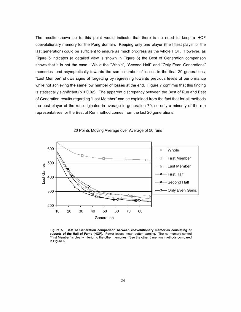
The results shown up to this point would indicate that there is no need to keep a HOF

coevolutionary memory for the Pong domain. Keeping only one player (the fittest player of the

last generation) could be sufficient to ensure as much progress as the whole HOF. However, as

Figure 5 indicates (a detailed view is shown in Figure 6) the Best of Generation comparison

shows that it is not the case. While the “Whole”, “Second Half” and “Only Even Generations”

memories tend asymptotically towards the same number of losses in the final 20 generations,

“Last Member” shows signs of forgetting by regressing towards previous levels of performance

while not achieving the same low number of losses at the end. Figure 7 confirms that this finding

is statistically significant (p < 0.02). The apparent discrepancy between the Best of Run and Best

of Generation results regarding “Last Member” can be explained from the fact that for all methods

the best player of the run originates in average in generation 70, so only a minority of the run

representatives for the Best of Run method comes from the last 20 generations.

20 Points Moving Average over Average of 50 runs

200

300

400

500

600

10 20 30 40 50 60 70 80

Generation

Lost Games

Whole

First Member

Last Member

First Half

Second Half

Only Even Gens.

Figure 5. Best of Generation comparison between coevolutionary memories consisting of subsets of the Hall of Fame (HOF). Fewer losses mean better learning. The no memory control “First Member” is clearly inferior to the other memories. See the other 5 memory methods compared in Figure 6.

25

20 Points Moving Average over Average of 50 runs (Zoomed In)

220

240

260

280

300

320

340

360

380

30 40 50 60 70 80

Generation

Lost Games Whole

Last Member

First Half

Second Half

Only Even Gens.

Figure 6. Detail of Figure 5. The “Last Member” memory shows a marked non-monotonic behavior that prevents it from achieving the final performance levels of the “Whole”, “Second Half” and “Only Even Generations” memories. This corresponds to forgetting, i.e. keeping only the latest evolved player is not enough to guarantee progress.

Average of 50 Runs over 20 Generation Intervals

0

100

200

300

400

500

600

700

0 - 19 20 - 39 40 - 59 60 - 79 80 - 99

Generation Interval

Lost Games

Whole

First Member

Last Member

First Half

Second Half

Only Even Gens.

Figure 7. Best of Generation comparison between coevolutionary memories consisting of subsets of the Hall of Fame (HOF). Fewer losses mean better learning. Losses are further averaged over 20 generation intervals. The vertical marks on top of the bars correspond to the

26

standard error. “Last Member” is significantly outperformed by “Whole”, “Second Half” and “Only Even Generations” in the last interval (p < 0.02), showing that forgetting is occurring in the last 20 generations, although not enough to be detected in the Best of Run comparison.

In conclusion, the two comparison methodologies complement each other and are accurate

enough to detect reasonable differences between coevolutionary memories with different sizes

and kinds of retention. Therefore, both comparisons will be used in the rest of the experiments.

The Pong domain can not provide general conclusions about the influence of the CM on player

performance because remembering the whole HOF does not evolve measurably better players

than remembering the last individual. Nevertheless, a statistically significant amount of forgetting

was detected in the last 20 generations, validating the need for the CMs.

4.2 Tracking Coevolution with the Growth of a Pareto Archive

Before using a Layered Pareto Archive as a Coevolutionary Memory, it is interesting to ask

whether its size can be used as a passive monitor to measure the success of a certain

coevolutionary memory at achieving better players. A CM that applies a higher selective

pressure should produce more Pareto dominant individuals in the same number of generations.

Since the archive retains a history of all the learners that were non-dominated in the past, its size

should be proportional to the selective pressure of the CM.

For each of the six HOF-based memories mentioned in Section 4.1, after every generation three

players were presented as tester candidates to a Layered Pareto Archive and three different

players were presented as learner candidates. The tester candidates were drawn randomly from

the population, whereas the learner candidates were the 3 fittest players belonging to three

different species in the population.

The average size of the learner and the tester sets of the archive at every generation are shown

in Figure 8. The first interesting result is that the learner set is consistently bigger than the tester

set (from around 50% in early generations to about 100% in the last ones). This fact has also

been reported by De Jong for the Compare-on-one problem (2004b). The figure corresponds to

the “Whole HOF” memory, but the results are similar for the other memories. Another

observation is that the Archive is an effective filter, since by generation 100 it has retained a

minority (an average of 37) of the 600 players presented.

27

Average over 50 runs

0

5

10

15

20

25

30

35

40

45

0 10 20 30 40 50 60 70 80 90

Generation

Size / Quantity

Archive

Learner Set

Tester Set

Layers of Learners

Species in Population

Figure 8. Growth of the Pareto Archive and its components when used as a monitor for the “Whole” HOF coevolutionary memory. The Pareto Archive is NOT used as a coevolutionary memory in this experiment but to monitor the progress of coevolution. The Learner Set is bigger and grows faster than the Tester Set. The number of Layers in the Learner Set is smaller and grows slightly slower than the Tester Set. Both facts are also true for the other 5 HOF variants considered. The archive ends up retaining an average of 37.6 players (with standard deviation of 6.3) out of 600 players presented as candidates. The fact that the rate of archive growth decreases over generations suggests that the update procedure detects the stagnation of the candidates presented.

Figure 9 shows that the archive grows in a relatively consistent way across the six different HOF-

based memories with two major exceptions. One is that for “First Member” the archive grows to

be substantially smaller than for the other memories. The other is that for “Second Half’ the

archive is significantly bigger than for “Last Member” during the last 3 intervals of 20 generations.

These two observations are coherent with Section 4.1 in which “First Member” and “Last

Member” had the worst performance and now their Pareto Archive monitors turns out to be

smaller. Hence the size of the Pareto Archive (averaged over 50 evolution runs) is related to the

corresponding coevolutionary progress.

28


0

5

10

15

20

25

30

35

40

45

0-19 20-39 40-59 60-79 80-99

Generation Interval

Archive Size

Whole

First Member

Last Member

First Half

Second Half

Only Even Gens.

Figure 9. Growth of the Pareto Archive when used as a monitor for the different HOF-based coevolutionary memories, further averaged over intervals of 20 generations. The vertical marks on top of the bars correspond to the standard error. The no-memory control “First Member” memory gets monitored by a substantially smaller archive, meaning that the archive update algorithm detects the smaller amount of innovation due to the low quality of the memory. The archive monitoring “Last Member” is significantly smaller than that of “Second Half” (p < 0.01) for the last 3 intervals, so the archive appears to detect the extra selective pressure due to the higher diversity of the “Second Half” memory that prevents forgetting.

In summary, in the Pong domain the LAPCA algorithm keeps few players and the quantity of

players kept is in agreement with the performance of the evolved players, when it is used as a

monitor for other CMs.

4.3 Introducing Candidates to the Pareto Archive

After having analyzed the performance of HOF-based coevolutionary memories and of the Pareto

Archive as a monitor, the next experiment introduces the Pareto Archive as a coevolutionary

memory. The whole archive (the union of the learner and tester sets) was used to extract

evaluators, i.e. to measure the fitness of the evolving individuals.

To use a Pareto Archive in the most effective way as a coevolutionary memory, it is necessary to

determine which individuals from the population, when presented as candidates, produce the best

archive as measured by a higher selective pressure and therefore superior players evolved. It

29

makes sense to present candidate individuals from different species to exploit the diversity in the

speciation mechanism of NEAT. However, selecting only the fittest players of different species

could produce a bias towards strategies that win on average, which may in turn prevent

idiosyncratic players from joining the archive. Such lost idiosyncratic players could have had

strategies that worked extremely well in specific situations and would have raised the selective

pressure of the archive. In other words, fitness alone might not be the best criterion to present

individuals to the archive, since it could be diversity that matters most.

The second experiment compares two kinds of candidate introduction: “Random” and “Top”.

“Random” corresponds to choosing three individuals from a uniform sample of the population,

disregarding species and fitness. “Top” corresponds to choosing the three fittest individuals in

the population that belong to different species. Since these two types of candidate introduction

can be applied independently to the tester and the learner sets, there are four combinations.

The six possible pairwise comparisons between the four types of candidate introduction appear

on Table 2, using the Best of Run method. There are only two statistically significant

comparisons: “Random Learners and Random Testers” are outperformed by “Top Learners and

Top Testers” and also by “Random Learners and Top Testers”. The consequence is that

candidate fitness is more important than candidate diversity at least for the Pong domain studied.

This result is supported by the fact that “Top Learners and Top Testers” introduces less diversity

to the archive than the other three types of introduction. In “Top Learners and Top Testers” the

same three players are presented as tester and learner candidates, whereas in the other cases a

total of six different players are presented to the archive.

According to Figure 10 the performance gap between “Top Learners and Top Testers” and

“Random Learners and Random Testers” is biggest around generation 70, using the Best of

Generation comparison. Figure 11 confirms that the comparison is statistically significant.

In conclusion, at least in the Pong domain, it is better to introduce the fittest individuals to the

archive. Using random individuals to exploit their erratic behavior does not lead to a more solid

learning. For this reason, in all the following experiments that involve a LAPCA the candidates

introduced are the fittest of their respective species.

30

Comparison Method Dominated Players (Average)

Dominated Players (Std Dev)

Difference p value

Top Learners and Top Testers 49.30 15.81 1

Random Learners and Random Testers 43.98 14.51 5.32 0.040

Random Learners and Top Testers 48.82 15.27 2


Top Learners and Random Testers 48.40 17.26 3



Top Learners and Random Testers 44.92 16.20 3.08 0.162


Random Learners and Top Testers 45.06 15.51 2.58 0.197

Top Learners and Random Testers 47.26 16.56 6

Random Learners and Top Testers 45.48 14.85 1.78 0.286

Table 2. Best of Run pairwise comparison between different methods of presenting candidates to the Pareto Archive, using the Pareto Archive as the Coevolutionary Memory. Both the learner and tester candidates can be either the 3 fittest individuals in the Population belonging to three different species (Top), of just 3 individuals chosen at random from the Population (Random). The first two comparisons are statistically significant (p < 0.05). It is better to introduce top testers than random testers.

20 Points Moving Average over Average of 50 runs (Zoomed In)

240

260

280

300

320

340

30 40 50 60 70 80

Generation

Lost Games

Top Learners TopTesters

Top LearnersRandom Testers

Random LearnersTop Testers

Random LearnersRandom Testers

Figure 10. Best of Generation comparison between different methods of selecting candidates from the population to introduce to the Pareto Archive, using the Pareto Archive as the Coevolutionary Memory. Fewer losses mean better learning. “Top Learners and Top Testers” seems to have a clear lead over the other methods. See Figure 11 for statistical significance.

31


0

100

200

300

400

500

600

700

0 - 19 20 - 39 40 - 59 60 - 79 80 - 99

Generation Interval

Lost Games Random Learners Random Testers

Random Learners Top Testers

Top Learners Random Testers

Top Learners Top Testers

Figure 11. Best of Generation comparison between different methods of selecting candidates to the Pareto Archive when used as the Coevolutionary Memory. Losses are further averaged over 20 generation intervals. Fewer losses mean better learning. The vertical marks on top of the bars correspond to the standard error. “Top Learners Top Testers” is significantly better (p < 0.02) than “Random Learners Random Testers” in the interval 60-79. “Top Learners Top Testers” is also better (p < 0.05) than “Top Learners Random Testers” in the same interval.

4.4 Extracting Evaluators from the Pareto Archive

The second question regarding the most efficient way to use the Pareto Archive as a

Coevolutionary Memory is: which individuals within the Archive are more useful to evaluate

fitness against?

Using the results of the previous section, the three fittest players belonging to different species

were presented as both learner and tester candidates to four implementations of the Pareto

Archive in which different subsets of the Archive were used to extract evaluators, that is, to obtain

a sample of players against which to measure the fitness of the evolving players. The four

extraction subsets were: “Archive” for the whole archive, “Learners” and “Testers” for the leaner

and tester sets and “Layer 1” for the outermost non-dominated layer of learners (the Pareto set).

32

Comparison Method Dominated Players (Average)

Dominated Players (Std Dev)

Difference p value

Archive 49.72 16.45 1

Learners 43.86 18.13 5.86 0.045

Layer 1 48.78 15.27 2

Learners 44.48 18.42 4.30 0.102

Testers 48.06 13.76 3

Learners 44.88 19.28 3.18 0.171

Layer 1 46.74 15.82 4

Archive 45.52 15.38 1.22 0.348

Archive 46.54 16.12 5

Testers 46.24 14.41 0.30 0.461

Testers 46.26 13.87 6

Layer 1 46.00 15.06 0.26 0.464

Table 3. Best of Run pairwise comparison between the different components of the Pareto Archive when they are used as the Coevolutionary Memory. Using the whole archive is better (p < 0.05) than using the learners only.

The results of the Best of Run comparison methodology are shown in Table 3. The only

statistically significant comparison is that it is better to use the whole archive than just the

learners. Since the same candidates were presented to both the learner and the tester set, and

since the archive is the union of learners and testers it follows that the testers are the most

important part of the archive. However, the testers do not outperform the learners in direct

comparison (third row). The learners, although not as valuable as the testers, offer an advantage

to the archive.

33

20 Pts Moving Average over Average of 50 runs (Zoomed In)

240

250

260

270

280

290

300

310

320

330

340

350

30 40 50 60 70 80

Generation

Lost Games

Archive

Learners

Testers

Layer 1

Figure 12. Best of Generation comparison between the different components of the Pareto Archive when used to provide fitness evaluators. Fewer losses mean better learning. “Layer 1” seems to have worse performance than the other methods in earlier generations. “Testers” seems to do better than the rest in later generations. However, these comparisons are not statistically significant (See Figure 13)

The results of the Best of Generation comparison from Figure 12 suggest that the testers may

become increasingly useful as evaluators in later generations. However, Figure 13 indicates that

the performance difference is so small that gets masked by the standard error of the

measurements. Another possible speculation is that “Layer 1” is not as good as any of the other

methods, reinforcing the fact that the testers contain more valuable information than even the

non-dominated layer of learners.

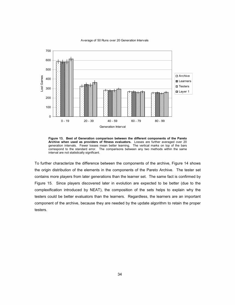
34


0

100

200

300

400

500

600

700

0 - 19 20 - 39 40 - 59 60 - 79 80 - 99

Generation Interval

Lost Games Archive

Learners

Testers

Layer 1

Figure 13. Best of Generation comparison between the different components of the Pareto Archive when used as providers of fitness evaluators. Losses are further averaged over 20 generation intervals. Fewer losses mean better learning. The vertical marks on top of the bars correspond to the standard error. The comparisons between any two methods within the same interval are not statistically significant.

To further characterize the difference between the components of the archive, Figure 14 shows

the origin distribution of the elements in the components of the Pareto Archive. The tester set

contains more players from later generations than the learner set. The same fact is confirmed by

Figure 15. Since players discovered later in evolution are expected to be better (due to the

complexification introduced by NEAT), the composition of the sets helps to explain why the

testers could be better evaluators than the learners. Regardless, the learners are an important

component of the archive, because they are needed by the update algorithm to retain the proper

testers.

35

Average over 50 runs

0

1

2

3

4

5

6

7

8

9

10

0 10 20 30 40 50 60 70 80 90 100

Generation Interval in which Player Originated

Number of Players Retained

Archive

Learners

Testers

Layer 1

Figure 14. Distribution of player origin for the different components of the Pareto Archive. The distribution depicted corresponds to the archive at generation 100, but snapshots at earlier generations show a similar profile. The learner set retains candidates mostly from earlier generations, whereas the tester set retains more candidates from initial and final generations. The outermost layer of learners “Layer 1” contains mostly players from later generations but not as recent as the tester set, as shown in Figure 15.

In conclusion, although the differences between different methods of candidate extraction are not

significant enough to establish that the testers alone are the best evaluators, there are indications

that the tester set has a higher diversity and more recent players than both the learner set and

the first non-dominated layer of learners, while having an intermediate size between the two.

Therefore, similar experiments in different domains are needed to determine whether the testers

are better evaluators by themselves, or if a combination with the Pareto front or with the whole

archive has a higher selective pressure. To take advantage of the only significant result, the

evaluators for the final experiment were drawn from a uniform sample of the whole archive.

36

Average over 50 Runs

0

10

20

30

40

50

60

70

80

90

100

Archive Learners Testers Layer 1

Pareto Archive Component

Generation of Origin

Max

Average

Min

Figure 15. Generation of origin (average and range) for the elements of the different components in the Pareto Archive. The vertical brackets are the standard error of the 50 run average (most of them are too small to be seen). Although “Layer 1” gets in average more players from higher generations than “Testers”, “Testers” contains more recently evolved players than “Layer 1”, i.e. has greater average of the maximum generation of origin. Hence the tester set seems to better represent the full strategy space.

4.5 Best of Generation Memory vs. Pareto Archive

The final experiment compares the performance of the Best of Generation (BOG) and Pareto

Archive coevolutionary memories, in three different aspects: performance of evolved players,

number of evaluations and storage size.

For each of the two memories, three different sizes of the candidate sets were evaluated: 1, 3

and “Sp”. Size “1” means that after every generation only the fittest player of the population is

either added to the BOG or presented to the Pareto Archive. Size “3” means that the candidates

are the three fittest players in the generation that belong to different species. Size “Sp” means

that one candidate from each species is presented to the memory, for all species in the

generation (there are 8 species in average in the last 40 generations). The HOF is the particular

case of a BOG memory with candidate size 1 (i.e., HOF is the same as “BOG – 1”) and is a good

baseline to judge the performance of the Pareto Archive.

37

Comparison Coevolutionary

Memory

Candidates per

Generation

Players Dominated (Average)

Players Dominated (Std Dev)

Diff p value

Pareto Archive Sp 48.46 13.98 1

BOG 3 43.86 14.22 4.60 0.051


BOG 1 (HOF) 44.86 15.30 2.86 0.163

Pareto Archive 3 47.72 14.90 3

BOG Sp 45.20 12.36 2.52 0.179


BOG Sp 44.90 13.91 2.32 0.205


Pareto Archive 1 45.50 14.84 1.40 0.312

BOG 3 46.74 16.42 6

BOG Sp 45.64 13.29 1.10 0.356


BOG 3 45.58 14.68 1.08 0.359


Pareto Archive 1 45.88 15.25 0.98 0.373

BOG 1 (HOF) 46.68 16.41 9

Pareto Archive 1 45.92 14.56 0.76 0.403

BOG Sp 46.44 13.08 10

BOG 1 (HOF) 45.72 16.24 0.72 0.404


Pareto Archive Sp 45.90 13.21 0.66 0.408

BOG Sp 46.80 13.40 12

Pareto Archive 1 46.16 16.72 0.64 0.416

BOG 1 (HOF) 46.52 14.87 13

Pareto Archive 3 46.28 15.49 0.24 0.468


BOG 3 46.50 15.10 0.22 0.471

BOG 3 46.22 14.29 15

BOG 1 (HOF) 46.10 15.34 0.12 0.484

Table 4. Best of Run pairwise comparison between the Best of Generation (BOG) and the Pareto Archive coevolutionary memories. The candidates can be the fittest individual from each generation (1), the top 3 fittest individuals belonging to different species (3), or the fittest individual of every species (Sp). As shown in Figure 8, during generations 60 to 100 the average number of species is 8.0 with standard deviation 1.5, so this is the number of candidates introduced in “Sp”. In the case of the Pareto Archive, using the results from section 4.4, the tester set is used to draw evaluators. The Pareto Archive with a candidate from every species is significantly better (p < 0.06) than the BOG memory with the top 3 fittest individuals from different species.

38

The performance of the two memories as measured by their evolved players is similar. However,

the larger candidate sets have an advantage over the smaller ones. Specifically, according to the

results of the Best of Run method from Table 4, “Pareto – Sp” has better performance than “BOG

– 3”. Also, from Figure 16 “BOG – 1 (HOF)” and “Pareto – 1” have the worst performance,

whereas from Figure 17 “BOG – Sp” is significantly better than “BOG – 1 (HOF)” around

generation 50.

20 Pts Moving Average over Average of 50 runs

240

260

280

300

320

340

30 40 50 60 70 80

Generation

Lost Games BOG -- 1 (HOF)

BOG -- 3

BOG -- Sp

Pareto -- 1

Pareto -- 3

Pareto -- Sp

Figure 16. Best of Generation comparison between the Best of Generation (BOG) and Pareto coevolutionary memories. Fewer losses mean better learning. The population candidates introduced to each memory (1, 3, Sp) are the same as in Table 4. “BOG -- 1 (HOF)” and “Pareto -- 1” produce the slowest learning, suggesting that presenting more than one candidate per generation increases selective pressure. However, as Figure 17 shows, only the comparison between “BOG -- Sp” and “BOG -- 1” (i.e., HOF) is statistically significant around generation 50.

39


0

100

200

300

400

500

600

700

0-19 20-39 40-59 60-79 80-99

Generation Interval

Lost Games

BOG -- 1 (HOF)

BOG -- 3

BOG -- Sp

Pareto -- 1

Pareto -- 3

Pareto -- Sp

Figure 17. Best of Generation comparison between the Best of Generation (BOG) and Pareto coevolutionary memories. Losses are further averaged over 20 generation intervals. Fewer losses mean better learning. The population candidates introduced to each memory (1, 3, Sp) are the same as in Table 4. The only statistically significant comparison is that “BOG -- Sp” is better than “BOG -- 1 (HOF)” (p < 0.05) in the generation interval 40-59. This improvement can be explained by faster initial growth of the “BOG – Sp” memory as it receives more candidates (see Figure 20).

In terms of number of evaluations, the Pareto archive has a clear disadvantage as shown in

Figure 18 per generation and in Figure 19 after 100 generations. The algorithm to implement any

BOG memory does not require evaluations, so evaluations are only needed to compute the

fitness of a newly created population. Since the population size is constant, the number of

evaluations per generation remains constant. Since the update algorithm of the Pareto Archive

needs to establish the dominance relationships between all candidates presented and all players

in the archive, the number of evaluations is not only proportional to the number of candidates but

also to the size of the archive, which increases monotonically.

40

Average of 50 runs

0

2000

4000

6000

8000

10000

12000

14000

16000

18000

0 10 20 30 40 50 60 70 80 90

Generation

Evaluations per Generation

Any BOG

Pareto -- 1

Pareto -- 3

Pareto -- Sp

Figure 18. Evaluations required per Generation by the BOG and Pareto Archive coevolutionary memories for different sizes of the sets of candidates. Coevolution with BOG memories needs a constant number of evaluations per generation: only to compute fitness. The update algorithm of the Pareto archive needs extra evaluations proportionally to the number of candidates and to the size of the archive. In the case of “Pareto – Sp” the vast majority of evaluations are used to update the archive. “Pareto – 1” and “Pareto – 3” balance better their evaluations between updating the archive and measuring fitness.

41


0

200,000

400,000

600,000

800,000

1,000,000

1,200,000

BOG

1 (HOF)

BOG

3

BOG

Sp

Pareto

1

Pareto

3

Pareto

Sp

Evaluations

Figure 19. Total evaluations required by the BOG and Pareto Archive coevolutionary memories after 100 generations for different sizes of the candidate sets. “Pareto-Sp” needs the most evaluations because it introduces more candidates and ends up with the biggest archive. Since all candidates have to play all the possible games against all the members of the archive, the number of evaluations grows dramatically. Keeping a BOG memory doesn’t require extra evaluations, since no players are filtered nor eliminated.

The advantage of the Pareto Archive is that it requires less storage. Figure 20 shows that the

archive retains a small proportion of the candidates introduced whereas the BOG memory by

definition keeps all the candidates presented. Figure 21 shows the memory sizes at generation

100. Because of the filtering of new candidates and the elimination of subsumed strategies

performed by the update procedure, the Pareto Archive requires less storage than the HOF and

the other BOG memories for all sizes of the candidate set. Since the performance of the six

methods is similar to each other (Figure 17) the Pareto Archive reduces the redundancy present

in the BOG memories without sacrificing performance.

42

Average of 50 runs

0

20

40

60

80

100

120

140

160

0 10 20 30 40 50 60 70 80 90

Generation

Quantity / Size

Introduced -- 1

Introduced -- 3

Introduced -- Sp

Archive -- 1

Archive -- 3

Archive -- Sp

Figure 20. Relationship between the number of candidates introduced and the number retained by the Pareto Archive, for different sizes of the sets of candidates. Since the number of candidates introduced to the archive coincides with the number of players added to the BOG memory, this also compares the growth of the BOG (“Introduced”) and Pareto Archive (“Archive”) coevolutionary memories. For the three candidate sizes (1, 3, Sp) the Pareto Archive grows slower than the HOF (i.e., “Introduced -- 1”). Also, although “Introduced -- Sp” gets more than six times bigger than “Introduced – 1” (see Figure 21), the corresponding archive “ Archive – Sp” gets less than 3 times bigger than “Archive – 1”.

43


0

100

200

300

400

500

600

700

800

BOG

1 (HOF)

BOG

3

BOG

Sp

Pareto

1

Pareto

3

Pareto

Sp

Final Memory Size

Figure 21. Size of the BOG and Pareto Archive coevolutionary memories at the end of 100 generations for different sizes of the candidate sets. Because of the filtering and elimination of the update procedure, the Pareto Archive requires less storage than the HOF and the other BOG memories for all candidate-set sizes. Since the performance of the six CMs is similar to each other (see Figure 17) the Pareto Archive reduces the redundancy present in the BOG memories without sacrificing performance.

In conclusion (Table 5), in the presented Pong domain the Pareto Archive is not significantly

better or worse than the Best of Generation coevolutionary memory in terms of performance of

the evolved players, but it uses less memory and requires more evaluations. In addition, in the

few cases in which there was a significant difference, multiple candidates per generation

produced better results than one, suggesting that the Hall of Fame can be outperformed when the

diversity present on the population is exploited.

44

Candidates Introduced

Final Memory Size

Evaluations Coevolutionary Memory

Average Std Dev Average Std Dev Average Std Dev

BOG -- 1 (HOF) 100 0.0 100 0.0 200,000 0

BOG – 3 300 0.0 300 0.0 200,000 0

BOG -- Sp 630 73.1 630 73.1 200,000 0

Pareto -- 1 100 0.0 20 3.77 262,478 10,691

Pareto -- 3 300 0.0 38 6.18 503,392 39,026

Pareto -- Sp 618 64.4 45 8.97 1,000,838 135,341

Table 5. Evaluations vs. Memory size trade-off between the BOG and Pareto Archive coevolutionary memories. A greater number of candidates per generation presented to any memory leads to better performance (according to Table 4 and Figure 17). Whereas in a BOG memory more candidates lead to a bloated CM without the cost of additional evaluations, a Pareto Archive with more candidates requires more evaluations but uses less storage.

45

5. DISCUSSION AND FUTURE WORK

The Best of Run and Best of Generation comparison methodologies were sensitive enough to

detect forgetting in the Pong domain (Section 4.1). In particular, the Best of Run comparison

established that a coevolutionary memory that by the n-th generation only remembers individuals

from the first n / 2 generations (a form of short-term forgetting) evolves players that are

significantly outperformed by those evolved with a HOF memory. In addition, the Best of

Generation comparison revealed that remembering only the last generation (long-term forgetting)

leads to regression: the quality of the players improves non-monotonically, especially in the last

20 generations. Each instance of forgetting was detected by one comparison methodology but

overlooked by the other, demonstrating that the two comparisons complement each other.

The amount of forgetting was insufficient to make strong claims about the selective pressure of

the LAPCA coevolutionary memory compared to the HOF. There was no measurable difference

in the average quality of the players evolved either with a CM with only one element (the fittest

individual of the generation immediately before) or with the full HOF. Therefore, it is impossible to

argue the practical advantage of a memory with two or more individuals. The experiments

described in this thesis should be repeated in a domain that experiences more coevolutionary

forgetting. A good criterion to make sure that such domain allows meaningful comparisons is

precisely the difference in the performance of players evolved remembering either the last or all

members of the HOF.

The lack of forgetting in the Pong domain can be attributed to many reasons: the board may be

too small; the physics may be too simple; using absolute coordinates as network inputs instead of

radar sensors may favor location-dependent strategies over general ones; giving players no more

than three options to deflect the ball may be too easy to predict by the opponent, etc. Changing

these parameters can lead to a bigger strategy space and to more coevolutionary forgetting. It

could also be that the intrinsic nature of the game allows a single player to dominate all possible

adversaries, in which case such a player is all that needs to be kept in the CM. For example, it

might be the case that an actual ping-pong player has a level of ability that makes him or her

undefeatable. If that is the case for Pong, it would be necessary to repeat these experiments in a

completely different domain.

46

In spite of the strategic simplicity of the Pong domain, the experiments draw some valid

conclusions about the implementation of the Layered Pareto Archive as a CM for the coevolution

of neural networks, and about the interaction between the LAPCA and NEAT. One conclusion is

that there is a positive, measurable impact from feeding the archive with candidates that are the

fittest within their species, as opposed to randomly sampling candidates from the population

(Section 4.3). Along the same lines, in the few comparisons that had statistical significance, the

bigger number of generational candidates corresponded to faster or better evolution (Section

4.5). Consequently, a CM can take advantage of the population diversity maintained by

speciation, and the best way to do it is by introducing the fittest individuals from different species.

Another observation is that the tester set has a more balanced and diverse composition than the

learner set, and that it is an important source of evaluators in the Pareto archive. Whereas the

learner set contains a majority of individuals originated in the first half of evolution, the tester set

has a more symmetric profile (Figure 14) and is likely to include players from more recent

generations (Figure 15). An important conclusion is that the number of evaluations required by

the update procedure of the LAPCA is practical for real world applications. The number of

evaluations per generation needed by the archive update algorithm is proportional to the number

of candidates and to the size of the archive. The archive does not grow too fast, because many

old players get subsumed by newer players and are immediately removed. The number of

candidates per generation is arbitrarily set by the experimenter. Hence, it is possible to adjust the

number of evaluations needed to update the archive to have it in the same order of magnitude as

the number of evaluations needed by NEAT to compute fitness (Section 4.5).

In his presentation of the LAPCA algorithm, De Jong (2004) used the archive in a different way

than how it was used in this thesis: not to provide evaluation for the population, but to re-

introduce genetic material into it. Such genotypical use of the archive could be implemented with

NEAT. Although it might interfere with the stability of NEAT’s speciation mechanism or potentially

stifle complexification, re-introducing previous genomes might give them a second chance to

evolve into the most successful players for the new competitive environment.

A central simplification in this thesis is that only one population coevolves, and does so by

competing against its own coevolutionary memory. It was argued that there was no need for a

second population because the population contained a sufficient number of species to evolve

diverse strategies simultaneously. Coevolving a single population against itself is a departure

from the way coevolution has been implemented in the past. In other symmetric domains like the

47

robot duel and compare-on-one, the two players are evolved in different populations, each with its

own coevolutionary memory (Stanley & Miikkulainen, 2004; De Jong, 2004). It would be

interesting to measure the impact of merging the two populations as it was done here.

In order to make fair comparisons between different CMs, the best of run individuals were always

the winners of an internal master tournament among generation champions. Nevertheless, since

the LAPCA memory contains dominance information about the players, the winner should be

drawn directly from archive, with no need for a master tournament. The natural choice would be

one of the learners in the Pareto front (first non-dominated layer). However, since the testers

contain more recently evolved individuals, one of them could be a better choice. Which individual

to choose and whether it has better performance than the winner of the master tournament is an

interesting question for future work.

There are alternative methods of coevolution that should be applied to neural networks. One

variation is replacing the solution concept of the Pareto Front by that of Nash equilibrium, using

the Nash memory mechanism proposed by Ficici and Pollack (2003). Another possibility is to

apply one or both solution concepts to neural network controllers for team competitive games like

soccer, in which the interaction between teammates introduces cooperation to coevolution.

The automated search for good players provided by coevolution has practical applications that

should also be investigated. In a videogame, the artificial intelligence of an agent could improve

more and faster by competing against other agents than by human instruction. Domains like the

interaction between viruses and immune systems or between computer security systems and

attackers can be modeled as a game in software. The automatic computation of optimal

opponents in such domains would make it possible to discover the best defensive strategies

without having to learn them in real life. The results obtained in this thesis are encouraging

because they show that the principles of Pareto coevolution can be applied to practical domains.

The computational expense of keeping an archive could be offset by a more effective or faster

evolution that reduces the overall number of evaluations and makes coevolution practical for real

world applications.

48

6. CONCLUSION

The main goal of this thesis was to construct a bridge between two branches of the study of

coevolution that have not been investigated together. The first branch comes from

neuroevolution and is very practical: coevolving optimal neural network controllers using the

fewest number of evaluations. The computational simplicity of maintaining a Hall of Fame (which

does not require evaluations) has made it the coevolutionary memory of choice for the

competitive coevolution of neural networks. The second branch comes from the theoretical

analysis of coevolution seen as multi-objective optimization: implementing an ideal coevolutionary

memory. Such a memory requires many evaluations to make explicit the Pareto-dominance

relationship between evolving individuals. The recently introduced LAPCA algorithm (De Jong,

2004b) decreases the number of evaluations needed to approximate a good coevolutionary

memory. However, it has only been applied to a Numbers Game which is not a very practical

domain.

This thesis implemented LAPCA as the coevolutionary memory for neural networks that control

the players of the game Pong. The evolutionary algorithm chosen was NEAT (Stanley &

Miikkulainen, 2002a) because its speciation and complexification features have already been

found useful for continual coevolution. The question on whether coevolution can discover better

solutions using a LAPCA memory than using a HOF memory remains open because there is not

enough forgetting in the Pong domain. However, three interesting results were encountered in

the effort. The first is a practical technique to provide generational candidates to a CM: choose

the fittest individuals that belong to different species. In the Pong domain this technique brings

more information to the memory than introducing the single best player of the generation, and is

more effective than introducing a random sample with the same size. The second result is that

the LAPCA behaves similarly in a complex neural network domain to how it does in the simpler

numeric domain. When applied to the evolution of neural networks, the bounded growth of the

archive makes the LAPCA a feasible option in terms of total number of evaluations. Third, in all

experiments performed, the LAPCA required significantly less memory than the HOF. Therefore,

LAPCA has a storage advantage in applications in which evolution lasts for many generations.

In sum, LAPCA has been demonstrated to be a practical CM for neural networks in the Pong

domain. Further research in domains that are more susceptible to forgetting is necessary to

determine whether it also allows discovering solutions that perform better. Eventually it should be

49

possible to establish the circumstances under which each of the two algorithms provides a better

CM for a given real-world application.

50

REFERENCES

Adams, E. A. (2005). The CheetahSpot: Locomotion. Retrieved August 6, 2005, from

http://www.cheetahspot.com/speed.php

Ahl, D. (1976). Playing Pong to win. The Best of Creative Computing, 1, 141. Retrieved August 6,

2005, from http://www.atariarchives.org/bcc1/showpage.php?page=141

Cliff, D., & Miller, G. (1995). Tracking the red queen: Measurements of adaptive progress in

coevolutionary simulations. Proceedings of the Third European Conference on Artificial

Life, 200-218.

Cohen, P. R. (1995). Empirical methods for artificial intelligence. MIT Press.

De Jong, E. D. (2004a). The incremental Pareto-coevolution archive. Proceedings of the Genetic

and Evolutionary Computation Conference, 525-536.

De Jong, E. D. (2004b). Towards a bounded Pareto-coevolution archive. Proceedings of the

Congress on Evolutionary Computation CEC-04.

De Jong, E. D., & Pollack, J. B. (2003). Learning the ideal evaluation function. Proceedings of the

2003 Genetic and Evolutionary Computation Conference, 277-288.

De Jong, E. D., & Pollack, J. B. (2004). Ideal evaluation from coevolution. Evolutionary

Computation, 12(2), 159-192.

Ficici, S. G. (2004). Solution concepts in coevolutionary algorithms. Dissertation Abstracts

International, 65 (03), 1399B.

Ficici, S. G., & Pollack, J. B. (2000). A game-theoretic approach to the simple coevolutionary

algorithm. Parallel Problem Solving From Nature (PPS-VI), 1917.

Ficici, S. G., & Pollack, J. B. (2003). A game-theoretic memory mechanism for coevolution.

Proceedings of the 2003 Genetic and Evolutionary Computation Conference, 286-297.

Floreano, D., & Nolfi, S. (1997). God save the Red Queen! Competition in co-evolutionary

robotics. Evolutionary Computation, 5.

Klooster, E. (n.d.). History of home and game computers: Atari’s Pong a legend begins. Retrieved

August 6, 2005, from http://computermuseum.50megs.com/pong.htm

MacIsaac, J. (2004, December 17). Remembering the first video game. Digital Journal. Retrieved

August 6, 2005, from http://www.digitaljournal.com/news/?articleID=4162

Moriarty, D. E., Schultz, A. C., & Grefenstette, J. J. (1999). Evolutionary algorithms for

reinforcement learning. Journal of Artificial Intelligence Research, 11, 241-276.

51

Noble, J., & Watson, R. A. (2001). Pareto coevolution: Using performance against coevolved

opponents in a game as dimensions for Pareto selection. Proceedings of the Genetic and

Evolutionary Computation Conference, GECCO-2001, 493-500.

Poppleton, T. (2002). Can co-evolution play ball? Competitive co-evolution in a Pong game.

Unpublished master’s thesis, University of Sussex, UK. Retrieved August 6, 2005, from

http://www.informatics.susx.ac.uk/easy/Publications/Online/MSc2002/ajp25.pdf

Rosin, C. D., & Belew, R. K. (1997). New methods for competitive evolution. Evolutionary

Computation, 5.

Russell, S., & Norvig, P. (2003). Artificial intelligence: A modern approach (2nd ed., pp.

32,161-163, 763-764). Prentice Hall.

Stanley, K., Bryant, B. D., & Miikkulainen, R. (2005). Evolving neural network agents in the NERO

videogame. Proceedings of the IEEE 2005 Symposium on Computational Intelligence

and Games (CIG’05).

Stanley, K. O., & Miikkulainen, R. (2002a). Evolving neural networks through augmenting

topologies. Evolution, 10(2), 99-127.

Stanley, K. O., & Miikkulainen, R. (2002b). Efficient evolution of neural network topologies.

Proceedings of the 2002 Congress on Evolutionary Computation (CEC ‘02).

Stanley, K. O., & Miikkulainen, R. (2002c). Efficient reinforcement learning through evolving

neural network topologies. Proceedings of the Genetic and Evolutionary Computation

Conference (GECCO-2002).

Stanley, K. O., & Miikkulainen, R. (2002d). Continual coevolution through complexification.

Proceedings of the Genetic and Evolutionary Computation Conference (GECCO-2002).

Stanley, K. O., & Miikkulainen, R. (2003). Achieving high-level functionality through

Complexification. Proceedings of the AAAI-2003 Spring Symposium on Computational

Synthesis.

Stanley, K. O., & Miikkulainen, R. (2004). Competitive coevolution through evolutionary

complexification. Journal of Artificial Intelligence Research, 21, 63-100.

Winter, D. (2005). Magnavox Odyssey: First home video game console. Retrieved August 6,

2005, from http://www.pong-story.com/odyssey.htm

52

VITA

German Alberto Monroy was born in Duitama (Boyacá), Colombia on February

11, 1975, the first child of German Monroy Rojas and Flor Alba Alvarez de

Monroy. He has a sister called Silvia and a brother called Diego Alejandro. After

attending high school at the Colegio Seminario Diocesano in Duitama, in 1992 he

entered the Pontificia Universidad Javeriana in Bogotá, Colombia. In 1996 he

did a 6-month internship in IT at NCR Colombia. He received the degree of

Bachelor of Science in Electronic Engineering from Universidad Javeriana in

1997. After two short jobs working as contractor, he joined Intel Tecnología de

Colombia in Bogotá as an Applications Engineer, for three and a half years until

2002. During four semesters in 1997, 2002 and 2003 he was also an instructor

at his alma mater. In August, 2003, he entered The Graduate School at The

University of Texas.

Permanent Address: 5830 SW Hall Blvd

Beaverton, OR 97005

This thesis was typed by the author.

Copyright by German A. Monroy 2005nn.cs.utexas.edu/downloads/papers/monroy.thesis05.pdf · by...

Documents

Transcript of Copyright by German A. Monroy 2005nn.cs.utexas.edu/downloads/papers/monroy.thesis05.pdf · by...