Copyright © 2009 Cengage Learning 19.1 Chapter 19 Nonparametric Statistics.
96
Copyright © 2009 Cengage Learning 19.1 Chapter 19 Nonparametric Statistics
-
Upload
robyn-dickerson -
Category
Documents
-
view
213 -
download
0
Transcript of Copyright © 2009 Cengage Learning 19.1 Chapter 19 Nonparametric Statistics.

Copyright © 2009 Cengage Learning 19.1
Chapter 19
Nonparametric Statistics

Copyright © 2009 Cengage Learning 19.2
Nonparametric StatisticsThis chapter deals with statistical techniques that deal with ordinal data.
Ordinal data is the result of a rating system such as
Excellent, good, fair, and poor
W can record the responses using any numbering system as long as the order is maintained. For example,
Excellent = 4Good = 3Fair = 2Poor = 1

Copyright © 2009 Cengage Learning 19.3
Ordinal Data…or
Excellent = 85Good = 40Fair = 25Poor = 10
Both numbering systems are valid.

Copyright © 2009 Cengage Learning 19.4
Ordinal Data…The difference between interval and ordinal data is that with interval data the differences are meaningful and consistent. With ordinal data the differences between values has no meaning. For example, what is the difference between Excellent and Good. Is it
4-3 = 1 ? or
85-40 = 45 ?
The answer is neither. All we can say about the difference between Excellent and Good is that Excellent is ranked higher. We cannot interpret the magnitude of the difference.

Copyright © 2009 Cengage Learning 19.5
Nonparametric StatisticsWhen the data are ordinal, the mean is not an appropriate measure of central location.
Instead, we will test characteristics of populations without referring to specific parameters, hence the term nonparametric.
Although nonparametric methods are designed to test ordinal data, they have another area of application.
The statistical tests described in Sections 13.1 and 13.3 and in Chapter 14 require that the populations be normally distributed.

Copyright © 2009 Cengage Learning 19.6
Nonparametric Statistics
If the data are extremely nonnormal, the t-tests and F-test are invalid.
Nonparametric techniques can be used instead.
For this reason, nonparametric procedures are often (perhaps more accurately) called distribution-free statistics.
Copyright © 2009 Cengage Learning 19.7
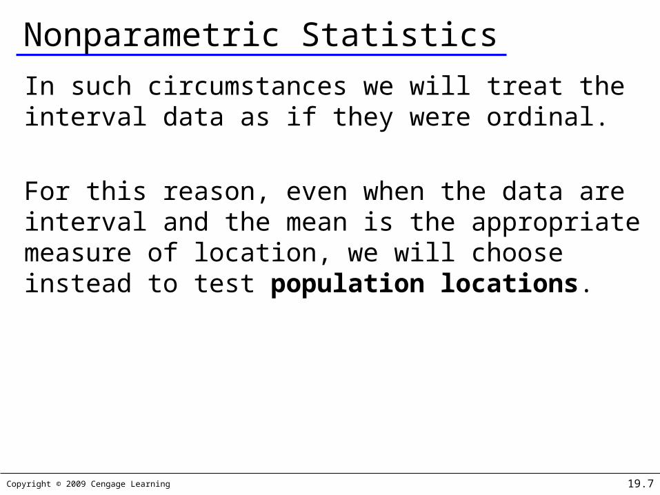
Nonparametric Statistics
In such circumstances we will treat the interval data as if they were ordinal.
For this reason, even when the data are interval and the mean is the appropriate measure of location, we will choose instead to test population locations.

Copyright © 2009 Cengage Learning 19.8
Population Locations
These two populations have the same location…
population 1
population 2

Copyright © 2009 Cengage Learning 19.9
Population LocationsThe location of pop’n 1 is to the left of the location of pop’n 2…
The location of pop’n 1 is to the right of the location of pop’n 2…
population 1 population 2
population 2 population 1

Copyright © 2009 Cengage Learning 19.10
Problem ObjectivesWhen the problem objective is to compare two populations the null hypothesis will state:
H0: The two population locations are the same.
The alternative hypothesis can take on any one of the following three forms:
H1: The location of population 1 is different from the location of population 2
H1: The location of population 1 is to the right of the location of population 2
H1: The location of population 1 is to the left of the location of population 2

Copyright © 2009 Cengage Learning 19.11
The Alternative Hypotheses
H1: The location of population 1 is different from the location of population 2
Used when we want to know whether there is sufficient evidence to infer that there is a difference between the two populations.

Copyright © 2009 Cengage Learning 19.12
The Alternative Hypotheses
H1: The location of population 1 is to the right of the location of population 2
Used when we want to know whether we can conclude that the random variable in population 1 is larger in general than the random variable in population 2,
and, not surprisingly…

Copyright © 2009 Cengage Learning 19.13
The Alternative Hypotheses H1: The location of population 1 is to the left of the location of population 2
Used when we want to know whether we can conclude that the random variable in population 1 is smaller in general than the random variable in population 2.
NOTE: all of our hypotheses are phrased in terms of “1 then 2”. This is for consistency. Rather than state:
H1: The location of population 2 is to the left of the location of population 2, we would want to phrase this as:
H1: The location of population 1 is to the right of the location of population 2

Copyright © 2009 Cengage Learning 19.14
Wilcoxon Rank Sum Test
We’ll use the Wilcoxon Rank Sum Test for problems where:
— Problem objective is to compare two populations,
— The data are ordinal or interval (where the normality requirement is unsatisfied)
— The samples are independent.

Copyright © 2009 Cengage Learning 19.15
Example 19.1From these samples:
: 22, 23, 20: 18, 27, 26 Can we conclude (at 5%
significance level) that the location of population 1 is to the left (i.e. “smaller”) that the location of population 2?
That is, we want to test:H0: The two population locations are the
same.H1: The location of population 1 is to the
left of the location of population 2.We can test this, we just need a test
statistic…

Copyright © 2009 Cengage Learning 19.16
Test Statistic
Step #1… rank the observations from smallest to largest, assign a rank number, and add up the “rank sum”…
rank rank
22 3 18 1
23 4 27 6
20 2 26 5
T1=9 T2=12
*in the case of “ties” we average the ranks
of the tied observations.
We arbitrarily select T1 as the test statistic and label it “T”

Copyright © 2009 Cengage Learning 19.17
Sampling Distribution of the Test StatisticA small value of T indicates most of the smaller observations are in sample 1 which was drawn from population 1 — but how small is “small”? Is 9 “small” enough?
We have our test statistic, T=9. We need to compare it to some critical value of “T” to know if we’re in the rejection region for H0 (or not).
So, what then, does the sampling distribution of “ranks” look like?

Copyright © 2009 Cengage Learning 19.18
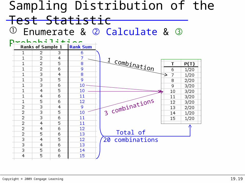
Sampling Distribution of the Test StatisticWe can build up the sampling distribution of the test statistic in much the same way we we built histograms for the outcomes of rolls of 2 and 3 dice…
Enumerate all possible combinations of ranks
Calculate ranks sums for the combinations
The probability of any rank sum is the number of occurrences divided by the total number of combinations…
Copyright © 2009 Cengage Learning 19.19
Sampling Distribution of the Test Statistic Enumerate & Calculate & Probabilities…
Total of20 combinations
1 combination
3 combinations

Copyright © 2009 Cengage Learning 19.20
X
Sampling Distribution of the Test Statistic
5%
P(T≤6) = 1/20 = .05Thus our critical value of T is 6
Since T=9 < TCritical=6, we cannotreject H0…

Copyright © 2009 Cengage Learning 19.21
Example 19.1…
We cannot reject the null hypothesis, that is, there is not enough evidence to conclude that the location of population 1 is located to the left of population 2 (at 5% significance).
INTERPRET

Copyright © 2009 Cengage Learning 19.22
Critical Values: Wilcoxon Rank Sum TestSample sizes less than 10 are unrealistic.
For sample sizes larger than 10, the test statistic is approximately normally distributed with:
Mean: Hence:
Standard Deviation:ni=size of sample i, i=1,2

Copyright © 2009 Cengage Learning 19.23
Example 19.2A pharmaceutical company is planning to introduce a new painkiller. In a preliminary experiment to determine its effectiveness, 30 people were randomly selected, of whom 15 were given the new painkiller and 15 were given aspirin. All 30 were told to use the drug when headaches or other minor pains occurred and to indicate which of the following statements most accurately represented the effectiveness of the drug they took. 5 = The drug was extremely effective. 4 = The drug was quite effective. 3 = The drug was somewhat effective. 2 = The drug was slightly effective. 1 = The drug was not at all effective.

Copyright © 2009 Cengage Learning 19.24
Example 19.2
The responses are listed here (and stored in Xm19-02) using the codes. Can we conclude at the 5% significance level that the new painkiller is perceived to be more effective? New painkiller: 3, 5, 4, 3, 2, 5, 1, 4, 5, 3, 3, 5, 5, 5, 4 Aspirin: 4, 1, 3, 2, 4, 1, 3, 4, 2, 2, 2, 4, 3, 4, 5

Copyright © 2009 Cengage Learning 19.25
Example 19.2The problem objective is to compare two populations. The data are ordinal and the samples are independent. The appropriate technique is the Wilcoxon rank sum test.
Its important to note here that “5” is a “good” score, so if the drug is effective, we’d likely see its location “greater than” the location of aspirin users, hence:
H1: The location of population 1 is to the right of the location of population 2, and so:
H0: The two population locations are the same.
IDENTIFY

Copyright © 2009 Cengage Learning 19.26
Example 19.2
(though not shown here) The rank sum for the new painkiller is T1=276.5, and the rank sum for aspirin: T2=188.5
Set T= T1=276.5, and begin calculating…
COMPUTE

Copyright © 2009 Cengage Learning 19.27
Example 19.2
The p-value of the test is:p-value = P(Z > 1.83) = .5 - .4664 =
.0336
(or Z=1.83 > Zα = Z.05 =1.645), hence:
“There is sufficient evidence to infer that the new painkiller is perceived to
be more effective than aspirin”
COMPUTE

Copyright © 2009 Cengage Learning 19.28
Example 19.2
We can use the Wilcoxon Rank Sum Test in the Data Analysis Plus set of tools to come to the same conclusion. Click Add-Ins, Data Analysis Plus, Wilcoxon Rank Sum Test.
COMPUTE

Copyright © 2009 Cengage Learning 19.29
Example 19.2
COMPUTE
p-value
12345678910
A B C DWilcoxon Rank Sum Test
Rank Sum ObservationsNew 276.5 15Aspirin 188.5 15z Stat 1.83P(Z<=z) one-tail 0.0340z Critical one-tail 1.6449P(Z<=z) two-tail 0.0680z Critical two-tail 1.9600

Copyright © 2009 Cengage Learning 19.30
Example 19.2There is enough evidence to infer that the new painkiller is more effective than aspirin.
INTERPRET

Copyright © 2009 Cengage Learning 19.31
Required ConditionsThe Wilcoxon rank sum test actually tests to determine whether the population distributions are identical. This means that it tests not only for identical locations, but for identical spreads (variances) and shapes (distributions) as well.
The rejection of the null hypothesis may be due instead to a difference in distribution shapes and/or spreads.
To avoid this problem, we will require that the two probability distributions be identical except with respect to location.

Copyright © 2009 Cengage Learning 19.32
Identifying Factors
Factors that identify the Wilcoxon Rank Sum…

Copyright © 2009 Cengage Learning 19.33
Tests for Matched Pairs ExperimentsWe will now look at two nonparametric techniques (Sign Test and Wilcoxon Signed Rank Sum Test) that test hypotheses in problems with the following characteristics:
— We want to compare two populations,— The data are either ordinal or
interval (nonnormal),— and the samples are matched pairs.
As before, we’ll compute matched pair differences and work from there…

Copyright © 2009 Cengage Learning 19.34
The Sign TestWe can use the Sign Test when we’re dealing with two populations of ordinal data in a matched pairs experiment.
For each matched pair, take the differences and count up the number of positive differences and negative differences.
If population locations are the same (say), we’d expect the number of positives and negatives to net out to zero. If we have more positives than negatives (or vice versa) what can we learn? Again, how many is enough to make a difference?

Copyright © 2009 Cengage Learning 19.35
Sign TestWe can think of the sign test in terms of a binomial experiment, getting a positive sign is like flipping heads on a coin. We use this notion along with previously developed statistics to come up with our standardized test statistic (assuming the null hypothesis is true):
Our null hypothesis:H0: the two population locations are the same
is equivalent to:H0: p = .5 (i.e. equal proportions of +’s &
–’s)
n≥10
Copyright © 2009 Cengage Learning 19.36
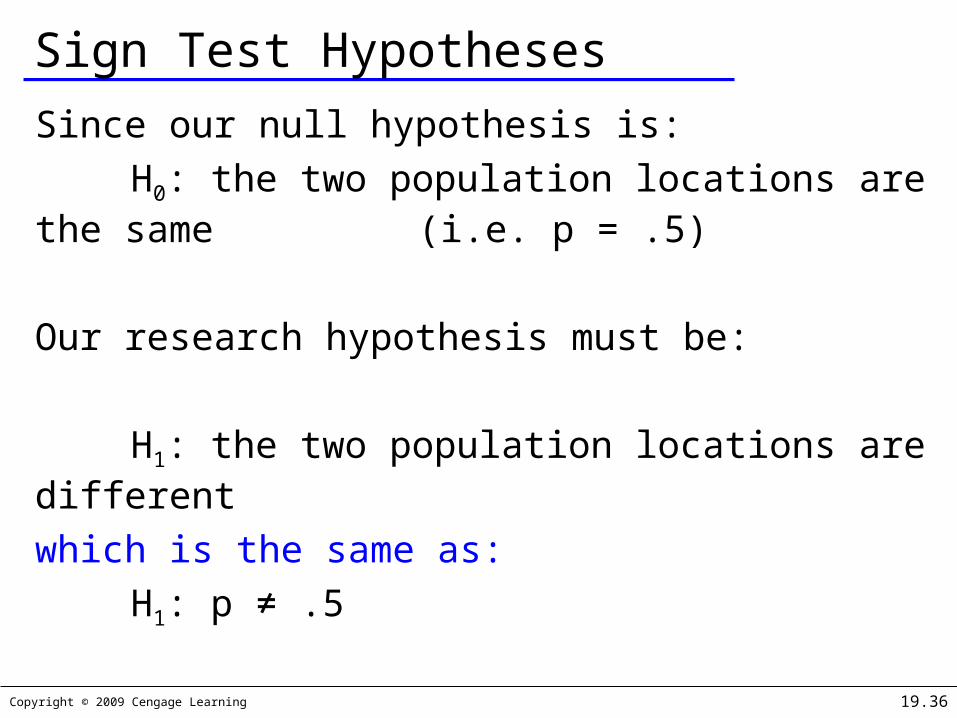
Sign Test Hypotheses
Since our null hypothesis is:H0: the two population locations are
the same (i.e. p = .5)
Our research hypothesis must be:
H1: the two population locations are differentwhich is the same as:
H1: p ≠ .5

Copyright © 2009 Cengage Learning 19.37
Example 19.3In an experiment to determine which of two cars is perceived to have the more comfortable ride, 25 people rode (separately) in the back seat of an expensive European model and also in the back seat of a North American midsize car. Each of the 25 people was asked to rate the ride on the following 5-point scale. 1 = Ride is very uncomfortable.2 = Ride is quite uncomfortable. 3 = Ride is neither uncomfortable nor comfortable. 4 = Ride is quite comfortable. 5 = Ride is very comfortable.The results are stored in Xm19-03. Do these data allow us to conclude at the 5% significance level that the European car is perceived to be more comfortable than the North American car?

Copyright © 2009 Cengage Learning 19.38
Example 19.3The problem objective is to compare two populations. The data are ordinal and the experimental design is matched pairs. Thus the correct technique is the sign test. Because we want to whether there is enough evidence to infer that the European car is perceived to have a smoother ride than the North American car the hypotheses are
H0 :The two population locations are the same.
H1 : The location of population 1 (European car rating) is to the right of the location of population 2 (North American car rating)
IDENTIFY

Copyright © 2009 Cengage Learning 19.39
Example 19.3
Again, we can leverage Excel to reduce the amount of work that we have to do. Click Add-Ins, Data Analysis Plus, Sign Test.
COMPUTE

Copyright © 2009 Cengage Learning 19.40
Example 19.3
COMPUTE
p-value
123456789101112
A B C D ESign Test
Difference European - American
Positive Differences 17Negative Differences 6Zero Differences 2z Stat 2.29P(Z<=z) one-tail 0.0109z Critical one-tail 1.6449P(Z<=z) two-tail 0.0218z Critical two-tail 1.9600

Copyright © 2009 Cengage Learning 19.41
Example 19.3There is enough evidence to infer that the European car is perceived to have a smoother ride than the North American car the hypotheses are
INTERPRET

Copyright © 2009 Cengage Learning 19.42
Checking the Required Conditions
The sign test requires: The populations be similar in
shape and spread:
The sample size exceeds 10 (n=23).
0
5
10
1 2 3 4 5Freq
uenc
y
North American Car Rating
Histogram
0
5
10
1 2 3 4 5Freq
uenc
y
European Car Rating
Histogram

Copyright © 2009 Cengage Learning 19.43
Wilcoxon Signed Rank Sum TestWe’ll use Wilcoxon Signed Rank Sum test when we want to compare two populations of interval (but not normally distributed) date in a matched pairs type experiment.
Compute paired differences, discard zeros. Rank absolute values of differences smallest (1) to largest (n), averaging ranks of tied observations. Sum the ranks of positive differences (T+) and of negative differences (T–). Use T=T+ as our test statistic…
Copyright © 2009 Cengage Learning 19.44
Wilcoxon Signed Rank Sum Test
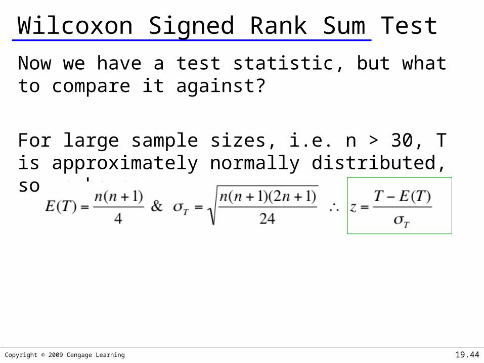
Now we have a test statistic, but what to compare it against?
For large sample sizes, i.e. n > 30, T is approximately normally distributed, so we have:

Copyright © 2009 Cengage Learning 19.45
Example 19.4Traffic congestion on roads and highways costs industry billions of dollars annually as workers struggle to get to and from work.
Several suggestions have been made about how to improve this situation, one of which is called flextime, which involves allowing workers to determine their own schedules (provided they work a full shift).
Such workers will likely choose an arrival and departure time to avoid rush-hour traffic.
Copyright © 2009 Cengage Learning 19.46
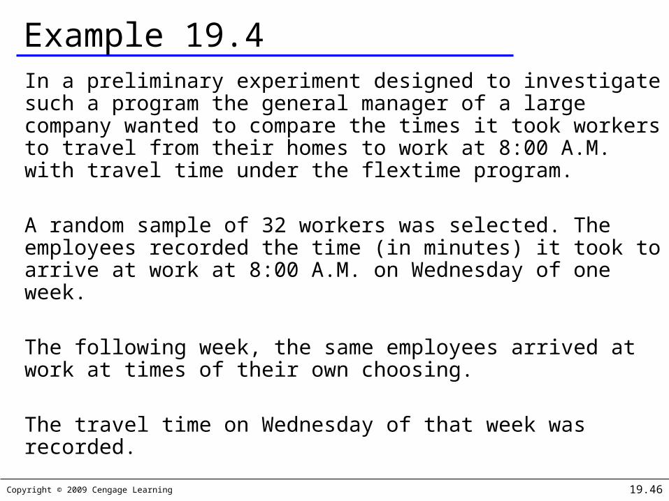
Example 19.4In a preliminary experiment designed to investigate such a program the general manager of a large company wanted to compare the times it took workers to travel from their homes to work at 8:00 A.M. with travel time under the flextime program.
A random sample of 32 workers was selected. The employees recorded the time (in minutes) it took to arrive at work at 8:00 A.M. on Wednesday of one week.
The following week, the same employees arrived at work at times of their own choosing.
The travel time on Wednesday of that week was recorded.

Copyright © 2009 Cengage Learning 19.47
Example 19.4
These results are listed in the Xm19-04. Can we conclude at the 5% significance level that travel times under the flextime program are different from travel times to arrive at work at 8:00 A.M.?

Copyright © 2009 Cengage Learning 19.48
Example 19.4The problem objective is to compare two populations. The data are interval and the samples are matched. If the matched pairs differences are normally distributed the correct method is the t-test of µD. Here is the histogram of the differences.
.
IDENTIFY

Copyright © 2009 Cengage Learning 19.49
Example 19.4
A histogram of the paired differences reveals a non-normal distribution, hence we must use a non-parametric technique.
IDENTIFY
0
5
10
-2 0 2 4 6Freq
uenc
y
Differences
Histogram

Copyright © 2009 Cengage Learning 19.50
Example 19.4The appropriate technique is the Wilcoxon signed rank sum test. Because we want to know whether the population locations differ we have
H0: The two population locations are the same.
H1: The two population locations are different
This is a two-tail test.
IDENTIFY
Copyright © 2009 Cengage Learning 19.51
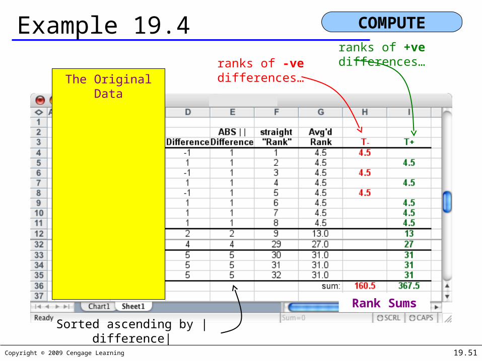
Example 19.4 COMPUTE
The Original Data
ranks of +ve differences…ranks of -ve
differences…
Rank Sums
Sorted ascending by |difference|

Copyright © 2009 Cengage Learning 19.52
Example 19.4
We compute our test statistic as follows…
Our rejection region is…
COMPUTE

Copyright © 2009 Cengage Learning 19.53
Example 19.4
Click Add-Ins, Data Analysis Plus, Wilcoxon Signed Rank Sum Test.
INTERPRETCOMPUTE

Copyright © 2009 Cengage Learning 19.54
Example 19.4
p-value
COMPUTE
123456789101112
A B CWilcoxon Signed Rank Sum Test
Difference 8:00-Arr - Flextime
T+ 367.5T- 160.5Observations (for test) 32z Stat 1.94P(Z<=z) one-tail 0.0265z Critical one-tail 1.6449P(Z<=z) two-tail 0.0530z Critical two-tail 1.9600

Copyright © 2009 Cengage Learning 19.55
Example 19.4
The Wilcoxon Signed Rank Sum Test tool in Data Analysis Plus yields the same result as the manual calculation; there is not enough evidence to infer that flextime commute times differ from 8:00 am start commute times.
INTERPRET

Copyright © 2009 Cengage Learning 19.56
Identifying Factors I
Factors that Identify the Sign Test…

Copyright © 2009 Cengage Learning 19.57
Identifying Factors II
Factors that Identify the Wilcoxon Signed Rank Sum Test…

Copyright © 2009 Cengage Learning 19.58
Kruskal-Wallis TestSo far we’ve been comparing locations of two populations, now we’ll look at comparing two or more populations.
The Kruskal-Wallis test is applied to problems where we want to compare two or more populations or ordinal or interval (but nonnormal) data from independent samples.
Our hypotheses will be:H0: The locations of all k populations are
the same.H1: At least two population locations
differ.

Copyright © 2009 Cengage Learning 19.59
Test Statistic
In order to calculate the Kruskal-Wallis test statistic, we need to:
Rank all the observations from smallest (1) to largest (n), and average the ranks in the case of ties. We calculate rank sums for each sample: T1, T2, …, Tk
Lastly, we calculate the test statistic (denoted H):

Copyright © 2009 Cengage Learning 19.60
Sampling Distribution of the Test Statistic:For sample sizes greater than or equal to 5, the test statistic H is approximately Chi-squared distributed with k–1 degrees of freedom.
Our rejection region is:
And our p-value is:

Copyright © 2009 Cengage Learning 19.61
Example 19.5The management of fast-food restaurants is extremely interested in knowing how their customers rate the quality of food and service and the cleanliness of the restaurants.
Customers are given the opportunity to fill out customer comment cards.
Suppose that one franchise wanted to compare how customers rate the three shifts
4:00 P.M. to midnightMidnight to 8:00 A.M.8:00 A.M. to 4:00 P.M

Copyright © 2009 Cengage Learning 19.62
Example 19.5In a preliminary study, 10 customer cards were randomly selected from each shift. The responses to the question concerning speed of service were recorded where
4 = excellent, 3 = good, 2 = fair, and 1 = poor
The data are listed next.
Do these data provide sufficient evidence at the 5% significance level to indicate whether customers perceive the speed of service to be different between the three shifts?
Copyright © 2009 Cengage Learning 19.63
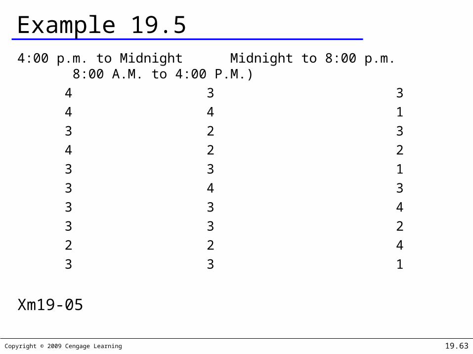
Example 19.54:00 p.m. to Midnight Midnight to 8:00 p.m. 8:00 A.M. to 4:00 P.M.)
4 3 34 4 13 2 34 2 23 3 13 4 33 3 43 3 22 2 43 3 1
Xm19-05

Copyright © 2009 Cengage Learning 19.64
Example 19.5The problem objective is to compare three populations of ordinal data (the ratings of the three shifts), and the samples are independent. These factors are sufficient to determine the use of the Kruskal-Wallis test. The null and alternative hypotheses are
H0:The locations of all three populations are the same.
H1: At least two population locations differ
IDENTIFY
Copyright © 2009 Cengage Learning 19.65
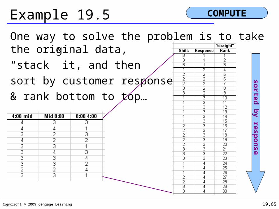
Example 19.5
One way to solve the problem is to take the original data,“stack” it, and thensort by customer response& rank bottom to top…
COMPUTEsorte
d b
y re
sp
on
se

Copyright © 2009 Cengage Learning 19.66
Example 19.5
Once its in “stacked” format, put in straight rankings from 1 to 30, average the rankings for the same response, then parse them out by shift to come up with rank sum totals…
COMPUTE

Copyright © 2009 Cengage Learning 19.67
Example 19.5
Our critical value of Chi-squared (5% significance and k–1=2 degrees of freedom) is 5.99, hence there is not enough evidence to reject H0.
COMPUTE

Copyright © 2009 Cengage Learning 19.68
Example 19.5From Data Analysis Plus, Kruskal Wallis a similar finding…
“There is not enough evidence to infer that a difference in speed of service exists between the three shifts, i.e. all three of the shifts are equally rated, and any action to improve
service should be applied to all three shifts”
COMPUTE
p-value

Copyright © 2009 Cengage Learning 19.69
Identifying Factors
Factors that Identify the Kruskal-Wallis Test…

Copyright © 2009 Cengage Learning 19.70
Friedman TestThe Friedman Test is a technique used compare two or more populations of ordinal or interval (nonnormal) data that are generated from a randomized block experiment.
The hypotheses are the same as in the Kruskal-Wallis test.
H0: The locations of all k populations are the same.
H1: At least two population locations differ.

Copyright © 2009 Cengage Learning 19.71
Friedman Test – Test StatisticSince this is a blocked experiment, we first rank each observation within each of b blocks from smallest to largest (i.e. from 1 to k), averaging any ties. We then compute the rank sums: T1, T2, …, Tk. The we calculate our test statistic:
This test statistic is approximate Chi-squared with k–1 degrees of freedom (provided either k or b ≥ 5). Our rejection region and p-value are:

Copyright © 2009 Cengage Learning 19.72
Example 19.6The personnel manager of a national accounting firm has been receiving complaints from senior managers about the quality of recent hirings. All new accountants are hired through a process whereby four managers interview the candidate and rate her or him on several dimensions, including academic credentials, previous work experience, and personal suitability. Each manager then summarizes the results and produces an evaluation of the candidate. There are five possibilities:1 The candidate is in the top 5% of applicants.2 The candidate is in the top 10% of applicants, but not in the top 5%.3 The candidate is in the top 25% of applicants, but not in the top 10%.4 The candidate is in the top 50% of applicants, but not in the top 25%.5 The candidate is in the bottom 50% of applicants.

Copyright © 2009 Cengage Learning 19.73
Example 19.6The evaluations are then combined in making the final decision. The personnel manager believes that the quality problem is caused by the evaluation system. However, she needs to know whether there is general agreement or disagreement between the interviewing managers in their evaluations. To test for differences between the managers, she takes a random sample of the evaluations of eight applicants. The results are shown below and stored in Xm19-06. What conclusions can the personnel manager draw from these data? Employ a 5% significance level.

Copyright © 2009 Cengage Learning 19.74
Example 19.6
ManagerApplicant 1 2 3 41 2 1 2 22 4 2 3 23 2 2 2 34 3 1 3 25 3 2 3 56 2 2 3 47 4 1 5 58 3 2 5 3

Copyright © 2009 Cengage Learning 19.75
Example 19.6The problem objective is to compare the four populations of managers' evaluations, which we can see are ordinal data. This experiment is identified as a randomized block design because the eight applicants were evaluated by all four managers. (The treatments are the managers, and the blocks are the applicants.) The appropriate statistical technique is the Friedman test. The null and alternative hypotheses are as follows.
H0: The locations of all four populations are the same
H1: At least two population locations differ
IDENTIFY

Copyright © 2009 Cengage Learning 19.76
Example 19.6The data looks like this:
Applicant #1 for example, received a top score from manager and next-to-top scores from the other three.Applicant #7 received a top score from manager as well, but the other three scored this candidate very low…
COMPUTE
There are k=4 populations (managers) and b=8 blocks (applicants) in this set-up.

Copyright © 2009 Cengage Learning 19.77
Example 19.6
“rank each observation within block from smallest to largest (i.e. from 1 to k), averaging any ties”… For example, consider the case of candidate #2:
COMPUTE
Manager
Manager
Manager
Manager
Original Scores 4 2 3 2 checksum
“straight” ranking 4 1 3 2 10
averaged ranking 4
(1+2)/2=
1.5 3(1+2)/2=
1.5 10
checksum = 1 + 2 + 3 + … + k

Copyright © 2009 Cengage Learning 19.78
Example 19.6
Compute the rank sums: T1, T2, …, Tk and our test statistic…
COMPUTE

Copyright © 2009 Cengage Learning 19.79
Example 19.6
The value of our Friedman test statistic is 10.61 compared to a critical value of Chi-squared (at 5% significance and 3 d.f.) which is: 7.81.Thus, there is sufficient evidence to reject H0 in favor of H1.
INTERPRET
It appears that the managers’
evaluations of applicants
do indeed differ

Copyright © 2009 Cengage Learning 19.80
Identifying Factors
Factors that Identify the Friedman Test…

Copyright © 2009 Cengage Learning 19.81
Spearman Rank Correlation CoefficientPreviously we looked at the t-test of the coefficient of correlation ( ). In many situations, one or both variables may be ordinal; or if both variables are interval, the normality requirement may not be satisfied.
In such cases, we measure and test to determine whether a relationship exists by employing a nonparametric technique, the Spearman rank correlation coefficient.

Copyright © 2009 Cengage Learning 19.82
Spearman Rank Correlation CoefficientWe are interested whether a relationship exists between the two variables, hence the hypotheses to be tested are:
H0: = 0 (no linear pattern, hence no correlation)
H1: ≠ 0 (correlation; we can also do one-tail tests)
Since is a population parameter, our sample statistic is rs,
and is calculated as:
(where a and b are the ranks of x and y respectively)[ is referred to as the Spearman correlation coefficient]

Copyright © 2009 Cengage Learning 19.83
Spearman Rank Correlation CoefficientThe statistic rs is approximately normally distributed with
— a mean of zero, and— a standard deviation of
Hence our standardized test statistic is:

Copyright © 2009 Cengage Learning 19.84
Example 19.7The production manager of a firm wants to examine the relationship between aptitude test scores given prior to hiring of production-line workers and performance ratings received by the employees 3 months after starting work. The results of the study would allow the firm to decide how much weight to give to these aptitude tests relative to other work-history information obtained, including references. The aptitude test results range from 0 to 100. The performance ratings are as follows: 1 = Employee has performed well below average. 2 = Employee has performed somewhat below average. 3 = Employee has performed at the average level. 4 = Employee has performed somewhat above average. 5 = Employee has performed well above average.

Copyright © 2009 Cengage Learning 19.85
Example 19.7A random sample of 20 production workers yielded the results listed here. Can the firm's manager infer at the 5% significance level that aptitude test scores are correlated with performance rating? Employee Aptitude Test Score Performance Rating
1 59 32 47 23 58 44 66 35 77 2
. . . . .
Xm19-07

Copyright © 2009 Cengage Learning 19.86
Example 19.7
The problem is we’re trying to correlate interval & ordinal data. We’ll treat the aptitude scores as ordinal, and apply the Spearman rank correlation coefficient…
IDENTIFY

Copyright © 2009 Cengage Learning 19.87
Example 19.7
We specify our hypotheses as:H0: = 0
H1: ≠ 0
IDENTIFY

Copyright © 2009 Cengage Learning 19.88
Example 19.7
As before, we rank each of the variables separately and average any ties.
Now we compute the standard deviations of the ranks(sa, sb) and covariance (sab).
COMPUTE

Copyright © 2009 Cengage Learning 19.89
Example 19.7
COMPUTE
319,18ba ii 820a i 820b i 5.131,22a 2i 5.795,21b 2i
Copyright © 2009 Cengage Learning 19.90
Example 19.7
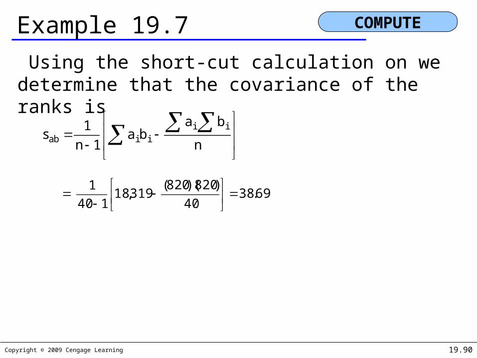
Using the short-cut calculation on we determine that the covariance of the ranks is
COMPUTE
n
baba
1n
1s
iiiiab
69.38
40
)820)(820(319,18
140
1

Copyright © 2009 Cengage Learning 19.91
Example 19.7
The sample variances of the ranks (using the short-cut formula on) are
COMPUTE
n
aa
1n
1s
2
i2i
2a
45.136
40
8205.131,22
140
1 2
n
bb
1n
1s
2
i2i
2b
83.127
40
8205.795,21
140
1 2

Copyright © 2009 Cengage Learning 19.92
Example 19.7 The standard deviations are
Thus,
The value of the test statistic is
p-value = 2P(Z > 1.83) = 2(1 − .9664) = .0672
COMPUTE
68.1145.136ss 2aa
31.1183.127ss 2bb
2929.
)31.11)(68.11(
69.38
ss
sr
ba
abS
83.11402929.1nrz S

Copyright © 2009 Cengage Learning 19.93
Example 19.7
Click Add-Ins, Data Analysis Plus, Correlation (Spearman)
COMPUTE
Copyright © 2009 Cengage Learning 19.94
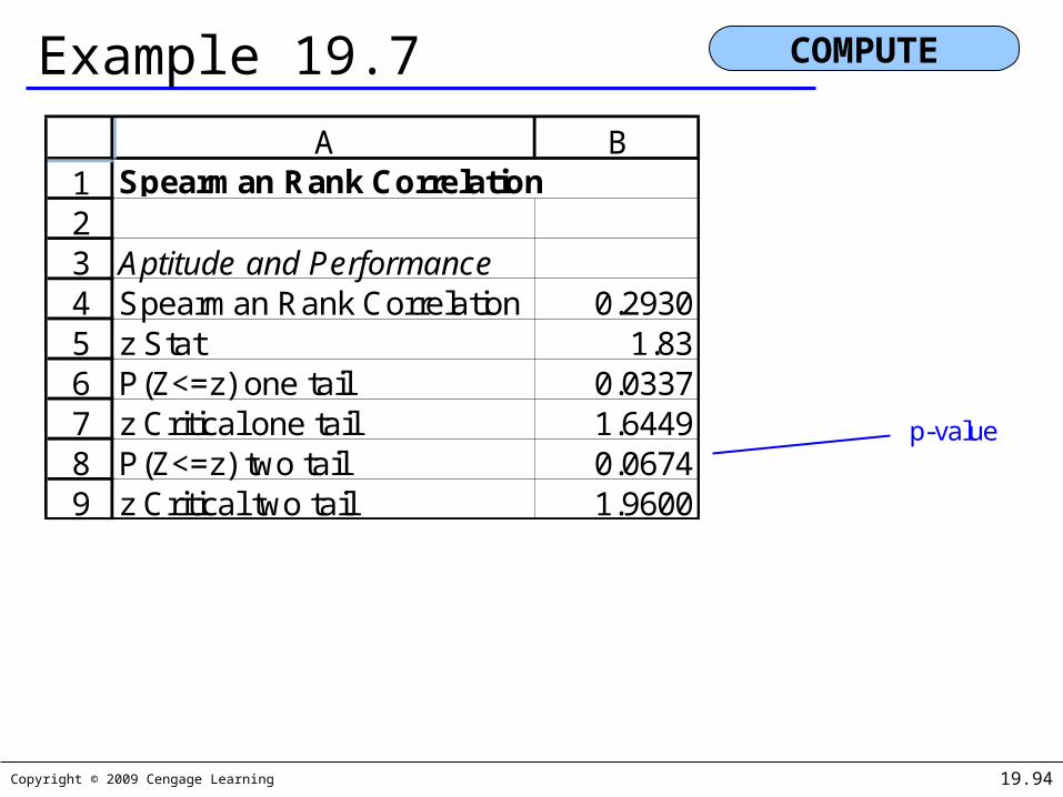
Example 19.7
COMPUTE
123456789
A BSpearman Rank Correlation
Aptitude and PerformanceSpearman Rank Correlation 0.2930z Stat 1.83P(Z<=z) one tail 0.0337z Critical one tail 1.6449P(Z<=z) two tail 0.0674z Critical two tail 1.9600
p-value

Copyright © 2009 Cengage Learning 19.95
Example 19.7
Z = 1.83, p-value = .0674; there is not enough evidence to infer that aptitude test score and performance rating are related.
INTERPRET

Copyright © 2009 Cengage Learning 19.96
Identifying Factors
Factors that Identify the Spearman Rank Correlation Coefficient Test…