Copyright © 1987, by the author(s). All rights reserved...

Copyright © 1987, by the author(s). All rights reserved.

Permission to make digital or hard copies of all or part of this work for personal or

classroom use is granted without fee provided that copies are not made or distributed for profit or commercial advantage and that copies bear this notice and the full citation

on the first page. To copy otherwise, to republish, to post on servers or to redistribute to lists, requires prior specific permission.

NORMAL FORMS FOR NONLINEAR VECTOR

FIELDS—PART II: APPLICATIONS

by

Leon O. Chua and Hiroshi Kokubu

Memorandum No. UCB/ERL M87/82

September 1987


FIELDS—PART II: APPLICATIONS

by

L. O. Chua and H. Kokubu


September 1987

ELECTRONICS RESEARCH LABORATORY

College of EngineeringUniversity of California, Berkeley

94720


FIELDS—PART H: APPLICATIONS

by

L. O. Chua and H. Kokubu


September 1987

ELECTRONICS RESEARCH LABORATORY

College of EngineeringUniversity of California, Berkeley

94720

NORMAL FORMS FOR NONLINEAR VECTOR FIELDS—PART H: APPLICATIONS*

Leon O. Chua and Hiroshi Kokubu''

Abstract

This paper applies the normal form theory for nonlinear vector fields from Part I to several examples of

vector fields whose Jacobian matrix is a typical Jordan form which gives rise to interesting bifurcation behavior.

The normal forms derived from these examples are based on Ushiki's method, which is a refinement of Takens'

method. A comparison of the normal forms derived by Poincare 's method, Tgkens' method, and Ushiki's

method is also given.

For vector fields imbued with some form of symmetry, we impose additional constraints in the normal

form algorithm from Part I in order that the resulting normal form will inherit the same form of symmetry.

The normal forms of a given vector field is then used to derive its versal unfoldings in the form of an n-

parameter family of vector fields. Such unfoldings are powerful tools for analyzing the bifurcation phenomena of

vector fields when the parameter changes. Moreover, since the local bifurcation structure around a highly degen

erate singularity can include some global bifurcation phenomena observed from a less degenerate family of vec

tor fields, it follows that the concepts of normal form and versal unfolding are useful tools for analyzing such

degenerate singularities.

1. INTRODUCTION

In Part I of this paper, we presented a detailed algorithm for deriving the normal forms of smooth vector

fields on Rn. In this paper, this algorithm will be used in several important applications of the normal form

theory. In Section 1, we will derive the well-known normal forms associated with several typical Jordan normal

forms. We will compare our results, which is based on Ushiki's method, with those derived from Poincare* and

Takens' methods. In Section 2, we will investigate some important consequences of symmetry on the normal

forms of vector fields. In the final Section 3, we will apply our results to the versal unfoldings of vector fields

and explore its relationship to Bifurcation theory.

2. EXAMPLES OF NON-DEGENERATE NORMAL FORMS

In this section, we will derive the normal forms associated with the following 3 important Jordan normal

forms:

'This research is supported in part by the Office of Naval Research, Contract N00014-86-K-0351 and theby the National Science Foundation, Grant MIP-8614000.

"L. O. Chua is with the University of California, Berkeley, CA.H. Kokubu is with the Department of Mathematics, Kyoto University, Kyoto, 606, Japan.

0 -1

1 0

0

1

-1

0

0 0

b l o"0 0 l

p 0 0.

(2.1)

(2.2)

(2.3)

Example 2.1. Hopftype

Consider the class of smooth vector fields on R2 which vanish at the origin where the linear part is given

by (2.1); namely, those vector fields having the 1-jet

"--"£+*i (2.4)

on R . To simplify our computation for this example, it is advantageous to introduce the complex coordinates

(2.5)5 = x + iy

%= x-iy

where i = >W. The corresponding differential operators are:

_L 1

JL = ±3? 2

dx dy

JL+i Adx dy

In terms of the new complex coordinate system (£ ,5), the 1-jet in (2.4) assumes the form:

v, = i

(2.6)

(2.7)

(2.8)

(2.9)

Similarly, the following Liebracket formulas in terms of (£ ,^) are useful in the following calculations.

(2.10)**-k*-k+*i =(1-*-/) §*? ±

/

=(i-*-/) {*? ^

=(l-*+/)^A

(2.11)

(2.12)

(2.13)

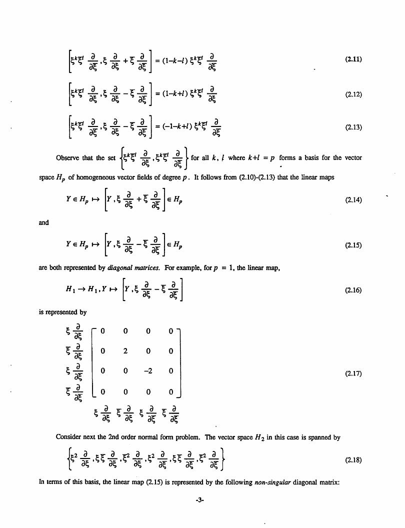
Observe that the set •|̂ *5' 3£* »5*? ~~F [• for all £, / where k+l =p forms a basis for the vector

space Hp of homogeneous vector fields of degree p. It follows from (2.10)-(2.13) that the linear maps

YeHp*-> ett„

and

Y^Hp r+'** *a?

e//r

are both represented by diagonal matrices. For example, for/? = 1, the linear map,

is represented by

d*

*

a?

o

o

-2

0

» a tj- a e a -F- a

5 a^ q 35 * a? q a?

Consider next the 2nd order normal form problem. The vector space H2 in this case is spanned by

{c2 a t^"_a_ ^2 _a_ &2_a_ e^_a_ ^ a5 35 *" 35'9 35'? 35"'" 3?'? 3?

Li terms of this basis, the linear map (2.15) is represented by the following non-singular diagonal matrix:

-3-

(2.14)

(2.15)

(2.16)

(2.17)

(2.18)

-1

1 • O3

-3

O -1

1

Since the image of (2.19) is the whole space H2% dim B2 = 6 where B2 is defined in (5.29) of [1]. It follows

that dim G2 = 0 and the 2nd order components in the normal form is completely eliminated in view of

Theorem 54 from [1].

By repeating the same procedure, we find the linear map (2.15) on H$ is represented by an 8x8 diagonal

matrix, whose diagonal entries are given below with its associated basis component in H3:

-2 0 2 4-4-202

t3 _a_ e2ir _a_ t-£2 _a_ ^ _a_ ±3 a e2v- _a_ *•&, _a_ ^3 _a_s as ss a? ss as s a? s a? s * 35 ss a? s a?

(2.19)

(2.20)

It follows from (2.20) that dim B3 = 6 and hence dim G3 = 2. Let us choose the complementary space G3

spanned by

5? 5 35 q 3? .5?t a __ v- aqai qa?

and consider the following reduced 3rd order normal form problem on G3:

•^«3(') =-%([l'2,V2+g3(0]3]where

v2 = V! = i <£-HfThe (reduced) infinitesimal generator Y2 must satisfy

[Y2,v2]2 = [Y2,vi\2 = 0

that is, y2 = Ki + y2 must satisfy

[y1,v1] = 0 and [y2.vj = 0 -

(2.21)

(2.22)

(2.23)

(2.24)

(2.25)

Since the linear map Y2 —» [Y2l v{\ is non-singular in view of (2.19), we must have Y2 = 0 and hence Y is

of the form

y2 = y, = a* * a?

+ Bt a __•»• aq35 *£

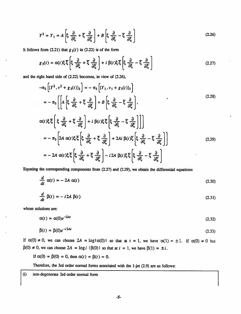
It follows from (2.21) that g3(f ) in (2.22) is of the form

*3(0 = <x(OS? qas qa? + i P(OS?t a _ -r a^35 q3f

and the right hand side of (2.22) becomes, in view of (2.26),

-7C3 [[y2,V2 +*3(0]3] =-7C3 [[Fi.V! +g3(0]3]

= -7C3q a? q a?

+ Be a _ v- a

5 35 93?

o(/)5? 54+5-4 +<P(05?I 35 * 3?

= - K, 24 cc(t)55~

= - 2A cc(OS? ?35 ?3f

e a _ v- a5 35 ?3?

+ 2Ai ml & a _ v- a

5 35 ^35"

- «2A P(f)5? t a __ v- a^35 ^3?

Equating the corresponding components from (2.27) and (2.29), we obtain the differential equations

4- <x(0 =- 2A <x(0dt

-ft p(f) =- ilA p(r)

(2.26)

(227)

(2.28)

(2.29)

(2.30)

(2.31)

whose solutions are:

cc(0 = c^O)*"24' (2.32)

P(0 =me~i2At (2.33)

If a(0) * 0, we can choose 1A = logloc(0)l so that at t = 1, we have cx(l) = ±1. If ce(0) = 0 but

P(0) * 0, we can choose 1A - log/ IP(0) I so that at t = 1, we have p(l) = ±i.

If a(0) = P(0) = 0, then a(0 = p(r) = 0.

Therefore, the 3rdorder normal forms associated with the 1-jet (2.9) are as follows:

(i) non-degenerate 3rd order normal form

±5? ^35 ?3| +.(l +p5? ^K qa?(234)

(ii) degenerate 3rd order normal form (case 1)

'(l ± 5?)t a __ tj- a

q « q a?

(iii) degenerate 3rd order normal form (case 2)

t a _i£- a

* * q a?

In terms of the polar coordinate (r , 6), where

x = r cos 9 , y = r sin 9

a athe vector fields £ rr + £ —— and i k a __ Y- a

qa5 qa?

(2.35)

(2.36)

(2.37)

a acan be identified with the vector fields r —— and -r—

dr 30

respectively. Hence, the normal forms (2.34)-(2.36) simplify further to the following expressions in terms of

(r,9):

(i) non-degenerate 3rd order normal form: ±r3 — + (1+ pr2) —or oQ

(2.38)

(ii) degenerate 3rd order normal form (case 1): (l±r2)—o9

(2.39)

(iii) degenerate 3rd order normal form (case 2): —O0

(2.40)

Using the same procedure, we can of course obtain higher order normal forms. It turns out that for the

non-degenerate case (i), all terms in the normal form beyond the 5th order can be eliminated:

Proposition 2.2

The non-degenerate kth order normal form of vector fields on R with the 1-jet — is given byao

for any k ;> 5

a_dr

(± r2+ocr4)r 4j- +(1 +pr2) -$-d0

(2.41)

This proposition can be proved by induction, similar to that of Proposition 52 from Part I [1]. The proof is

given in the Appendix.

-6-

Example 2.3: Hopf and Zero-interaction type



a ^ a

on R3. The eigenvalues associated with the Jacobian matrix are ±i and 0.

(2.42)

Just as Example 2.1, our calculations are greatly simplified by introducing the complex coordinate

({; ,^, z) in place of (x ,y , z). The simplification is due in part to the following simple formulas

=-(*+o 5*?dz

=(-*+/) 5<f±dz

in addition to (2.10)-(2.13). In terms of the coordinate (|,? ,z), the 1-jet Vj is represented by

vx = it a __-r aq K q a?

(243)

(2.44)

(2.45)

The linear map

YeHp^[YtVl]eHp (2.46)

of the vector space Hp of homogeneous vector fields of degree p has a diagonal matrix representation with

respect to the basis

k*Z*m j^tf?*m -^?VB ~|,* +/+m = (2.47)

For /? = 2, the diagonal entries are given by:

-7-

-1 0

jÂ fy A fJL iz Aa? " dz, ^ b% ^ d% ' 35 as

-3 -1

52 A ^4. â?

2

-2 0

-21 0-1

a v2 _<)_ -p _a_ 2_a_ â? q a? qz a? z a?

-1 1 0

?iî*i pi. fz A z2 As az s az az

Consequendy, the complementary space G2 can be chosen with the basis

{ q * q a? ,zt a __ v- a5 35 ^3? •î-z2i

The reduced 2nd order normal form problem is given by

•^^2(0 =-^2[[yi,v1 +g2(o]2]where Y{ satisfies

[lri,v1] = 0

(2.48)

(2.49)

(2.50)

(2.51)

That is, Yt belongs to the kernel of the linear map Y h> [Y ,v{\ on Hx. Since this linear map is represented

by a diagonal matrix whose diagonal entries are

0 1 -2 0 -1 -1 1 0

t a yr a a * a v- a a * _£_ ^- _a_ _a_q 35 qa^ z 35 ar 3? a? s az * az az

it follows that Y\ is of the form

Y,=A E_3_+?-_3_ + 5e a ^- a5 35 93*~

+czAdz

On the other hand, we can write

82(0 = oc(f)z

»

^3$r a

'3?4

+ f P(0* s a) T a% q a?

+TWK £+*>*£

Substituting (2.53) and (2.54) into the right hand side of (2.50), we obtain

(2.52)

(2.53)

(2.54)

-^(^.v1 +g2(r)]2]=-Ca(02 pA+tA* « 3?

- iC p(Oz

- QA-C) y(t)Z£ ~ -C6(Oz2 -Jjwhere we have made use of the following calculations of the Lie bracket [Y,v]:

t 3 _^- aq as q a?

Y\* Z

5 35 * 3?Z

t 3 t a

35 35". «i •**

5 35 53? 0 0 «i 0

c a t a

q35 q35"0 0 0 0

3

2"37z

* *

eJL+tJL^ J

z ^ £ •'i

(2.55)

Equating the corresponding coefficients in (2.54) and (2.55), we obtain the following 4 linear differential

equations:

d = -Coc (2.56)

p = -cp (2.57)

Y = -(2A-C)y (2.58)

8 = -C5 (2.59)

This implies that, generically, the coefficient y and oneof the coefficients a, p, and 5 can be normalized to ± 1.

Consequently, in terms of the cylindrical coordinate (r ,9,z), the non-degenerate 2nd order normal form can

be chosen to be any one of the following 3 forms:

(a) arz A +(1+pz) A +(Slr2+s2z2) Adr 39 3z

(b) s2rz A+(1+pz) ^ +(Sl r2+5z2} d_

(c) arz A +(i+S22) A +(,ir2+&2) A

(2.60)

(2.61)

(2.62)

where jlt j2 = ±1.

We can repeat the same algorithm to derive higher order normal forms. Here, we will present only the

result of the non-degenerate 3rd order normal form for case (a) of the preceding 2-jets:

(az+az2) r A +(1+pz+fez2) 4? +(sxr2+s2z2+cz3) Aor dd dz

(2.63)

where Sx,s2 = ±1.

Example 2.4: Triple-zero type



a j. a (2.64)

on R3. The eigenvalues associated with the Jacobian matrix consist of 3 zeros.^ Unlike the preceding twoexamples, the linear map

Lp'.YeHp^iY.vJeHp (2.65)

for this example does not have a diagonal matrix representation. We should expect therefore much more tedious

calculations in this example.

Let us examine first the kernel of the linear map

Ll:Hl-^Hl , yhMy.vJ (2.66)

In terms of the basis

dx dx dx dy dy dy dz dz dz

the map Lx is represented by the matrix

0 0 0 1 0 0 0 0 0

-1 0 0 0 1 0 0 0 0

0 -1 0 0 0 1 0 0 0

0 0 0 0 0 0 1 0 0

0 0 0 -1 0 0 0 1 0

0 0 0 0 -1 0 0 0 1

0 0 0 0 0 0 0 0 0

0 0 0 0 0 0 -1 0 0

0 0 0 0 0 0 0 -1 0

Hence, the kernel of L \ is spanned by

•10-

(2.67)

3 3.3 9 ^ d . d

Next, let us choose a basis for H2 as follows:

.2 3•2jL3*

3_3jc

23x

^.^.xz-.r-.yz-z -

j23 3 323 323

v 3^3^'*z^^'*z¥*z¥.2 A

dz dzi-.z2-^-3z ' 3zx~ -^ ,xy -^ ,xz — *y -jT *yz ~ 'z ~

The linear map L2 with respect to the above basis, has the following matrix representation:

0 0 0 0 0 0 1 0 0 0 0 0 > s~"X-2 0 0 0 0 0 0 1 0 0 0 o 1 i( >y

0 -1 0 0 0 0 0 0 1 0 0 0 10 -1 0 0 0 0 0 0 0 1 0 0 ' \\

0 0 -1 -2 0 0 0 0 0 0 1 0 1 v J0 __0__0__0_ -1_ 0 0

0"0

0

0

"00

0

0

0 -*-!-'-~0~"o""6~ 6" 0

/f \ -2 0 0 0 0 0 I 0 1 0 0 0 0

/ \ 0 -1 0 0 0 0 1 0 0 1 0 0 0

I 0 -1 0 0 0 0 0 0 0 1 0 0

\ J 0 0 -1 -2 0 o 1 0 0 0 0 1 0v_y 0 0 0 0 -1 0 J_0 0 0 0 0 1

(r

) (r ^

)

1 o

ll1 o1 °

0

0

-1

-1

0

0

0

0

0

-1

0

0

0

0

-2

0

0

0

0

0

0

0

0

0

0v^-*s V J !° 0 0 0 -1 0

Analyzing the linear map L2, we obtain the following basis for

B2 - images of L2:

xy A>xz A v2 a z d_tz2dtx2±_2xy „dx dx dx dx dx

i a 2 a 32323/% v*xz —,yl — ,yz —-,zl — ,x* — -2xy -r-,ay 3y 3y 3y 3y3 3 2 3 3 2 3

dy dz dz dz dz

dx

3,3z

d_dy

Hence; we can choose the complementary space G2 to B2 in H2 to be the subspace spanned by

•11-

(2.68)

(2.69)

(2.70)

(2.71)

. 2 3 3 3 2 3

Here we must remember that the projection n2:H2-> G2 gives the following:

7C2 •4 = rc23 3 2 3 3 2 3

—5+'2i-

7C23y = *2 *2i-^i+^£ -2**1

and

%3*

2 3 ~ 3 , « 3= 152

=2xz -^- +2y2 A .3z 7 3z

= 2tc2

It follows from (2.67) that a vector field Y\&H\ satisfying,

[r1,v1]=0,

is of the form

3

Y, = Az -%- + Bdx

—+ z —3* 3y

+ C3 3 3

x -?- + y -T" + z -=r3jc 3y

Our 2nd order normal form problem is therefore given by

•|«2(0 =-it2[[r1,v1 +g2(o]2]

=-*2(|Vl.«2(')]]where

g2(0 = «(r) x2 -%- + (3(r) xy -%- + y(t) xz -%-+ 8(f) yl •%-,3_3z

3_3z

d_dz

3z

3_3z

To compute the right hand side of (2.78), it is convenient to derive the following table:

12-

(2.72)

(2.73)

(2.74)

(2.75)

(2.76)

(2.77)

(2.78)

(2.79)

i>-^<^ 2 31 37 *i

a 2 3

3

ZTx3 j. 3 _,. 3

2xz4-~x24-dz dx

3z

3 3 z2 A_xz Adz dx

3

** 3z"

2 3-y Tx

2 3y Tz

Remark 25

3 3Since y — + z — = Vi, we observe that

dx dy yfc+z vVlquendy, there is no need to evaluate any Lie bracket involving y — + z .

dx dy

€ B2 does not affect (2.78). Conse-

3

Using the above table, we evaluate

[Yl9gd=Aa 2xz A-x* a3z 3*

3

+ Ap**-* &

+ i4 y23

2 — XZ

3z 3*_A5V2 a +CctJC2 3

3* 3z

+Cf>xy A+Cyxz A +c8y2Adz dz dz

Therefore, the right hand side of (2.78) becomes

-^([ri.Sd] =-Cax2A-C$xy A_qa a+ Cy)xz A

From (2.75), we obtain

' dxA a%2

Hence,

-C5y2-^- +A an2dz dx

=1A olxz A +2A ay2 4~dz dz

-*2 (l7i .Jd] ="Cax2 A_cp*y A_Cyxz -|-.2 3+ (2A cc-C S)yz -%- ,

3z

(2.80)

(2.81)

(2.82)

(2.83)

Equating the corresponding coefficients of (2.79) and (2.83), we obtain the following 4 linear differential equa

tions:

•13-

d = -C a

p = -cp

y = -Cy

5 = 2Aa-C8

This equation generically gives,

a = ± 1 and 5 = 0,

Hence, the non-degenerate 2nd order normal form is given by:

yi+zi+^2+^xy+yxz)i-where s = ±1.

The differential operator (2.85) can be identified with the differential equation:

x =y

y =z

z = sx2 + $xy + yxz ,

which is equivalent to the following 3rd order differential equation:

x = sx2+ pxc + yxx .

(2.84)

(2.85)

(2.86)

(2.87)

Consider next the 3rd order normal form problem. The basis for the vector space //3 can be chosen as

follows:

* lzm A tXkylzm A iXkylzm J_dx dy dz

*tk + l+m =3

In terms of this basis, the linear map (lexicographic order)

L3:H3^H3;Y3 ^[Yi.vJ

is represented by the 30 x 30 matrix,

A / o

0 A /

0 0 A

where / denotes a 10 x 10 unit matrix, and

•14-

(2.88)

(2.89)

(2.90)

A =

0000000000

-3 000000000

0-100 00 0 0 00

0-2 00000000

00-2-2 000000

0000-100000

000-1000000

0000 -10 -3 000

0 0 0 0 0-10-2 00

00000000-10

It is not difficult to obtain the image 5 3 of the linear map L3 : £3 is spanned by

r

^.

_d_dx

d_dx

d_dx

d_dx

00 a 2 o 30 2dxy -r- yxyz •=- ,xzz — ,yJ — ,yz 2 a 3 adx dx dx

•yd 2 3 id 3 a 2d 3d

3 d „ 2 d 2d- d 20 «x* 3xz y •=- , j:zz —— 2xyz — jcy — + xyz — ,ay

_3_dz

3y dy_adz

3xyz -^f- +y3 — , jc3 — 3x2z — 6xy2 — ,dz

dz

dx dz

dz

2 d 23 n 2 d 2d « 2 d 2d 2d

* ^~XZ Tz'^ T '*z T +2y zT -*> Tx~yz Tz •d.2d 3d *» 2 d 2 d . ,« 2 d

xy2 3T + yz ~r • y t- ~3? zt~ »** t- + 2yz t~dy dz dy dz dz dz

Hence, we can choose the following basis for the complementary space G3:

Hzîîîîî]In order to solve the 3rd order normal form problem

•|«3(0 =-it3([l'2.v2 +j3(r)]3]we must choose the infinitesimal generator Y2 such that

[y2,v2]2 = 0

•15-

(2.91)

(2.92)

(2.93)

(2.94)

(2.95)

that is, we must satisfy

[Yi,v{\ = 0

and

[ri,v2] + [y2,v,]=o

As is discussed on the 2nd order normal form problem, Y^ is of the form,

Yx =Az -§-+Bv1 + Cdx dx dy dz

(2.96)

(2.97)

(2.98)

Hence, Ifi4*0orC*0, then [Yi, v2] does not belong to B2 - Image of L2; in view of (2.81), whereas

I72, Vi] g B2. Therefore (2.96) and (2.97) implies

Yx = constant • vx - K • Vj

Hence, (2.97) becomes

[ri.vj + [IWd = [Kvuv2] + [y2,Vl]

= [Y2-Kv2,v{\ = 0

It follows from (2.100) that

y2 = Kv2 + (kernel of Li).

Here, the kernel of L2 is spanned by

2 3 . 3 , 2 3 « 3 23dx" dx dy dx

Thus we can choose

xz A+yz _a_ +z2±3x ^ 3y 3z

dx '

Y2 =K&^v^ +Az2 A +Bdz

3 ^ 2 3yZ 37 +Z *

+ C ^i^i + £>3 ^ 3 _, 2 3

XZ h VZ + Z3* ^ 3y 3z

On the other hand, from (2.93), g3(t) is of the form

•16-

(2.99)

(2.100)

(2.101)

(2.102)

(2.103)

g3(t) =a(r)x3 -^ +MO*2? -Jj +c(t)x2z A

+d(t)xy2 4- +«('fc>* -I- +/(Oy2z -|- .3z 3z

Observe that

[^2.v2 +̂ (0]3= [Vi,*3(0] +\X1% vj=kvi,^3(o]+ p2 +(kernel), v2J=fevi,$3(Oj +[tfv^vj +[(kernel),v2J .

Since the first term \Kv\ ,g3(t) belongs to £3, it vanishes under the projection %3 :H3 -> G3. The second

term vanishes by itself. Therefore only the third term [(kernel), vj is essential: The Lie bracket [(kernel), v2]

for various kernels and v2 are summarized as follow:

(2.104)

(2.105)

(kernel) ^^^^x*A

dz

3

^-37d

"1Z

-i 2xz2A-1*2*4-dz dx *i-**i 23 a _2xz2±

dz dxa ,a

yzT+z T *» i-* i-** i îî-î-^ d

dy î-vix-î2xz -i-y2 —

dx y dx 4x2z ^--2xy2 A-2** 4-dz dz dx *"£-*£-*>i î-î-î

2 d d 2 adx dy dz

3d 2. d

-* s-* 37 -*£-*•£ 2 3 3-'2 *-** 37

In this table, the following terms belong to B3:

12 o d 3 d 2 d 2. a 23

yz Tz'^Tx'2 Tz'*2 to'**-'* "37Moreover,

2xz2 A _ 2x2z A =2 a2i+^| -2^2 3 +2y2 3

dx dz3z 3x 3z 3z

a „ * a _„„._ 3 ,_._ 32xyz - 2xzz — = 2xyz -^- - 4xyz -^- - 23z 3y 3z 3z

^2 3 __ 33y 3z

= - 2xyz -2- - 23z

^2 JL _ 2xvz —3y ^ dz

-17-

(2.106)

^Tz^Tz-^Tx-^iid 0 2 3 ,= y*z — - 2yzz — +

dz dz

2 3-yzTz~

,2Adx

2 3 , « 2 3xz — + 2y z —dz dz

Ax2zA _2xy2A-2x34-dz dz dx

2 3xz —

3z +2y2zij

j+2y2zi -2

3 ^ 2 3xyzH+yzTz

2 3 2 3*y T~yz Tdx dz

-23 ^ 2 3

xyz^+yz Tz

=4x2z A _2xy2 A „6x2z A _ l2xy2 f- -2dz dz dz dz

x3i_3Ai_^2i3x 3z 3z

=-2x2z -|--14xy2 -|--23z 3z

,31.3,23^213x 3z 3z

2xyz A _v3 A =2xyZA +3xyZA _ yii^zi3z 3z 3z 3z

=$xyzTz~ y3i^i

Za>±-y*z4--2x2*4-dz dz dx

= _4v2 a+2dz

xz2A+2y2zAdz dz

-*£+2 ,z2A+2y2 3dz 3z

_y2z A+4y2 3 _23z dx

-2 x2ZA +2y22 Adx dz

18-

x2z -Z- + 2y2z -r-3x 3z

X dx ^ dy

=_3jc2 a _6^i_dz dz

_,2 a _2^2_3dz dz

,3 a__3x2z^--6xy2^-3x 3z dz

:2y A-x*2A -2xy2-^3y 3z dz

=-4x2z JL-8xy2^L-dz

2 3 3

dz

,3 3__3jc2 3 _6jty2A3z dz 3z

U-A|-2r/ay 3z 3z'

2ax 3

2- a _^ 3 =2;y2 3 _-x z

3x ay dz

2 3 , /, 2 3* z — + 2y*Z —dx dz

2 3+y2"37-

3 2 3

=3^i-A 3 +2y2z 3

dx dz

In all of the above expressions, the terms enclosed by parentheses belong to B3. Hence

-Cs-2xyz£

3^z3xyz^+yzn

_2*2Z a _ Uxy2 Adz dz

-7C3[[r2,V2 +£3(0]3]=-ifc

-cp 5xyzi -Cy 2 3-yzT

-Ds -4jA A - gxy2 Adz dz

-Dpv*

-D y

2z_a

>y2zi

=(2Cs +4Dj)x 2z A +(14C* +8D^)xy2 rr-dz dz

+(2&y - 5C P-Dp)xyz A+ (c y- 3D yly3z '

(2.107)

Finally, equating the corresponding coefficients of (2.104) and (2.107), we obtain the following system of

differential equations,

-19-

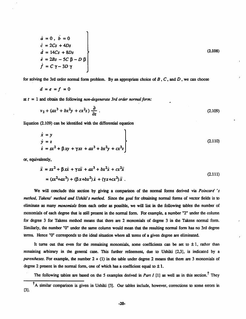
a =0, b =0

c = 2Cs + 4Ds

a* =14Cs +8Dj !• <2-108><?=25^-5Cp-Dp

/ = Cy-3Dy

for solving the 3rd order normal form problem. By an appropriate choice of 5, C, and D, we can choose

d=e=/=0

at t = 1 and obtain the following non-degenerate 3rd order normalform:

v2 +(ax3 +bx^y + cx2z) A .dz

Equation (2.109) can be identified with the differential equation

x =y

y =z

z = sx2 + pxy +yxz + ax3 + fex^ + cx2z

or, equivalently,

x = jx2+ Pxx +yxx +ax3 + bx2x + cx2x

=(sx2-mx3) +(px+6x2)x +(yx+cx2)x .

(2.109)

(2.110)

(2.111)

We will conclude this section by giving a comparison of the normal forms derived via Poincare' 's

method, Tokens' method and Ushiki's method. Since the goal for obtaining normal forms of vector fields is to

eliminate as many monomials firom each order as possible, we will list in the following tables the number of

monomials of each degree that is still present in the normal form. For example, a number "2" under the column

for degree 3 for Takens method means that there are 2 monomials of degree 3 in the Takens normal form.

Similarly, the number "0" under the same column would mean that the resulting normal form has no 3rd degree

terms. Hence "0" corresponds to the ideal situation where all terms of a given degree are eliminated.

It turns out that even for the remaining monomials, some coefficients can be set to ±1, rather than

remaining arbitrary in the general case. This further refinement, due to Ushiki [2,3], is indicated by a

parentheses. For example, the number 2 + (1) in the table under degree 2 means that there are 3 monomials of

degree 2 present in the normal form, one of which has a coefficient equal to ± 1.

tThe following tables are based on the 5 examples derived in Part I [1] as well as in this section. They

[3].rA similar comparison is given in Ushiki [3]. Our tables include, however, corrections to some errors in

-20-

correspond to non-degenerate normal forms firom each example.

Case 1: Simple-zero type in R1 (Example 5.1, Part I)

The Jacobian matrix in this case is a scalar (0)

degree 2nd 3rd 4th 5th 6th 7th

Poincare' 1 1 1 1 1 1

Takens 1 1 1 1 1 1

Ushiki (1) 1 0 0 0 0

Case 2: Hopf type in R2 (Example 2.1)

The Jacobian matrix in this case is:0 -1

1 0

degree 2nd 3rd 4th 5th 6th 7th

Poincare' 0 2 0 2 0 2

Takens 0 2 0 2 0 2

Ushiki 0 1+0 ) o 1 0 0

Case 3: Hopf and Zero-interaction type in R (Example 2.3) in cylindrical coordinate

0 -1

The Jacobian matrix in this case is:1 0

0 o

degree 2nd 3rd 4th 5th

Poincare' 4 6 7 9

Takens 4 6 7 9

Ushiki 2+ (2) 3 9 2

Case 4: Double-zero type in R2 (Example 55, Part I)

The Jacobian matrix in this case is:

Since the linear part in this example is not diagonalizable, Poincarg's method is not applicable.

0 1

0 0

degree 2nd 3rd 4th

Takens

Ushiki

2 2 2

1 + 0) 1 1

•21-

0

Case5: Triple-zero type in R (Example 2.4)

The Jacobian matrix in this case is :

Again, Poincare"s method is not applicable because the linear part is not diagonalizable.

degree 2nd 3rd

Takens

Ushiki

4 6

2 + (l) 3

b i o"0 0 i

p 0 0.

Remarks

1. Both Poincare' and Takens' methods give the same result for vector fields having a diagonalizable linear

part

2. Poincare"s method does not apply, in its original form, to non-diagonalizable vector fields.

3. Takens' method is applicable to all cases.

4. Ushiki's method may be considered as a refinement of Takens' method.

5. Takens' is aware that further refinements are possible and have in fact derived them for cases 1 and 2

[5,6].

6. This paper follows Ushiki's approach since his method gives an explicit algorithm for general vector

fields.

3. NORMAL FORM WITH SYMMETRIES

Many vector fields of practical interest are imbued with some form of symmetry; e.g., reflection symmetry,

point symmetry, rotation symmetry, etc. In such cases, it is natural that their normal forms should exhibit the

same symmetries. Our goal in this section is to show how such additional constraints can be imposed upon the

algorithm and in the preceding section.

Definition 3.1: Vector fields with symmetry

A symmetry, for a vector field v on Rn is a dijfeomorphism y: Rn —> Rn satisfying

(3.1)y v = v

where

y,v(x) £ Dy[fl(x)]'v[r\x)}Example 32:

(3.2)

.22-

Let v be a vector field on R defined by

v(*,y) = (l+y^x2?) .

Then v exhibits a symmetry via the diffeomorphism

y(x,y) = (x,-y),

To see this, we calculate

Dy(x,y) =

and

Y v(x,y) =

1 0

0 -1

1 0

>.-!. y (x,y) = (x,-y)

1 +yi

o -iJL-^.= v(x,y)

(3.3)

(3.4)

(3.5)

(3.6)

It is easy to see that the set of all symmetries for a vector field v forms a group under composition. This

group is called the symmetry group of v. For the above example, the symmetry group contains at least four ele

ments {W,y,8,y ©5}, where 5:(x,y) -» (-x,y), since yoy=8o8 = W and y ° 5 = 5 ° y.

A group made of two elements is firequendy denoted by Z 2. In this section, we shall restrict our con

sideration to vector fields whose symmetry group contains Z2 = {id,y} as a subgroup. To derive a normal

form with symmetry y, we must find appropriate transformations which preserve the same symmetry y, after sub

jecting the vector field to these transformations, as in the preceding section. In other words, the resulting normal

form must also exhibit the symmetry y. Using our notation from [1], our abstract objects in this section consists

of asubspace ySXo of smooth vector fields zXq which vanish at 0and exhibit the symmetry y.

Our next proposition characterizes the class of transformations that preserves symmetry.

Proposition 3.3

Suppose a vector field v exhibits a symmetry y. Then a transformed vector field <|> v also exhibits the

same symmetry y if <J> commutes with y, i.e., y°<|> = § oy, or equivalently,

yo^oy"1 =<]) (3.7)

Proof.

Since y v = v and <J> ©y = yo<|),

Y„G.V> = (Y0^ = (<l>0Y),v = <^(Y,v) = <t>,v (3.8)

Proposition 3.4

-23-

If a local one-parameter group {§'} of transformations is generated by a vector field Y, i.e.,

<J>' = QxptY , (3.9)

then the local one-parameter group

$' = yo<|>' oy1 (3.10)

is generated by y Y.

Proof.

Since <J>' is the flow of the vector field Y,

^<|>'(x) =r(<|>'(x)] * (3.11)holds. Thus,

ft ~*'(X) =ft (Y°*' 0y'1)(X) =Dy (** °Tl(X)) 'ft ** h~1(x))=Dy[(l)/oy-i(x)].y[(|)'(y-^)]

r i r i (3-12)=Dy\rl@Qc))\.Y\rl<y(?))\

=(yj)[tf(x)}.This completes the proof.

•

It follows firom the above propositions that the set

YDiff0 = {$: R" -» R" ,diffeomorphism, $(0) = 0, yo<j> = <j) oy) (3.13)

can be chosen as our transformation group and -fs^o can be chosen as its infinitesimal generators. Once we fixthis transformation group and space, the remaining steps for obtaining the normal form are identical to the

preceding algorithm, as illustrated by the following example.

Example 3.4

Consider vector fields on R1 with a vanishing 1-jet; i.e.,

vi = 0, v(0) = v'(0) = 0 . (3.14)

Let us impose the symmetry

y(x) = -x . (3.15)

The space yS^o can be decomposed into the homogeneous parts

-24-

y ^A-o = y* I 7" 2 ® 7"3 7™ 4 * (3.16)

where each partJtk consists of homogeneous vector fields vk of order k satisfying the symmetry constraint

y0vk=vk, (3.17)

Heiice, for even k, we have

yffjfe = 0 (3.18)

and for odd k, we have

yfY, = Hk . (3.19)

In other words,

Y 0 = #1 © #3 © H5 0 • • • (3.20)

Since we have v2 = 0, our next step is to obtain the simplest 3rd order part; i.e., consider the 3rd order

normal form problem with v2 = 0 under the symmetry y(x) =-x.

The 1-jet v j = 0 implies that the linear map

Lk:^k -*yHk,Yk ->[Yk9vi\ (3.21)

is the zero map for every k. Hence, the complementary space J2k to the image of Lk is simply y/7*, and the

normal form problem is already reduced:

-Jt 8k(0 =- \Yk-1,V*"1 +gk(t)]k (3.22)with

jy*-i 9v*-i J =0,y# Yk~l =Yk~l . (3.23)For k = 3,

Aj3(0 =_[r2^3(o]3 =- [ri .*3<o] (3.24)where

[y2,v2]2 =0 (3.25)

automatically holds for v2 =0. Thus, Y2 need only satisfy y Y2 = Y2; hence Y2 = 0. Defining

Y\ =A* "^ (3.26)and

-25-

i d£3(0 = Ot (Ox3 -r- , (3.27)

we obtain

- [7i.S3<0] =-2Aa(t)x3 (3.28)Equating the coefficients of (3.27) and (3.28), we obtain the differential equation

d = - 24 a . (3.29)

It follows that we can always choose the value of A so that the non-degenerate 3rd order normal form with

symmetry y is given by

v3 = ±x3 — . (3.30)

Similar to Prop. 52 from Part I [1], we can prove that the y-symmetric kth order normal form of vector

fields on R1 with avanishing 1-jet is given by-\

(±x3+ax5) y- aeR. (3.31)

for* ^.5.

Following the same procedure, we have derived the following non-degenerate normal forms with Z 2-

symmetries for several typical examples:

2-dimensional case

(i) non-degenerate 3rd order normal form with the symmetry (x ,y) —> (-x ,-y), whose linear part has

double- zero eigenvalues:

v3 =y -^ +(sx^ax^) — ,s =±1 (3.32)

(ii) non-degenerate 3rd order normal form with the symmetry (x ,y) -» (-x ,y), whose linear part has

double- zero eigenvalues:

v3 =Slxy — + (s^+ay^by3) — , s{ =±1 , s2 =±1 (3.33)

3-dimensional case

(iii) non-degenerate 3rd order normal form with the symmetry (x ,y tz) —» (-x ,-y ,-z), whose linear part

has triple-zeco eigenvalues:

-26-

dx * (334)+ (sx^ax^+bxh+cxyz+dxz2) — , s =±1

dz

(iv) non-degenerate 3rd order normal form with the symmetry (x ty tz) —» (—x ,—y ,z), whose linear part

has triple-zero eigenvalues:

v3 = y -%- + (^xz-^z+fa^+cx^+dfyz2) -£•dx dy

(3.35)

+(j^+ezVz3) -|- , ^! =±1 , s2 =±1dz

(v) non-degenerate 3rd order normal form with the symmetry (x ,y tz) —> (x ,y ,-z), whose linear part has

triple-zero eigenvalues:

v3 =y -^- +(j!X2+axy+to3+cxz2+rfyz2) Adx dy

(3.36)-\

+ (exz+s2z3) — ,s\ =±1 ,j2 =±1dz

4. VERSAL UNFOLDINGS

Our preceding normal form theory consists basically of methods for simplifying ordinary differential equa

tions (ODE) in a neighborhood of their singular points. We have presented various examples of normal forms

having several eigenvalues with a zero real part; namely, multiple zero eigenvalues, or pure imaginary eigen

values, etc. All such eigenvalues which lie on the imaginary axis in the complex plane are called central eigen

values. A singular point of a vector field is said to be hyperbolic if it does not contain any central eigenvalues.

From the Hartman-Grobman theorem, we know that the local phase portraits of vector fields around hyperbolic

singular points are determined by their associated 1-jets, and the center manifold theorem reduces a vector field

with both central and non-central eigenvalues to that with only central eigenvalues. Hence, we will only con

sider vector fields around a singular point where all of its eigenvalues are central.

The above conclusion appears, at first sight, to be rather academic especially from an engineering context

because almost all Jacobian matrices associated with physical systems are hyperbolic; i.e., all eigenvalues have a

non-zero real part. This observation is true only forfixed vector fields. Forfamilies of vector fields, however,

central eigenvalues will always be encountered. In particular, we will show that simple central eigenvalues (i.e.,

multiplicity one) are inevitable in one-parameter families of vector fields, while multiple central eigenvalues are

inevitable in multi-parameter families of vector fields.

Example 4.1

.27-

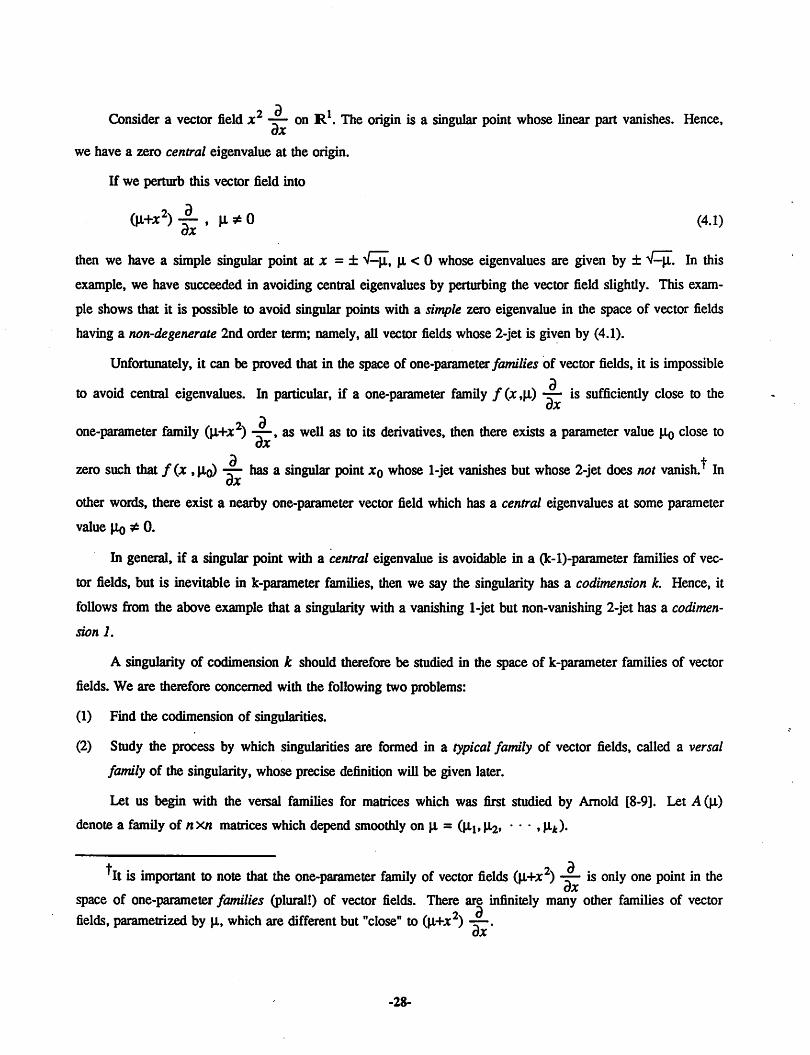
Consider a vector field x2 — on R1. The origin is a singular point whose linear part vanishes. Hence,dx

we have a zero central eigenvalue at the origin.

If we perturb this vector field into

(H+*2) -jj , M- *0 (4.1)then we have a simple singular point at x =±V^T, |x <0 whose eigenvalues are given by ±V^jl. In thisexample, we have succeeded in avoiding central eigenvalues by perturbing the vector field slighdy. This exam

ple shows that it is possible to avoid singular points with a simple zero eigenvalue in the space of vector fields

having a non-degenerate 2nd order term; namely, all vector fields whose 2-jet is given by (4.1).

Unfortunately, it can be proved that in the space of one-parameter families of vector fields, it is impossible

to avoid central eigenvalues. In particular, if a one-parameter family / (x ,{X) — is sufficiently close to thedx

i done-parameter family (\i+x ) —, as well as to its derivatives, then there exists a parameter value \Iq close todx

d tzero such that f(x ,\Iq) — has a singular point x0 whose 1-jet vanishes but whose 2-jet does not vanish.1 In

dx

other words, there exist a nearby one-parameter vector field which has a central eigenvalues at some parameter

value Ho * 0.

In general, if a singular point with a central eigenvalue is avoidable in a (k-l)-parameter families of vec

tor fields, but is inevitable in k-parameter families, then we say the singularity has a codimension k. Hence, it

follows from the above example that a singularity with a vanishing 1-jet but non-vanishing 2-jet has a codimen

sion 1.

A singularity of codimension k should therefore be studied in the space of k-parameter families of vector

fields. We are therefore concerned with the following two problems:

(1) Find the codimension of singularities.

(2) Study the process by which singularities are formed in a typical family of vector fields, called a versal

family of the singularity, whose precise definition will be given later.

Let us begin with the versal families for matrices which was first studied by Arnold [8-9]. Let A (|i)

denote a family of nxn matrices which depend smoothly on ji = CjX|, l^, • • • , \ik).

T tO•It is important to note that the one-parameter family of vector fields (u+x ) -r— is only one point in the

dxspace of one-parameter families (plural!) of vector fields. There are infinitely many other families of vector

fields, parametrized by |1, which are different but "close" to (ll+x2) —.dx

-28-

Definition 42

(i) A family A (p.) is an unfolding of a matrix A0 if A (0) = A0.

(ii) Let A (ji) andA (fL) be unfoldings of a matrix A 0, where ^ and fL need not have the same dimension. We

say A (\i) is induced from A (ft) if there exist an unfolding C(\i) of the identity matrix and a transforma

tion fl = <K|l) satisfying <|)(0) = 0 such that

AOi) =COO •A[<KM)) ' COO"1 (4.2)holds for any \i close to zero,

(iii) An unfolding A (ji.) of A 0 is vewa/ if every unfoldings of A 0 is induced from A (jx).

Example 43

(1) For any 2x2 matrix A0, the family

A(p.) =A0 +H3 JM

is a verca/ family because any unfolding of A 0 can be written as

Ao+ [fa(W t^ft),where fo(0) = 0.

(2) Let A0 denote the 2x2 matrix0 1

0 0. Then the family

0 1

0 0

0 0

Hi H2

is versal becauseany unfolding

0 1

0 0 toft) MX)

is conjugate to the matrix

0 1

0 0

0 0

<fe(l-Hfe) - $^4 (J)! + (j)4

under the transformation

.29-

(4.3)

(4.4)

(4.5)

(4.6)

(4.7)

c =

Remark 4.4

1-Khft) 0

H>iW i(4.8)

The above example shows that the matrix A 0 =

0

0

1

0

0 1

0 0+

Hi H2"H3 H4.

and0 1

0 0+

0 0*Hi H2

•

has at least 2 kinds of versal unfoldings; namely,

(4.9)

Therefore, it is important to obtain versal unfoldings with the minimum number of parameters. Such versal

unfoldings are said to be miniversal.

We will show later that the versal unfolding0 1

0 0

0 0

Hi H2is miniversal.

In order to characterize versal and miniversal unfoldings, we need the following concepts from differential

topology:

Definition 45

(1) Let L be a finite dimensional vector space over R and let X, Y be its subspaces: X, Y <z L. We say

X and Y are transversal (in L) and denote this property by the symbol

X r\Y (inL) (4.10)

if the sum X+K is the whole space L (see Fig. 1). This implies that

dimL <> dim X+dim 7. (4.11)

If the equality holds, then X and Y are said to be minitransversal.

(2) Let M and N be smooth manifolds and let P be a submanifold of N. We say a smooth mapping

f :M —» N is transversal to P at a point x e M if one of the following conditions holds:

(i) f(x)4P

(ii) f(x)=peP and

Df(x) • TXM n TpP in TpN (4.12)

where Df (x) is the tangent map (see Fig. 2)

Df(x):TxM -*Tnx)N .

If Df(x) - TXM and TPP are minitransversal, then we say/ is minitransversal to P atx e M,

-30-

(4.13)

In considering an unfolding A (|i) of A0, we may regard it as a smooth mapping

A :\i -» A (p.)

from the parameter space n to M(n , R).

Our next theorem is fundamental in versal unfoldings.

Theorem 4.6

(4.14)

An unfolding A(\i) of A0e Af(rt ,R) is (mini-)versal if and only if A(\i) is (mini-)transversal to

©(A0) at p. =0,where ©(An) is asubmanifold ofM(n ,R) defined by

©(A0) =^CAoC-Hc e GL(n ,R) (4.15)

Remark 4.7

(1)

(2)

(3)

This theorem is an example of the "versality <=> transversality" principle which originated from the

singularity theory of smooth functions [10]. This principle works for various objects.

If an unfolding A(|l) of A0 is transversal to © (An) at A0, then this type of singularity is inevitable inA (p.); that is, if we slighdy perturb A (\l) to A'(n'), as depicted in Fig. 3, then the family A '(p/) still has

a matrix A0 which is conjugate to A0. If A(jx) is mini-versal, then A(|i) is an unfolding with the least

numberof parameters which contains A n in an inevitable manner. This shows that the numberof parame

ters of a miniversal unfolding is equal to the codimension of A 0 in the spaceM(n , R) of matrices.

This theorem can be easily proved using the inverse function theorem. See [8,9] for the proof.

Corollary 4.7

(1) A miniversal unfolding of the n x n matrix

0 1

An =

is given by

An +

o

Hi • ' H«

(4.16)

(4.17)

(2) A miniversal unfolding of the matrix

-31-

Proof

0 -©o

(On 0

is given by

Hi -<0

where CO is close to C00.

(3) A miniversal unfolding of Aq = 0 is given by

Hn ' • ' Hi«

H«i ' ' ' Vnn

(4.18)

(4.19)

(4.20)

Each statement can be proved by checking the minitransversality of A(ji) to \D(Aq). See [8,9] for the

proof.

We are now ready to consider vector fields.

Definition 4.8

(1) Let Vn be a vector field on R" vanishing at the origin 0. We say a family v(|x) of vector fields on R" is

an unfolding of v0 if v (0) = v0 holds. We do not assume v(|l) vanishes at 0 for fx * 0.

(2) Let v(\i) and w(X) be unfoldings of v0. We say w(X) is induced from v(\i) if there exist a family <J)(A,)

of diffeomorphisms with

<j>(0) = identity (4.21)

anda transformation of parameters \i - \i(X) with

|X(0) = 0 (4.22)

such that

w(X) =̂ )tv[jKX)j (4.23)for X close to zero.

(3) We say an unfolding v(p.) of Vn is k-versal if any unfolding of Vn coincides with an induced unfolding up

to order k.

Remark 4.9

-32-

Instead of coordinate transformations, we may consider the case where v \\l(X) is locally topologicallyequivalent to w(X). (See [8,9] for the definition.) Under this equivalence, v((l) is said to be topologically ver

sal.

Example 4.10

.2x d . _ , ., yd . . .._ ,.. x/„ ^ dAn unfolding (ll+x ) -r- of the vector field x -r- is 2-versal. To prove this, let (t)(x,X) — be anydx dx dx

unfolding of x2 —. Since <|>(x ,0) = x2, ^(0,0) = 2 * 0. Therefore, by the implicit function theorem, thedx

equation <J>x(x A) = 0 can be solved for x as a function of X; namely,

x = T\(X) , with Tl(0) = 0 . - (4.24)

By a family of coordinate transformations,

the vector fields <b(x , X,) -r— can be transformed into the formdx

\|/(X)+X2+ 0(X3) [Adx

(426)

.2, dHence, upon choosing |i = W(X), (426) coincides with (li+x2) — up to order two.dx

The general "versality <=> transversality" principle also works for this case. In particular, by changing

M(n,R)to

>A.q = H j © H2 © © Hk

and ©(An) to

©(v0) = {<!>**v0 I$* e Diff0*} , v0e 9(0* ,

we can prove the following theorem by using the same reasoning as that of Theorem 4.6:

Theorem 4.11

An unfolding v(|X) of v0eyCo is (mini-)k-versal if and only if v is (mini-)transversal to<D(vo) c 9GUm. = o.

Remark 4.12

Note that we restrict the whole space to y(o, not yCk. This means that any unfolding v([i) ofvo€ y^o should vanish at the origin; i.e., v(n)(0) =0. Therefore Theorem 4.11 does not imply Example 4.10

.* dbecause in that case, the unfolding (jx+x^) — does not vanish at O. If we apply this theorem todx

-33-

2 dv0 = x —, we would obtain a 2-versal unfolding

Qix+x2) -2-dx

under the condition that the origin is alway the singular point

(4.27)

Nevertheless, we presented the above theorem because we can easily obtain an unfolding without the

trivial singularity 0 from the k-versal unfolding in 9Cq» an(^ because the following general corollary holds.

Corollary 4.13

Suppose v0e y^o is a non-degenerate kth order normal form with a specified 1-jet Ax —. Then a k-dx

versal unfolding ofv0 in Q(q is obtained upon adding alinear unfolding

<&(u)x — (4.28)

where A + 0(ji) is a versal unfolding of the matrix A. In other words, a versal unfolding of a non-degenerate

normal form can be obtained by adding a linear versal unfolding.

From this corollary, we can obtain the following versal unfoldings automatically:

(i) A =

In polar coordinate:

0 -<D

CO 0 , (CO * 0)

(H ±r2 +otr4) r ^-+ (ofpr2) ^dr d0

(k-versal for any k ^ 5)

(ii) A =0 1

0 0

d P)y — +(^i1x+M.2y±x2+(3xy+ax3) -^~ox dy

(iii) A =

(3-versal)

0 -a)

co 0

0 0

(w*0)

(4.29)

(4.30)

(4.31)

(4.32)

-34-

(Hi+ctz+az2) r -^- +(co+pz+fcz2) -^ +(\L2z+Sir2+s2z2+cz3) — (st =±1)dr 39 9z

(iv) A =

0 1 o"0 0 1

p 0 0.

(3-versal)

y -^- +z -^- + (\Llx+\L2y+\L3z+sx2+$xy+yxz+ax3+bx2y+cx2z) -r- ($ =±1)dx dy oz

(v) A =0 1

0 0

(3-versal)

with the symmetry (x ,y) -»(-x ,-y)

y •§- +(M.1x+^i2y+5x3+ax2y) -£- (s =±1)dx dy

(vi) A =

(3-versal)

0 1

0 0

0 0

with the symmetry (x ,y ,z) -» (-x ,-y ,z)

y -r- +(jXjX+iJ^y+^iXz+ayz+to^x^+fryz2) —dx dy

.2^_2^x_3s 5+ faz+s&'+ez'+fz') -z- (Si = ±1)dz

(3-versal).

(4.33)

(4.34)

(4.35)

(4.36)

The proof of Corollary 4.13 consists of showing the addition of a linear versal unfolding gives a transver

sal family to ©(vn). This is assured by the non-degeneracy assumption since k-jets equivalent to non-

degenerate normal form of order k forms an open set in

H 2 © H 3 © Hi

Due to versal unfoldings, we can study the change in the phase portraits of vector fields near a vector field

with central eigenvalues in a systematic manner. This study constitutes a part of bifurcation theory. Unfor

tunately, since we have only k-versal unfoldings for finite k, our considerations must be restricted to truncated

-35-

vector fields of finite order. Such truncation sometimes gives rise to very complicated and subde problems which

are beyond the scope of this paper. Therefore our descriptions in what follows are incomplete. The reader is

referred to [7,9,11] and the references therein for more details.

Let us begin with the simplest case

-\

(H+*2) -2- on R1 (4.37)dx

which is proved to be 2-versal in Example 4.10. Equation (4.37) is equivalent to the following differential equa

tion:

x = \i + x2. . (4.38)

When the parameter \i changes from a positive to a negative value, the bifurcation behavior of this ODE is

given in the x-space in Fig. 4, or in the (ji ,x)-space in Fig. 5. Such a bifurcation gives birth to a pair of stable

and unstable singular points, and is called a saddle-node bifurcation.

Our next example is given by (4.1). In polar coordinate, (4.1) can be identified with the ODE

} =ohtWV (439)9 = (u+Pr2 , co * 0

Since CO * 0, say CO > 0, we have 6 > 0 for sufficiendy small r. Hence, the local phase portrait near the origin

changes as shown in the (x ,y )-space in Fig. 6, and in the (n ,x ,y )-space in Fig. 7, when we vary the parame

ter |X from a positive to a negative value. Observe that a limit cycle is born from a singular point This oscilla

tion mechanism is called the Hopf Bifurcation.

Remark 4.14

The above arguments are all based on truncated equations. But fortunately, the result is true for any ODE

with a non-degenerate lower order jet More precisely,

(i) For a one-parameter family vQi) of vector fields on R1, if v(|in) can be transformed into the non-

d ddegenerate 2nd order normal form ±x — for some |ln, and if -r— v(|i) & 0, then v(|i) exhibitsdx OH ji =no

the saddle-node bifurcation in a neighborhood of (In.

(ii) Similarly, for a one-parameter family v (\l) on R2, if v (\Iq) can be transformed into the non-degenerate

3rd order normal form

±r3A +(C0+pr2) A fa, *o (4.40)dr dv

in polar coordinate and if ——d[L

v (|X) * 0, then v (|l) exhibits the Hopf bifurcation in a neighborhood

of Ho-

-36-

More complicated bifurcation phenomena can be observed from the family (4.2). Although this family

assumes the origin is a singular point we can eliminate this assumption by making the transformation

x -» x - x0. The resulting family, truncated up to 2nd order, is of the form

y~k +0^2*±*2+tey)^ (4-41)Hence, this is 2-versal. It follows from the result of Bogdanov [12-13] (see also Arnold [9]) that this family

exhibits the 2-parameter bifurcation phenomena shown in Fig. 8. All of the phase portraits in Fig. 8 are shown

near the origin and the parameters Jli, \i2 are also chosen close to zero. This is an example of a local 2-

parameter bifurcation. It is remarkable to observe that, in this bifurcation, both the saddle-node bifurcation and

the Hopf bifurcation are present in addition to a third bifurcation phenomenon whicn yields a homoclinic orbit

Now we can appreciate a fundamental observation from the above local bifurcation theory; namely, a glo

bal bifurcation can be observed from a local bifurcation of a more degenerate singularity. For example,

although a limit cycle can be observed from a vector field with a hyperbolic singular point which requires a

global analysis, the Hopf bifurcation predicts a limit cycle in an arbitrarily small neighborhood of a central

singular point which requires only a local analysis. Similarly, although the bifurcation phenomena in Fig. 9 can

be observed from a 1-parameter family of vector fields, which requires a global analysis, we can observe them

in an arbitrarily small neighborhood of the origin in the above 2-parameter family (4.41), which requires only a

local analysis.

Bifurcations of the other 2-parameter families (4.33) and (4.35) have also been studied in [5], [7], [9],

[14], etc. It remains to consider the bifurcation phenomena in 3-parameterfamilies, such as (4.34), (4.36), etc.

For such families, even strange attractors can be expected to bifurcate locally. Some analytical results, as well

as results based on numerical simulations [4,15], have been reported recendy. However, we are very far from a

complete understanding of these extremely complex phenomena. Part 3 of this paper will therefore be devoted

to this subject

-37-

APPENDIX. PROOF OF PROPOSITION 2.2

Let us begin with the 3-jet

' '-"-i +CHPr^..-* (A.1)

of a vector field v on R , expressed in polar coordinate (r , 8), corresponding to the non-degenerate 3rd order

normal form (2.38). Recall the following useful formulas from (2.12) and (2.13):

pep d e d __ -F- d*s a? ' * ^ ^ a?

=(1-*+/)^ ±

=(-i-k+ntf?-?=a?

(A.2)

(A.3)

Observation (a)

If n = k+l is even, then —k+l is also even and hence ±l—k+l * 0 in (A.2) and (A.3). This implies

that the mapping

Lk:Hk-+Hk ; Y ->[r,vj

is surjective for all even fc; i.e.,

Bjt = Image Lk = Hk , for all even fc (A.5)

Observation (b)

If n = &+/ is odd, then the map L* has a non-empty kernel only for k-l = ± 1.

It follows from Observation (a) that all even order terms in the higher order normal forms are eliminated.

It suffices therefore for us to examine only the odd order terms n = 2m+1, m ;> 1, inductively. For simpli

city, we denote the non-degenerate (2m+l)th order normal form by v(m). Hence, v(1) denotes the 3-jet v3; i.e.,

For m ;> 2, we can choose the complementary space G2m+i to be the subspace spanned by

mr i JL+fJL . <$©•t d _ •£ d* a? q a? (A.6)

Hence, to determine the non-degenerate 5th order normal form v^, the complementary space G5 is

spanned by

\<&& e_L+t_L5 as ?a? . ftff

e d t- d

q as q a?

The corresponding 5th order normal form problem is given by:

•38-

(A.7)

•|s5(0=-H5([lrV+«5(0]5]where Y4 satisfies the constraint

[r4,v3]4 = 0

This implies:

[^i,v1] = 0

[Y2,vi\ = 0

[y3,v1] + [y1,v3]=o

and

[^4.v1] + [r2,v3]=0

It follows from (2.19), (A.10) and (A.11) that

y, =A *as qa? + Bt d _tj- d

and

y, = o

Now, (2.34) and (A. 14) give

Fi.vs] = Yi**&

= 2A s %l + 2Mp(£

t d tt d

5 3$ 5a£"

e d __t- ds a? 5 a?

It follows from (A.12) and (A.16) that A = 0 and Y3e kernel of L3. Hence, we can choose

73-C« e -a_+?-_a_ + d£?t d _ v- d* as q a?

(A.8)

(A.9)

(A.10)

(A.11)

(A.12)

(A.13)

(A.14)

(A.15)

(A.16)

(A.17)

By a similar analysis, (A.13) implies Y4 = 0. Consequendy, the normal form problem (A.8) reduces to:

-jt 8*0 =-%\[Yi,gs(0] +I73,v3]j (A.18)where

-39-

SsO-flCOG©2 5_L+tJLq a^ q a^

Since

we have

Y*=Bk d _tj- d

** qa?= -i5 v

[r1,g5] = i5[g5,v1]=0

+ b(t)(&y

On the other hand,

[r3,v3] = 2(Cp-Ay)(4l)2 t d _ -r d

at" 3f

t d -g- d

q a^ qa?

Equating the corresponding coefficients of (A.19) and (A.22), we obtain the differential equations:

a =0

b =2(Ds-Cp) , s =±1

(A.19)

(A.20)

(A.21)

(A.22)

(A.23)

(A.24)

It follows from (A.23) and (A.24) that a(t) = <z(0), and b(t) = 6(0) + 2(Ds-C p)f. By choosing C = 0,

and an appropriate D, we can always make b(t) = 0 at t = 1. Hence, the resulting 5th order normal form

becomes

Vm = vm + ar —(2) - v(i)dr

=Cs^+arV^- +(1+Pr2) A , , =±1dr d8

Let us consider now the general (2m+l)th order normal form problem on G2m^.\m.

-f *a«.i(t) =-**.+! [[y*" ,va)+«M(o]M]We claim that

82m+i = 0 , m 2l 3

To prove (A.28), consider the following observations:

(i)

-40-

(A.25)

(A.26)

(A.27)

(A.28)

m—\Y2m-l = PC& * as ^ a?

satisfies

[J'2m-l.V(2)]2m=0

Since l^-i6 kernel oiL2m_^%

[Yim.itvi2)}2m =[r2m.1,v1]=0

+ Q(5?)m-1t a _tj- a

•as qa?(A.29)

(A.30)

(A.31)

(ii) The calculation for the Lie bracket [T^-i, v3] for various combinations of Y2m_i and v3 is summarized

below:

^^y>^^ Va12/n-l^^^^ <m-

vsw s a^ s a?

(%\T~X 5 a^ 5a5~

k j

(4-2m)(^m

(2-2m)(S?)m

» *

E-a. +E"-3-V. Jr «

t d Tg- d

5 35 qa?k j

2(55'"t a ^- a5 35 5 35"k

0

J

It follows from observation (i) that we can always choose Y2m_i as the infinitesimal generator; namely,

Hence, the normal form problem (A.27) becomes

-rc^+i [\Y2m-1 >v&) +g2m+iJ2m+1 J

=-K2m+l p2m-l»v3lj

=(2m-4)Ps(Z£T s4-+?t!d% a?

+ {<2m-2)Gs+2Pp}/<59" t d __ v- dqa? 9 a?

Equating the corresponding coefficients of (A.33) and

*2«+l(0 = W)<g©"

we obtain:

qas q a? + i'Y(0<£5"

-41-

e d _ v- dqas q a?

(A.32)

(A.33)

(A.34)

<j> = (2m-4)Ps (AJ5)

\\r = 2P p + (2m-2)Qs (A.36)

Since s * 0 and m > 3, we can always choose an appropriate P and Q at t = 1 so that

<|>(1) = W) = 0 (A.37)

It follows that the (2m+l)th order contribution to the normal form is eliminated for all m > 3. This com

pletes our proof of Proposition 2.2

•42-

FIGURE CAPTIONS

Fig. 1. Subspaces X and Y in this picture are transversal because any point in L can be decomposed into a

point in X and a point in Y. Note that X and Y would not be transversal if they are collinear in this

picture.

Fig. 2. Geometrical interpretation of the transversality of a smooth mapping / between two manifolds M

and N. Here, the manifold M on the left maps into the bold manifold /(M). In particular, x e M

maps top e /(M). Here,/ is transversal because the tangent to/(M) atp intersects the tangent

to the submanifold P at/7 with a finite angle.

Fig. 3. Geometrical interpretation showing the perturbation of an unfolding A (|l) into A '(|i') preserves the

transversality property.

Fig. 4. Phase portraits illustrating the saddle-node bifurcation in the x -space, parametrized by \l.

Fig. 5. Phase portraits illustrating the saddle-node bifurcation in the (n, x)-space.

Fig. 6. Phase portraits illustrating the Hopf Bifurcation on the radial coordinate (on the left) and on the

(x,y)-plane, parametrized by (X. For |i>0 and |i?0, the trajectory is an expanding spiral (r>0 and

6>0). For |I<0, a circular limit cycle with radius r0 is born. All nearby trajectories inside or outside

are repelled from the limit cycle.

Fig. 7. Phase portrait illustrating the Hopf Bifurcation in the ([L,x ,y )-space. Note that each cross section

parallel to the (x,y)-plane on the right Qi>0) or on the (jt,y)-plane (\k=0) itself consists of an

expanding spiral as in Fig. 6. On the other hand, each cross section with the parabola on the left

(jx<0) is a circle, which corresponds to a limit cycle.

Fig. 8. Phase portraits illustrating the 2-parameter bifurcation phenomena associated with the vector field

(4.41).

Fig. 9. Phase portraits exhibiting a global bifurcation producing a homoclinic orbit associated with a 1-

parameter family of vector fields.

-43-

REFERENCES

[1] L. O. Chua and H. Kokubu, "Normal forms for nonlinear vector fields-Part I: Theory and Algorithm."

ERL Memorandum No. UCB/ERL M87/81, University of California, Berkeley, CA 94720, July 1, 1987.

[2] S. Ushiki, "Normal forms for singularities of vector fields," Japan J. Appl. Math., vol. 1,1984, pp. 1-37.

[3] S. Ushiki, "Normal forms for singularities of nonlinear ordinary differential equations," in Computing

Methods in Applied Science and Engineering, VI, Edited by R. Glowinski and J. L. Lions, North Holland,

1984.

[4] S. Ushiki, H. Oka, and H. Kokubu, "Existence d'attracteurs e"tranges dans le deploiement d'une singularity

de'gene'ree d'un champ de vecteurs invariant par translation," C.R. Acad. Sc^ Paris, L 298, Serie I, n° 3,1984, pp. 39-42.

[5] F. Takens, "Normal forms for certain singularities of vector fields," Ann. Inst. Fourier, vol. 23, 1973, pp.

163-195.

[6] F. Takens, "Forced oscillations and bifurcations," Comm. Math. Inst., Rijkuniversiteit, Utrecht, vol. 3,

1974, pp. 1-59.

[7] J. Guckenheimer and P. J. Holmes, Nonlinear Oscillations, Dynamical Systems, and Bifurcations of Vector

Fields, Springer-Verlag, 1983, 2nd Printing, 1986.

[8] V. I. Arnold, "On matrices depending on parameters," Russian Math. Surveys, vol. 26, no.2, 1971, pp.

29-43.

[9] V. I. Arnold, Geometrical Methods in The Theory of Ordinary Differential Equations, Springer-Verlag,

1983.

[10] T. Brocker, Differentiable Germs and Catastrophes, Cambridge University Press, Cambridge, England,

1975.

[11] S. N. Chow and J. K. Hale, Methods of Bifurcation Theory, Springer-Verlag, 1982.

[12] R. I. Bogdanov, "Bifurcation of the limit cycle of a family of plane vector fields," Selecta Math Soviet-

ica, vol. 1, 1981, pp. 373-387.

[13] R. I. Bogdanov, "Versal deformation of a singularity of a vector field on the plane in the case of zero

eigenvalues," Selecta Math. Sovietica, vol. 1, 1981, pp. 389-421.

[14] E. I. Horozov, "Versal deformations of equivalent vector fields for the case of symmetries of order 2 and

3," (in Russian), Trudy Sem. I. G. Petrovskogo, vol. 5, 1979, pp. 163-192.

[15] A. Ameodo, P. H. Coullet, E. A. Spiegel, and C. Tresser, "Asymptotic chaos," Physica 14D, no. 3, 1985,

pp. 327-347.

-44-

Fig.1

M

Fig.2

X-y/^jT

I

x=->/^Fig.5

(i) /i >0

0«

(ii) /x =0

(iii)/*. <0

0*rQss-^

-r

(b)

(c)

Fig.6

(Homoclinic

Bifurcation)

(HopfBifurcation)

(Saddle-node

Bifurcation)

\fjivfjL2)-space

(Saddle-node

Bifurcation)

Fig.8

M<M0(a) (b)

Fig.9

(c)

Copyright © 1987, by the author(s). All rights reserved...

Documents

Transcript of Copyright © 1987, by the author(s). All rights reserved...