The Pennsylvania State University

The Graduate School

Eberly College of Science

COOPERATIVE MAGNETIC RELAXATION IN GEOMETRICALLY

FRUSTRATED RARE-EARTH PYROCHLORES

A Thesis in

Physics

by

Benjamin George Ueland

© 2007 Benjamin George Ueland

Submitted in Partial Fulfillment of the Requirements

for the Degree of

Doctor of Philosophy

May 2007

The thesis of Benjamin George Ueland was reviewed and approved* by the following:

Peter E. Schiffer Professor of Physics Thesis Advisor Chair of Committee

Moses H. W. Chan Evan Pugh Professor of Physics

Ari M. Mizel Assistant Professor of Physics

John V. Badding Associate Professor of Chemistry

Jayanth R. Banavar Professor of Physics Head of the Department of Physics

*Signatures are on file in the Graduate School

iii

ABSTRACT

We report thermodynamic measurements on the cooperative paramagnet

Tb2Ti2O7 and the stuffed spin ices Ho2(HoxTi2-x)O7-x/2 and Dy2(DyxTi2-x)O7-x/2, where 0 ≤

x ≤ 0.67. For Tb2Ti2O7, AC susceptibility data taken down to T = 1.8 K and in applied

magnetic fields up to H = 9 T show the expected saturation maximum in χ(T) and also an

unexpected low frequency dependence (< 1 Hz) of this peak, suggesting very slow spin

relaxations are occurring. Measurements on samples diluted with nonmagnetic Y3+ or

Lu3+ and complementary measurements on pure and diluted Dy2Ti2O7 strongly suggest

that the relaxation is associated with dipolar spin correlations, representing unusual

cooperative behavior in a paramagnetic system.

For the stuffed spin ices Ho2(HoxTi2-x)O7-x/2 and Dy2(DyxTi2-x)O7-x/2, 0 ≤ x ≤ 0.67,

magnetization data show an increasingly antiferromagnetic effective interaction with

increased stuffing x, with Ising like single spin ground states. Although heat capacity

measurements down to T = 0.4 K yield the expected residual entropy for x = 0,

surprisingly, despite the changing magnetic interactions, the total entropy per spin in

(HoxTi2-x)O7-x/2 remains at the spin ice value for all x, while the entropy per spin in

Dy2(DyxTi2-x)O7-x/2 approaches the Ising value of S = Rln2 for x ≥ 0.3. AC susceptibility

measurements confirm different low temperature states in Ho2.67Ti1.33O6.67 and

Dy2.67Ti1.33O6.67, showing a disordered spin freezing in Ho2.67Ti1.33O6.67, and a partial

freezing in Dy2.67Ti1.33O6.67 coexisting with behavior seen in some cooperative

paramagnets and spin liquids.

iv

TABLE OF CONTENTS

LIST OF FIGURES .....................................................................................................vi

ACKNOWLEDGEMENTS.........................................................................................xii

Chapter 1 Introduction and Theory.............................................................................1

1.1 An Overview of this Thesis ............................................................................1 1.2 The Basics of Magnetism for an Experimental Physicist ...............................2 1.3 Magnetic Ordering..........................................................................................5 1.4 Spin Relaxation and the Time Scale of the Measurements ............................8

Chapter 2 Frustrated Systems .....................................................................................14

2.1 Magnetic Frustration.......................................................................................14 2.2 Spin Glasses....................................................................................................15 2.3 Geometrically Frustrated Magnets .................................................................20

Chapter 3 Experimental Techniques...........................................................................25

3.1 Introduction.....................................................................................................25 3.2 Magnetization .................................................................................................25 3.3 AC Magnetic Susceptibility down to T = 1.8 K .............................................29 3.4 Heat Capacity..................................................................................................31 3.5 AC Susceptibility Experiments Performed on a Dilution Refrigerator ..........34

3.5.1 The AC Susceptibility Instrument ........................................................34 3.5.2 The LHe Sample Can and Mounting the Instrument............................38 3.5.3 Performing the Measurements..............................................................42

Chapter 4 Slow Spin Relaxation in the Cooperative Paramagnet Tb2Ti2O7...............45

4.1 Introduction.....................................................................................................45 4.2 Previous Experimental Results .......................................................................46 4.3 Experiment......................................................................................................48 4.4 Results.............................................................................................................49 4.5 Discussion.......................................................................................................54 4.6 Conclusion ......................................................................................................56

Chapter 5 Stuffed Spin Ice..........................................................................................57

5.1 Introduction.....................................................................................................57 5.2 Previous Experimental Results .......................................................................59 5.3 Experiment......................................................................................................61 5.4 Results.............................................................................................................62

v

5.5 Discussion.......................................................................................................76 5.6 Conclusion ......................................................................................................79

Bibliography ................................................................................................................81

Appendix A AC Susceptibility Measurements on a Dilution Refrigerator ................85

A.1 Schematic of the Electrical Circuits Used for AC Susceptibility Measurements................................................................................................85

A.2 Procedure for Converting the Measured Voltage to Susceptibility ...............86

Appendix B Demagnetization Effects ........................................................................89

Appendix C The Van Vleck Susceptibility.................................................................93

Appendix D Data on the Stuffed Pyrochlore Tb2(TbxTi2-x)O7-x/2, 0 ≤ x ≤ 0.67..........95

vi

LIST OF FIGURES

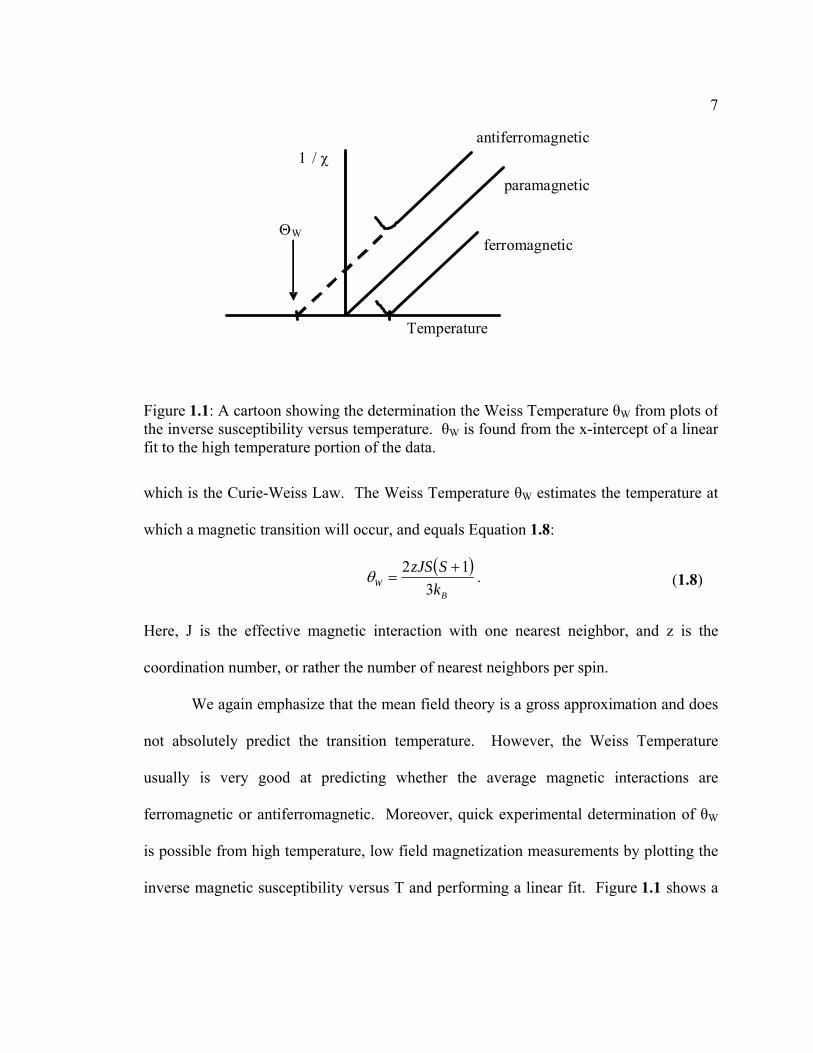
Figure 1.1: A cartoon showing the determination the Weiss Temperature θW from plots of the inverse susceptibility versus temperature. θW is found from the x-intercept of a linear fit to the high temperature portion of the data. .....................7

Figure 1.2: The real and imaginary parts of the complex susceptibility versus the frequency of the applied field. The isothermal and adiabatic susceptibilities occur at the lowest and the highest frequencies, respectively. The phasor representation of the complex susceptibility is also shown. The angle φ is the phase difference between the excitation field and the magnetic response of the sample. ............................................................................................................11

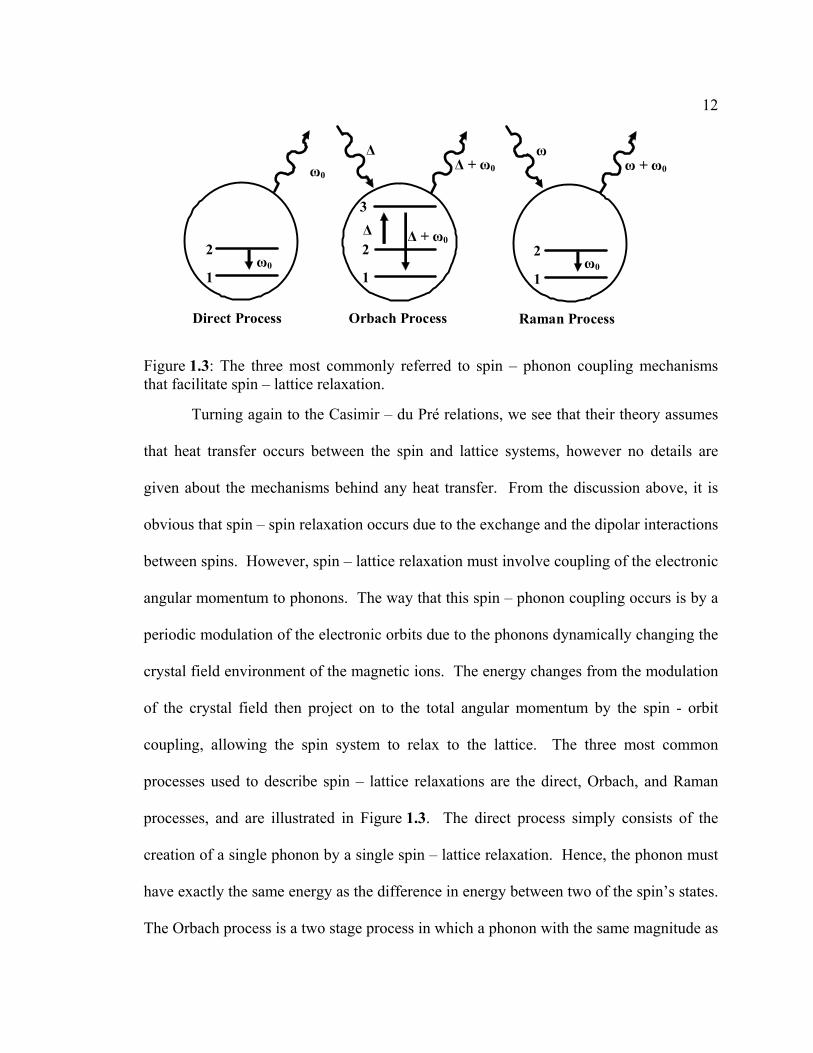
Figure 1.3: The three most commonly referred to spin – phonon coupling mechanisms that facilitate spin – lattice relaxation. .............................................12

Figure 2.1: Schematics illustrating bond disorder (left) and structural disorder (right). Bond disorder refers to a bipartite magnetic interaction having a different nature than the majority of magnetic interactions. Structural disorder means that some lattice sites are different from the majority (i.e. a nonmagnetic lattice is doped with a small percentage of magnetic ions. The disorder in both these examples occurs at random places, giving rise to the second necessary ingredient for a spin glass. .......................................................16

Figure 2.2: Magnetization versus temperature curves at H = 5.9 Oe from experiments on the spin glass CuMn. The percentages in the figure represent the atomic percentage of Mn relative to copper in the alloy. Curves (a) and (c) are from data taken after cooling in the applied magnetic field (FC), while curves (b) and (d) are from measurements made after cooling the material with no applied field (ZFC). This figure is reproduced from Reference [21]. (Copyright 1979 by the American Physical Society.) ..........................................18

Figure 2.3: AC susceptibility data for the spin glass Eu0.2Sr0.8S taken in the absence of a static magnetic field. The oscillating magnetic field was applied with a magnitude of HAC ≈ 0.1 Oe and at various frequencies indicated by the different symbols. The circles represent data taken at f = 10.9 Hz, while the squares represent f = 261 Hz and the triangles represent f = 1969 Hz. The closed symbols show the real part of the susceptibility and the open circles show the imaginary part. This figure is reproduced from Reference [22]. (Copyright 1983 by the American Physical Society.) ..........................................19

Figure 2.4: An illustration of geometric frustration of a magnetic lattice. For ferromagnetic (FM) interactions, all three spins can simultaneously satisfy

vii

their nearest neighbor interactions. For antiferromagnetic interactions (AFM), only two spins can simultaneously minimize their energy......................21

Figure 2.5: Examples of various possible geometrically frustrated magnetic lattices, labeled with their corresponding three dimensional space groups. The two drawings at the top illustrate two dimensional frustrating lattice geometries, while the bottom drawings depict three dimensional frustrated lattice geometries. This figure is reproduced from Reference [15]. (Copyright 1996 by Gordon & Breach.)...............................................................22

Figure 2.6: Unpublished magnetization data showing inverse DC susceptibility versus temperature of the geometrically frustrated magnet Ba2Sn2ZnGa4Cr6O22, at H = 50 Oe. The line shows a linear fit to the high temperature data, which yielded the values for θW and p in the Curie-Weiss law. Ba2Sn2ZnGa4Cr6O22 is a Q-S ferrite, in which the magnetic Cr ions form kagome layers. .............................................................................................23

Figure 3.1: A schematic of the pickup coils in a Quantum Design, Inc. Magnetic Property Measurement System. The superconducting coils are arranged in a second order gradiometer configuration, meaning that the outer two coils are wound in one direction and the inner two coils are wound in the opposite direction. The sample is attached to a rod that is pulled through the coils by a motor located at the top of the cryostat. The illustration is of longitudinal pickup coils, which means that the magnetic moment is measured along the direction of the magnetic field. .............................................................................28

Figure 3.2: A schematic of the AC Magnetic Susceptibility Option for the Quantum Design, Inc. Physical Property Measurement System reproduced from the instruction manual [33]. (Copyright 2000 by Quantum Design, Inc.)..30

Figure 3.3: A schematic of the sample puck used with the Heat Capacity option of a Quantum Design, Inc., PPMS. The left side of the figure shows a top view of the sample platform. The four wires are soldered on the bottom of the platform to a heater and a resistor (shown as dashed lines). The right side shows a side view of the platform, meant to illustrate that it is suspended by the wires over a hole going straight through the sample puck. (Some artistic license has been taken in the drawing of these schematics.) ................................33

Figure 3.4: The LHe sample can used to perform AC susceptibility experiments on a He3/He4 dilution refrigerator. The picture on the left shows the entire sample can attached to the dilution refrigerator, and the pictures on the right show top and side views of the bottom half of the sample can. All of the pictures have different scales................................................................................39

viii

Figure 3.5: A picture and schematic of the AC susceptibility coil set mounted on the dilution refrigerator.........................................................................................41

Figure 4.1: The network of corner sharing tetrahedra in the pyrochlore lattice formed by the magnetic Tb3+ cations in Tb2Ti2O7. This figure is reproduced from Reference [37]. (Copyright 1999 by the American Physical Society.).......47

Figure 4.2: The real and imaginary parts of the AC susceptibility of Tb2Ti2O7 for various frequencies at applied fields of H = 0, 5, and 9 T. This figure is reproduced from Reference[28]. (Copyright 2006 by the American Physical Society.) ................................................................................................................50

Figure 4.3: The magnetic susceptibility of Tb2Ti2O7 at H = 5 T. The top panel includes low frequency AC measurements from the MPMS, higher frequency measurements from the PPMS at higher frequency, and [dM/dH]dc obtained from magnetization data, as described in the text. The bottom panel shows the measured magnetization M(T) at various magnetic fields used to determine [dM/dH]dc (H increases from bottom to top). A high degree of polarization can be seen in M(T) at the fields where slow relaxation is occurring. This figure is reproduced from Reference[28]. (Copyright 2006 by the American Physical Society.)......................................................................52

Figure 4.4: Comparison of the ac magnetic susceptibility at f = 10 Hz and [dM/dH]dc for both (TbxM1-x)2Ti2O7 and (DyxM1-x)2Ti2O7, as described in the text. Note that the dependence is virtually eliminated for the highly dilute samples. The dip in the H = 0 AC data of the diluted Dy samples is a consequence of simple single-ion relaxation studied previously, which unlike the frequency dependence we observe, follows an Arrhenius law [30]. This figure is reproduced from Reference [28]. (Copyright 2006 by the American Physical Society.) .................................................................................................53

Figure 5.1: The local ordering of the H+ in ice (left) and the local ordering of the spins in spin ice (right). ........................................................................................60

Figure 5.2: The percentage of A-sites on the A2B2O7 pyrochlore lattice containing Ti4+, as more Ho or Dy is stuffed into the lattice (lines are guides to the eye). The drawing within the graph illustrates the effect of stuffing on the A and B-sites of the pyrochlore lattice, in which the circled B-site has its Ti replaced by a lanthanide. Parts of this figure are reproduced from Reference [64]. (Copyright 2006 by Nature Publishing Group.) ...................................................63

Figure 5.3: (a) The Weiss temperature and saturation magnetization (T = 2 K, H = 5.5-7 T) plotted versus x for the various Ho2(HoxTi2-x)O7-x/2 samples. The Weiss temperature was determined from fits to the Curie-Weiss law; the estimated uncertainty in the magnetization is ±5% based on the uncertainty in

ix

sample mass. (b) The inverse dc magnetic susceptibility versus temperature for x = 0 and 0.67. The lines are fits to the data used to determine θW, as described in the text; the effective moment p obtained from these fits is within 2% of the accepted value for Ho. This figure is reproduced from Reference [64]. (Copyright 2006 by Nature Publishing Group.) ........................65

Figure 5.4: Magnetization data for Dy2(DyxTi2-x)O7-x/2, 0 ≤ x ≤ 0.67. (a) The Weiss Temperature θW as a function of stuffing x was obtained from fits to data taken in a field of H = 0.1 T. Examples of the fits are shown in (b). (c) M(H) at T = 2 K for each value of x.....................................................................66

Figure 5.5: (a) The total specific heat of Ho2(HoxTi2-x)O7-x/2 for x = 0, 0.3 and 0.67 at H = 0 and 1 T. The dashed and solid lines represent the lattice and nuclear contributions, as described in the text. (b) The total magnetic entropy (integrated from below T = 1 K to T = 22 K) as a function of x at H = 0 and 1 T. The blue and black dashed lines represent the predicted ice entropy and total spin entropy values, respectively. (c) The temperature dependence of the integrated entropy for the limiting compositions, at H = 0 and 1 T. This figure is reproduced from Reference [64]. (Copyright 2006 by Nature Publishing Group.)................................................................................................67

Figure 5.6: (left) The specific heat of Dy2(DyxTi2-x)O7-x/2, x = 0, 0.3, 0.67, at H = 0. The inset shows the H = 0 magnetic entropy obtained by integrating the specific heat from at least T = 0.5 K, after subtracting out scaled specific heat data on nonmagnetic Lu2(LuxTi2-x)O7-x/2, x = 0, 0.3, 0.67, (shown as dashed lines in the main graph). (right) The total magnetic entropy of Dy2(DyxTi2-

x)O7-x/2, 0 ≤ x ≤ 0.67, at H = 0, 1 T, and 1.5 T. The solid line shows the corresponding total entropy for Ho2(HoxTi2-x)O7-x/2 at H = 0...............................69

Figure 5.7: The real and imaginary parts of the H = 0 AC susceptibility versus temperature of Ho2.67Ti1.33O6.67 for various measurement frequencies. Data above T > 2 K was taken with the ACMS, while data taken below T = 2 K was taken in the dilution refrigerator. The inset shows the imaginary part of the susceptibility taken from dilution refrigerator measurements. .......................70

Figure 5.8: The real and imaginary parts of the H = 0 AC susceptibility versus temperature of Dy2.67Ti1.33O6.67 for various measurement frequencies. Data above T > 2 K was taken with the ACMS, while data taken below T = 2 K was taken in the dilution refrigerator. The inset shows the imaginary part of the susceptibility taken from dilution refrigerator measurements. .......................72

Figure 5.9: The field dependence of the real part of the AC susceptibility versus temperature of Dy2.67Ti1.33O6.67 for various measurement frequencies. Each panel shows data taken at a different applied magnetic field (H = 0 – 2 T, from left to right). .................................................................................................73

x

Figure 5.10: The f = 50 Hz AC susceptibility versus applied DC field of Ho2.67Ti1.33O6.67, at various temperatures. Data were taken at T = 0.3 K and T = 1.8 K while sweeping the field at rates of 0.01 T/min and 0.1 T/min, respectively. The inset shows M(H) for T ≤ 1.8 K, determined by integrating χ′(H)......................................................................................................................74

Figure 5.11: The f = 50 Hz AC susceptibility versus applied DC field of Dy2.67Ti1.33O6.67, at various temperatures. Data was taken while sweeping the field at a rate of 10 Oe/min. The inset shows M(H) for T ≤ 1.8 K, determined by integrating χ′(H). Note the log scale on the inset’s vertical axis....................75

Figure A.1: The electrical circuits used to measure the AC susceptibility as described in Section 3.12.3. For most of the measurements, the secondaries were connected to a preamplifier located before the secondary lock-in amplifier. All experimental connections between the dilution refrigerator and external instruments were made using coaxial cables with BNC connectors. The resistances used in the primary circuit were R1 = 48.2 Ω and R2 = 1.085 kΩ, and the ground for the primary circuit was taken at the shield of the BNC connector supplying the AC voltage. The reference phase for the secondary lock-in was taken between one of the R2 resistors and the primary circuit’s ground. ..................................................................................................................85

Figure B.1: A cartoon of the demagnetization effect for an ellipsoid with uniform magnetization M lying along an external field H. The polarization of the ellipsoid creates magnetic poles at either end of the sample, which in turn create an effective internal field [H' - H]. .............................................................90

Figure D.1: The Weiss temperature θW and effective moment p as a function of stuffing x in Tb2(TbxTi2-x)O7-x/2. The parameters were obtained from fits on H = 0.1 T magnetization data to the Curie Weiss law, over T = 7 – 14 K. (These data were taken by M.L. Dahlberg.) .........................................................95

Figure D.2: Magnetization versus field data on Tb2.67Ti1.33O6.67 at T = 2 K. (These data were taken by M.L. Dahlberg.) .........................................................96

Figure D.3: The magnetic specific heat versus temperature of Tb2(TbxTi2-x)O7-x/2 at H = 0 and 1 T. All data were taken upon cooling in the applied magnetic field. Lattice contributions were subtracted out by scaling to data on non-magnetic Lu2(LuxTi2-x)O7-x/2, x = 0, 0.3, and 0.67. (Hyperfine contributions should not become important until below T = 400 mK [31].)..............................97

Figure D.4: The magnetic specific heat divided by temperature versus temperature of Tb2(TbxTi2-x)O7-x/2 at H = 0. Lattice contributions were subtracted out by scaling to data on non-magnetic Lu2(LuxTi2-x)O7-x/2, x = 0, 0.3, and 0.67.

xi

(Hyperfine contributions should not become important until below T = 400 mK [31].) ..............................................................................................................98

Figure D.5: The magnetic specific heat divided by temperature versus temperature of Tb2(TbxTi2-x)O7-x/2 at H = 1 T (field cooled). Lattice contributions were subtracted out by scaling to data on non-magnetic Lu2(LuxTi2-x)O7-x/2, x = 0, 0.3, and 0.67. (Hyperfine contributions should not become important until below T = 400 mK [31].)......................................................................................99

Figure D.6: The integrated magnetic entropy versus temperature of Tb2(TbxTi2-

x)O7-x/2 at H = 0. Lattice contributions were subtracted out by scaling to data on non-magnetic Lu2(LuxTi2-x)O7-x/2, x = 0, 0.3, and 0.67. ..................................100

Figure D.7: The integrated magnetic entropy versus temperature of Tb2(TbxTi2-

x)O7-x/2 at H = 1 T (field cooled). Lattice contributions were subtracted out by scaling to data on non-magnetic Lu2(LuxTi2-x)O7-x/2, x = 0, 0.3, and 0.67. .....101

Figure D.8: The real part of the H = 0 AC susceptibility of Tb2.67Ti1.33O6.67 versus temperature for various measurement frequencies. Open symbols represent data taken in the ACMS, while closed circles represent data taken in the dilution refrigerator. These data were calibrated assuming χ′(H = 5 T, T = 1.8 K) = 0 (see Section 3.5.3). ..............................................................................102

Figure D.9: The real part of the f = 50 Hz AC susceptibility of Tb2.67Ti1.33O6.67 versus field at various temperatures, and field sweeping rates. These data were calibrated assuming χ′(H = 5 T, T = 1.8 K) = 0 (see Section 3.5.3)............103

Figure D.10: The real part of the f = 50 Hz AC susceptibility of Tb2.67Ti1.33O6.67 versus field at T = 0.3 K and 0.2 K, taken after initially zero field cooling or field cooling the sample. These data were calibrated assuming χ′(H = 5 T, T = 1.8 K) = 0 (see Section 3.5.3)............................................................................104

xii

ACKNOWLEDGEMENTS

I am indebted to a great many people who have helped and supported me while

completing this work. Foremost, I thank my advisor Peter Schiffer for his invaluable

friendship, assistance, and advice over the past six years. I can not imagine having a

better advisor, and it has been a privilege to know and work with him.

I also thank my family and friends for all of their support, especially my parents,

Stephen and Carol. They have always been there when I needed them, and they have

done everything possible for me to succeed in life.

Chapter 1

Introduction and Theory

1.1 An Overview of this Thesis

Magnetism is widely exploited in contemporary technologies. From simple

compasses, to electrical generators, to computers, magnetism literally powers the world.

The practical applications of magnetism all stem from research into the basic properties

of magnetism and magnetic materials, and new research into magnetic systems continues

to provide us with new technology, and, most importantly, advances our knowledge of

the physical world.

This thesis reports low temperature thermodynamic experiments on two systems

of geometrically frustrated magnets: the cooperative paramagnet Tb2Ti2O7 and the stuffed

spin ice Ln2(Ti1-xLnx)O7-x/2, where Ln = Ho or Dy and x = 0 – 0.67. This first chapter

gives an overview of some basic theory describing the thermodynamic properties of

magnets, while chapter two discusses magnetic frustration and presents data illustrating

basic features of frustrated magnetic systems. Next, chapter three describes the

experimental techniques used in this work. We then move on in chapters four to

recounting previous results for Tb2Ti2O7 and present our experimental results and

conclusions. Chapter five follows in a similar manner, with a discussion on the stuffed

spin ices.

2

1.2 The Basics of Magnetism for an Experimental Physicist

Magnetic materials contain ions with magnetic moments, meaning that these ions

respond to a magnetic field. This work is chiefly concerned with electronic magnetic

moments created by the total angular momentum of an electron, which in general consists

of both the orbital and spin angular momentum. The orbital angular momentum arises

from the electron’s periodic motion around a nucleus, while spin angular momentum is

an intrinsic property of electrons (and certain other particles) that can be derived from

relativistic considerations. Colloquially, the total magnetic moment of a particle is

referred to as its spin. Thus, magnetic materials contain spins that can interact with

external magnetic fields and with other spins in the material.

Magnetic interactions fall into four basic groups: paramagnetism, diamagnetism,

ferromagnetism, and antiferromagnetism. Paramagnetism is the property of an ion or

material to align to an applied magnetic field, while diamagnetism is the property of an

ion or a material to counteract an applied field. Ferromagnetism and antiferromagnetism

refer to spins aligning either parallel or opposite to their neighboring spins, which can

lead to collective behavior of the spins in the material.

Diamagnetic behavior results from Lenz’s Law, which tells us that for a current

loop enclosing a magnetic field, any change in the magnetic flux through the loop will

create a current in the loop opposing the change in flux. Hence, the orbital motion of

electrons around a nucleus causes all atoms to show some degree of diamagnetism in

response to a change in any external field. Hence, even insulating materials with no open

shells exhibit diamagnetism. Additionally, perhaps the best known examples of

3

diamagnetic behavior have been made when applying magnetic fields to superconductors,

where demonstrations such as a magnet levitating over a piece of superconducting

material are well known.

As stated above, paramagnets easily align their spins to an applied magnetic field.

Considering a system of N free spins in an applied field, we can describe the system as a

canonical ensemble with a partition function given by Equation 1.1:

where µi is the magnetic moment of ion i, and β is the Boltzman constant kB times the

system’s temperature T [1][2]. We define the magnetic moment in the j direction in

Equation 1.2:

Here, gjk is the Landé g-factor (or spectroscopic splitting factor), Sk is the total angular

momentum of a single ion, µB is the Bohr magneton, and j and k represent spatial

directions [3]. Equation 1.2 uses the Einstein summation convention, meaning that we

must take the sum over the repeated index k.

From the partition function in Equation 1.1, we can derive the thermal averages of

all the macroscopic properties of the spin system. For example, we can find the average

magnetization M of the system by taking the derivative of the natural logarithm of the

partition function with respect to the field and dividing by -β. With proper normalization,

this yields the average component of M along H, which is proportional to the Brillioun

function as shown in Equation 1.3:

∑=i

HieZ βμ , (1.1)

Bkjkj Sg μμ = . (1.2)

4

For small fields (H << T), we can expand M as a power series in H, yielding Curie’s

Law, Equation 1.4:

This law predicts a T-1 dependence of the susceptibility at high T and small H, which has

been confirmed experimentally. Also, one can define the effect moment by Equation 1.5:

and determine the value from simple fits to experimental data. The effective moment is

important in determining whether or not spins will act as free spins or whether some

correlation between spins is occurring. It also gives clues about the effect of the

crystalline electric field on the spins, since the crystal field should partially lift the

degeneracy of the angular momentum multiplet of each spin. Thus, the correct value

used for S must correspond to the total angular momentum of the crystal field level an

electron is in at a given temperature. In the case of some transition metals, the crystal

field is strong enough to quench the orbital angular momentum, meaning that only the

spin angular momentum will be the valid quantity to use in Equation 1.5 when analyzing

experimental results.

⎥⎦

⎤⎢⎣

⎡⎟⎠⎞

⎜⎝⎛−⎟

⎠⎞

⎜⎝⎛ ++

= βμβμμ gSHSS

gSHS

SS

SgSNM BBB 21coth

21

212coth

212 . (1.3)

TkSSgN

HM

B

B

3)1(22 +

==μχ . (1.4)

)1(2 += SSgp , (1.5)

5

1.3 Magnetic Ordering

Magnetic ordering due to spin-spin interactions occurs when the interactions are

strong enough to dominate the other energies present in the system. As stated above,

ferromagnetic or antiferromagnetic interactions can exist between neighboring spins.

Ferromagnetic interactions occur when the lowest interaction energy between the spins

occurs when they align parallel to each other, while antiferromagnetic interactions occur

when the spins obtain their lowest interaction energy by pointing opposite to each other.

Magnetic interactions between spins are primarily due to the magnetic dipole field

set up by each spin and quantum mechanical exchange, with exchange typically being the

more predominant of the two. The dipole energy simply comes from treating a spin as a

magnetic dipole, yielding an energy decreasing with distance as r-3 that depends greatly

on the magnitude of the spin. While the exchange interactions result from quantum

mechanical considerations of the indistinguishable nature of electrons. In other words, if

one considers two H atoms brought close enough together, the electronic wave functions

of each atom will mix, making it impossible to assign a specific electron to a specific

nucleus. In general, the exchange of electrons between two nuclei will bond atoms

together. However, the electrons must follow the Pauli Exclusion Principle, and their

atomic states are also subject to the Stark splitting of the crystalline electric field. These

restrictions on the exchange of electrons between ions can give rise to magnetic ordering.

Since exchange interactions are due to orbital mixing, they are generally short

range, but in most cases, they are stronger and more influential than any dipolar spin-spin

interactions present. In addition, the exchange interaction does not need to be direct,

6

meaning that a nonmagnetic intermediate ion can exist between two magnetic ions and

share electrons with both. This situation is termed superexchange. Other types of

exchange interactions exist, and the interested reader can find their descriptions in a solid

state or magnetism textbook [3][4][5][6].

Even though exchange involves the overlap of electronic wave functions, we can

often write the exchange Hamiltonian for spin i quite simply as Equation 1.6:

where Jij is the exchange constant representing the exchange interaction between spin i

and spin j. The negative sign implies that if Jij is positive, the lowest interaction energy

between the spins is ferromagnetic. Similarly, if the exchange constant is negative, then

antiferromagnetic interactions exist.

Since the summation in Equation 1.6 is over all the spins in the material, we

cannot exactly solve for the exchange energy. However, we can reasonably approximate

the energy with the mean field approximation, in which we truncate the sum over j to

being a sum only over the first nearest neighbors to spin i. This method interprets the

interactions on spin i by its j nearest neighbors as an effective magnetic field on spin i.

Surprisingly, this rather gross approximation sometimes yields results that agree rather

well with experimental data. In fact, adding the mean field energy into Equation 1.1,

determining the magnetization, and expanding as before yeilds Equation 1.7:

∑−=j

jiiji SSJH 2 , (1.6)

( )WB

B

TkSSgNθ

μχ−

+=

3)1(22

, (1.7)

7

which is the Curie-Weiss Law. The Weiss Temperature θW estimates the temperature at

which a magnetic transition will occur, and equals Equation 1.8:

Here, J is the effective magnetic interaction with one nearest neighbor, and z is the

coordination number, or rather the number of nearest neighbors per spin.

We again emphasize that the mean field theory is a gross approximation and does

not absolutely predict the transition temperature. However, the Weiss Temperature

usually is very good at predicting whether the average magnetic interactions are

ferromagnetic or antiferromagnetic. Moreover, quick experimental determination of θW

is possible from high temperature, low field magnetization measurements by plotting the

inverse magnetic susceptibility versus T and performing a linear fit. Figure 1.1 shows a

ΘW

1 / χ

Temperature

paramagnetic

ferromagnetic

antiferromagnetic

Figure 1.1: A cartoon showing the determination the Weiss Temperature θW from plots of the inverse susceptibility versus temperature. θW is found from the x-intercept of a linear fit to the high temperature portion of the data.

( )B

W kSzJS

312 +

=θ . (1.8)

8

cartoon illustrating the determination of θW from the x-intercept of the fit. Note, that the

slope of the linear fit also allows determination of the effective moment per spin.

1.4 Spin Relaxation and the Time Scale of the Measurements

A spin relaxes when it aligns with an external field due to the torque created by

the interaction between the spin and field. For a thermodynamical system of N identical,

non-interacting (or very weakly interacting) spins, the response of the magnetization of

the system to a static (DC) magnetic field is Equation 1.9:

If the direction of the field is taken as the z – direction, then the equilibrium

magnetization M0 will also be in the z – direction. However, if we apply an additional

field along the z – direction that is strong enough to create a different macroscopic state,

then once we remove this additional field, the system must relax back to its original

equilibrium, which will require some finite length of time. If we apply the additional

field periodically at a frequency corresponding to a length of time quicker than the

relaxation time of the spin system, then the spins will remain in a non-equilibrium state.

Measurements made on the system at the same frequency as the perturbing field will then

yield a magnetization less than M0. Quantitatively, adding a small sinusoidal perturbing

field H1 to Equation 1.9 results in the well known Bloch equations [7]. For the case

above, the Bloch equations reduce to Equation 1.10:

HSgdt

dMB ×−= μ . (1.9)

1

10 cos)(T

mtHHMgdt

dm zzB

z −+×=

ωχμ , (1.10)

9

where χ0 is the static susceptibility, ω is the frequency of the perturbing field, T1 is the

longitudinal relaxation time of the system, and mz is the component of the magnetization

in the z – direction [3]. Note that Equation 1.10 is actually an approximation, since only

the static susceptibility is present.

By its derivation, the Curie-Weiss Law deals with spins in thermal equilibrium, or

in other words, it tells us the static or DC susceptibility χDC of a material. The law is

valid when χDC equals the isothermal susceptibility χT, which is the susceptibility when

the spins and, for our purposes, the lattice in which they are imbedded are at the same

temperature. If we assume that the spins and the lattice are two separate

thermodynamical systems able to transfer energy between each other by spin-phonon

coupling, than an adiabatic susceptibility χS can be defined as the susceptibility when no

heat is exchanged between the spin and lattice systems. The importance in the difference

between these two limiting susceptibilities and how spin freezing is defined becomes

apparent once the time over which a measurement becomes comparable to the relaxation

time of the spin system. One way we can realize such a measurement is by performing

AC susceptibility experiments, in which we apply to the material a small field with a

sinusoidally varying magnitude with time in addition to any other external field. The

dynamics of this technique are discussed above and are governed by Equation 1.10 if the

measurement is performed with longitudinal fields. AC susceptibility experiments are

usually carried out over a relatively low frequency range from 0.01 Hz < f < 10,000 Hz.

Higher frequency ranges can be investigated using techniques such as electron

paramagnetic resonance EPR [8], muon spin resonance µSR [9], or neutron

scattering[10]. We emphasize again that in all these dynamic experiments, we effectively

10

make measurements at the same frequency as the perturbing probe. Therefore, we are

able to see non-equilibrium dynamics and must recognize whether the spins are

completely freezing, or if they are just relaxing fast too slowly to be observed by the

experiment.

We can make a quantitative interpretation of the difference between the

isothermal and adiabatic susceptibilities by using the Casimir - du Pré relations [11]

given in Equations 1.11 and 1.12:

These equations consider χ to be a complex quantity, with a real part χ' that is in

phase with an external field oscillating of angular frequency ω, and an imaginary part χ''

that is 90° out of phase with the field. The spin lattice relaxation time is given by τ1. It

should be pointed out that these relations assume that the time rate of change of heat

flowing from the spin system to the lattice is directly proportional to the difference in

temperatures of the spin and lattice systems. In addition, one could derive these two

equations from Equation 1.10, where it will than be obvious that T1 is the same as the

spin – lattice relaxation time τ1. Figure 1.2 gives a graphical representation of the

relations and shows the phasor representation of χ. Note that χ'' is much smaller than χ'

and peaks as χ' rapidly decreases. In addition, to the Casimir - du Pré relations, the

components of χ must also follow the Kramers - Kronig relations [12][13].

The assumption that the lattice and spins are two separate thermodynamic systems

is valid when there are large differences in time scales between spin - spin and spin -

21

21 τωχχ

χχ+

−+=′ ST

S (1.11)

( )21

21

1 τωωτχχ

χ+−

=′′ ST . (1.12)

11

lattice relaxation. This is typically the case at low temperatures, where the spin-spin

relaxation time can be many orders of magnitude higher than the spin-lattice relaxation

time. The large difference in the relaxation times relates to the density of states of each

system and to the amount that their energies overlap. Additionally, the lattice only

directly affects the orbital angular momentum, since the spin angular momentum exists in

a different space, and the spin angular momentum only interacts with the lattice through

the spin – orbit coupling. Thus, the spin angular momentum is usually well separated

from the lattice phonons, allowing spin - spin relaxation to occur independent of any spin

– lattice relaxation [14].

10-3 10-2 10-1 100 101 102 1030

0.5

1.0χ = χ′ + iχ′′

φχ

χ′′

χ′

χ′′

χ′

χS

χ / χ

0

ωτ1

χT

Figure 1.2: The real and imaginary parts of the complex susceptibility versus thefrequency of the applied field. The isothermal and adiabatic susceptibilities occur at thelowest and the highest frequencies, respectively. The phasor representation of thecomplex susceptibility is also shown. The angle φ is the phase difference between the excitation field and the magnetic response of the sample.

12

Turning again to the Casimir – du Pré relations, we see that their theory assumes

that heat transfer occurs between the spin and lattice systems, however no details are

given about the mechanisms behind any heat transfer. From the discussion above, it is

obvious that spin – spin relaxation occurs due to the exchange and the dipolar interactions

between spins. However, spin – lattice relaxation must involve coupling of the electronic

angular momentum to phonons. The way that this spin – phonon coupling occurs is by a

periodic modulation of the electronic orbits due to the phonons dynamically changing the

crystal field environment of the magnetic ions. The energy changes from the modulation

of the crystal field then project on to the total angular momentum by the spin - orbit

coupling, allowing the spin system to relax to the lattice. The three most common

processes used to describe spin – lattice relaxations are the direct, Orbach, and Raman

processes, and are illustrated in Figure 1.3. The direct process simply consists of the

creation of a single phonon by a single spin – lattice relaxation. Hence, the phonon must

have exactly the same energy as the difference in energy between two of the spin’s states.

The Orbach process is a two stage process in which a phonon with the same magnitude as

1

2 ω0

ω0

Direct Process

ω + ω0

Raman Process

ω

1

2 ω0

Δ + ω0

Orbach Process

Δ

3

1

2 Δ + ω0

Δ

Figure 1.3: The three most commonly referred to spin – phonon coupling mechanisms that facilitate spin – lattice relaxation.

13

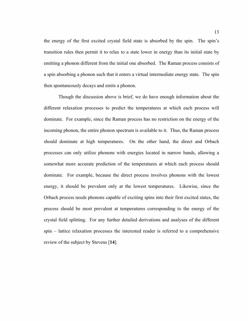
the energy of the first excited crystal field state is absorbed by the spin. The spin’s

transition rules then permit it to relax to a state lower in energy than its initial state by

emitting a phonon different from the initial one absorbed. The Raman process consists of

a spin absorbing a phonon such that it enters a virtual intermediate energy state. The spin

then spontaneously decays and emits a phonon.

Though the discussion above is brief, we do have enough information about the

different relaxation processes to predict the temperatures at which each process will

dominate. For example, since the Raman process has no restriction on the energy of the

incoming phonon, the entire phonon spectrum is available to it. Thus, the Raman process

should dominate at high temperatures. On the other hand, the direct and Orbach

processes can only utilize phonons with energies located in narrow bands, allowing a

somewhat more accurate prediction of the temperatures at which each process should

dominate. For example, because the direct process involves phonons with the lowest

energy, it should be prevalent only at the lowest temperatures. Likewise, since the

Orbach process needs phonons capable of exciting spins into their first excited states, the

process should be most prevalent at temperatures corresponding to the energy of the

crystal field splitting. For any further detailed derivations and analyses of the different

spin – lattice relaxation processes the interested reader is referred to a comprehensive

review of the subject by Stevens [14].

Chapter 2

Frustrated Systems

2.1 Magnetic Frustration

Common sense suggests that every physical system should be capable of finding

some single ground energy state - a macroscopic state with the lowest overall energy.

The Third Law of Thermodynamics quantifies this supposition by requiring that the

entropy of a system go to zero as the temperature approaches zero [1][2]. In a classical

sense, this means that once there is not enough heat, or other energy, present in a closed

thermodynamic system to excite its constituents out of their individual ground energy

states, a single macroscopic ground state for the entire system should form. However,

observations show that some thermodynamical systems apparently have several

macroscopic states possessing its expected ground state energy. Such systems are said to

have multiple degenerate macroscopic ground states, meaning that even at T = 0 it is

possible for the system to switch between different states. If the degenerate ground states

arise from an inability to simultaneously minimize all interactions between the particles

in the system, then the system can be classified as being frustrated.

This dissertation concerns Geometrically Frustrated Magnets (GFM), which are

magnetic systems unable to reach a single ground energy state, due to the relative

locations of their magnetic moments on a regular crystal lattice [16][17][18][19]. In

other words, the frustration arises from an incompatibility between the geometry of the

15

spin arrangement and the local spin-spin interactions, resulting in the formation of many

degenerate macroscopic ground states. It is important to note that other types of

magnetic frustration occur. For example, a class of materials called spin glass exists,

which also contain frustrated magnetic interactions. Since studies on spin glasses under

the context of frustration started long before studies on many now recognized GFM, it is

valuable to compare experimental results on GFM to results on spin glasses.

2.2 Spin Glasses

Spin glasses must contain two basic properties: disorder (or randomness) and

frustration. Disorder refers to spins not being located at distinct positions on a lattice

(structural disorder), or it can mean that the magnetic interactions between spins are not

all the same and do not occur in a regular, periodic fashion (bond disorder). Figure 2.1

contains two cartoons illustrating the differences between bond and structural disorder in

a spin glass. The disorder in the magnet then causes frustration, meaning that frustration

alone is not enough to create a spin glass. More examples of disorder and frustration in

spin glasses can be found in Mydosh’s comprehensive text on spin glasses [20].

16

We can view the energy topology of a spin glass as numerous local energy

minima separated by many different large energy barriers, which impede relaxation

between the different minima. Thus, the barriers obstruct the formation of a macroscopic

ground state, resulting in a number of nearly energy equivalent macroscopic ground

states. As a result, a spin glass exists in a metastable state, since its constituents

seemingly can not overcome the large energy barriers and form a global ground state. In

actuality, the many large energy barriers cause the spin glass to relax into lower energy

states over extremely long time scales (>>100 s) and with a large distribution of

relaxation times. For comparison, a typical ferromagnet in a conventional long range

ordered state without different magnetic domains would relax into its ground state with a

much narrower distribution of relaxation times.

Despite their slow spin relaxation, spin glasses have a number of magnetic

experimental signatures. However, they share many of these signatures with other

magnetic systems, meaning that experiments showing evidence for glassiness do not

FM

FM

FM

AFM

Bond Disorder Structural Disorder

FM

FM

FM

AFM

FM

FM

FM

AFM

Bond Disorder Structural Disorder

Figure 2.1: Schematics illustrating bond disorder (left) and structural disorder (right). Bond disorder refers to a bipartite magnetic interaction having a different nature than themajority of magnetic interactions. Structural disorder means that some lattice sites aredifferent from the majority (i.e. a nonmagnetic lattice is doped with a small percentage of magnetic ions. The disorder in both these examples occurs at random places, giving riseto the second necessary ingredient for a spin glass.

17

necessarily indicate that the measured material is a spin glass. It is therefore important to

perform a variety of experiments on a material with glassy properties before labeling it as

a spin glass, especially if the material’s structure is well ordered. As will be discussed

further below, a number of similarities exist between experimental data for spin glasses

and geometrically frustrated magnets. As such, we next discuss some experiments valid

for both types of systems. The discussion below will mainly focus on results for spin

glasses, and we will reserve comparison of these results to data taken on geometrically

frustrated magnets for the next section.

Perhaps the hallmark experiment to perform on a spin glass, is to make two

measurements of the magnetization M as a function of temperature at very low fields (H

~ 0.01 T) - first after initially cooling the material in zero applied magnetic field (ZFC)

and then after initially cooling the sample in the measurement field (FC). Since the spin

glass exists in a metastable state, we will see a bifurcation in the resulting M(T) data at

the glass temperature created by the different initial states of the ZFC and FC

measurements. Figure 2.2 shows an example of this phenomenon. The ZFC

magnetization curves have a lower magnitude below the glass temperature due to both

the self averaging of the spins while cooling and the slow relaxation times of the spins

after applying field. In fact, if we perform a ZFC magnetization experiment on a spin

glass by measuring M as a function of time at a temperature below the glass transition,

then once we apply the field M will slowly change from M = 0 to the value that would

have been obtained if we had used the FC procedure. The time over which this will

happen, though, can be paraphrased from Mydosh’s book as being, “[greater than] the

average lifetime of a graduate student [which] is only about 108 s [20].”

18

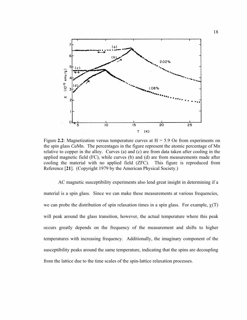
AC magnetic susceptibility experiments also lend great insight in determining if a

material is a spin glass. Since we can make these measurements at various frequencies,

we can probe the distribution of spin relaxation times in a spin glass. For example, χ(T)

will peak around the glass transition, however, the actual temperature where this peak

occurs greatly depends on the frequency of the measurement and shifts to higher

temperatures with increasing frequency. Additionally, the imaginary component of the

susceptibility peaks around the same temperature, indicating that the spins are decoupling

from the lattice due to the time scales of the spin-lattice relaxation processes.

Figure 2.2: Magnetization versus temperature curves at H = 5.9 Oe from experiments onthe spin glass CuMn. The percentages in the figure represent the atomic percentage of Mnrelative to copper in the alloy. Curves (a) and (c) are from data taken after cooling in theapplied magnetic field (FC), while curves (b) and (d) are from measurements made after cooling the material with no applied field (ZFC). This figure is reproduced fromReference [21]. (Copyright 1979 by the American Physical Society.)

19

This indicates that the spins are absorbing energy from the oscillating field. Figure 2.3

shows AC susceptibility data on the spin glass Eu0.2Sr0.8S taken at H = 0 and HAC ≈ 0.1

Oe. Different symbols represent different measurement frequencies, as described in the

figure caption. Although not shown in this figure, application of even a static magnetic

field as small as H ~ 0.01 T can be sufficient to disturb the spin glass state. In AC

susceptibility measurements, the peak in χ′(T) will decrease in magnitude and broaden in

temperature as the field is increased. Also, the temperature of the maximum will

Figure 2.3: AC susceptibility data for the spin glass Eu0.2Sr0.8S taken in the absence of a static magnetic field. The oscillating magnetic field was applied with a magnitude ofHAC ≈ 0.1 Oe and at various frequencies indicated by the different symbols. The circlesrepresent data taken at f = 10.9 Hz, while the squares represent f = 261 Hz and thetriangles represent f = 1969 Hz. The closed symbols show the real part of thesusceptibility and the open circles show the imaginary part. This figure is reproducedfrom Reference [22]. (Copyright 1983 by the American Physical Society.)

20

decrease in accordance with either the de Almeida-Thouless line (for an Ising spin glass

in a field) or the Gabay-Toulouse line (for transverse spin freezing with weak

irreversibility in a non-Ising spin glass) [20][23][24]. The fact that such a small external

field can affect the spin glass is surprising, since the effective temperature of the applied

field is often orders of magnitude smaller than the glass temperature.

2.3 Geometrically Frustrated Magnets

This dissertation is chiefly concerned with Geometrically Frustrated Magnets

(GFM), in which the regular arrangement of the spins on a crystal lattice creates

frustration. Figure 2.4 shows a simple gedankenexperiment illustrating geometrical

frustration. We perform the experiment by imagining an equilateral triangle with Ising

spins located at its vertices. The spins are constrained to the plane of the page and

allowed to point either up or down. If we now turn on effective ferromagnetic (FM)

interactions between the spins, we see that all three spins can simultaneously minimize

their bipartite interactions by pointing in the same direction. However, if we turn on

antiferromagnetic (AFM) interactions between the spins, then only two of the three

interactions can be simultaneously satisfied, resulting in frustration. For the AFM Ising

triangle, there are six different spin configurations with the lowest energies, meaning that

there are six global ground states, as compared to the two global ground states in the

ferromagnetic triangle. Thus, if this situation is repeated an infinite number of times, the

spins will form a lattice of side sharing triangles with antiferromagnetic nearest neighbor

interactions, and there will be no single well defined macroscopic ground state.

21

It is important to note that Ising spins are not necessary for a geometrically

frustrated system. In fact, a large degree of frustration exits on the pyrochlore lattice

when 3-D AFM Heisenberg spins are located at the corners of corner sharing tetrahedra.

Figure 2.5 shows various geometrically frustrated magnetic lattices. The triangle and

kagome lattices are two dimensional, while the face-centered cubic, pyrochlore, and

garnet lattices are three dimensional. It is interesting, but not surprising, that all of these

lattices contain triangular arrangements of spins: the triangular lattice consisting of side

sharing triangles, the garnet and kagome lattices consisting of corner sharing triangles,

and the FCC lattice consisting of side sharing tetrahedra. The pyrochlore lattice is

comprised of spins forming corner sharing tetrahedra, and materials with its structure are

the focus of this thesis.

The many degenerate ground states available to a frustrated magnet can create a

situation in which the spins are free to fluctuate, at temperatures well below the

equivalent temperature of their nearest-neighbor interactions. This means that like spin

FM FM

FM

AFM AFM

AFM

FRUSTRATED

FM FM

FM

AFM AFM

AFM

FRUSTRATED

Figure 2.4: An illustration of geometric frustration of a magnetic lattice. Forferromagnetic (FM) interactions, all three spins can simultaneously satisfy their nearestneighbor interactions. For antiferromagnetic interactions (AFM), only two spins cansimultaneously minimize their energy.

22

glasses, magnetization versus temperature measurements are key to the initial

characterization of the material. Specifically, if we fit low field (H < 0.1 T), high

temperature (T ~ 102 K) M(T) measurements on a GFM to the Curie-Weiss law

(Equation 1.7) and determine the value of the Weiss temperature θW (Equation 1.8), we

will see that M(T) follows the Curie-Weiss law down to temperatures well below θW.

Figure 2.6 shows an example of a Curie-Weiss fit on unpublished χ-1(T) data for the

GFM Ba2Sn2ZnGa4Cr6O22 (published data for this material can be found in References

[25] and [26]). The line represents a linear fit to the data at T > 100 K, and the Weiss

temperature and effective moment (Equation 1.5) obtained from the fit are indicated.

Figure 2.5: Examples of various possible geometrically frustrated magnetic lattices,labeled with their corresponding three dimensional space groups. The two drawings atthe top illustrate two dimensional frustrating lattice geometries, while the bottomdrawings depict three dimensional frustrated lattice geometries. This figure is reproducedfrom Reference [15]. (Copyright 1996 by Gordon & Breach.)

23

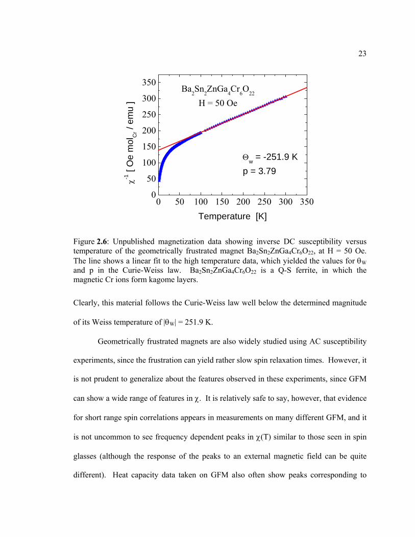
Clearly, this material follows the Curie-Weiss law well below the determined magnitude

of its Weiss temperature of |θW| = 251.9 K.

Geometrically frustrated magnets are also widely studied using AC susceptibility

experiments, since the frustration can yield rather slow spin relaxation times. However, it

is not prudent to generalize about the features observed in these experiments, since GFM

can show a wide range of features in χ. It is relatively safe to say, however, that evidence

for short range spin correlations appears in measurements on many different GFM, and it

is not uncommon to see frequency dependent peaks in χ(T) similar to those seen in spin

glasses (although the response of the peaks to an external magnetic field can be quite

different). Heat capacity data taken on GFM also often show peaks corresponding to

0 50 100 150 200 250 300 3500

50

100

150

200

250

300

350

Θw = -251.9 Kp = 3.79

Ba2Sn2ZnGa4Cr6O22

H = 50 Oe

χ-1 [

Oe

mol

Cr /

emu

]

Temperature [K]

Figure 2.6: Unpublished magnetization data showing inverse DC susceptibility versus temperature of the geometrically frustrated magnet Ba2Sn2ZnGa4Cr6O22, at H = 50 Oe. The line shows a linear fit to the high temperature data, which yielded the values for θWand p in the Curie-Weiss law. Ba2Sn2ZnGa4Cr6O22 is a Q-S ferrite, in which the magnetic Cr ions form kagome layers.

24

short range spin correlations. Some example AC susceptibility and specific heat data can

be found in References [27][28][29][30][31][32].

We also should not overlook that much work exists examining faster spin

relaxations in geometrically frustrated magnets. Specifically, neutron scattering and

muon spin resonance experiments can tell a great deal about the local correlations

between spins and the nature of any magnetic ordering that may be present.

Chapter 3

Experimental Techniques

3.1 Introduction

Various experiments were used to determine the magnetic properties of the

materials studied for this dissertation. This chapter gives descriptions of these

measurement techniques, which included magnetization, AC magnetic susceptibility, and

heat capacity experiments. We performed all of these experiments in commercially

available equipment manufactured by Quantum Design, Inc. [33], and, additionally, we

performed AC susceptibility experiments down to T = 60 mK using a custom made

instrument thermally anchored to the mixing chamber of a He3/He4 dilution refrigerator.

3.2 Magnetization

As previously discussed, the bulk magnetic response of a material a long time

after changing external parameters to the system (i.e. magnetic field, temperature,

pressure…) is the static (DC) magnetization M of the material. For this work, we

performed magnetization measurements using a Quantum Design, Inc., Magnetic

Property Measurement System (MPMS). The system’s main components consist of an

insulated liquid He dewar, a long cylindrical insert (probe), a control cabinet, a rotary

vane vacuum pump, and a desktop computer. The probe contains the sample chamber,

impedance, cooling valves, electrical heaters, and measurement circuits. It sits at the

26

center of the dewar, submerged in liquid He, and a superconducting magnet surrounding

the sample chamber can apply persistent fields up to H = 7 T with a uniformity of 0.01%

over the length the measurement. Control of the sample chamber temperature is made by

regulating the flow of liquid/gaseous He into the cooling annulus using automated valves

and electrical heaters. In this way, the temperature of the sample chamber can be

precisely varied between T = 1.8 K – 400 K at rates from 10-3 – 101 K / s and kept stable

within ± 0.5%. The sample chamber is kept in vacuum (~ 0.001 Torr), and samples are

inserted into it through an airlock that can be purged with He from the bath.

We generally will mount a sample in a clear plastic drinking straw inside of a

gelatin capsule. Since most of the materials measured were powders, the small magnetic

susceptibility of the gelatin capsule provided a convenient means to contain the sample.

The powder did not fill the volume of the capsule, so cotton was packed on top of the

powder to keep it at the bottom of the capsule. We then position the gelatin capsule at

the center of the straw and tie it into place with clear Nylon thread. Since we measured

materials containing large spins, the magnetic background from the straw, thread, cotton,

and capsule was at most two orders of magnitude smaller than the measured moment of

the sample, the background due to the sample mounting technique could be safely

neglected.

We would then take the straw and connect its top to the end of a long thin rod

using a combination of Kapton and masking tapes. The rod consisted of two pieces, a top

piece made from thin walled stainless steel tubing, and a smaller length of non-magnetic

thin walled brass tubing. (The straw was attached to the brass section of the rod.) When

inserted into the sample chamber, the top of the rod was anchored to a stepper motor that

27

moved the rod vertically. A light coat of vacuum grease on the rod and a sliding seal at

the top of the airlock allow vertical movement of the rod while keeping the sample

chamber under vacuum.

To perform magnetization measurements, the MPMS uses a superconducting

quantum interference device SQUID inductively coupled to a tank circuit. A

measurement is made by smoothly pulling a small sample (<0.1 cm3) through four loops

of wire, while a DC magnetic field is applied. The wire loops are configured to form a ≈

3 cm long second order gradiometer, meaning that the top and bottom loops are wound in

one direction, while the two middle loops are wound in the opposite direction (i.e. if the

top and bottom loops are wound clockwise, then the two middle loops would be wound

counter-clockwise). The coil set is designed to reject the uniform field created by the

magnet to within 0.1%, making the detector insensitive to any drift in the magnetic field.

A schematic of the pickup loops is shown in Figure 3.1. By Faraday’s Law, the change

in magnetic flux created by pulling the magnetic sample through the wire loops will

induce a voltage in the loops as in Equation 3.1:

Here, E is the induced electric motive force (EMF), φm is the magnetic flux, t is time, and

the negative sign is due to Lenz’s Law. The EMF causes an electric potential, so E has

units of Volts.

The EMF induced by the sample’s magnetic moment creates a current that is then

inductively coupled through a transformer to the SQUID circuit. The current induced by

the sample changes the magnetic flux in the SQUID circuit, and a feedback circuit then

dtd

E mφ−= . (3.1)

28

acts to counteract the change of flux by producing an opposing magnetic field. The

current the feedback circuit creates is fed across a resistor, and the voltage across the

resistor is recorded, providing an accurate measurement of the sample’s magnetic

moment. This procedure allows the instrument to determine changes as small as 10-7

emu (1 emu = 1 electromagnetic unit = 1 erg/G) of the moment in the sample chamber as

the sample rod is extracted.

Magnetic Field

Sample

Figure 3.1: A schematic of the pickup coils in a Quantum Design, Inc. MagneticProperty Measurement System. The superconducting coils are arranged in a secondorder gradiometer configuration, meaning that the outer two coils are wound in onedirection and the inner two coils are wound in the opposite direction. The sample isattached to a rod that is pulled through the coils by a motor located at the top of thecryostat. The illustration is of longitudinal pickup coils, which means that the magneticmoment is measured along the direction of the magnetic field.

29

3.3 AC Magnetic Susceptibility down to T = 1.8 K

The susceptibility χ of a sample to a magnetic field is determined by many factors

including temperature, frequency, and magnitude of the applied field. One method of

measuring a sample’s AC susceptibility is by applying a small oscillating magnetic field

Hac to the sample, effectively measuring the slope of M(H), i.e. Equation 3.2:

where H is any static magnetic field that may be present. If we place the samples inside

of a coil of wire (i.e. a solenoid), the small oscillating magnetic field will change the

sample’s magnetization, changing the magnetic flux enclosed by the coil. Thus, we again

can use Faraday’s Law (Equation 3.1) to determine the susceptiblity. However, in

contrast to the MPMS, the machine does not use a SQUID circuit. Instead, the electrical

potential across each coil is directly read by a voltmeter that locks in at the frequency of

Hac. The voltage signal is then transformed via Faraday’s Law into a measurement of the

samples magnetic moment.

To perform these experiments, a Quantum Design, Inc., Physical Property

Measurement System (PPMS) with the AC Magnetic Susceptibility option (ACMS)

installed was used to measure χ between T = 1.8 – 350 K, in static magnetic fields up to

H = 9 T. Temperature control and changes to the magnetic field were performed using

methods analogous to those used with the MPMS.

The main components of the PPMS are similar to those of the MPMS, although

the PPMS can accommodate a broader range of experiments. This is accomplished

through use of a plug at the bottom of the sample chamber that offers twelve electrical

HM

ac ∂∂

=χ , (3.2)

30

connections to the top of the instrument. A sample can then be either mounted on a ≈ 2.5

cm diameter brass puck, which plugs into the bottom of the sample chamber, or mounted

to a PPMS option that plugs into the bottom of the sample chamber.

The ACMS option has a PPMS insert that plugs into the bottom of the sample

chamber, containing five concentric coils. A schematic of the instrument is shown in

Figure 3.2. One of the coils, called the primary, applies the oscillating field, while two

other coils, called the secondaries, measure the response. The remaining two coils are

proprietary to the ACMS, and are used to record and subtract out any spurious magnetic

signals induced in the PPMS sample chamber. They are located between the two

secondary coils. We prepared a sample for measurement by securing it in a plastic

drinking straw via the same method as for the MPMS, and then attached the straw to a

non-magnetic plastic rod. The rod connected to a drive motor on top of the PPMS

Figure 3.2: A schematic of the AC Magnetic Susceptibility Option for the QuantumDesign, Inc. Physical Property Measurement System reproduced from the instructionmanual [33]. (Copyright 2000 by Quantum Design, Inc.)

31

sample chamber, which moved the sample vertically between the centers of the two

secondaries. The oscillating field Hac was then applied once the sample reached the

proper position. During a measurement, the sample was also centered between all 4

pickup coils, and Hac was applied to measure any background signal. A computer then

used an algorithm to combine the different measurements, subtract out any background

signals, and convert the remaining voltage into a measurement of the sample’s moment

due to Hac. The ACMS measured the response voltage in phase and 90° out of phase,

independently detecting the real and imaginary parts, χ′ and χ′′, of χ.

Although, the determination of the dynamic susceptibility by these means may

seem complex, the system is a simple mutual inductance bridge using a lock-in amplifier

to read the voltage across the bridge. The main reason for the lengthy procedure used by

the ACMS is to make an accurate measurement, and indeed the ACMS can measure a

moment in the 10-7 emu range. In Section 3.5, we will discuss AC susceptibility

experiments performed on a dilution refrigerator. The instrument used in this case

consists of a mutual inductance bridge with the sample fixed inside one of the secondary

coils. χ is then determined more directly than in the ACMS.

3.4 Heat Capacity

To measure the heat capacity of samples to temperature below T = 0.4 K, we

employed the Heat Capacity Option for a Quantum Design, Inc., PPMS in conjunction

with the Quantum Design, Inc., He3 insert. The He3 insert is a closed cycle He3

refrigerator, utilizing a turbo pump along with a backing diaphragm pump to circulate

32

He3. In order to get to temperatures below T = 1.8 K, we thermally isolated the sample

from the sample chamber by evacuating the chamber down to 10-6 Torr using a turbo

pump. Additionally, no direct physical link exists between the sample and the sample

chamber while the sample is mounted to the insert.

The Heat Capacity Option uses a semi-adiabatic heat pulse technique to determine

the heat capacity with an accuracy of < 5 %, and a resolution of 10-8 J/K at T = 2 K. The

sample platform consists of a thin 3×3 mm square sheet manufactured out of either epoxy

or sapphire, and is suspended by thin wires attached to its corners. The wires supplied

power to a heater, and allowed the resistance of a resistor fixed to the underside of the

platform to be monitored. A schematic of the sample platform is shown in Figure 3.3.

To make a measurement, the heater added heat to the sample, while the resistor was used

to track the sample’s temperature. The evacuation of the sample chamber via a turbo

pump allowed the wires attached to the platform to be the dominant pathways for heat

transportation between the sample and the He3 insert. Since we precisely knew the

thermal conductivity of the wires, the time it took for the sample’s temperature to relax

back to its initial value after being heated can be measured and used to derive the heat

capacity. Normalizing by the number of mols then yields the molar specific heat c in

Equation 3.3:

dTdQ

nc 1

= . (3.3)

33

We measured both single crystal samples and powder samples, with the powder samples

being pressed into a hard pellet prior to measurement, and when using the He3 insert, a

magnetic field along the plane of the sample could be applied by the superconducting

magnet of the PPMS. A sample would be attached to the sample platform with a small

amount of Apeizon N grease, with the heat capacity of the grease and the platform having

been previously determined during an addenda measurement.

Since we used a thermal relaxation technique, it was important to make sure that

the sample thermally relaxes to the sample platform much quicker than the platform

relaxes across the wires to the He3 insert. To that end, the surface area of the sample

Figure 3.3: A schematic of the sample puck used with the Heat Capacity option of aQuantum Design, Inc., PPMS. The left side of the figure shows a top view of the sampleplatform. The four wires are soldered on the bottom of the platform to a heater and aresistor (shown as dashed lines). The right side shows a side view of the platform, meantto illustrate that it is suspended by the wires over a hole going straight through the sample puck. (Some artistic license has been taken in the drawing of these schematics.)

Brass

TOP SIDE (Cutaway)

Platform Sample

N Grease

Heater (on bottom) Resistor (on bottom)

(Connections to the He3 insert are not shown.)

34

touching the platform had to be as large as possible. Also, the sample had to be very thin,

in order to minimize thermal gradients within the sample. For powder samples, we

thoroughly mixed Ag powder with the sample prior to pressing it into a pellet. The Ag

helped to bind the pellet together and facilitated thermal relaxation between the crystals

in the powder. Since the heat capacity of Ag is well known, we were able to subtract it

out from the total heat capacity as if it were another addendum.

3.5 AC Susceptibility Experiments Performed on a Dilution Refrigerator

3.5.1 The AC Susceptibility Instrument

We measured the dynamic susceptibility down to T = 60 mK using a custom

mutual inductance bridge mounted in a LHe sample can anchored to the bottom of a

He3/He4 dilution refrigerator, and a static field up to H = 9.5 T was applied to the sample

using a superconducting magnet situated in the dilution refrigerator’s LHe dewar. (The

LHe sample can is discussed in more detail below.) The mutual inductance bridge

consists of a superconducting primary coil enclosing two identical secondary coils. The

primary coil applied an alternating magnetic field along the secondary coils using a

sinusoidal AC current supplied by a circuit driven with a function generator. The

secondary coils were connected in series, such that the direction of their windings was

opposite to each other. Ideally, in the absence of a samplel the voltage read across the

connected secondary coils will be zero, since any magnetic field applied to both coils

creates the same EMF in each coil, but with opposing polarities. The sample was fixed in

35

one of the secondary coils, ideally making any voltage read across the secondary coils be

due to the magnetic response of the sample to the field of the primary coil.

The coils were wound using a DC electric motor connected to a standard drill

chuck. The speed of the motor was controlled with a rheostat placed between the motor

and its power supply, and a mechanical counter attached to the output shaft tracked the

number of revolutions. Wire was pulled across a table from spools that could freely

rotate parallel to the table. The wire was threaded through a 3/8 inch stainless steel nut,

and then through a small hole drilled in a thin Teflon sheet. The Teflon sheet was held

vertical with a vise. The nut’s weight provided tension for the wire, and a large hole was

cut in the center of the table to allow any excess wire to hang. From the Teflon, the wire

was fed on to the coil form while being watched under a microscope. A blunt wooden

stick was used to guide the wire into forming smooth, tightly packed coils. The coils

were started by securing the free end of the wire to the chuck and making approximately

ten turns of wire by hand positioned outside of the length of the coil.

The secondaries were wound on a cylindrical Mylar form created by coating a

thin 1.5 – 2 inch long sheet of Mylar with Stycast 1266 and then wrapping it around a

0.0125 inch diameter, 1.5 inch long Teflon mandrel. Great care was required to wrap

only two to three layers of Mylar around the Teflon in order to achieve a smooth surface

free of air bubbles. Additionally, after the Stycast dried, the remaining edge across the

form had to be carefully trimmed away. Once the form was ready, 0.5 inch diameter

Teflon end caps were installed, and the wire secured to the mandrel as described above.

The winding of the coil could then begin. After laying the first layer of wire, a thin coat

of Stycast 1266 was applied to the coil and allowed to dry. It was extremely important

36

that the first layer was as flawless as possible, and that only the wire that had already

been laid down was coated with epoxy.

Once the epoxy dried, the rest of the coil was wound by building successive

layers of wire on top of each other. Care had to be taken whenever a new layer of wire

was started, as the wire would not simply change direction at the end caps, and it had to

be painstakingly guided into position using the wooden stick. After approximately the

first ten windings of a new layer, the wire would start to fall into place more

automatically. When the entire coil was wound, it was coated with Stycast 1266 and

allowed to dry. Thicker gauge wire was then soldered to the small leads on the secondary

coils, and the joint was covered with GE varnish or epoxy to enhance the structural

stability.

The primary coil was wound in a similar manner. However, since the diameter of

the coil had to be large enough to enclose the secondaries, the primary was wound on a

harder nonmagnetic base. A plastic drinking straw was inserted into the chuck, and the

coil was wound directly on to it. Again, the first layer was coated in Stycast 1266 to help

hold the form. Unfortunately, the properties of the wire made it quite springy, and the

coil could unwind even after the epoxy had dried. (The epoxy was necessary though, in

order to hold the coil at least weakly together.) Subsequent layers were then wound, and

epoxy was applied over the whole coil. Once the Stycast dried, thick layers of electrical

tape were used to make endcaps. It was important to tightly wrap some extra wire at the

end of the coil, and cover it with the tape endcap. This ensured that the coil did not

accidentally unwind.

37

For this thesis, we built an instrument with of two 1 cm long, 0.3 cm inner

diameter secondary coils wound in opposite directions on the same Mylar form. Winding

the coils on the same form ensured the coils were concentric and eliminated a pair of

solder joints. A simple half loop of wire was used between the coils to transition from

one winding direction to the other and created a separation between the coils of 0.2 cm.

We used 7 layers of 44 AWG Cu wire coated with Formvar insulation to make secondary

coils containing 1019 turns of wire each. We wound a 3.4 cm long , 0.5 cm diameter

primary coil with 848 turns using 4 layers of insulated superconducting wire (Tc = 9.8 K).

All of our coils were found to have inductances of 1-2 mH.

In order to fix the secondary coils within the primary coil, the secondary coils

were glued with GE varnish into a drinking straw cut to fit the outer diameter of the

secondary coils. We then wrapped some nylon fishing line around the secondary coil

assembly to match the inner diameter of the primary, and used GE varnish to glue the line

to the straw. The complete secondary coil set was then inserted into the primary coil,

making sure that the coil set was concentric with the primary coil and that the secondary

coils were far away from the ends of the primary. GE varnish was then applied to fix the

secondary coil set in place.

We used a gelatin capsule designed for dispensing drugs to rats (Harvard

Apparatus, catalog number 72-1690) to hold the sample, allowing us to measure either

powder or solid samples. The capsules had outer diameters slightly less than 3 mm, and

lengths of ≈ 8 mm, which fit quite well into a secondary coil. We would size the sample

so that it would fill about half of the capsule, and use cotton to fill the remaining empty

space. The end containing cotton was glued to the end of a wooden stick with GE

38

varnish, and four pin holes were poked into the capsule just above the joint once the

varnish had dried. As will become clear in the next section, the stick was used to position

the sample within one of the secondaries.

3.5.2 The LHe Sample Can and Mounting the Instrument

To ensure thermal equilibrium during the experiment, we constructed a sample

can in order to submerge the entire instrument in a bath of liquid He. Since we were

using an AC magnetic field for the experiment, we needed to construct most of the can

out of a non-metallic and non-magnetic material. To this end, we designed a can that was

machined from a solid cylinder of Stycast 1266. The cylinder was molded in a Teflon

tube and was built in increments of m ~ 100 mg, to prevent excess heating by the

exothermic reaction of the epoxy’s curing process. A collar made out of naval brass was

permanently glued to the epoxy can with more Stycast 1266, and a naval brass endcap

with a flange for making an In o-ring could be attached to the collar using bolts, and

provide a leak-tight seal. The top of the endcap screwed on to a thermally conducting rod

anchored to the mixing chamber of a He3/He4 dilution refrigerator, which allowed the

sample can to be positioned inside the superconducting magnet in the refrigerator’s LHe

dewar. Pictures of the bottom half of the sample can and of the sample can attached to

the dilution refrigerator are shown in Figure 3.4. The finished sample can had an outer

diameter of 3.5 cm, an inner diameter of 2.5 cm, and was approximately 12.5 cm long

without the endcap attached.

39

Figure 3.4: The LHe sample can used to perform AC susceptibility experiments on aHe3/He4 dilution refrigerator. The picture on the left shows the entire sample canattached to the dilution refrigerator, and the pictures on the right show top and side viewsof the bottom half of the sample can. All of the pictures have different scales.

40

The endcap also contained feed-throughs for electrical connections and the He

supply line. The feed-throughs were made by passing 0.0625 inch diameter copper

tubing through holes drilled through the top of the endcap. The tubing was then soldered

into place, and caps were made out of Stycast 1266 per page 104 of Reference [34]. Each

feed-through had 2 – 4 wires running through it, to which experimental leads could be

connected. Ultra-high purity He was supplied at P = 5 psi to the sample can by a thin

capillary thermally anchored to each stage of the dilution refrigerator. The capillary was

passed through the LHe feed-through on the endcap, and a solder joint was made between

the capillary and the top of the feed-through.

The underside of the endcap was also threaded so that a naval brass heat

exchanger could be screwed into it concentric with the rod connected to the mixing

chamber. The base of the heat exchanger consisted of a 1.5 inch long, 0.5 inch diameter

spindle, with thin 0.75 inch diameter endcaps. The spindle had a 0.5 inch long body

between the endcaps, with smaller diameter threaded sections protruding from the top

and bottom. We created a clamp by cutting a piece off of the body, and then reattaching

it to the spindle with two small screws. We used the clamp to anchor 0.5 inch wide, thin

Cu foil to the heat exchanger, and then tightly wound the foil around the heat exchanger’s

body many times. To help prevent eddy currents from being produced in the heat

exchanger by the experiment, the side of the foil facing the spindle was covered with

Saran wrap. After enough foil was wound, three pieces of dental floss were used to tie it

in place. The completed heat exchanger was then tightly screwed into the bottom of the

endcap.

41

The experiment was held by a 0.125 inch thick, 2.5 inch long, 0.75 inch wide

rectangular Delrin stage. A threaded hole at the top of the stage allowed it to be screwed

into the bottom of the heat exchanger. The stage had a 1.875 inch long, 0.5 inch wide

rectangular hole in which the instrument could sit, and holes drilled along the length of

the stage were used to tie the instrument into place with waxed dental floss.

The AC susceptibility coil set was mounted on the sample stage as shown in

Figure 3.5. We placed the sample in the lower secondary coil such that the wooden stick

varnished to the rat capsule rested on the sample stage, allowing us to vertically position

the sample within the coil. Also, since the outer diameter was only slightly less than the

inner diameter of a secondary coil, the capsule was held centered along the coils’ lengths.

As is obvious from the picture, the coil set was initially tied securely to the sample stage

Heat Exchanger

Primary Coil

Secondary Coils

WoodCapsule

Sample

Stage

Cotton

Heat Exchanger

Primary Coil

Secondary Coils

WoodCapsule

Sample

Stage

Cotton

Heat Exchanger

Primary Coil

Secondary Coils

WoodCapsule

Sample

Stage

Cotton

Figure 3.5: A picture and schematic of the AC susceptibility coil set mounted on thedilution refrigerator.

42

with waxed dental floss. We then used a syringe to inject some GE varnish along the side

and bottom of the coil set to fix it in place. Care was taken to ensure that the instrument,

and thus the sample, was vertically aligned with respect to the dilution refrigerator. We

insulated the wires running to the coils using shrink wrap and secured them with floss,

trying to tie them in such a way as to prevent undue stress on the solder joints.

Additionally, we kept in mind that the wires and joints would expand and contract due to

the dramatic temperature changes during the experiment.

3.5.3 Performing the Measurements

We made measurements using two Stanford Research Systems SR-830 lock-in

amplifiers and a SR-560 low-noise preamplifier. A schematic of the electrical circuits

used for the experiment is given in Appendix A.1. One SR-830 was used to drive the

circuit supplying power to the primary coil and to determine the current flowing through

the circuit. The circuit was made such that the primary coil acted as an inductor in a

series L-R circuit.

The second lock-in amplifier was used in conjunction with the SR-560

preamplifier to read the voltage across the secondaries. Since, we placed the sample

inside only one of the secondary coils, we could use the other secondary coil to cancel

out any spurious background signals detected by the circuit. Ideally, the background

subtraction would be automatic, since both secondary coils were made with the same

dimensions, but wound in different directions. Thus, the only signal detected should be

due to the sample. However, due to slight difference in their geometries, we found that

43

the secondary coils were balanced within 1.3% at room temperature. However, we were

able to compensate for this mismatch during the calibration process discussed below.

We used custom ANSI C code to control the experiment and record the data using

a personal computer. We made measurements by applying a sine wave at Vrms = 5 V to

the primary circuit, resulting in an alternating field of Hac < 1 Oe being applied to the

sample. Depending on the sample and the sample environment, the field would typically

induce an EMF of E ~ 10-5-10-4 V at f = 1 kHz. We ran the preamplifier at a gain of 10 to

increase this signal by an order of magnitude before sending it to the lock-in. The

derivation for converting the voltage read by the lock-in to susceptibility is given in

Appendix A.2.

The instrument needed to be calibrated for each sample measured, since the

susceptibility depended on the filling factor of the secondary coil containing the sample

(see Appendix A.2). We accomplished this by performing experiments measuring χ(H)

of the sample with the ACMS and the dilution refrigerator, at the same temperatures. We

then normalized the susceptibility obtained in the dilution fridge into absolute units by

scaling to the ACMS data. The voltage read across the secondary coils had a slight DC

offset, so the dilution refrigerator data was fit to the ACMS data using Equation 3.4:

where A and B are constants. Obviously, since there are two fitting parameters, two data

points had to be used, and we used points corresponding to the maximum and minimum

values of χ(H) for a given temperature. Calibrations performed in this manner were

found to be accurate to the magnitude of ACMS data within 10%, with the largest error

BA DFACMS += χχ , (3.4)

44

occurring at the largest maximum in χ(H). We note that the parameter B was not used

when calculating χ′′, since the induced voltage across the secondaries corresponding to

the imaginary part of the susceptibility did not depend on any DC offset to the signal.

Chapter 4

Slow Spin Relaxation in the Cooperative Paramagnet Tb2Ti2O7

4.1 Introduction

Although, an ideal geometrically frustrated magnet may never order, at low

temperatures, many different interactions between the spins and their environment

become more relevant. These interactions may lift the degeneracy of the ground state,

causing an ordered state to form or creating energy barriers preventing fluctuations

between degenerate ground states. Such lifting of the degeneracy may explain why some

geometrically frustrated magnets eventually order or freeze into certain macroscopic

configurations. There are, however, geometrically frustrated magnets that appear to have

persistent magnetic fluctuations down to T ~ 0. Such materials have been dubbed either

spin liquids or cooperative paramagnets [35]. The term spin liquid refers to materials

containing spins with small magnitudes, meaning that the spins in the magnet should be

treated quantum mechanically [32][36]. Cooperative paramagnets contain big spins, such

as magnetic lanthanides, in which the large total angular momentum available may allow

classical descriptions of the spin dynamics. Tb2Ti2O7 has been shown to be a cooperative

paramagnet through experiments demonstrating the presence of persistent spin

fluctuations to temperatures below T = 50 mK despite the onset of nearest neighbor

antiferromagnetic correlations at T ≈ 50 K [29][37][38].

46

This chapter reports experimental studies of the dynamic susceptibility of

Tb2Ti2O7 in static magnetic fields as large as H = 9 T, closely following a previously

published article by the author [28]. Surprisingly, these measurements show

uncommonly slow spin relaxations (f < 1 Hz) occurring in addition to the maximum in χ

due to magnetic saturation at low temperatures and high fields. Furthermore, we

performed systematic high field studies on magnetically dilute variants of the system,

created by randomly replacing some Tb3+ with either non-magnetic Y3+ or Lu3+, which

indicate that the slow spin relaxations are a cooperative effect, despite the highly

polarized paramagnetic state of the material. We also performed similar experiments on

both pure and similarly diluted samples of the isostructural spin ice Dy2Ti2O7. Despite

the presence of large energy barriers to spin flipping in spin ice, as discussed in the next

chapter, the experimental results are analogous to those for Tb2Ti2O7. These

measurements suggest that the observed slow relaxations are due to correlations created

by the large dipolar interactions between the magnetic lanthanides on the lattice, which

would be unusual for a highly polarized paramagnetic material.

4.2 Previous Experimental Results

Tb2Ti2O7 has a pyrochlore lattice with the large S = 6 Tb3+ cations forming a sub-

lattice of corner sharing tetrahedra. (Remember, S represents the total angular

momentum unless otherwise stated.) We show a schematic of the sub-lattice formed by

the lanthanides in Figure 4.1. The crystalline electric field created by the distorted cube

if O2- anions surrounding each Tb is believed to split the S = 6 single ion multiplet in to a

47

S ≈ ±4 ground state doublet separated from a S ≈ ±5 a first excited state doublet by Δ ≈

19 K [31][39][40][41][42]. Both of these crystal field states are predicted to have strong

[111] anisotropy, meaning the spins point along an axis connecting the center of each

magnetic tetrahedron [31][43]. The close spacing of the two doublets permits crystal

field transitions even at low temperatures, and may allow the states to mix under the

presence of magnetic fields available to modern laboratories.

Previous magnetization measurements found an effective antiferromagnetic

interaction between spins of θW ≈ -18 K [31][37][39][40][41][42]. This contrasts with

neutron scattering data showing short range correlations developing below T ≈ 50 K, and

Muon spin resonance and neutron spin echo data showing that spin fluctuations persist

down to T ≈ 50 mK [29][37][38]. The neutron scattering experiments also show that the

Figure 4.1: The network of corner sharing tetrahedra in the pyrochlore lattice formed bythe magnetic Tb3+ cations in Tb2Ti2O7. This figure is reproduced from Reference [37]. (Copyright 1999 by the American Physical Society.)

48

spin-spin correlations persist over lengths equivalent to the size of a single magnetic

tetrahedron down to at least T = 2.5 K [29][37][39]. Since the spins continue to fluctuate

well below θW and reside on a lattice capable of causing frustration, Tb2Ti2O7 is generally

considered to be a geometrically frustrated magnet with a cooperative paramagnet state.

Though the above experiments do not find evidence of magnetic order, neutron

scattering measurements on samples at high pressure show AFM long range order

coexisting with dynamical states [44], and time-of-flight neutron scattering data taken at

ambient pressure but at high magnetic fields also show evidence of long range order

capable of supporting spin waves at T = 400 mK [45]. Also, magnetization data show a

transition into a spin glass state at T ≈ 300 mK [46], and AC susceptibility experiments

performed in a dilution refrigerator at H = 0 also show a frequency dependent peak in

χ(T) characteristic of a spin glass transition near the same temperature [29][47][48].

However, neutron spin echo experiments show that the majority of spins remain

fluctuating on time scales as slow as 10-9 s, and that the apparent glassy freezing is likely

due to defects in the samples [29].

4.3 Experiment

Polycrystalline samples of (TbxM1-x)2Ti2O7 and (DyxM1-x)2Ti2O7, with M = Lu or

Y, and 1 ≥ x ≥ 0.01, were prepared using standard solid state synthesis techniques and

determined to be single phase through X-ray diffraction. We used the MPMS SQUID

magnetometer to measure the magnetization in fields up to H = 7 T, and we measured the

AC susceptibility in static fields up to H = 9 T over f = 10 – 10,000 Hz using the ACMS

49

option for the PPMS. A collaborator took additional lower frequency AC susceptibility

data with a MPMS outfitted with an AC SQUID capable of making accurate

measurements at f < 10 Hz and in static fields up to H = 7 T. All of the AC susceptibility

data were independent of the magnitude of the excitation field (Hac = 0.5 - 10 Oe), and

we found no difference between zero field cooled and field cooled data over the

temperature range studied (T = 1.8 K - 300 K). We also obtained even lower frequency

AC susceptibility data as a function of temperature [dM/dH]dc(T) by taking the derivative

with respect to field of data from magnetization measurements made as a function of

field, at a number of different temperatures. Since the MPMS makes measurements on

time scales of ~ 100 s, we effectively found the AC susceptibility for f < 0.01 Hz by

using this technique.

4.4 Results

Magnetization data for each sample at H = 0.1 T were used to make fits over T =

210 - 300 K to the Curie-Weiss Law. The fits yielded effective magneton values for all

samples equivalent to the expected values of p = 9.5 ± 0.5 for free Tb3+ and p = 10.5 ±

0.5 for free Dy3+. The Weiss temperatures for the (TbxM1-x)2Ti2O7 samples were found to

be θW = -17.9 ± 0.3 K for x = 1 and θW = -7.4 ± 0.4 K for x = 0.01, and compare well to

previously reported values [31][37]. We found Weiss temperatures for the (DyxM1-

x)2Ti2O7 samples of θW ≈ 1 K, which are also consistent with previous reports [49]. (The

small magnitude of θW for the (DyxM1-x)2Ti2O7 samples makes it difficult to resolve any

changes in the effective interactions for the different samples.)

50

Figure 4.2 shows the real and imaginary parts of the AC susceptibility of

undiluted Tb2Ti2O7 from ACMS data taken at various excitation frequencies and applied

DC magnetic fields. For H = 0, χ' displays paramagnetic behavior by monotonically

rising with an increasing slope as the temperature is decreased. The data can be fit to a

combination of the Curie-Weiss formula and the Van Vleck term, which takes into

account the susceptibility due to transitions between the closely space crystal field levels

[50]. For the data taken in a field, a maximum in χ' occurs at T ≈ 20 K for H > 3 T,

which shifts to higher temperatures at higher fields. This peak corresponds to the

magnetic saturation of the Tb3+ cations at low temperature due to the strong magnetic

0 10 20 30 40 500.15

0.20

0.25

χ′ [e

mu/

(Oe m

olTb

)]

H = 5 T

0 10 20 30 40 500.05

0.10

0.15

Temperature [K]

H = 9 T

0 10 20 30 40 500

0.5

1.0

1.5

2.0

10 Hz 100 Hz 1 kHz 10 kHz

H = 0

0 10 20 30 40 500

5

10

χ′′ [10-3em

u/(Oe mol

Tb )]

H = 5 T

0 10 20 30 40 500

2

4

6

Temperature [K]

H = 9 T

Figure 4.2: The real and imaginary parts of the AC susceptibility of Tb2Ti2O7 for various frequencies at applied fields of H = 0, 5, and 9 T. This figure is reproduced from Reference[28]. (Copyright 2006 by the American Physical Society.)

51

field. A maximum in χ'' also occurs at temperatures matching the fall in χ', in agreement

with the Kramers–Kronig relations [13]. Interestingly, despite the application of a

relatively strong field, the magnitude of the peak in χ'' increases for lower frequencies,

indicating that spin relaxation occurs at time scales as slow as τ = 0.1 s. The

susceptibility does not go to zero for T ~ 0 due to the crystal field levels of the Tb3+

cations permitting transitions between different states. This means that the Van Vleck

susceptibility is dominating the low temperature, high field magnetic response, causing

the nearly temperature independent susceptibility at low temperatures seen in the H = 9 T

data [50]. Appendix C further explains the Van Vleck susceptibility.

To investigate further the slow spin relaxation, we took susceptibility data down

to f ~ 0.01 Hz using the AC SQUID and the MPMS magnetization measurements

described above. The top panel of Figure 4.3 shows χ(T) at H = 5 T, while the bottom

panel shows typical data used to obtain [dM/dH]dc. We find that the maximum in χ(T)

shifts to lower temperatures and has a higher magnitude at lower frequencies. In

addition, the high field temperature independent susceptibility for T < 15 K is not seen in

data taken at f < 5 Hz.

Figure 4.4 compares χ′(T) at f = 10 Hz and [dM/dH]dc for (TbxM1-x)2Ti2O7 and

(DyxM1-x)2Ti2O7, where M = Y or Lu. Diluted samples with x = 0.01 and x = 0.05 were

used for the (TbxM1-x)2Ti2O7 and (DyxM1-x)2Ti2O7 systems, respectively, with data for

(TbxM1-x)2Ti2O7 shown in the top panels and data on (DyxM1-x)2Ti2O7 shown in the

bottom panels. From left to right, the panels show the susceptibility of the pure, Y

diluted, and Lu diluted materials. For x = 0, the single ion magnetic saturation peak seen

in the data for both the Tb and Dy samples has a larger magnitude and occurs at lower

52

0.20

0.25

0.30

0 10 20 30 40 500

1

2

3

4

5

Tb2Ti2O7 H = 5 T dc ac (10 Hz)

ac SQUID f = 0.5 Hz f = 1 Hz f = 5 Hz f = 10 Hz

dM/d

H [e

mu/

(Oe

mol

Tb)]

Μ [μ

B/T

b]

Temperature [K]

Increasing Field

Figure 4.3: The magnetic susceptibility of Tb2Ti2O7 at H = 5 T. The top panel includes low frequency AC measurements from the MPMS, higher frequency measurements fromthe PPMS at higher frequency, and [dM/dH]dc obtained from magnetization data, as described in the text. The bottom panel shows the measured magnetization M(T) at various magnetic fields used to determine [dM/dH]dc (H increases from bottom to top). A high degree of polarization can be seen in M(T) at the fields where slow relaxation isoccurring. This figure is reproduced from Reference[28]. (Copyright 2006 by the American Physical Society.)

53

temperatures in the lower frequency data. While for both the Y and the Lu diluted sets of

samples, the peaks show no such frequency dependence. In addition, in contrast to the

data for the Tb samples, the low temperature susceptibility at high field goes to zero for

the Dy samples, indicating that the Van Vleck term in the susceptibility is not important.

0.1

0.2

0.3

0.4

0.5

0 20 400

0.1

0.2

0.3

0.4

0 20 40 0 20 40 60

solid = dcopen = ac (10 Hz) H ≤ 0.1 T

H = 3 T H = 5 T H = 7 T

dM/d

H [e

mu/

(Oe

mol Tb

)]Tb2 Tb0.01Y0.99

(Ln1-xMx)2Ti2O7

Tb0.01Lu0.99

Dy2

dM/d

H [e

mu/

(Oe

mol D

y)]

Dy0.05Y0.95

Temperature [K]

Dy0.05Lu0.95

Figure 4.4: Comparison of the ac magnetic susceptibility at f = 10 Hz and [dM/dH]dc for both (TbxM1-x)2Ti2O7 and (DyxM1-x)2Ti2O7, as described in the text. Note that the dependence is virtually eliminated for the highly dilute samples. The dip in the H = 0 AC data of the diluted Dy samples is a consequence of simple single-ion relaxation studied previously, which unlike the frequency dependence we observe, follows an Arrhenius law [30]. This figure is reproduced from Reference [28]. (Copyright 2006 by the American Physical Society.)

54

4.5 Discussion

We now consider possible reasons for the slow spin relaxation implied by the low

frequency behavior of the magnetic saturation peak. We first consider that the slow spin

relaxation implies entrance into some novel spin glass state. However, the strong fields

used in the experiments, the lack of a divergence between ZFC and FC magnetization

data, and the weakening of the frequency dependence for f > 100 Hz would rule out this

explanation. The weakening high frequency behavior also rules out thermal relaxation of

single spins as observed in Dy2Ti2O7 at low fields [30][51].

Another possibility is that the slow spin relaxation occurs due to a sufficiently

infrequent spin-phonon interaction. However, the 50% difference in mass between Y and

Lu should cause a dramatic difference in the phonon spectrum, which depends on the

non-magnetic ion substituted into the lattice. The change in the spectrum would

presumably affect the spin-phonon interaction responsible for the slow relaxation,

causing a difference in the frequency dependence of the susceptibility of the Y and Lu

diluted samples. Since we observed no substantial differences in the susceptibility of the

differently diluted materials, and since the mass of Lu is quite similar to the mass of Tb,

we can rule out that a spin phonon interaction occurring at a sufficiently infrequent rate

causes the observed slow relaxation.

Next, we consider whether the observed phenomena are associated with the onset

of long range order, since recent neutron scattering measurements have shown evidence

of magnetic long range order in Tb2Ti2O7 at high magnetic fields [45]. However, the

ordered state observed in these experiments occurs at much lower temperatures than the

55

slow spin relaxation reported here. In addition, since we observe that the slow relaxation

is coincident with the single moment saturation peak in the susceptibility, and since we

see the same type of relaxation in data for Dy2Ti2O7, we believe that the source of the

slow relaxation lies within the highly polarized paramagnetic state of these rare-earth

pyrochlores.

Finally, we consider if the relaxation is associated with the crystal field level

structure of Tb2Ti2O7. We saw in the data that the close spacing of these energy levels

leads to a significant contribution of Van Vleck terms to the susceptibility. However,

since similar relaxation is observed in data taken on the diluted spin ice (DyxM1-x)2Ti2O7,

which has a much different crystal field level scheme than the Tb materials [43][49][52],

attributing the cause of the slow relaxation to single ion transitions between crystal field

levels is discounted.

While all of the above explanations appear incorrect, the disappearance of the

frequency dependence of the susceptibility with non-magnetic dilution suggests that the

slow spin relaxation is due to the formation of correlations between spins. We find it

surprising to observe an effect due to these correlations in the susceptibility of a

paramagnet, especially in the spin ice, where spins freeze only at much lower

temperatures. However, it is well known that the rare earth pyrochlores have large spins

and sizable long range dipolar interactions (Edip ~ 1 K), which play a strong role in

determining the low temperature properties [52][53][54]. In addition, previous studies

have hypothesized the existence of a cooperative state at lower fields [55]. Since these

both systems are highly polarized in the dc fields considered, we may be observing the

formation of correlated domains of spins highly polarized along the field, with a few

56

spins oppositely polarized (canted) to the field direction, due to the dipolar interactions of

groups of polarized spins competing with the external field. This means that there will be

large energy barriers to switching the direction of these few canted spins, making the

relaxation between spin states very slow. Slow dynamics have been observed in

ferromagnetic cluster system (though at faster time scales than observed here), and have

also been linked with domain dynamics in ferromagnets [56]. Consistent with this

explanation, we ruled out demagnetization effects (discussed in Appendix B) causing the

relaxation by performing measurements on different shaped samples, which showed that

the sample shape only alters the magnitude of the peaks in the susceptibility and not the

temperature at which they occur.

4.6 Conclusion

The observation that strong magnetic fields may induce slow spin relaxation

contradicts normal intuition that a strong field would hasten relaxation to an equilibrium

state. Indeed, the data presented in this chapter suggest a new form of collective behavior

in the rare earth titanates and further indicate the importance of understanding the effects

of magnetic fields on frustrated magnets. While this relaxation may be possible in any

strongly correlated paramagnetic system, the effects are particularly important to

geometrically frustrated systems, since they remain paramagnetic down to temperatures

much lower than the relative strengths of their spin-spin interactions.

Chapter 5

Stuffed Spin Ice

5.1 Introduction

One of the oldest known frustrated systems is ice. When H2O freezes, the O2- lie

in positions similar to the sites on a wurzite lattice, with each O2- surrounded by four H+

with a somewhat tetrahedral coordination. The tetrahedral coordination distorts in the

sense that two of the H have longer O-H bonds than the other two, meaning that

macroscopically there is a periodic arrangement of the O2- ions and a disordered

arrangement of H+. Since two possible bond lengths exist for each O2-, one may assume

that ice has two degrees of freedom, resulting in a measured molar entropy S given by

Equation 5.1:

where R is the ideal gas constant. However, there are actually 16 different ways to

arrange four H around each O, with only 6 yielding the lowest energy per O. Bernal and

Fowler were the first to recognize the disorder of the H in ice, leading them to write a set

of “ice rules” describing the structure [57].

Experimentally, we can determine the entropy of a material by measuring its

specific heat as a function of temperature by the procedure discussed in Section 3.4.

Performing the integral in Equation 5.2:

2lnRS = , (5.1)

58

from T = 0 to high temperatures then yields the total entropy of the material. (Here, we

define the specific heat as in Equation 3.3.) When heat capacity experiments from T = 15

- 273 K were performed on ice in the early 20th century to determine its entropy, S was

found to fall short of the entropy of Equation 5.1, resulting in what has been termed

“residual entropy [58],” which is the assumed entropy of the system associated with the

configurational disorder at T = 0. Following these results, Pauling calculated the entropy

of ice using Bernal’s and Fowler’s ice rules, finding that it should fall 29% short of S = R

ln2, which agrees well with the experimental results [59]. Certain geometrically

frustrated magnets can also posses a residual entropy as T ~ 0 [60][61]. In fact, a direct

analogy exists between the magnetic entropy present in certain rare earth pyrochlores and

the entropy of ice [49][62][63]. These materials have been dubbed “spin ice,” since the

spins freeze into positions analogous to the configuration of the H+ in ice [62].

In this chapter we report magnetization, susceptibility, and heat capacity

measurements on materials known as stuffed spin ice (SSI), created by replacing some of

the non-magnetic Ti4+ in Ho2Ti2O7 or Dy2Ti2O7 spin ice with either Ho or Dy,

respectively. Stuffing the lattice with more magnetic cations increases the number of

nearest neighbors per Ln, presumably increasing the magnetic connectivity of the lattice.

The SSI studied here have the formula Ln2(LnxTi2-x)O7-x/2, where Ln = Ho or Dy and x =

0 – 0.67. Both stuffed spin ices show increasing antiferromagnetic interactions with

stuffing, while the effective moment per Ln remains constant. Surprisingly, for the Ho

stuffed spin ice we find that the total magnetic entropy remains around the spin ice value

∫= dTTcS (5.2)

59

for all x, while in the Dy stuffed spin ice, the magnetic entropy increases with x. Much

of the data presented in this chapter on the Ho SSI has already been published [64], and a

manuscript on the data for Dy SSI is being prepared [65].

5.2 Previous Experimental Results

Spin ices, such as Ho2Ti2O7 and Dy2Ti2O7 have a pyrochlore lattice with the

general formula A2B2O7 (see Figure 4.1), with the magnetic lanthanides sitting on the A-

sites forming a magnetic sub-lattice of corner sharing tetrahedra. Previous magnetization

data show effective ferromagnetic nearest neighbor interactions of θW ≈ 1 K for both

materials [49][63], which both theory and experiment indicate to originate in the large

dipolar interactions (Edip ≈ 1 K) between the big spins (S = 8 for Ho3+ and S = 15/2 for

Dy3+) [53][66][67]. Neutron scattering experiments and theoretical calculations show

that for both materials the crystal field splits the single ion multiplet into a ground state

doublet separated from the first excited state by Δ ≈ 200 K, resulting in well defined Ising

spin states pointing either into or away from the center of each magnetic tetrahedron

[43][52]. The geometric frustration, effective ferromagnetic interactions, and Ising

ground states cause the lowest energy per tetrahedron to occur when two spins point into

and two spins point out of each tetrahedron, resulting in many degenerate ground states

[49][62]. Macroscopically, the local constraints on the spins lead to the same residual

ground state entropy in ice [49], and heat capacity experiments confirm that the spins

freeze into an ice like state at Tice ≈ 2 K [63][68]. Figure 5.1 shows a comparison

between the local ordering in ice and spin ice.

60

In the absence of a DC magnetic field, the AC susceptibility of spin ice has a

frequency dependent peak beginning at T ≈ 2 K for f = 10 kHz, corresponding to the

spins freezing into the ice state, with χ′(T) ~ 0 by T = 0.7 K for frequencies down to f =

0.5 Hz [69][70][71]. The low frequency maximum in χ′(T) corresponds well to

magnetization data, which show a bifurcation in M(T) for Dy2Ti2O7 at T = 0.6 K between

ZFC and FC data taken at H = 500 Oe [71]. Though such a bifurcation in M(T) of a

frustrated material usually indicates a spin glass transition (see Section 2.2), the

bifurcation persists in fields up to H = 0.5 T, highly unusual for a canonical spin glass

transition [20]. Also, AC susceptibility measurements yielding χ''(f) do not show the

broad range of spin relaxation times expected in a spin glass, but rather show a single

characteristic spin relaxation time [71].

The AC susceptibility of Dy2Ti2O7 also has a frequency dependent maximum at T

≈ 16 K, in addition to the maximum at Tice [30][51][70][72]. χ''(f) data exploring this

high temperature peak are also characteristic of single spin relaxation, but resulting from

Spin IceWater Ice

O2-

H+

Spin IceWater Ice

O2-

H+

Figure 5.1: The local ordering of the H+ in ice (left) and the local ordering of the spins in spin ice (right).

61

relaxation across the large energy barriers created by the crystal field, not spin-spin

correlations [30][51][70][72]. Surprisingly, as the temperature is lowered, the spin

relaxation at T ≈ 16 K changes from simple Arrhenius type behavior corresponding to

thermal relaxation over the crystal field energy barriers, to almost temperature

independent relaxation at T ≈ 13 K, and then back to strongly temperature dependent

relaxation around Tice [30]. Though the reason behind the slow rate at which the higher

temperature spin relaxation in Dy2Ti2O7 occurs is still unclear, it is intriguing that a

similar peak is absent from the AC susceptibility of Ho2Ti2O7. However, there are signs

of high temperature spin relaxation at higher frequencies do occur in neutron spin echo

measurements on Ho2Ti2O7 [73]. While this spin relaxation at high temperatures is quite

interesting, our studies on stuffed spin ice focus on its lower temperature properties.

5.3 Experiment

Polycrystalline samples of Ho2(HoxTi2-x)O7-x/2 and Dy2(DyxTi2-x)O7-x/2 , where 0 ≤

x ≤ 0.67, were synthesized using previously published techniques [64][74]. We

performed magnetization measurements on each sample down to T = 1.8 K and in fields

up to H = 7 T with the MPMS, and we measured the AC susceptibility of each sample

down to T = 1.8 K and up to H = 9 T using the ACMS. The AC experiments were

performed at frequencies spanning f = 10 – 10000 Hz with a Hac = 1 Oe excitation field.

Additional AC susceptibility measurements were performed on x = 0.67 samples down to

T = 85 mK and in fields up to H = 9 T in the dilution refrigerator.

62

Measurements on the heat capacity of each sample were made down to T = 0.4 K

using the He3 insert for the PPMS, in fields up to H = 1 T. The Ho2(HoxTi2-x)O7-x/2

samples were first pressed into 1 cm diameter pellets and then cut to fit the heat capacity

sample platform. To reduce possible demagnetization effects, we cut the samples into

rectangular pieces with heights and widths much smaller than their lengths. We then

mounted a sample on the sample platform, such that its length was along the axis of any

applied field. (The plane of the sample platform is parallel to the applied field when

using the He3 insert.) Typical samples had a length of 2 mm and both a height and width

of 1 mm, resulting in a mass of m ≈ 5 mg. For the Dy2(DyxTi2-x)O7-x/2 samples, Ag

powder was added prior to pressing the samples in to pellets, in order to facilitate thermal

equilibrium and help hold the sample together. (The Ho2(HoxTi2-x)O7-x/2 pellets did not

require any Ag, because they were pressed using much more force.) Each pellet

contained approximately 50% Ag by weight, and, after pressing, each sample was

prepared for measurement in the same way as the Ho samples.

5.4 Results

In pure spin ice (x = 0), the Ti sit solely on the B-sites of the A2B2O7 pyrochlore

lattice, creating another sub-lattice of corner sharing tetrahedra identical to the magnetic

sub-lattice. The two sub-lattices are offset by an amount equal to the length of a side of a

tetrahedron, resulting in each Ln cation having 6 Ln nearest neighbors and 6 Ti nearest

neighbors. For Ho SSI, it was found that Ti mixed on to the pyrochlore A sites for x >

0.3, resulting in the material being best described as a disordered fluorite lattice, in which

63

the Ho and Ti are randomly distributed over the A and B sites of the original pyrochlore

lattice. At x = 0.67, this results in a possibly frustrated Ho sub-lattice of side sharing

tetrahedra [74]. Figure 5.2 shows a cartoon illustrating the substitution of one Ln ion for

a Ti on the pyrochlore lattice and a graph showing the percentage of Ti that occupies a

pyrochlore A-site as a function of stuffing. From the figure, it is obvious that the Ti

mainly remains on the pyrochlore B-sites for Dy2(DyxTi2-x)O7-x/2, which leads to the Dy

materials being best described by the pyrochlore lattice, for all x.

Curie-Weiss fits to magnetization measurements on each sample between T = 10

– 20 K at H = 0.1 T yielded the effective moments and Weiss temperatures. Figures 5.3

0 0.1 0.2 0.3 0.4 0.5 0.6 0.70

10

20

30

40

Ti

Ho Dy

% T

i4+ o

ccup

ancy

on

A-s

ite Ln2 ( Ti2 - xLnx ) O7 - x / 2

x

LnTi → Ln

Figure 5.2: The percentage of A-sites on the A2B2O7 pyrochlore lattice containing Ti4+, as more Ho or Dy is stuffed into the lattice (lines are guides to the eye). The drawing within the graph illustrates the effect of stuffing on the A and B-sites of the pyrochlore lattice, in which the circled B-site has its Ti replaced by a lanthanide. Parts of this figure arereproduced from Reference [64]. (Copyright 2006 by Nature Publishing Group.)

64

and 5.4 show that θW becomes increasingly AFM with stuffing for both the Ho and Dy

samples, and we found that the effective moment of each sample agreed with the values

for either a single Ho3+ or Dy3+ ion. It is noticeable that an antiferromagnetic θW was

obtained for the x = 0 Dy sample. However, since the magnitude of θW is quite small,

and since it is very sensitive to range of the fit, its negative value is likely a result of

experimental error. In addition, because the experimental procedure was consistent, and

we performed all of the fits over the same temperature range, the qualitative

interpretation that θW(x) becomes more AFM with increasing x remains valid.

Figures 5.3 and 5.4 also show that the saturated magnetization at T = 2 K for each

set of samples is constant at Msat ≈ 5.25 μB/Ln for all x, which is about one half the value

expected for saturated Ho or Dy ions and in agreement with previous results for the pure

spin ice materials [71][75]. In addition, Figure 5.4 shows that the T = 2 K M(H) curves

for the Dy samples have similar shapes, or rather that the curves all approach saturation

in a similar manner. Since the data saturate to the same values seen in the pure spin ices

for each value of x, these results suggest Ising like single ion ground states in the Dy SSI

materials. Similarly, the M(H) data in Figure 5.3 suggest that the Ho SSI also retains

Ising like single ion states for all values of stuffing.

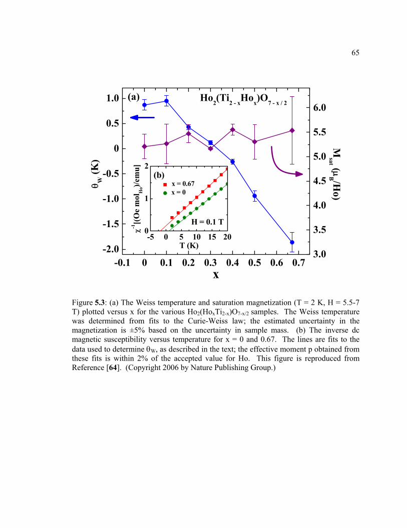
65

-5 0 5 10 15 200

1

2

3.0

3.5

4.0

4.5

5.0

5.5

6.0

-0.1 0 0.1 0.2 0.3 0.4 0.5 0.6 0.7-2.0

-1.5

-1.0

-0.5

0

0.5

1.0

Msat (μ

B /Ho)

θ W (K

)

x

Ho2(Ti2 - xHox)O7 - x / 2(a)

H = 0.1 T

x = 0.67 x = 0

χ-1[(

Oe

mol

Ho)/e

mu]

T (K)

(b)

Figure 5.3: (a) The Weiss temperature and saturation magnetization (T = 2 K, H = 5.5-7 T) plotted versus x for the various Ho2(HoxTi2-x)O7-x/2 samples. The Weiss temperature was determined from fits to the Curie-Weiss law; the estimated uncertainty in the magnetization is ±5% based on the uncertainty in sample mass. (b) The inverse dcmagnetic susceptibility versus temperature for x = 0 and 0.67. The lines are fits to thedata used to determine θW, as described in the text; the effective moment p obtained from these fits is within 2% of the accepted value for Ho. This figure is reproduced fromReference [64]. (Copyright 2006 by Nature Publishing Group.)

66

0 0.1 0.2 0.3 0.4 0.5 0.6 0.7

-5

-4

-3

-2

-1

0

0 10 200

1

2

0 1 2 3 4 50

1

2

3

4

5

( b )

( c )

Dyx(Ti2-xDyx)O7-x/2

θ W [

K ]

x

( a )

H = 0.1 T

x = 0.67 x = 0

1 / χ

[ em

u / (

Oe

mol

Dy )

]

T [ K ]

M [

μ B /

Dy

]

H [ T ]

x = 0 0.1 0.2 0.3 0.4 0.5 0.67T = 2 K

Figure 5.4: Magnetization data for Dy2(DyxTi2-x)O7-x/2, 0 ≤ x ≤ 0.67. (a) The Weiss Temperature θW as a function of stuffing x was obtained from fits to data taken in a field of H = 0.1 T. Examples of the fits are shown in (b). (c) M(H) at T = 2 K for each valueof x.

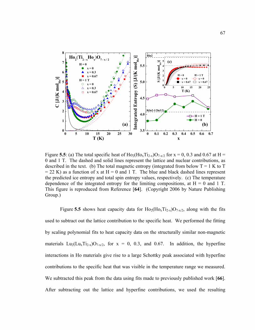
67

Figure 5.5 shows heat capacity data for Ho2(HoxTi2-x)O7-x/2, along with the fits

used to subtract out the lattice contribution to the specific heat. We performed the fitting

by scaling polynomial fits to heat capacity data on the structurally similar non-magnetic

materials Lu2(LuxTi2-x)O7-x/2, for x = 0, 0.3, and 0.67. In addition, the hyperfine

interactions in Ho materials give rise to a large Schottky peak associated with hyperfine

contributions to the specific heat that was visible in the temperature range we measured.

We subtracted this peak from the data using fits made to previously published work [66].

After subtracting out the lattice and hyperfine contributions, we used the resulting

0 5 10 15 20 25 300

1

2

3

4

5

6

7

8

0 5 10 15 20 250

1

2

3

4

5

0 0.1 0.2 0.3 0.4 0.5 0.6 0.73.5

4.0

4.5

5.0

5.5H = 0 x = 0 x = 0.3 x = 0.67

H = 1 T x = 0 x = 0.3 x = 0.67

T (K)

Ho2(Ti2 - xHox)O7 - x / 2C

[J/(K

mol

Ho)]

(a)

H = 0 H = 1 T x = 0 x = 0 x = 0.67 x = 0.67

T (K)

S [J

/(K m

olH

o)] (c)

R(ln2-1/2ln3/2)

(b)

H = 1 T H = 0

x

Inte

grat

ed E

ntro

py (S

) [J/

(K m

olH

o)] Rln2

Figure 5.5: (a) The total specific heat of Ho2(HoxTi2-x)O7-x/2 for x = 0, 0.3 and 0.67 at H = 0 and 1 T. The dashed and solid lines represent the lattice and nuclear contributions, asdescribed in the text. (b) The total magnetic entropy (integrated from below T = 1 K to T= 22 K) as a function of x at H = 0 and 1 T. The blue and black dashed lines representthe predicted ice entropy and total spin entropy values, respectively. (c) The temperaturedependence of the integrated entropy for the limiting compositions, at H = 0 and 1 T. This figure is reproduced from Reference [64]. (Copyright 2006 by Nature Publishing Group.)

68

magnetic specific heat to determine the total magnetic entropy from Equation 5.2 by

assuming that S = 0 at T = 0, which is valid since there was no significant contribution to

the entropy below the temperature range of our measurements. Panel (c) in Figure 5.5

shows S(T) for the x = 0 and x = 0.67 samples at fields of H = 0 and 1 T, illustrating the

climb in S(T) with temperature for large values of c/T, and that S(T) stabilizes at some

total value once c/T ~ 0. For x = 0 and H = 0 the entropy rises to the spin ice value, in

agreement with previously published work [66][68]. The total value of the magnetic

entropy at T = 22 K for each value of x is shown in panel (b) of Figure 5.5, where every

point represents the average of at least two separate measurements on different samples

for each value of x. Surprisingly, the entropy at H = 0 remains at the spin ice value for all

x, within the ± 10% uncertainty caused by the uncertainty in the sample mass. At H = 1

T, the total entropy grows towards S = Rln2 for x = 0, and again stays at a constant value

for all x.

To contrast with the Ho2(HoxTi2-x)O7-x/2 data, we show specific heat data for

Dy2(DyxTi2-x)O7-x/2 in Figure 5.6. The left panel shows the specific heat after subtracting

out the contributions due to the Ag used in preparing the sample for measurement. The

lattice contributions were again subtracted out by scaling data on Lu2(LuxTi2-x)O7-x/2, x =

0, 0.3, and 0.67, using the same procedure as in the Ho2(HoxTi2-x)O7-x/2 data. Unlike the

Ho samples, the Schottky peak due to hyperfine interactions does not appear in these

measurements, resulting in a simpler determination of the magnetic specific heat by

merely subtracting out the lattice contributions. As shown in the inset to the left panel,

we again obtain the total magnetic entropy by integrating the magnetic specific heat and

assuming S = 0 at T = 0. The right panel in Figure 5.6 shows the total magnetic entropy

69

as a function of stuffing for Dy2(DyxTi2-x)O7-x/2 at H = 0 and 1 T, along with the H = 0

total magnetic entropy for Ho2(HoxTi2-x)O7-x/2. Again, the points in this figure are the

average of multiple measurements for each value of x, and the error primarily depends on

the uncertainty in the sample mass. The two error bars shown represent the typical

uncertainty for each point. Clearly, for x < 0.3, the total entropy for the Dy materials

monotonically increases away from the spin ice value towards S = Rln2, and then

remains constant, within error, up to x = 0.67. Application of a magnetic field restores

some of the residual entropy in the x = 0 sample, in agreement with previous results [63].

For higher x, the total entropy in a H = 1 T field stays at the x = 0 value.

To further investigate these systems, AC susceptibility experiments were

performed on x = 0.67 samples of both materials. The data were independent of the AC

0 5 10 15 20 25 300

2

4

6

8

Dy2( Ti2 - xDyx ) O7

x = 0 0.3 0.67

c P [ J

/ ( K

mol

Dy )

]

T [ K ]

H = 0

0 0.1 0.2 0.3 0.4 0.5 0.6 0.7

4.0

4.5

5.0

5.5

6.0

Ho2( Ti2 - xHox ) O7

H = 0 1 T

R ln 2Dy2( Ti2 - xDyx ) O7

S tota

l [ J

/ ( m

olD

y K )

]

x

Spin Ice

0 5 10 150

2

4

6

S [ J

/ ( m

olD

y K )

]

T [ K ]

Figure 5.6: (left) The specific heat of Dy2(DyxTi2-x)O7-x/2, x = 0, 0.3, 0.67, at H = 0. The inset shows the H = 0 magnetic entropy obtained by integrating the specific heat from atleast T = 0.5 K, after subtracting out scaled specific heat data on nonmagneticLu2(LuxTi2-x)O7-x/2, x = 0, 0.3, 0.67, (shown as dashed lines in the main graph). (right)The total magnetic entropy of Dy2(DyxTi2-x)O7-x/2, 0 ≤ x ≤ 0.67, at H = 0, 1 T, and 1.5 T. The solid line shows the corresponding total entropy for Ho2(HoxTi2-x)O7-x/2 at H = 0.

70

excitation field used, which was Hac < 1 Oe for all of the measurements. For the Ho case,

the large hyperfine effects seen in the specific heat will not appear in the AC

susceptibility measurements, yielding a clearer picture of the electronic magnetism in the

sample. Additionally, since low temperature AC susceptibility measurements have been

previously performed on Ho2Ti2O7 and Dy2Ti2O7, data on the x = 0.67 sample can be

compared to a good base set of data [69][71].

Figure 5.7 shows the real part of the H = 0 AC susceptibility versus temperature

for Ho2.67Ti1.33O6.67 (x = 0.67) at various frequencies. The data are calibrated using χ′(H)

data from the ACMS, with an estimated error of ± 1% in calibration. While

0 1 2 3 40

0.5

1.0

1.5

2.0

2.5

3.0

0 0.5 1.0 1.5 2.0

0

0.05

0.10

0.15

0.20

f = 10 Hz 50 Hz 100 Hz 500 Hz 1 kHz

Ho2.67Ti1.33O6.67 H = 0

χ′ [

emu

/ ( O

e m

olH

o ) ]

Temperature [ K ]

χ′′ [

em

u / (

Oe

mol

Ho )

]

Temperature [ K ]

Figure 5.7: The real and imaginary parts of the H = 0 AC susceptibility versustemperature of Ho2.67Ti1.33O6.67 for various measurement frequencies. Data above T > 2K was taken with the ACMS, while data taken below T = 2 K was taken in the dilutionrefrigerator. The inset shows the imaginary part of the susceptibility taken from dilutionrefrigerator measurements.

71

paramagnetic behavior occurs at high temperature, below T = 2 K a frequency dependent

peak in the susceptibility forms, with maxima occurring at T ≈ 1.4 K for f = 10 Hz and T

≈ 1.7 K for f = 1 kHz. This peak is quite similar to the peak seen in χ′(T) for Ho2Ti2O7,

although its magnitude is much smaller. The presence of the frequency dependent

maximum indicates a possible spin freezing at the measurement frequencies and at

temperatures corresponding to the magnitude of θW shown in Figure 5.3. After the

maximum, the susceptibility tends towards zero as T ~ 0 for each frequency measured.

The inset to Figure 5.7 shows a corresponding frequency dependent peak in χ''(T) at the

same temperatures, as expected from the Kramers – Kronig relations.

Next, Figure 5.8 shows χ′(T) and χ''(T) at H = 0 for Dy2.67Ti1.33O6.67 for various

measurement frequencies. The data here are again calibrated using χ′(H) data from the

ACMS, with an estimated error in the calibration of ± 1%. As in the data for

Ho2.67Ti1.33O6.67, χ′(T) shows a frequency dependent peak ending the high temperature

paramagnetic behavior. The peak develops at T < 2.5 K and reaches a maximum at T ≈

1.7 K for f = 10 Hz and at T ≈ 1.9 K for f = 100 Hz., indicating that spins are freezing at

these temperatures. The inset shows that for T > 0.75 K, χ''(T) has a corresponding

frequency dependent maximum, again indicating that at least some of the spins are

freezing. However, in contrast with the Ho2.67Ti1.33O6.67 data, χ′(T) retains a strong

frequency dependence and does not appear to go to zero as T ~ 0. Though unusual, this

behavior occurs in some spin glasses and in some geometrically frustrated magnets which

display cooperative paramagnetic behavior at low temperatures [20][47].

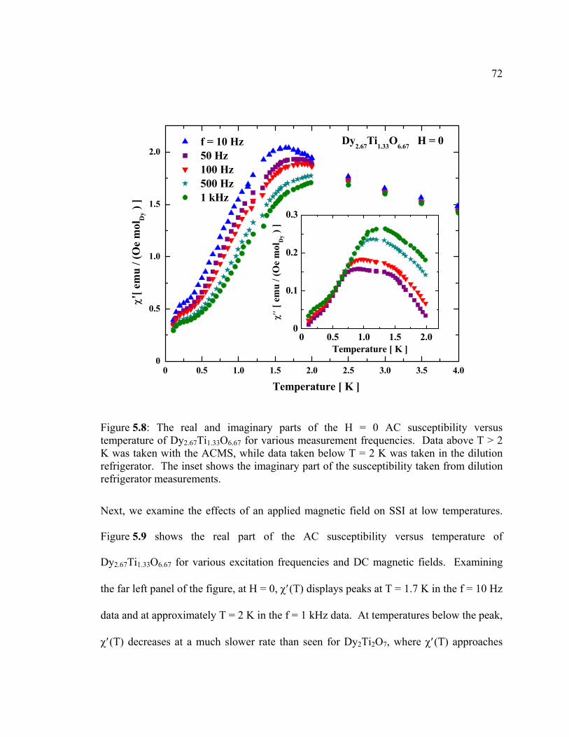
72

Next, we examine the effects of an applied magnetic field on SSI at low temperatures.

Figure 5.9 shows the real part of the AC susceptibility versus temperature of

Dy2.67Ti1.33O6.67 for various excitation frequencies and DC magnetic fields. Examining

the far left panel of the figure, at H = 0, χ′(T) displays peaks at T = 1.7 K in the f = 10 Hz

data and at approximately T = 2 K in the f = 1 kHz data. At temperatures below the peak,

χ′(T) decreases at a much slower rate than seen for Dy2Ti2O7, where χ′(T) approaches

0 0.5 1.0 1.5 2.0 2.5 3.0 3.5 4.00

0.5

1.0

1.5

2.0

0 0.5 1.0 1.5 2.00

0.1

0.2

0.3

f = 10 Hz 50 Hz 100 Hz 500 Hz 1 kHz

Dy2.67Ti1.33O6.67 H = 0

χ'[ e

mu

/ (O

e m

olD

y ) ]

Temperature [ K ]

χ′′ [

em

u / (

Oe

mol

Dy )

]

Temperature [ K ]

Figure 5.8: The real and imaginary parts of the H = 0 AC susceptibility versustemperature of Dy2.67Ti1.33O6.67 for various measurement frequencies. Data above T > 2 K was taken with the ACMS, while data taken below T = 2 K was taken in the dilutionrefrigerator. The inset shows the imaginary part of the susceptibility taken from dilutionrefrigerator measurements.

73

zero below T = 0.5 K [69][71]. As the magnetic field is increased, the magnitude of the

peak diminishes, while its frequency dependence appears to be substantially affected only

in the H = 2 T data. The frequency dependence of the temperature of the peak is

indicative of a spin glass, however the fact that the peak does not shift in temperature and

is not substantially broadened by even a field of H = 1 T appears to rule out a typical spin

glass state at low temperatures.

Figure 5.10 shows f = 50 Hz χ′(H) data for Ho2.67Ti1.33O6.67 at T = 0.3 K and 1.8

K, while increasing the magnetic field at 0.01 T/min and 0.1 T/min, respectively. The

data show typical behavior for magnetic saturation at T = 1.8 K and a diminished

susceptibility at T = 0.3 K. The small value of χ′(H) at low fields for T = 0.3 K reflects

the spin freezing occurring below T = 1.7 K. Unfortunately, we were not able to take

data at more temperatures. However, we will next show χ(H) data on Dy2.67Ti1.33O6.67 at

various low temperatures.

0 1 2 30

0.5

1.0

1.5

2.0

0 1 2 3 0 1 2 3 0 1 2 3 4

f = 10 Hz 100 Hz 1 kHz

χ′ [

emu

/ ( O

e m

olD

y ) ] H = 0 0.5 T

T [ K ]

1 T

2 T

Figure 5.9: The field dependence of the real part of the AC susceptibility versustemperature of Dy2.67Ti1.33O6.67 for various measurement frequencies. Each panel showsdata taken at a different applied magnetic field (H = 0 – 2 T, from left to right).

74

χ′(H) and χ''(H) for Dy2.67Ti1.33O6.67 at T ≤ 1.8 K and f = 50 Hz are plotted in

Figure 5.11, where we made measurements while sweeping the field at a rate of

0.001T/min to ensure equilibrium conditions. The data show two peaks forming in χ′(H)

at lower temperatures, with corresponding peaks occurring in χ′′(H). For H < 3 T, χ′(H)

decreases and flattens out with decreasing temperature, until the temperature becomes

low enough for another peak to form in χ′(H). The imaginary part of the susceptibility

rises and falls at the two peaks in χ′(H) and plateaus in between.

0 1 2 30

0.5

1.0

1.5

2.0

2.5

T = 1.8 K0.3 K

Ho2.67Ti1.33O6.67 f = 50 Hz

χ′ [

emu

/ ( O

e m

olH

o ) ]

H [ T ]

0 2 4 6 80

1

2

3

4

5

Μ [

μ B /

Ho

]

H [ T ]

Figure 5.10: The f = 50 Hz AC susceptibility versus applied DC field of Ho2.67Ti1.33O6.67, at various temperatures. Data were taken at T = 0.3 K and T = 1.8 K while sweeping thefield at rates of 0.01 T/min and 0.1 T/min, respectively. The inset shows M(H) for T ≤ 1.8 K, determined by integrating χ′(H).

75

The insets to Figures 5.10 and 5.11, show the magnetization versus field of each

sample obtained by integrating χ′(H). At T = 1.8 K the data saturates at M ~ 5 μB, in

agreement with the data in Figures 5.3 and 5.4. At lower temperatures, M(H) saturates at

a slower rate, which is consistent with the AFM spin-spin interactions becoming more

important. Furthermore, M(H) of Dy2.67Ti1.33O6.67 at T = 0.2 K and 0.085 K, does not

even reach M = 2μB/Dy by H = 1.5 T, and the AC susceptibility is going towards zero at

0

0.5

1.0

1.5

2.0

0 0.5 1.0 1.5 2.0 2.5 3.0

0

0.05

0.10

0.15

T = 1.8 K1.5 K 0.9 K 0.6 K 0.2 K 0.085 K

f = 50 Hz

χ′ [

emu

/ ( O

e m

olD

y ) ]

Dy2.67Ti1.33O6.67

χ′′ [

em

u / (

Oe

mol

Dy )

]

H [ T ]

0 1 2 3 40.1

1

105 μB / Dy

M [

μ B /

Dy

]

H [ T ]

∫ χ′ dH50 Hz

Figure 5.11: The f = 50 Hz AC susceptibility versus applied DC field of Dy2.67Ti1.33O6.67, at various temperatures. Data was taken while sweeping the field at a rate of 10 Oe/min.The inset shows M(H) for T ≤ 1.8 K, determined by integrating χ′(H). Note the log scale on the inset’s vertical axis.

76

higher fields. This means that more than half of moment in Dy2.67Ti1.33O6.67 may be

frozen out at these temperatures due to spin-spin interactions. This is in stark contrast to

data for Dy2Ti2O7 and other spin ice materials, which show M ~ 4 μB by H = 1.5 T at T =

0.25 K [69][71].

5.5 Discussion

We now discuss the data on the Ho and Dy SSI materials and start by looking at

the similar behavior in the DC magnetization results in Figures 5.3 and 5.4. The

increasingly AFM behavior of θW with increasing x seen for both the Ho and Dy samples

suggest that the alteration of the lattice with stuffing does not drastically change the

interactions between the magnetic cations on the A-sites because of the higher level of Ti

disorder in the Ho materials, as seen in Figure 5.2. Rather, we conclude that the magnetic

interactions between the A and B-sites are antiferromagnetic, and that increasing the

number of such pairs creates a more AFM θW at larger x. Additionally, as previously

discussed, the M(H) data suggest that the single ion ground state remains Ising like in

both the Ho and Dy SSI, since the saturated magnetization remains constant for all values

of stuffing.

Moving on to the heat capacity data in Figures 5.5 and 5.6, the T ≈ 2 K peaks in

the specific heat are broader at higher values of stuffing for both Ho2(HoxTi2-x)O7-x/2 and

Dy2(DyxTi2-x)O7-x/2. Broad peaks in c(T) can indicate the presence of short range

correlations between spins, and since the peak in our data appears wider for larger x, it is

possible that the additional AFM interactions from stuffing lead to more correlations

77

developing between spins. This is reasonable since AFM coupled Ising spins with [111]

anisotropy on the pyrochlore lattice can form the all in, all out (Q = 0) long range ordered

state [53][62]. However, the fact that the entropy approaches S = Rln2 for

Dy2.67Ti1.33O6.67 but not for Ho2.67Ti1.33O6.67 can not be explained using the heat capacity

data alone.

To clarify the reasons behind the difference between the total entropy for

Ho2.67Ti1.33O6.67 and Dy2.67Ti1.33O6.67, we turn to the AC susceptibility data in Figures 5.7

and 5.8, where we see that the low temperature susceptibilities of the two materials are

somewhat different. For Ho2.67Ti1.33O6.67, the maximum in χ′(T) is followed by a steady

drop to χ′(T) ~ 0 at T ~ 0 indicating that most (if not all) of the spins in the material

freeze at low temperature, while the frequency dependence of the temperature of the

maximum suggests an absence of long range magnetic order. This situation is quite

similar to χ′(T) for Ho2Ti2O7, where the large energy barriers in the material cause the

Ho to freeze into the disordered spin ice state [30][51][70][72]. However, in our case

χ′(T) ~ 0 only as T ~ 0, not at a finite temperature as in pure spin ice [69]. This may

indicate that the additional magnetic interactions and the disorder in the lattice alter the

spin relaxation pathways in Ho2.67Ti1.33O6.67 permitting the spins to fluctuate down to

much lower temperatures, yet still show a complete freezing as T ~ 0.. Since the total

entropy remains around the ice value, we therefore conclude that Ho2.67Ti1.33O6.67 freezes

below T ≈ 2 K into a disordered state showing both glassy and ice like properties

analogous to pure spin ice.

78

Turning now to Dy2.67Ti1.33O6.67, Figure 5.8 shows that the maximum in χ′(T) for

Dy2.67Ti1.33O6.67 also has some frequency dependence, however, contrary to the data for

Ho2.67Ti1.33O6.67 the susceptibility seemingly does not approach zero as T ~ 0. Also, the

frequency dependence of χ′(T) strongly persists down to T ~ 0 for Dy2.67Ti1.33O6.67. As

previously stated and discussed more below, such behavior occurs in some spin glasses

and cooperative paramagnets (i.e. spin liquids) [20][31][41][47]. Next, we see in

Figure 5.11 that two maxima in χ′(H) for Dy2.67Ti1.33O6.67 at low temperatures with a

corresponding plateau in χ''(H). As seen in the inset to the figure, the peak at higher field,

followed by the decrease to χ′(H) = 0 at high fields is due to the field completely

saturating single spins. However, the peak in χ′(H) at lower temperatures obviously does

not represent single spin saturation, since a finite susceptibility remains at fields above

the peak. One possible explanation is that the low field maximum in χ′(H) seen at low

temperatures represents the energy due to the field beginning to dominate the interactions

between spins. Such a situation has been seen in AC susceptibility data on GGG, in

which a broad peak develops in χ′(H) at low temperatures, corresponding to the field

quenching the short range AFM order between spins [76]. Taking this interpretation of

the low field maximum in χ′(H) together with the fact that χ′(T) retains a finite value T ~

0, leads us to conclude that Dy2.67Ti1.33O6.67 may have a cooperative paramagnet type

state at low temperatures among at least some of its spins.

Our data also compare well to results from studies on different cooperative

paramagnets and spin liquids. For example, specific heat and susceptibility data on the

cooperative paramagnets Tb2Ti2O2 and Tb2Nb2O7, which both have a pyrochlore lattice,

79

show that the expected total entropy per Tb is recovered at temperatures corresponding to

the effective magnetic interactions, while their susceptibilities remain finite as T ~ 0

[20][31][41][47]. This compares well with our data in Figure 5.6, which show the total

entropy per Dy in Dy2.67Ti1.33O6.67 rapidly rising at T ≈ 4 K, approaching the expected

value for an Ising system of S = Rln2, and our data in Figure 5.8, which show a finite

susceptibility for Dy2.67Ti1.33O6.67 as T ~ 0. Additionally, frequency dependent peaks in

χ′(T) similar to those seen in Figures 5.8 and 5.9 indicative of a spin glass type freezing

are seen in data on Tb2Ti2O7, and the spin liquids Gd3Ga5O12 (GGG) [77][78] and

SrCr9pGa12-9pO19 (SCGO) [79][80]. Furthermore, susceptibility, neutron scattering, and

Muon spin resonance data on Tb2Ti2O7 and SCGO show the persistence of spin

fluctuations even after partial spin freezing occurs [29][37][38][81][82][83].

5.6 Conclusion

Though we have not proven that Dy2.67Ti1.33O6.67 is a cooperative paramagnet,

creating a liquid like state by adding competing interactions to an ice state is quite

intriguing, and any sensitivity of such a transformation to the Ti disorder in

Ho2.67Ti1.33O6.67 is curious. Subsequent studies involving AC susceptibility and neutron

scattering measurements on both powders and single crystals of Ho2(HoxTi2-x)O7-x/2 and

Dy2(DyxTi2-x)O7-x/2 for different values of x need to be performed before any solid

conclusions can be made. Nevertheless, the energy scales involved in these materials

allow probing of their properties by many different techniques, and further experiments

80

on these materials will undoubtedly shed light into the development of correlations and

order within materials.

Bibliography

1. F. Reif, Fundamentals of Statistical and thermal Physics, McGraw-Hill, Boston (1965).

2. R.K. Pathria, Statistical Mechanics, Butterworth-Heinemann, Oxford (2001).

3. R.M. White, Quantum Theory of Magnetism, Springer, New York (1983).

4. N.W. Ashcroft and N.D. Mermin, Solid State Physics, Harcourt Brace, USA (1976).

5. C. Kittel, Introduction to Solid State Physics, John Wiley & Sons, Inc., New York (1996).

6. A.H. Morrish, The Physical Principles of Magnetism, John Wiley & Sons, Inc., New York (1965).

7. F. Bloch, Phys. Rev. 70, 460 (1946).

8. A. Abragam and B. Bleaney, Electron Paramagnetic Resonance of Transition Ions, Dover Publications, New York (1986).

9. A. Schenck, Muon Spin Rotation Spectroscopy: Principles and Applications in Solid State Physics, A. Hilger, Boston (1985).

10. G.L. Squires, Introduction to the Theory of Thermal Neutron Scattering, Cambridge University Press, Cambridge (1978).

11. H.B.G. Casimir and F.K. du Pré, Physica 5, 507 (1938).

12. J.D. Jackson, Classical Electrodynamics, John Wiley & Sons, Inc., New York (1999).

13. G. Arfken, Mathematical Methods for Physicists, Academic Press, San Diego (1995).

14. K.W.H. Stevens, Rep. Prog. Phys. 30, 189 – 226 (1967).

15. P. Schiffer and A. P. Ramirez, Comments on Condensed Matter Physics 18, 21-50 (1996).

16. A.P. Ramirez, in Handbook of Magnetic Materials, Ed. K. J. H. Buschow, New Holland, New York, 423-520, (2001).

82

17. H.T. Diep, Magnetic Systems with Competing Interactions, World Scientific, Singapore (1994)

18. H.T. Diep, Frustrated Spin Systems, World Scientific, Singapore (2004).

19. R. Moessner, Can. J. Phys. 79, 1283 – 1294 (2001).

20. J.A. Mydosh, Spin Glasses, Taylor and Francis, London (1993).

21. S. Nagata, P.H. Keesom, and H.R. Harrison, Phys. Rev. B 19, 1633 (1979).

22. D. Hüser et al., Phys. Rev. B 27, 3100 (1983).

23. J.R.L. de Almeida and D.J. Thouless, J. Phys. A11, 983 (1978).

24. M. Gabay and G. Toulouse, Phys. Rev. Lett. 47, 201 (1981).

25. I.S. Hagemann et al., Phys. Rev. Lett. 86, 894 (2001).

26. D. Bono et al., Phys. Rev. Lett. 92, 217202 (2004).

27. A. Olariu et al., Phys. Rev. Lett. 97, 167203 (2006).

28. B.G. Ueland et al., Phys. Rev. Lett. 96, 027216 (2006).

29. J.S. Gardner et al., Phys. Rev. B 68, 180401(R) (2003).

30. J. Snyder et al., Phys. Rev. Lett. 91, 107201 (2003).

31. M.J.P. Gingras et al., Phys. Rev. B 62, 6496 (2000).

32. Y.K. Tsui et al., Phys. Rev. Lett. 82, 3532 (1999).

33. Quantum Design, Inc. 6325 Lusk Boulevard, San Diego CA 92121.

34. R.C. Richardson and E.N. Smith, Experimental Techniques in Condensed Matter Physics at Low Temperatures, Addison-Wesley Publishing Company, Inc., Reading (1988).

35. J. Villain, Z. Phys. B 33, 31 (1979).

36. A. P. Ramirez et al., Phys. Rev. Lett. 84, 2957 (2000) and references therein.

37. J.S. Gardner et al., Phys. Rev. Lett. 82, 1012 (1999).

38. Y. Yasui et al., J. Phys. Soc. Jpn. 71, 599 (2002).

39. J.S. Gardner et al., Phys. Rev. B 64, 224416 (2001).

83

40. M. Kanada et al., J. Phys. Soc. Jpn. 68, 3802 (1999).

41. Y.M. Jana et al., Phys. Rev. B 68, 174413 (2003).

42. I.V. Aleksandrov et al., Sov. Phys. JETP 62, 1287 (1985).

43. S. Rosenkranz et al., J. Appl. Phys. 87, 5914 (2000).

44. I. Mirebeau et al., Nature 420, 54 (2002).

45. K.C. Rule et al., Phys. Rev. Lett. 96, 177201 (2006).

46. G. Luo, S.T. Hess, and L.R. Corruccini, Phys. Lett. A 291, 306 (2001).

47. N. Hamaguchi et al., Phys. Rev. B 69, 132413 (2004).

48. B.G. Ueland, unpublished.

49. M. J. Harris et al., Phys. Rev. Lett. 79, 2554 (1997).

50. J.H. Van Vleck, The Theory of Electric and Magnetic Susceptibilities, Oxford University Press, London (1959).

51. J. Snyder et al., Phys. Rev. B 70, 184431 (2004).

52. R. Siddharthan et al., Phys. Rev. Lett. 83, 1854 (1999).

53. B.C. den Hertog and M. J. P. Gingras, Phys. Rev. Lett. 84, 3430 (2000).

54. S.V. Isakov, R. Moessner, and S.L. Sondhi, Phys. Rev. Lett. 95, 217201 (2005).

55. A. Keren et al., Phys. Rev. Lett. 92, 107204 (2004).

56 R. Mahendiran et al., Phys. Rev. B 68, 104402 (2003) and references therein.

57. J.D. Bernal and R.H. Fowler, J. Chem. Phys. 1, 515 (1933).

58. W.F. Giaque and J.W. Stout, J. Am. Chem. Soc. 58, 1144 – 1150 (1936).

59. L. Pauling, The Nature of the Chemical Bond, Cornell University Press, Ithaca (1945).

60. G.H. Wannier, Phys. Rev. 79, 357 (1950).

61. P.W. Anderson, Phys. Rev. 102, 1008 (1956).

62. S.T. Bramwell and M.J. Harris, J. Phys.: Condens. Matter 10, L215 (1998).

84

63. A.P. Ramirez et al., Nature 399, 333 (1999).

64. G.C. Lau et al., Nat. Phys. 2, 249 (2006).

65. B.G. Ueland et al., manuscript in preparation.

66. S.T. Bramwell et al., Phys. Rev. Lett. 87, 047205 (2001).

67. R.G. Melko et al., cond-mat/0308282.

68. A.L. Cornelius and J.S. Gardner, Phys. Rev. B 64, 060406R (2001).

69. K. Matsuhira et al., J. Phys.: Condens. Matter 12, L649 (2000).

70. K. Matsuhira, Y. Hinatsu, and T. Sakakibara, J. Phys.: Condens. Matter 13, L737 (2001).

71. J. Snyder et al., Phys. Rev. B 69, 064414 (2004).

72. J. Snyder et al., Nature 413, 48 (2001).

73. G Ehlers et al., J. Phys.: Condens. Matter 15, L9 (2003).

74. G.C. Lau et al., J. Solid State Chem. 179, 3126 (2006).

75. H. Fukazawa et al., Phys. Rev. B 65,054410 (2002).

76. P. Schiffer et. al., Phys. Rev. Lett 73, 2500 (1994).

77. P. Schiffer et. al., Phys. Rev. Lett 74, 2379 (1995).

78. Y.K. Tsui, J. Snyder, and P. Schiffer, Phys. Rev. B 64, 012412 (2001).

79. A.P. Ramirez et. al., Phys. Rev. Lett. 64, 2070 (1990).

80. A.P. Ramirez et. al., Phys. Rev. B 45, 2505 (1992).

81. C. Broholm et. al., Phys. Rev. Lett. 65, 3173 (1990).

82. Y.J. Uemura et. al., Phys. Rev. Lett. 73, 3306 (1994).

83. P. Schiffer et. al., Phys. Rev. Lett 77, 1085(1996).

Appendix A

AC Susceptibility Measurements on a Dilution Refrigerator

A.1 Schematic of the Electrical Circuits Used for AC Susceptibility Measurements

Figure A.1: The electrical circuits used to measure the AC susceptibility as described inSection 3.12.3. For most of the measurements, the secondaries were connected to apreamplifier located before the secondary lock-in amplifier. All experimental connections between the dilution refrigerator and external instruments were made usingcoaxial cables with BNC connectors. The resistances used in the primary circuit were R1

= 48.2 Ω and R2 = 1.085 kΩ, and the ground for the primary circuit was taken at theshield of the BNC connector supplying the AC voltage. The reference phase for thesecondary lock-in was taken between one of the R2 resistors and the primary circuit’s ground.

P

SS

VViVi

ωχχ

′+′′−∝′′+′

SecondaryLock-in Amplifier

PrimaryLock-in Amplifier

Reference Phase

Appliedac Voltage

VR

R1

VSB

A A

B

R2

R2

ac

ns = 1018 turns / 1 cmnP = 848 turns / 3.4 cm

= 249.4 turns/cm@ 1V, Hac = 0.1 Oe

np

ns

ns

sample

P

SS

VViVi

ωχχ

′+′′−∝′′+′

SecondaryLock-in Amplifier

PrimaryLock-in Amplifier

Reference Phase

Appliedac Voltage

VR

R1

VSB

A A

B

R2

R2

ac

ns = 1018 turns / 1 cmnP = 848 turns / 3.4 cm

= 249.4 turns/cm@ 1V, Hac = 0.1 Oe

np

ns

ns

sample

P

SS

VViVi

ωχχ

′+′′−∝′′+′

SecondaryLock-in Amplifier

PrimaryLock-in Amplifier

Reference Phase

Appliedac Voltage

VR

R1

VSB

A A

B

R2

R2

ac

ns = 1018 turns / 1 cmnP = 848 turns / 3.4 cm

= 249.4 turns/cm@ 1V, Hac = 0.1 Oe

np

ns

ns

sampleSecondary

Lock-in Amplifier

PrimaryLock-in Amplifier

Reference Phase

Appliedac Voltage

VR

R1

VSB

A A

B

R2

R2

ac

SecondaryLock-in Amplifier

PrimaryLock-in Amplifier

Reference Phase

Appliedac Voltage

VR

R1

VSB

A A

B

R2

R2

ac

ns = 1018 turns / 1 cmnP = 848 turns / 3.4 cm

= 249.4 turns/cm@ 1V, Hac = 0.1 Oe

np

ns

ns

sample

86

A.2 Procedure for Converting the Measured Voltage to Susceptibility

Converting the voltage signal received by the secondary lock-in amplifier into a

measure of magnetic susceptibility relies on Faraday’s Law (Equation 3.1). Labeling the

secondary coil containing the sample as coil 1 and the empty secondary coil as coil 2, we

can write the induced EMF in the circuit in CGS units as Equation A.1:

where the magnetic flux φ going through each coil is equal to the magnitude of the

magnetic field along the axis of the coil times the coil’s cross sectional area. Since both

secondaries have equal dimensions, we can label the number of turns of wire in each

secondary as Ns and the cross sectional area of each as As. Remembering that we can

write the magnetic field B inside of each coil as Equation A.2:

then the total EMF induced in the secondary circuit by an external magnetic field H is

Equation A.3:

where the negative sign in front of the cross sectional area for coil 2 results from the coils

being wound in opposite directions. We can easily see from Equation A.3 that balancing

the secondary coils cancels out any EMF induced by a field simultaneously present in

⎟⎠

⎞⎜⎝

⎛+−=

dtd

dtd

cE 211 φφ

, (A.1)

MHB π4+= , (A.2)

⎟⎠⎞

⎜⎝⎛ −+

+−= ssss NA

dtdHAN

dtMHd

cE )()4(1 π , (A.3)

87

both coils. Hence, when we apply an alternating field to the coils, only the response of

the magnetization of the sample in coil 1 produces an EMF, yielding Equation A.4:

We then rewrite Equation A.4 as Equation A.5 using the definition for the susceptibility

of a magnet in a small field:

where f is called the filling factor of the coil and depends on the volume of the coil

occupied by the sample.

Next, we use the infinite solenoid approximation and Ampere’s Law to derive the

field H created by the primary coil. We start by defining n as the number of turns per

unit length of the coil and j as the current in each loop of wire. This leads to

Equation A.6:

If we assume that j changes periodically in time at an angular frequency ω, then H will

also be time dependent and we can again rewrite Equation A.5 , yielding Equation A.7:

followed by Equation A.8:

dtdMAN

cE ss

π4−= . (A.4)

( )dt

HfdANc

E ssχπ4

−= , (A.5)

njc

H π4= . (A.6)

( )dt

tijdnfANc

E ssωχπ exp(4 2

⎟⎠⎞

⎜⎝⎛−= (A.7)

( )tijnfANc

iE ss ωωχπ exp4 2

⎟⎠⎞

⎜⎝⎛−= . (A.8)

88

Now, we write E as a time dependent quantity with the same frequency as H giving

Equation A.9:

which leads to Equation A.10:

Finally, writing V and χ as complex variables and equating real and imaginary parts

gives Equations A.11 and A.12:

)exp( tiVE ω= , (A.9)

ωχπ jnfANc

iV ss

24⎟⎠⎞

⎜⎝⎛−= . (A.10)

fnjANVc

ss ωπχ

′′⎟⎠⎞

⎜⎝⎛−=′

2

4 (A.11)

fnjANVc

ss ωπχ

′⎟⎠⎞

⎜⎝⎛=′′

2

4. (A.12)

Appendix B

Demagnetization Effects

The purpose of this appendix is to introduce the concept of demagnetization

effects on magnetic samples and show their relevance to the experiments performed for

this thesis.

When an external magnetic field H polarizes a uniform magnetic material, the

magnetization of the sample creates an internal field [H' – H] that, in general, changes the

effective field acting on the material. Following the discussion given in Morrish [6], for

a uniform ferromagnetic material with an ellipsoidal shape lying with its long axis along

the external field, we can picture north and south magnetic poles appearing on opposing

sides of the sample as in Figure B.1. Mathematically, for a sample with magnetization

per unit volume M, Equation B.1 gives the correct internal field as:

where D is a tensor describing a shape dependent demagnetization factor, and tables

listing the values of D for different shapes are available [6].

For our purposes, we will consider two shapes: a sphere and a long thin ellipsoid

of revolution. The case of a sphere may apply to our powder samples, because we can

consider the particulates to be micron sized spherical crystals. However, in practice it

may be more practical to look at the bulk shape of the powder while it is measured.

Since previous studies disagree on the proper treatment for the demagnetization effects in

a powder sample, we will simply consider here a large single crystalline sphere. Also, we

DMHH −=′ , (B.1)

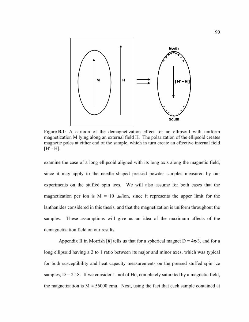
90

examine the case of a long ellipsoid aligned with its long axis along the magnetic field,

since it may apply to the needle shaped pressed powder samples measured by our

experiments on the stuffed spin ices. We will also assume for both cases that the

magnetization per ion is M = 10 μB/ion, since it represents the upper limit for the

lanthanides considered in this thesis, and that the magnetization is uniform throughout the

samples. These assumptions will give us an idea of the maximum affects of the

demagnetization field on our results.

Appendix II in Morrish [6] tells us that for a spherical magnet D = 4π/3, and for a

long ellipsoid having a 2 to 1 ratio between its major and minor axes, which was typical

for both susceptibility and heat capacity measurements on the pressed stuffed spin ice

samples, D = 2.18. If we consider 1 mol of Ho, completely saturated by a magnetic field,

the magnetization is M ≈ 56000 emu. Next, using the fact that each sample contained at

M H

North

South

[ H' – H ]

++++++++ +

------ ---

M H

North

South

[ H' – H ]

++++++++ +

------ ---

North

South

[ H' – H ]

North

South

[ H' – H ]

++++++++ +

++++++++ +

------ ---

------ ---

Figure B.1: A cartoon of the demagnetization effect for an ellipsoid with uniformmagnetization M lying along an external field H. The polarization of the ellipsoid createsmagnetic poles at either end of the sample, which in turn create an effective internal field [H' - H].

91

most 10-5 mols of the magnetic lanthanide, gives us a maximum magnetization of M ≈

0.56 emu. Then using the average volume of a sample as V ≈ 0.2 × 0.1 × 0.1 = 0.002

cm3, we get a normalized magnetization of M ≈ 280 emu / cm3. Substituting this number

and the values of D in to Equation B.1 gives us DMsp = 1173 Gauss and DMne = 610

Gauss, for the sphere and thin needle cases, respectively, for fully saturated samples (i.e.

at very high fields).

From these maximum limiting results, we see that correcting for demagnetization

effects would have been sensible, if we were more interested in precisely determining the

magnetic fields at which we were measuring. Additionally, since we used pressed

powder samples an ambiguity existed as to which value of D and which sample volume

to use, thus we decided it would be more prudent to present uncorrected data. As it

stands, the results for Tb2Ti2O7 were mainly qualitative in nature, and we measured

samples of different shapes to show that the sample’s shape did not qualitatively change

our results. For the stuffed spin ices, our discussion on the field effects was limited to the

effects of a H = 1 T field on the heat capacity of the samples and the saturation

magnetization value of each sample. For the saturated magnetization the

demagnetization effect would have changed the applied field by ≈ 13 % between the x =

0 and x = 0.67 SSI samples (this number mainly comes from the ≈ 13% difference in

densities between the x = 0 and x = 0.67 SSI samples). Since we were more concerned

about the saturated moment, and not the field at which saturation occurred, the

demagnetization effect does not change our discussion.

In practice, we found that demagnetization effects could change our derived

values for θW at most ≈ 15%, if we considered the pressed powder samples as having

92

uniformly magnetized needle like shapes. However, since we estimated the error in the

mass of each sample as ≈ 5-10% (due to the mass of each sample be comparable to the

precision of the scale), and since the samples were polycrystalline, as discussed above,

we decided not to show data after performing a demagnetization correction.

Additionally, the change in θW as a function of x was much larger than 15%.

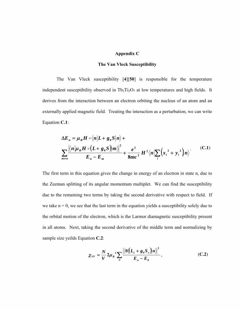
Appendix C

The Van Vleck Susceptibility

The Van Vleck susceptibility [4][50] is responsible for the temperature

independent susceptibility observed in Tb2Ti2O7 at low temperatures and high fields. It

derives from the interaction between an electron orbiting the nucleus of an atom and an

externally applied magnetic field. Treating the interaction as a perturbation, we can write

Equation C.1:

The first term in this equation gives the change in energy of an electron in state n, due to

the Zeeman splitting of its angular momentum multiplet. We can find the susceptibility

due to the remaining two terms by taking the second derivative with respect to field. If

we take n = 0, we see that the last term in the equation yields a susceptibility solely due to

the orbital motion of the electron, which is the Larmor diamagnetic susceptibility present

in all atoms. Next, taking the second derivative of the middle term and normalizing by

sample size yeilds Equation C.2:

( ) ( )∑ ∑≠

++−

+

++=Δ

nm iii

mn

B

Bn

nyxnHmce

EEmSgLHn

nSgLnHE

2222

22

0

0

8μ

μ

. (C.1)

( )∑ −

+=

n n

zzBVV EE

nSgLVN

0

202 0

2μχ , (C.2)

94

which is the Van Vleck susceptibility. Clearly, the Van Vleck susceptibility stems from

electrons switching between different orbital states, or rather between the different crystal

field levels created by the Stark splitting inside of a material. As is the case for Tb2Ti2O7,

if two crystal field levels with different total angular momentum lay close enough that at

low temperatures an applied magnetic field can still excite electrons between them, the

Van Vleck term will yield an apparently temperature independent paramagnetic

susceptibility.

Appendix D

Data on the Stuffed Pyrochlore Tb2(TbxTi2-x)O7-x/2, 0 ≤ x ≤ 0.67

This appendix contains preliminary data taken on the stuffed pyrochlore

Tb2(TbxTi2-x)O7-x/2. Data were taken in the MPMS, PPMS, and dilution refrigerator, and

we used the He3 insert to make the heat capacity measurements.

8.6

8.7

8.8

8.9

9.0

9.1

0 0.1 0.2 0.3 0.4 0.5 0.6 0.7-8.0

-7.5

-7.0

-6.5

-6.0

-5.5

θ W [

K ]

x

Tb2(TbxTi2-x)O7-x/2

T = 7 - 14 K H = 0.1 T

peff [ μ

B / Ln ]

Figure D.1: The Weiss temperature θW and effective moment p as a function of stuffing x in Tb2(TbxTi2-x)O7-x/2. The parameters were obtained from fits on H = 0.1 Tmagnetization data to the Curie Weiss law, over T = 7 – 14 K. (These data were taken by M.L. Dahlberg.)

96

0 1 2 3 4 5 6 70

1

2

3

4

5

Tb2.67Ti1.33O6.67

T = 2 K

M [

μ B /

Tb

]

H [ T ]

Figure D.2: Magnetization versus field data on Tb2.67Ti1.33O6.67 at T = 2 K. (These data were taken by M.L. Dahlberg.)

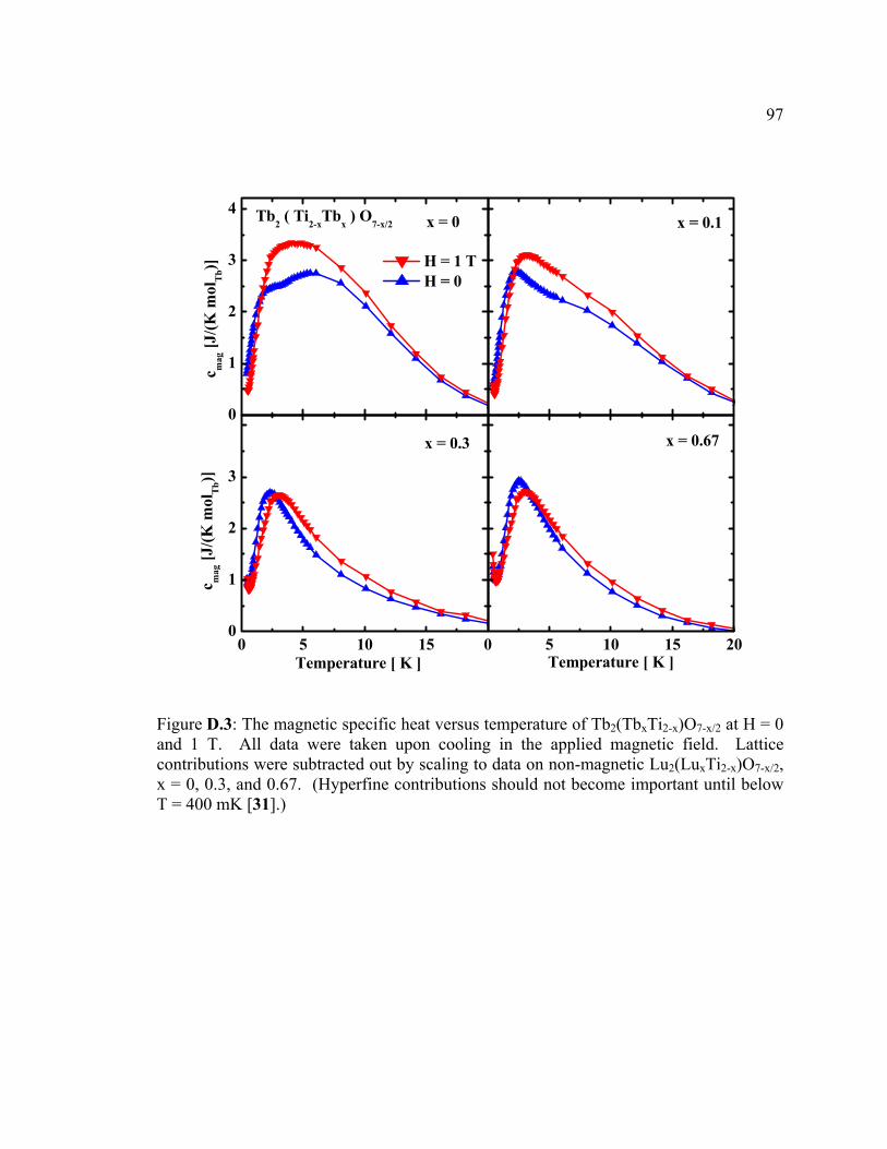
97

0

1

2

3

4

H = 1 T H = 0

Tb2 ( Ti2-xTbx ) O7-x/2c m

ag [J

/(K m

olT

b)]x = 0

x = 0.1

0 5 10 150

1

2

3

x = 0.3

c mag

[J/(K

mol

Tb)]

Temperature [ K ]0 5 10 15 20

x = 0.67

Temperature [ K ]

Figure D.3: The magnetic specific heat versus temperature of Tb2(TbxTi2-x)O7-x/2 at H = 0 and 1 T. All data were taken upon cooling in the applied magnetic field. Latticecontributions were subtracted out by scaling to data on non-magnetic Lu2(LuxTi2-x)O7-x/2, x = 0, 0.3, and 0.67. (Hyperfine contributions should not become important until belowT = 400 mK [31].)

98

0 0.5 1.0 1.5 2.0 2.5 3.01.0

1.2

1.4

1.6

1.8

2.0

2.2

0 5 10 15 200

1

2

3

Tb2(Ti2-xTbx)O7-x/2 H = 0c m

ag /

T [

J / (

K2 m

olT

b )]

Temperature [ K ]

x = 0 0.1 0.2 0.3 0.67

Figure D.4: The magnetic specific heat divided by temperature versus temperature ofTb2(TbxTi2-x)O7-x/2 at H = 0. Lattice contributions were subtracted out by scaling to data on non-magnetic Lu2(LuxTi2-x)O7-x/2, x = 0, 0.3, and 0.67. (Hyperfine contributionsshould not become important until below T = 400 mK [31].)

99

0 0.5 1.0 1.5 2.0 2.5 3.00.6

0.8

1.0

1.2

1.4

1.6

1.8

2.0

2.2

0 5 10 15 200

1

2

3 Tb2(Ti2-xTbx)O7-x/2 H = 1 T

c mag

/ T

[ J

/ ( K

2 mol

Tb )]

Temperature [ K ]

x = 0 0.1 0.2 0.3 0.67

Figure D.5: The magnetic specific heat divided by temperature versus temperature ofTb2(TbxTi2-x)O7-x/2 at H = 1 T (field cooled). Lattice contributions were subtracted out byscaling to data on non-magnetic Lu2(LuxTi2-x)O7-x/2, x = 0, 0.3, and 0.67. (Hyperfine contributions should not become important until below T = 400 mK [31].)

100

0 4 8 12 16 20 24 28 320

1

2

3

4

5

6

7

8

x = 0 0.1 0.2 0.3 0.67

R ln 2.5

Tb2(Ti2-xTbx)O7-x/2 H = 0

R ln 2

R (ln 2 - 0.5 ln 1.5)

S [ J

/ (m

olT

b K )]

Temperature [ K ]

Figure D.6: The integrated magnetic entropy versus temperature of Tb2(TbxTi2-x)O7-x/2 at H = 0. Lattice contributions were subtracted out by scaling to data on non-magnetic Lu2(LuxTi2-x)O7-x/2, x = 0, 0.3, and 0.67.

101

0 4 8 12 16 20 24 28 320

1

2

3

4

5

6

7

8

x = 0 0.1 0.2 0.3 0.67

R ln 2.5

Tb2(Ti2-xTbx)O7-x/2 H = 1 T

R ln 2

R (ln 2 - 0.5 ln 1.5)

S [ J

/ (m

olT

b K )]

Temperature [ K ]

Figure D.7: The integrated magnetic entropy versus temperature of Tb2(TbxTi2-x)O7-x/2 at H = 1 T (field cooled). Lattice contributions were subtracted out by scaling to data onnon-magnetic Lu2(LuxTi2-x)O7-x/2, x = 0, 0.3, and 0.67.

102

0 0.5 1.0 1.5 2.00

0.2

0.4

0.6

0.8

1.0

1.2

0 5 10 15 200

0.4

0.8

1.2

Tb2.67Ti1.33O6.67 H = 0

χ′ [

emu

/ Oe

mol

Tb ]

T [ K ]

f = 10 Hz 50 Hz 100 Hz 500 Hz 1 kHz

χ′ [

emu

/ Oe

mol

Tb ]

T [ K ]

Figure D.8: The real part of the H = 0 AC susceptibility of Tb2.67Ti1.33O6.67 versus temperature for various measurement frequencies. Open symbols represent data taken in the ACMS, while closed circles represent data taken in the dilution refrigerator. Thesedata were calibrated assuming χ′(H = 5 T, T = 1.8 K) = 0 (see Section 3.5.3).

103

0 0.5 1.0 1.5 2.0 2.5 3.0 3.5 4.0 4.5 5.00

0.2

0.4

0.6

0.8

1.0

1.2

χ′ [

emu

/ (O

e m

olT

b) ] "Field Cooled" T = 1.8 K 0.001T/min "Field Cooled" T = 1.5 K 0.001T/min "Field Cooled" T = 0.5 K 0.001T/min "Field Cooled" T = 0.2 K 0.001T/min "Zero Field Cooled" T = 0.2 K 0.01T/min

Tb2.67Ti1.33O6.67 f = 50 Hz

H [ T ]

Figure D.9: The real part of the f = 50 Hz AC susceptibility of Tb2.67Ti1.33O6.67 versus field at various temperatures, and field sweeping rates. These data were calibratedassuming χ′(H = 5 T, T = 1.8 K) = 0 (see Section 3.5.3).

104

0.0 0.2 0.4 0.6 0.8 1.00.46

0.48

0.50

0.52

0.54

0.56

0.58

0.60

0.62

0 1 2 30

0.2

0.4

0.6

Zero Field CooledField Cooled

Zero Field Cooled

T = 0.3 K T = 0.2 K

χ′ [

emu

/ (O

e m

olT

b) ]Tb2.67Ti1.33O6.67 f = 50 Hz

H [ T ]

Field Cooled

H [ T ]

χ′ [

emu

/ (O

e m

olT

b) ]

Figure D.10: The real part of the f = 50 Hz AC susceptibility of Tb2.67Ti1.33O6.67 versus field at T = 0.3 K and 0.2 K, taken after initially zero field cooling or field cooling thesample. These data were calibrated assuming χ′(H = 5 T, T = 1.8 K) = 0 (see Section 3.5.3).

VITA

Benjamin George Ueland

Education: M.S. Physics Binghamton University 2001 Advisor: Robert L. Pompi B.A. Physics Binghamton University 2000 Selected Publications: J. W. Snyder, B. G. Ueland, J. S. Slusky, H. Karunadasa, R. J. Cava, A. M. Mizel

and P.Schiffer, “Quantum-Classical Reentrant Relaxation Crossover in Dy2Ti2O7 Spin Ice”, Phys.Rev. Lett. 91, 107201 (2003).

Z. Mao, T. He, M. M. Rosario, K. D. Nelson, D. Okuno, B. G. Ueland, I. G.

Deac, P. Schiffer, Y. Liu and R. J. Cava, “Quantum phase transition in quasi-one-dimensional BaRu6O12”, Phys. Rev. Lett. 90, 186601 (2003).

J. W. Snyder, B. G. Ueland, J. S. Slusky, H. Karunadasa, R. J. Cava and P.

Schiffer, “Low temperature spin freezing in the Dy2Ti2O7 spin ice”, Phys. Rev. B 69, 064414 (2004).

B. G. Ueland, P. Schiffer, R. E. Schaak, M. L. Foo and V. L. Miller, “Specific

heat study of the Na0.3CoO2 DT 1.3H2O superconductor: influence of the complex chemistry”, Physica C 402, 27-30 (2004).

B. G. Ueland, G. C. Lau, R. J. Cava, J. R. O’Brien and P. Schiffer, “Slow Spin

Relaxation in a Highly Polarized Cooperative Paramagnet”, Phys. Rev. Lett. 96, 027216 (2006).

G. C. Lau, R. S. Freitas, B. G. Ueland, B. D. Muegge, E. L. Duncan, P. Schiffer

and R. J. Cava, “Zero-point entropy in stuffed spin-ice”, Nat. Phys. 2, 249–253 (2006). A. Olariu, P. Mendels, F. Bert, B. G. Ueland, P. Schiffer, R. F. Berger, and R. J.

Cava, "Unconventional Dynamics in Triangular Heisenberg Antiferromagnet NaCrO2,", Phys. Rev. Lett. 97, 167203 (2006).