CONVERGENCE PROPERTIES of

FRACTIONALLY-SPACED EQUALIZERS for

DATA TRANSMISSION

M. Melih Pekiner, B.Sc. Bogazi& Uraiuersity, Istanbul

Department of Electrical Engineering

A thesis submitted to the Faculty of Graduate Studies and Research

in partial fulfillment of the requirements for the degree of

Master of Engineering

Department of Electrical Engineering Mc Gill University Montreal, Canada

August 1982

ABSTRACT

This thesis considers the convergence properties of adaptive equalizers used

for data transmission. In the conventional form of a tapped delay line equalizer,

the tap spacing is equal to the symbol interval T. Two other cases are discussed.

The fractional-spaced equalizer has tap spacing less than T ( T / 2 ie considered in

detail). A hybrid configuration uses both T spaced and fractional T spaced tap is also

considered. From the mathematical derivations and the computer simulations the

properties, the relative advantages and drawbacks of the three cases are analysed.

Cette thkse traite des propri6txh de convergence des kgaliseurs conventionnels

dims le domaine des transmissions de donnhes. Dam un Bgaliseur conventionnel la

distance entre perforations correspond l'intervalle entre symboles T. Deux autres

configurations sont ici considdr6s: 1'6galiseur B espace fractionnel dont la distance

entre perforations est infhrieure B T, et l'dgaliseur hybride, utilisant des distances

de perforation dgales B T et inferieures B T. Lee di6rentes propri6ths, avantages et

inconv6nients des trois types d'6galiseurs sont compar6s sur une baie mathbmatique

et de simulation par ordinateur.

ACKNOWLEDGEMENTS

I wish to extend my sincere thanks to Dr. P. Kabal for his! guidance, and

constant support in every aspect of this work; to Dr. M. Ferguson for hi help in the

docu.mentation, to K. Gupta for his help in going over the text; to Dr. Y. Youssef

and A. Dill for their help in creating some of the figures in this thesis; to Miss

J. Chardon for her translation of the abstract; and to the Marauders for the very

friendly atmosphere they have created in the o%ce and in the computer labaratory.

And to my parents for their encouragement, financial support and continuing

interest in my academic progress.

TABLE of CONTENTS

.. Abfitract . . . . . . . . . . . . . . . . . . . . . . . . . . . . . . . . . . . . . u

Resum8 . . . . . . . ; . . . . . . . . . . . . . . . . . . . . . . . . . . . . iii

Acknowledgements . . . . . . . . . . . . . . . . . . . . . . . . . . . . . . . iv

Table of Contents . . . . . . . . . . . . . . . . . . .' . . . . . . . . . . . . vi

List of Figures . . . . . . . . . . . . . . . . . . . . . . . . . . . . . . . . . ix CHAPTER I INTRODUCTION . . . . . . . . . . . . . . . . . . . . . . 1

1.1 ADAPTIVE EQUALIZATION . . . . . . . . . . . . . . . . . . . . . .1 1.2 THESIS OVERVIEW . . . . . . . . . . . . . . . . . . . . . . . . . . . 3

CHAPTER 11 BASEBAND DIGITAL DATA COMMUNICATION SYSTEM 4

II.1 MODEL of DIGITAL COMMUNICATION SYSTEM . . . . . . . . . . 4

II.2 INTERSYMBOL INTERFERENCE and WHITE NOISE . . . . . . . - 7

CHAPTER I11 OPTIMAL MINIMUM MEAN-SQUARE ERROR

EQUALIZATION . . . . . . . . . . . . . . . . . . . . . . . . . . . . . . . 10

III.2 CRITERIA for OPTIMAL RECEM3R DESIGN . . . . . . . . . . . 16

- -

CHAPTER lV PROPERTIES of T.T/ %SPACED

. . . . . . . . and HYBRID TRANSVERSAL EQUALIZERS 26

. . . . . . . . . . . . . . . . rV.1 IMPLEMENTATION of EQUALIZERS 26

. . . . . . . . . . . . . N . 2 PROPERTIES OF T SPACED EQUALIZER 28

. . . . . . . . . . N.2.1 The Autocovariance Matrix and Its Eigenvalues 28

. . . . . . . . . . . . . . N.2.2 The Frequency Response of the Equalizer 29

. . . . . N.2.3 The Minimum Mean Square Error of an Infinite Equalizer 30

. . . . . . . . . . . . . N . 3 PROPERTIES o~T/~-SPACED EQUALIZER 31

. . . . . . . . . . . . IV.3.1 The Frequency Response of the T/2 Equalizer 31

. . . . . . . . . . . IV.3.2 The Autocovariance Matrix and Its ~ i~enva lues 33

N.3.3 The Minimum Mean-Square Error of an Infinite Equalizer . . . . . 34

. . . . . N . 4 PROPERTIES of HYBRID TRANSVERSAL EQUALIZER 35

. . . . . . . . . . . . . IV.4.1 The Optimal Hybrid Transversal Equalizer 35

CHAPTER V CONVERGENCE PROPERTIES of the

. . . . . . . . . . . . . . . . TRANSVERSAL EQUALIZERS 39

V.1 THE RECURSnrE ALGORITHMS for COMPUTING the TAP GAINS . 39

. . . . . . . . . . . . . V.2 THE STEEPEST DESCENT ALGORITHM 42

. . . . . . . . . . . . . . . . . . . . . . . . . V.2.1 Performance Surface 42

. . . . . . . . . . . . . . . . . . . . . V.2.2 Coordinate Transformation 45

. . . . . . . . . . . . . . . . . . V.2.3 Convergence Properties of h and c 47

V.3 EXCESS MEAN-SQUARE ERROR (ea) . . . . . . . . . . . . . . . . 50

- G -

CHAPTER VI RESULTS . . . . . . . . . . . . . . . . . . . . . . . . 52

VI.1 DESCRIPTION of the SIMULATION . . . . . . . . . . . . . . . . . 52

. . . . . . . . . . . . . . . . . VI.2 COMPARISON of the EQUALIZERS 55

. . . . VI.2.1 On the Convergence of the TSpaced, ~/f-Spaced and HTEs 60

. . . . . . . . . VI.3 THE EXCESS-MSE(eA) and the STABILITY LIMITS 63

. . . . . . . . . . . . . . . VI.3.1 Minimum MSE Versus Number of Taps 63

. . . . . . . . . . VI.3.2 Effects of Step Size on Excess-MSE and Stability 65

SUIJIMARY and CONCLUSION . . . . . . . . . . . . . . . . . . . . . . . 69

LITERATURE . . . . . . . . . . . . . . . . . . . . . . . . . . . . . . . . 71

APPENDIX . . . . . . . . . . . . . . . . . . . . . . . . . . . . . . . . . . 74

. A.1 The Derivation of Eq [3.16] . . . . . . . . . . . . . . . . . . . . . . . . 74

A.2 The Derivation of Eq . [3.20] . . . . . . . . . . . . . . . . . . . . . . 76

. A.3 The Derivation of Eq [3.25] . . . . . . . . . . . . . . . . . . . . . . 77

. . . . . . . . . . . . . . . . . . . . . . . . . . A.4 Proof of Theorem 1 78

LIST of FIGURES

Fig . No . . . . . . . . . . . . . . . . . . . 2.1 Structure of a Coxhmication System 5

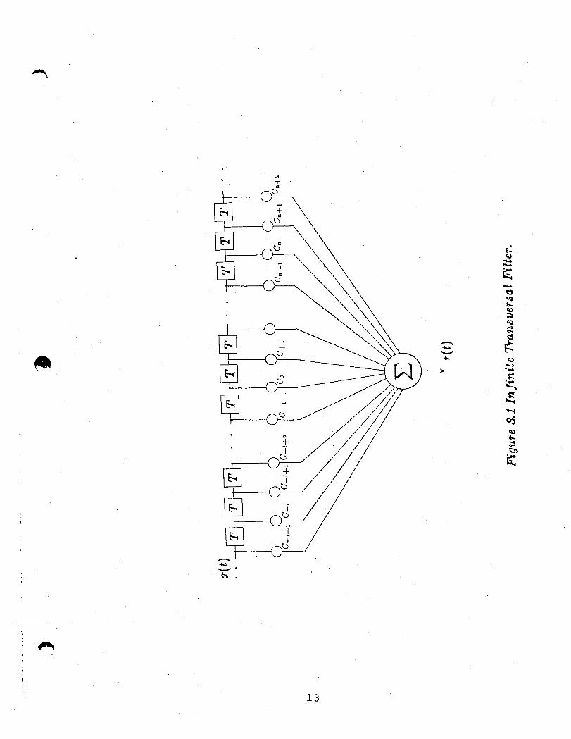
. . . . . . . . . . . . . . . . . . . . . . . . 3.1 InGnitenansversalFilter 13

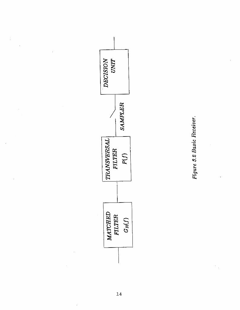
. . . . . . . . . . . . . . . . . . . . . . . . . . . . . 3.2 Basic Receiver : 14

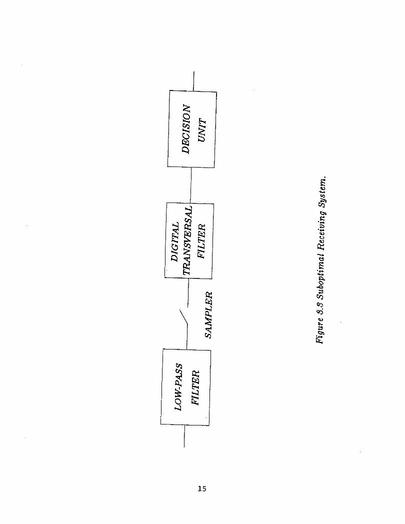
. . . . . . . . . . . . . . . . . . . . . 3.3 Suboptimal Receiving System 15

. . . . . . . . . . . . . . . . . . . . . . . . . . 3.4 Generalized Equalizer 17

. . . . . . . . . . . . . . . . . . . . . . . 3.5 Generation of Error Signal 21

. . . . . . . . . . . . . . . . . . 4.1 Hybrid Transversal Equalizer Model 37

. . . . . . . . . . . . . . . . . . . . . . . . . . 5.1 Performance Surface 43

. . . . . . . . . . 5.2 Feedback Model for the Tap Coefficient Adjusment 46

6.1 Sampled and Interpolated Impulse Responses of

. . . . . . . . . . . . . . . . . . . . Simulated Transmission Channels 54

6.2 Minimum Achievable MSE versus Time Span of the Filter . . . . . . 58 . . . . . . . . . . . . . . . 6.3 MSE Limits vs Additional Tap Placement 59 .

6.4 Comparison with one Additional Tap . . . . . . . . . . . . . . . . . 61

- k -

6.5 Comparison of the Three Cases . . . . . . . . . . . . . . . . . . . . 82

6.6 Performance of the T / 2 Equalizer with Different Number of Taps . . . 64

6.7 Performance of the 20 Tap T / 2 Equalizer with Dierent Step Sizes . . 66

6.8 Performance of the 30 Tap T / 2 Equalizer with Dierent Step Sizes . . 67

6.9 Performance of the 40 Tap TI2 Equalizer with Different Step Sizes . . 68

CHAPTER I

INTRODUCTION

1.1 Adaptive Equalization

Digital data transmission systems are often bandwidth limited. Moreover, the

channel characteristics may change for each transaction or even during transactions.

The recent applications of computer communication on the voice-bandwidth chan-

nels, and satellite channels has raised a new interest in the optimization of data

transmission systems.

The transmission channel tends to degrade the transmitted signal, causing

difficulties in recovering the original data. One of the sources of degradation is the

additive noise due to background thermal noise or impulsive noise. This noise can

be reduced to some extent by using bandpass filters to exclude out-of-band noise.

Another form of degradation is the time dispersion, which extends the duration of

the input signal, causing the adjacent data symbols to interfere with each other.

This effect of overlapping of received symbols is called Intersymbol Interference (ISI)

[R.W. Lucky, J. Salz and E.J. Weldon, 19681.

- 1 -

Bandwidth efficient data transmission over the real analog channels requires

equalization to reduce intersymbol interference. The idea behind equalization is to

reduce the cross effects between the individual symbols using the past and the future

samples. In practice, the equalizer is implemented in the form of a transversal filter

or a tapped delay line. The weighted outputs of the delay taps are summed to form

the output of the filter. An automatic or adaptive equalizer varies these tap weights

by using one of the methods described in [Gersho, 19691, [Hirsch, 19701, [Lucky,

1965, 19671, [Chang, 19711.

There are two basic kinds of adjusment procedures. The first one, often called

automatic equalization, is done by sending a string of isolated test pulses before

the actual data is transmitted. The equalizer tap coefficients are kept constant after

this 'training' period. In the other method, 'adaptive equalization', the equalizer

settings are updated directly from the received data. Adaptive equalizers minimize

the degradation of the signal using, first the a prion' known training sequence, and

then an estimate of the data during transmission. When actual data transmission

starts, the distortion is already reduced to a small value. At this moment, the

equalizer can use the reconstructed output signal of the receiver as a reference

signal. This k i d of operation is usually referred to as decision-directed mode. The

effect of wrong decisions is usually negligible after a successful training period.

Early equalizers used a tap spacing of T, the symbol spacing period. Recent,

studies on equalizers showed that further improvement in performance can be ob-

tained using a tap time spacing of less than T. These equalizers that have tap spacing

less than T are called F'ractional-Tap-Spaced-Equalizers. This type of equalizer has

been analysed by [Ungerboeck, 19761, [Gitlin and Weinstein, 19811, [Qureshi and

Forney, 19771.

In digital data communication systems, not only are different channels used

- 2 -

each time a transmission is requested, but the channel itself may have time varying

characteristics. A data transmission is made up of a training period which is followed

by the transmission of the actual data. The start-up time is defined as the time

during which the receiver locks on to the carrier, establishes bit synchronization

and performs automatic equalization. This overhead takes a considerable portion of

the total busy period. For the early automatic equalizers, settling times in the order

of seconds have been reported. Since then great improvements have been achieved.

1.2 'Thesis Overview

In this work, we study the adaptation behaviour of conventional, fractional-

spaced, and hybrid equalizers. The idea of a hybrid equalizer was first proposed by

P. Kabal and studied by [Nattiv, 19801.

The second chapter describes a baseband digital data communication system

using passband equivalent model for the system to be studied. The problem of in-

tersymbol interference is also discussed. The following chapter consists of an over-

view of optimal minimum mean-square error equalization. Chapter 3 also includes a

study of an equalizer analysis with general tap spacing. In Chapter 4, the properties

of the conventional, fractional-tap spaced, and hybrid equalizers are discussed ,in

terms of their frequency characteristics, eigenvalues and minimum mean-square er-

ror. Chapter 5 starts by introducting algorithms used for the adaptive equalizers.

This is followed by a summary of the steepest descent algorithm for tap adjust-

ments. The chapter concludes with the discussion on the convergence properties of

the equalizers. The description of the simulation and the results are presented in

Chapter 6.

CHAPTER n BASEBAND DATA COMMUNICATION SYSTEM

11.1 Model of Digital Communication System

The structure of a digital communication system can be modelled as in Figure

2.1. The three main blocks are the transmitter, the channel and the receiver.

The source symbols a t every T second intervals are passed through a bandlimited

filter whose impulse response is h,(t), and g~( t ) is generated a t the output of the

transmitter,

This signal is fed tb the channel which is viewed as a filter of impulse response

h,(t). Random noise n,(t) is added by the channel and the final form of the signal

is,

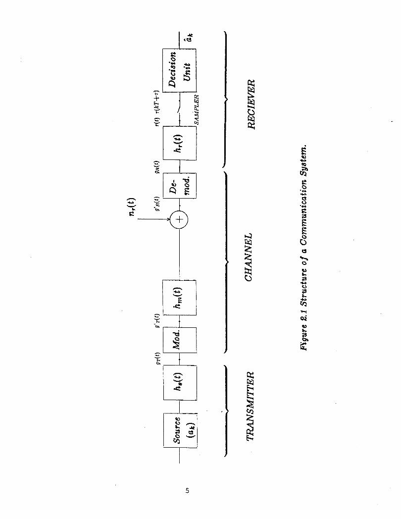
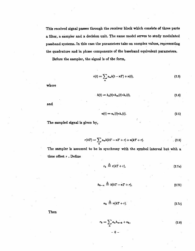
This received signal passes through the receiver block which consists of three parts

a filter, a sampler and a decision unit. The same model serves to study modulated

passband systems. In this case the parameters take on complex values, representing

the quadrature and in phase components of the baseband equivalent parameters.

Before the sampler, the signal is of the form,

and

The sampled signal is given by,

r(kT) = a , h ( k ~ - nT + r) + n(kT + 7). (2.6) n

The sampler is assumed to be in synchrony with the symbol interval but with a

time offset r . Define

A rk = r(kT + r),

A hk-, = h(kT - nT + r),

Then

are the samples input at .the decision unit. The sampling time is offset by r with

respect to source clock. The final; block outputs a symbol & which is an estimate

of the input at the source.

When one starts to look at optimizing the above system, the approach might be

either to optimize the transmitter or the receiver, or both, if enough knowledge is

available about the system. In general, the receiver is optimized in order to improve

the mean-square error, output Signal-to-Noise Ratio (SNR), probability of error etc.

Thia can be achieved with some improved designs of receiver filter and decision unit.

In this work, we study the receiver when the channel characteristics are unknown

a t the receiver end. Our approach is to minimize the mean-square error, thus to

reduce the effect of both intersymbol interference and noise.

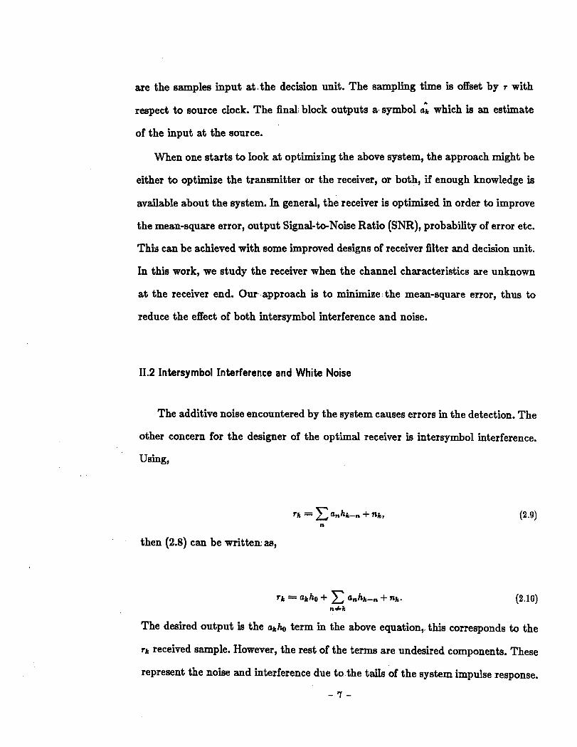
11.2 Intersymbol Interference and White Noise

The additive noise encountered by the system causes errors in the detection. The

other concern for the designer of the optimal receiver is intersymbol interference.

using,

then (2.8) can be written; as,

The desired output is the akhO term in the above equation,. this corresponds to the

rk received sample. However, the rest of the terms are undesired components. These

represent the noise and interference due tothe tails of the system impulse response.

This interference due to past and: future samples of h(t) a t the sampler output are

referred to as the Intersymbol Interference (ISI).

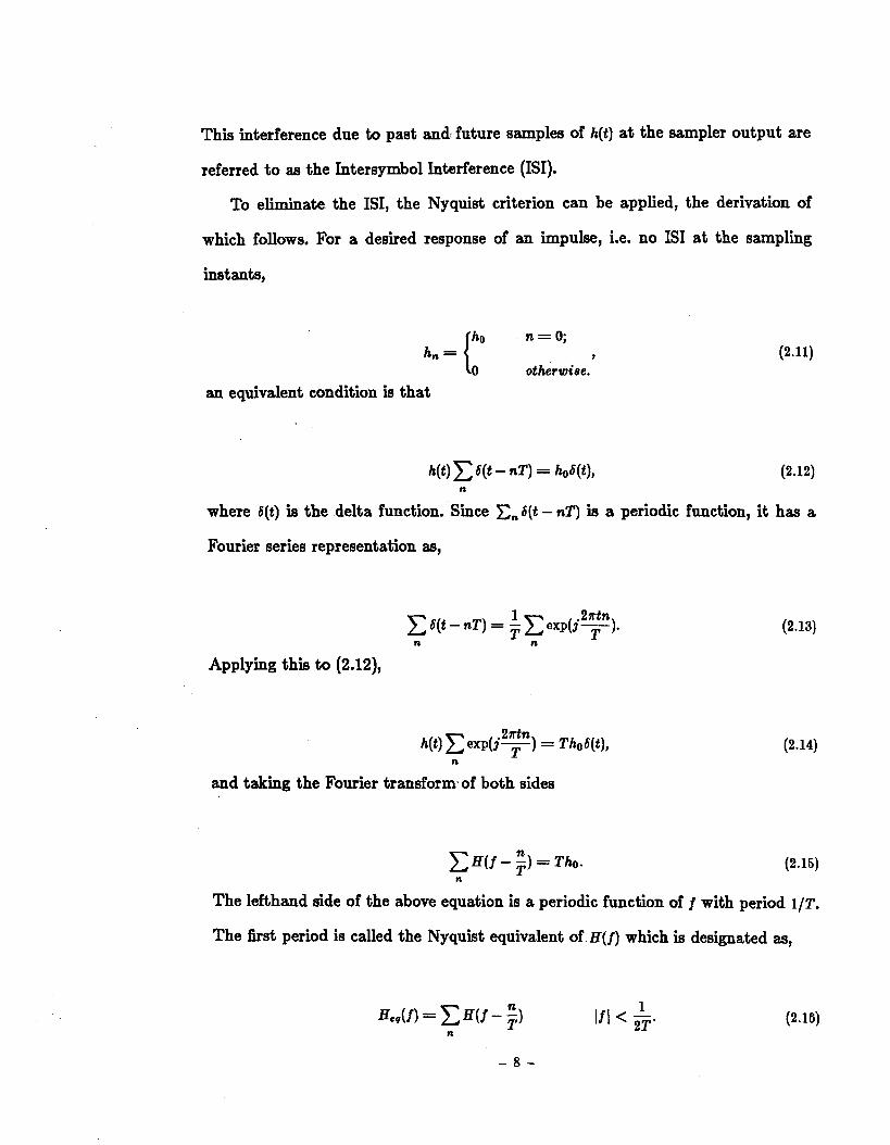
To eliminate the ISI, the Nyquist criterion can be applied, the derivation of

which follows. For a desired response of an impulse, i.e. no IS1 at the sampling

instants,

ho n = 0; hn= { 8

0 otherwiee.

an equivalent condition is that

h(t) 6(t - nT) = ho6(t), (2 .12) n

where S(t) is the delta function. Since En 6( t - nT) is a periodic function, it has a

Fourier series representation as,

Applying this to (2.12),

and taking the Fourier transform of both sides

The lefthand side of the above equation is a periodic function of f with period 1/T.

The first period is called the Nyquist equivalent of H ( f ) which is designated as,

It can eady be observed that for the elimination of intersymbol interferance &,(I)

should be flat. This amounts to the requirement that at each sampling instant all

h,'s be zero except ho.

CHAPTER m OPTIMAL MINIMUM MEAN SQUARE ERROR EQUALIZATION

111.1 Structure of Optimum Receiving Filter

In this chapter, the structure! of the receiver is discussed and an optimization

analysis is carried out. The possible criteria to optimize the receiver are introduced,

and one selected, namely minimization of the mean-square error.

For a receiver structure as in Figure 2.1, which has a receiving filter, a detector

and a decision unit, Ericson proposed a model which performs at least as well

as any other filter. He shows that the optimum linear filter can be decomposed

into two parts, a matched filter and a periodic filter. The former is a filter of the

same bandwidth. as that of the channel, while the:latter can be implemented as a

transversal filter. Then

for

and P(f) is periodic with period 112'. Hr(f), the receiver input filter performs at least

as well as any other linear filter for the minimization of intersymbol interference,

signal-to-noise ratio, andlerror probabilty criterion.

The periodic frequency response of P ( j ) can be represented by an infinite analog

transversal filter. Such a filter is shown in Fig. 3.1. Based on the above result, the

receiver of a basic communication system can be shown as in Figure 3.2.

The term Hm*(f)/Qnm(f) is the frequency response of the filter which is matched

to the signal waveform. This structure can be summarized as follows: the matched

filter maximizes the signal-to-noise ratio a t the decision instant, while the transversal

filter P(f), reduces the intersymbol interference that still corrupts the signal in its

input.

Havever, the above receiver model is impractical due to the following reasons;

(i) An infinite length transversal filter cannot be realized. (ii) Since the channel

characteristics are assumed to be unknown, each time a connection is made, it is

impractical to realize a matched filter (or even when the same channel is used and

the channel itself slowly changes in time).

In practice, only a cascade of a lowpass filter and a transversal filter is used.

Another simplification in the implementation is to place the sampler in Figure 3.3

before the transversal filter (to keep the samples in digital form for use in the

calculation of the optimum tap coefficients). This reduces the transversal filter to

a shift register. The adaptation procedure can then be performed digitally. One

more point is that the transversal filter can be used to minimize the intersymbol

interference by forcing the overall response H(f) to obey (2.14). This causes the

Nyquist equivalent channel to be flat. The name equalizer is given for that reason.

The final form of the suboptimal.digital receiving end is summarized as in Figure

3.3.

111.2 Criteria for Optimal Receiver Design

To design the receiver, one must first come up with a receiver structure. Then,

given this structure, the filter H ( j ) can be optimized. But, due to intersymbol

interference, there are several different optimization criteria. One of them is to try to

minimize the error probabilty resulting from the noise and intersymbol interference,

but this approach leads to quite intractable calculations. To obtain the solution,

one has to solve a set of complicated nonlinear simultaneous equations. A much

simpler approach, is to eliminate the intersymbol interference, and then minimize

the error probability subject to some constraint. Maximizing the signal-to-noise

ratio at the sampling instants can also be used as another optimization criterion.

The equalization is achieved by finding a set of gains for the equalizer taps. These

tap coefficients can be put in a vector form, (*)

where there are Nl taps to the left, N2 taps to the right of the reference tap (see

Figure 3.4). The values of these taps are chosen so as to minimize the mean-square

error between the output.of the data source and output of the decision unit in the

receiver. In the next section, the optimization problem is solved for a generalized

equalizer in which the spacing between the taps is arbitrary. The special cases to

be studied are derived from this model.

[.IT ia the trampone of the vector;

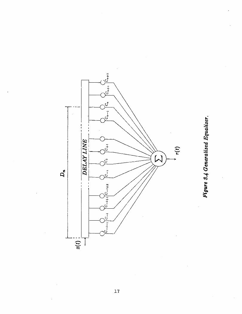
111.3 Generalized Optimal Mean Square Error Equalizer

The generalized equalizer with arbitrary tap spacing is shown in Figure 3.4.

Using an analog version of the equalizer (a tapped delay line) with a continuous

signal at its output,

For arbitrary spacing; DjT of tap spacings then, the output of the equalizer can

be written as:

The p h tap has a delay of DjT associated with itself. The above output is then

sampled a t symbol intervals. The output of the sampler feeds the following signal

to the decision unit

y(kT + r) = e j z(kT - DjT + r), (3.8) i

where r is the sampling time offset with respect to source clock. Using the vector

notation:

where: 5 is the vector of the tap coefficients;

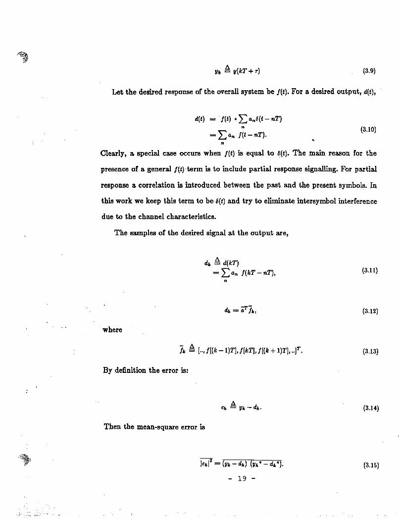
Let the desired response of the overall system be j(t). For a desired output, d(t),

Clearly, a special case occurs when j(t) is equal to 6(t). The main reason for the

preoence of a general j(t).term is to include partial response signalling. For partial

response a correlation is introduced between the past and the present symbols. In

this work we keep this term to be:6(t) and try to eliminate intersymbol interference

due to the channel characteristics.

The samples of the desired signal at the output are,

where

By definition the error is:

Then the mean-square error is

rn = (Ilk - 4) ( ~ k * - dk*).

- 19 -

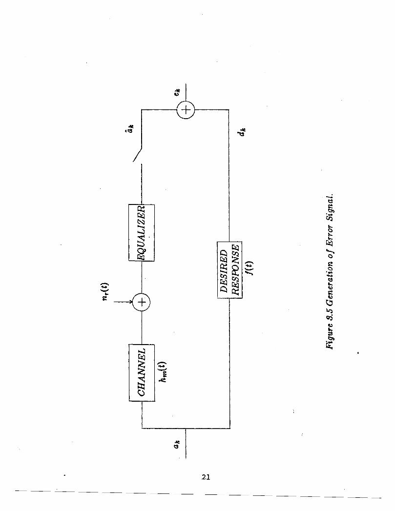
The above expectation is over the sample space ah. The block diagram for the

generation of the error signal is shown in Figure 3.5.

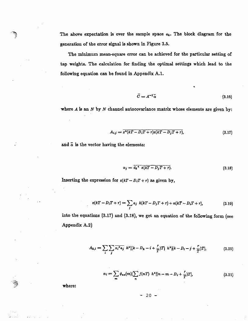
The minimum mean-square error can be achieved for the particular setting of

tap weights. The calculation for: finding the optimal settings which lead to the

following equation can be found in Appendix A.1.

where A is an N by N channel autocovariance matrix whose elements are given by:

Acj = z*(kT - DiT + r)z(kT - DjT + r ) ,

and iE is the vector having the elements:

aj = dk* z(kT - DjT + r ) .

Inserting the expression for z(kT - DiT + r ) as given by,

t(kT - DiT + 7 ) = C aj h(kT - DjT + 7 ) + n(kT - DiT + T), (3.19) i

into the equations (3.17) and (3.18), we get an equation of the folIowing form (see

Appendix A.2)

where:

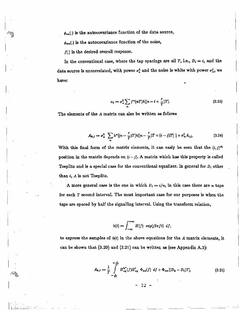
#,(.) is the autocovariance function of the data source,

#,,(.) is the autocovariance function of the noise,

f(.) is the desired overall response.

In the conventional case, where the tap spacings are all T, i.e., Di = i , and the

data source is uncorrelated, with power uz and the noise is white with power a:, we

have: L

The elements of the A matrix can also be written as follows

With this final form of the matrix elements, it can easly be seen that the ( i , j)th

position in the matrix depends on (i - j). A matrix which has this property is called

Toeplitz and is a special case for the conventional equalizer. In general for Di other .

than i , A is not Toeplitz.

A more general case is the one in which Di = i /n , in this case there are n taps

. . for each T second interval. The most important case for our purposes is when the

taps are spaced by half the signalling interval. Using the transform relation,

to express the samples of h(t) in the above equations for the A matrix elements, it

can be shown that (3.20) and (3.21) can be written as (see Appendix A.3):

where

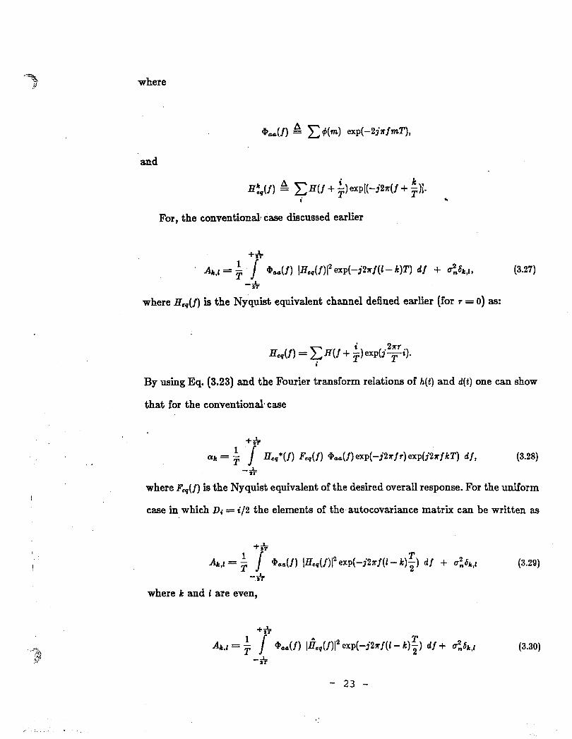
For, the conventional: case discussed earlier

Q,U) I H . , ( ~ ) 1 2 e x p ( - j W (i - LIT) df + & 5 0 , 1 , (3.27)

-I 1T

where H.,(f) is the Nyquist equivalent channel defined earlier (for s = 0) as:

By using Eq. (3.23) and the Fourier transform relations of h(t) and d(t ) one can show

that for the conventional. case

++ a = ' T ' / aeq*(f) ~ . , ( j ) aa(f) e x p ( - j ~ r f r ) e x p ( j k k ~ ) d f , (3.28)

-1 1T

where F,,( f ) is the Nyquist equivalent of the desired overall response. For the uniform

case in which Di = i / 2 the elements of the- autocovariance matrix can be written as

where k and 1 are even,

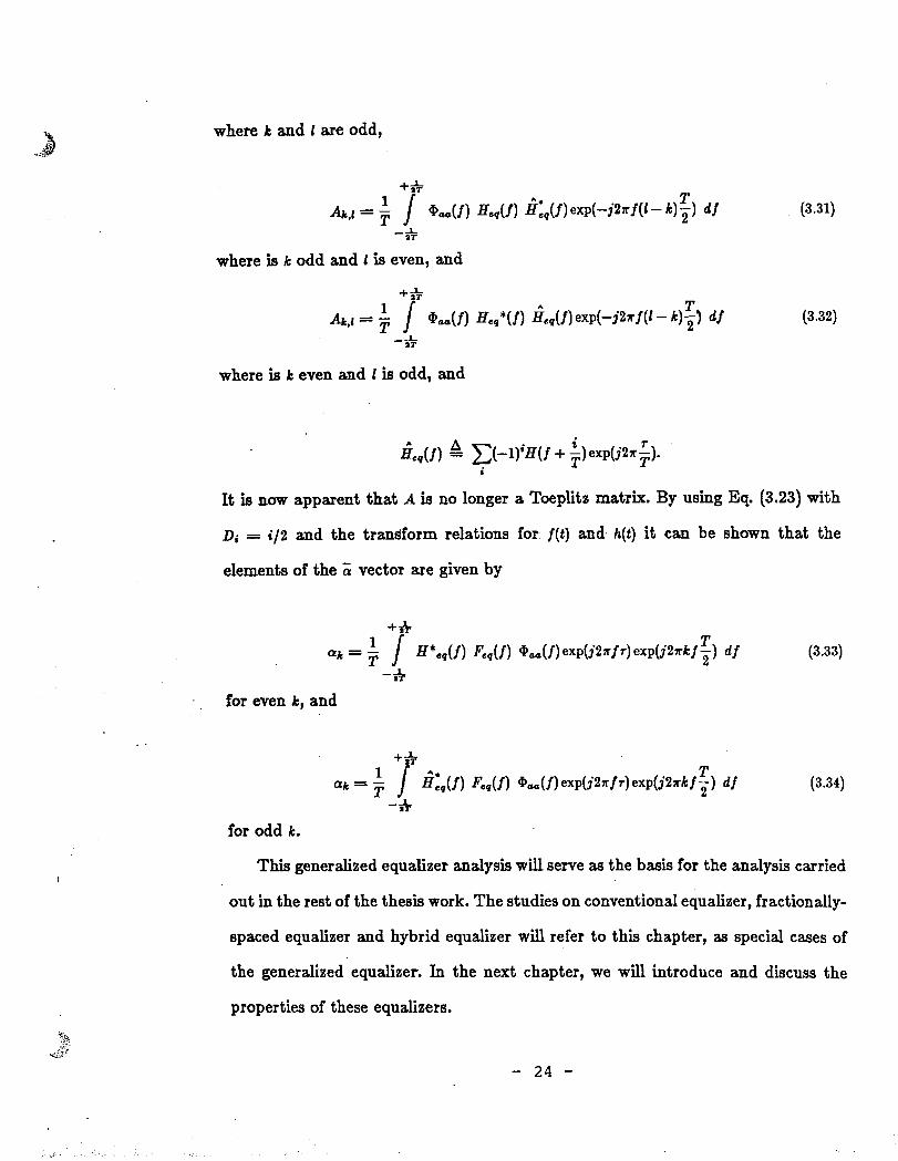
where k and i are odd,

where is k even and i is odd, and

It is now apparent that A is no longer a Toeplitz matrix. By using Eq. (3.23) with

Di = i t 2 and the transform relations for. f ( t ) and h(t) it can be shown that the

elements of the vector are given by

-A for even k, and

Thii generalized equalizer analysis will serve as the basis for the analysis carried

out in the rest of the thesis work. The studies on conventional equalizer, fractionally-

spaced equalizer and hybrid equalizer wiil refer to this chapter, as special cases of

the generalized equalizer. In the next chapter, we will introduce and discuss the

properties of these equalizers.

CHAPTER IV

P'rEOPEEM'IES of T, TJ2-SPACED and HYBRID TRANSVERSAL EQUALIZERS

N.l Implementation of Equalizers

In the previous sections we have mentioned that equalizers are placed at bhe

receiver end as decision-directed adaptive receivers. This chapter discusses the

theory and the implementation techniques as well as the properties of adaptive

equalizers.

For optimum equalization, one has to find the set of tap coefficients to reduce ,

intersymbol interference and noise. The solution (3.16) involves the inversion of the

N x N A matrix, where N , the total number of taps may be quite large. Iterative

methods for solving Eqn. (3.16) will be discussed in the next chapter.

The hardware implementation of the adaptive equalizers can be classified into

the following categories: analog, hardwired digital and programmable digital.

Early implementations used analog tapped delay lines, made up of indnctor-

capacitor (LC) and switched ladder attenuators as tap gains. Field-effect transistors

later replaced the switched attenuators. As the technology became available, digi-

- 26 -

tal implementations were introduced, offering reduced size and increased accuracy.

More recently, large-scaled integrated (LSI) analog implementations based on the

charge-coupled device (CCD) technology renewed the interests in analog techniqucs.

In this technique the sampled input waveform is stored and transferred as con-

tinuous-valued charge packets. The variable tap gains are stored in digital form,

and the multiplication of the tap gains and the samples are done using a multiply-

ing digital-to-analog converter. This method is still to be implemented, but it haa

significant potential in applications where the symbol rates are high enough to make

the digital versions impractical or very costly.

The other class, namely the hardwired digital technology which was the most

commonly used during the past decade. The input signal is used in sampled and

digitized form, suitable for storing in the registers. The tap gains were stored in the

digital shift registers as well. The formation and accuinulation of products takes

place in logic circuits connected to perform digital arithmetic.

The most recent advance in the field is the application of programmable digi-

tal signal processors. In this type of implementation the equalization function is

performed in a series of steps or instructions in a microprocessor or a digital com-

putation structure specially built to efficiently perform the type of digital arithmetic

required. The same hardware can then be time-shared to perform functions such .as

filtering, modulation and demodulation in a modem. The greatest advantage of this

technology is that it is flexible, and permits sophisticated equalizer structures and

training procedures to be implemented with ease.

IV.2 Properties of T-spaced Equalizer

IV.2.1 The Autoeovarlanee Matrix and i ts Elgenvalues

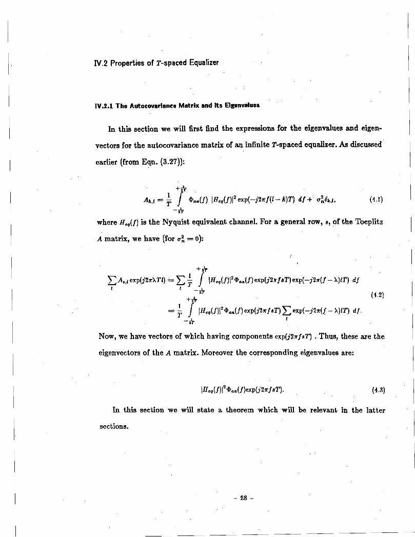
In this section we will first find the expressions for the eigenvsluea and eigen-

vectors for the autocovariance matrix of an infinite T-spaced equalizer. As discussed

earlier (from Eqn. (3.27)):

=+,, = ; 7 L ( j ) ~ ~ ~ ( j ) l ~ e x p ( - j 2 ~ , ( 1 - T I df + &w. (4.1) -I a T

where He,(]) is the Nyquist equivalent channel. For a general row, 8, of the Toeplitz

A matrix, we have (for u2, = 0):

Now, we have vectors of which having components e x p ( j 2 x f 8 T ) . Thus, these are the

eigenvectors of the A matrix. Moreover the corresponding eigenvalues are:

In this section we will state a theorem which will be relevant in the latt.er

sections.

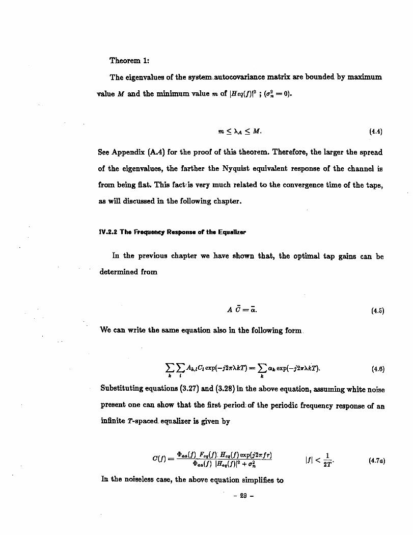
Theorem 1:

The eigenvalues of the system~~.autocOYaFiance matFix are bounded by maximum

value M and the minimum value m of l ~ e ~ ( f ) l ~ ; (a: = 0).

See Appendix (A.4) for the proof of this theorem. Therefore, the larger the spread

of the eigenvalues, the farther the Nyquist equivalent response of the channel is

from being flat. This fact:is very much related to the convergence time of the taps,

as will discussed in the following chapter.

IV.2.2 The Frequency Response of the Equalizer

In the previous chapter we have shown that, the optimal tap gains can be

determined from

We can write the same equation also in the following form

Substituting equations (3.27) and (3.28) in the above equation, assuming white noise

present one can show that the first period:;of the periodic frequency. response of an

infinite T-spaced. equalizer is given by

In the noiseless case, the above equation simplifies to

- 29 -

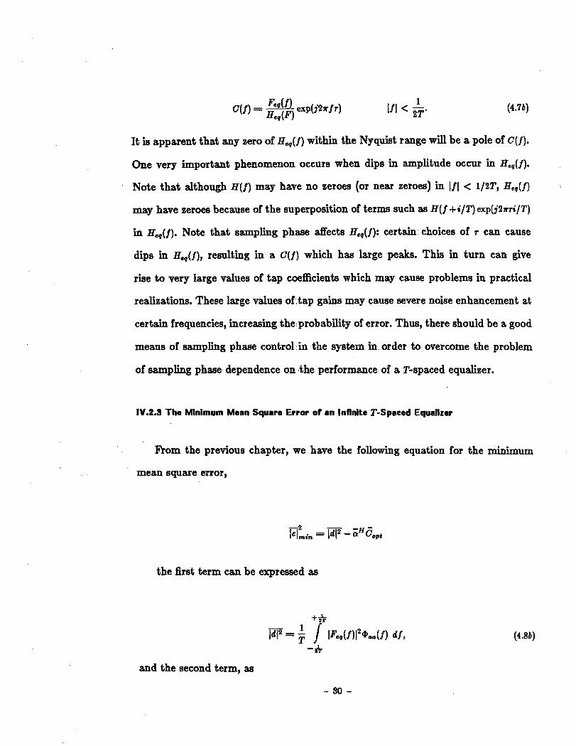
It is apparent that any zero of H,,(j) within the Nyquist range will be a pole of c(f).

One very important phenomenon occurs when dips in amplitude occur in H,,(j).

Note that although H(f) may have no zeroes (or near zeroes) in If 1 < l/2T, H,,(f)

may have zeroes because of the superposition of terms such as H(f +i/T) exp(j2nrilT)

in ~ , , ( f ) . Note that sampling phase affects H,,(f): certain choices of r can cause

dips in &,(I), resulting in a C(f) which has large peaks. This in turn can give

rise to very large values of tap coefficients which may cause problems in practical

reahations. These large values of tap gains may cause severe noise enhancement at

certain frequencies, increasing the probabiliQ of error. Thus, there should be a good

means of sampling phase control in the system in. order to overcome the problem

of sampling phase dependence on ,the performance of a T-spaced equalizer.

IV.2.3 The Mtnimum Mean Square Error of an Inflnite T-Spaced Equalizer

From the previous chapter, we have the following equation for the minimum

mean square error,

the first term can be expressed as

and the second term, as

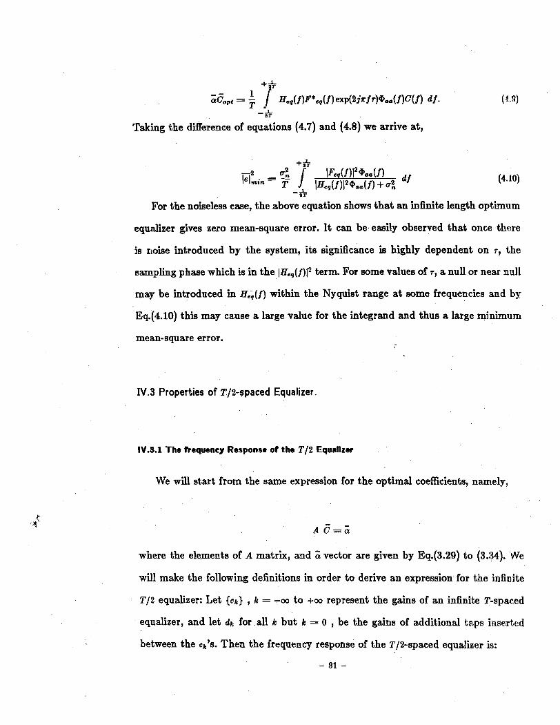
-2 I.,",;,, = $ I' e q 2 f d f

IHe,(f ) I 2 + . . ( f ) + 4 -_L ST

For the noiseless case, the above equation shows that an infinite length optimum

equalizer gives zero mean-square error. I t can be easily observed that once there

is noise introduced by the system, its significance is highly dependent on r, the

sampling phase which is in the I He,( f )J2 term. For some values of r , a null or near null

may be introduced in H 4 ( f ) within the Nyquist range a t some frequencies and by

Eq.(4.10) this may cause a large value for the integrand and thus a large minimum

mean-square error.

IV.3 Properties of ~/2-spaced Equalizer.

IV.3.1 The fkequeney Response o f the T / 2 EqualIra

We will start from the same expression for the optimal coefficients, namely,

where the elements of A matrix, and a vector are given by Eq.(3.29) to (3.34). We

will make the following definitions in order to derive an expression for the infinite

T/2 equalizer: Let { c k ) , k = -00 to +oo represent the gains of an infinite T-spaced

equalizer, and let dk for all k but k = 0 , be the gains of additional taps inserted

between the ck9s. Then the frequency response of the T/2-spaced equalizer is:

- 31 -

where:

and:

By using the same steps as in the. previous analysis for the T-spaced case, we come

up with (for & = H, ) :

C(f) = 2Feq(f) @ 4 f ) H*(f)ex~(j2nfr) (4.12)

@ d f ) l lkAfll2 + lH,(f12 1 + 4- The bracketed term in the denominator is equal to the folded power spectrum of

the overall response only when H(f) is bandlimited to If 1 < 1/2T, then we may write,

The above equation can be viewed as in two parts, the first being the matched

filter, and the other which combats the intersymbol interference. The matched filter

is matched to the averall.frequency response of the system up to the equalizer, for

the maximization of signal-to-noise ratio at the sampling instants.

A comparison of the C(f)'s for the T/t case and the conventional case indicates

that, there can be no poles caused by the denominator of C(f) within the Nyquist

range by the sampler timing offset r . In fact, the denominator of C(f) does not

depend on r and can be expressed in terms of the folded power spectrum of the

unequalized channel for systems bandlimited to 1/T.

IV.3.2 The Autoeorsrlanee Matrlx and its Efgenvalues

Just as in the conventional case one can show that the eigenvectors and the

eigenvalues of an infinite T/kspaced equalizer are given by [Qureshi and Forney,

19771:

and the corresponding eigenvalues, when (+) holds;

vn = I H . . ( ~ ~ + +l$.(n2,

and when (-) holds;

For H(f) bandlimited to I fl < 1/2T, X ( j ) can be expressed as the folded power

spectrum, i.e.

We see that a constant folded power spectrum in the T/2 case has the same effect as

a constant folded spectrum in the conventional case: in both cases it ie possible, by

a judicious choice of the step size to have the taps gains reach their optimal values

in one iteration.

Here, once again we observe that the eigenvalues are not dependent on the

sampling timing offset, r , whereas in the T-spaced equalizer the eigenvalue spread is

subject to change with r. Therefore we should expect the convergence of the infinite

length fractionally-spaced equalizer to be independent of sampler offset.

IV.3.3 The Minimum Mean Square Errw of an lnflnke T/2-Spaced Equalizer

In this section we will derive an expression for the minimum mean-square error

for a T/2 equalizer. By applying the similar procedure for the T equalizer case, the

mean-square error is given by:

- - - lelLin = ~ B U i3-aHd - = V i * V j w*uj - a i 4 opt - a k d k o p t J

i j even k odd k

can be expressed as:

It is seen here that mean-square error is not influenced by the sampling offset,

T . A comparison of the mean-square error expressions of the equalizers shows that,

i.e. the T i 2 equalizer performs better than the conventional case. It is also indepen-

dent of r. The simulation results in this thesis, aa well as in [Qureshi and Forney,

19771, [Ungerboeck, 19721 and [Ungerboeck, 19761 show these results clearly.

- 94 -

IV.4 Properties of HTE.

A hybrid type of equalizer was first introduced in [Nattiv and Kabal, 1980].

In their work they have defined the Hybrid Type EQualizer (HTE) as a T-spaced

equalizer with some additional intermediate taps inserted around the reference tap.

As these inserted taps had T/2 spacing with the adjacent taps, it is expected to have

many of the benefits of a T/2 equalizer, and have a wider time span compared to a

conventional equalizer with the same number of taps. This will enable the equalizer

to eliminate the intersymbol interference due to the channels with long impulse

responses. As additional taps are introduced to the T-spaced equalizer, the hybrid

equalizer will resemble that of a pure TJ2-equalizer. With the proper placement of

taps it is also expected that the hybrid type equalizer will avoid nulls, or near nulls

in the Nyquist range.

It will be shown in a later chapter that, the number of taps are related to the

final mean-square error. In other words, minimum achievable mean-square error

in steady-state is dependent on the number of taps, i.e. for larger N , beyond a

certain value, the mean-square error will be slightly larger due to the adaptation

fluctuations introduced by each tap. A hybrid equalizer reduces the complexity, as

well as using less number of taps the excess mean-square error term is minimized. It

is expected that the hybrid equalizer will be advantageous for both of these reasons.

In the following sections a summary of the work carried out by Nattiv [Nattiv,

and Kabal, 19801 will be presented. '

IV.4.1 The Optimal HTE

In the approach used to study the hybrid type equalizer, Nattiv considered the

overall system to be made up of a T-spaced, and a T/t-spaced part. In other words

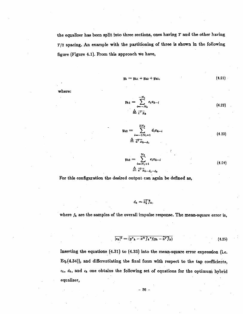
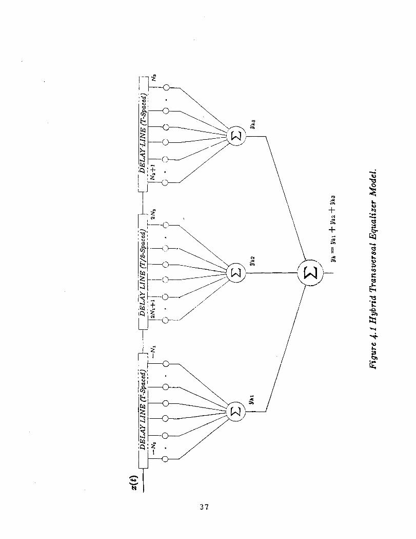
the equalizer has been split into three sections, ones having T and the other having

T / 2 spacing. An example with the partitioning of three is shawn in the following

figure (Figure 4.1). From this approach we have,

where: - NI

f lkl = cizk-i

For this configuration the desired output can again be defhed as,

where fk are the samples of the overall impulse response. The mean-square error is,

lek12 = ( Y * ~ - iHTk*)(yk - iTjk) (4.25)

Inserting the equations (4.31) to (4.33) into the mean-square error expression (i.e.

Eq.(4.34)), and differentiating the final form with respect to the tap coefficients,

ck, dk, and ek one obtains the following set of equations for the optimum hybrid

equalizer,

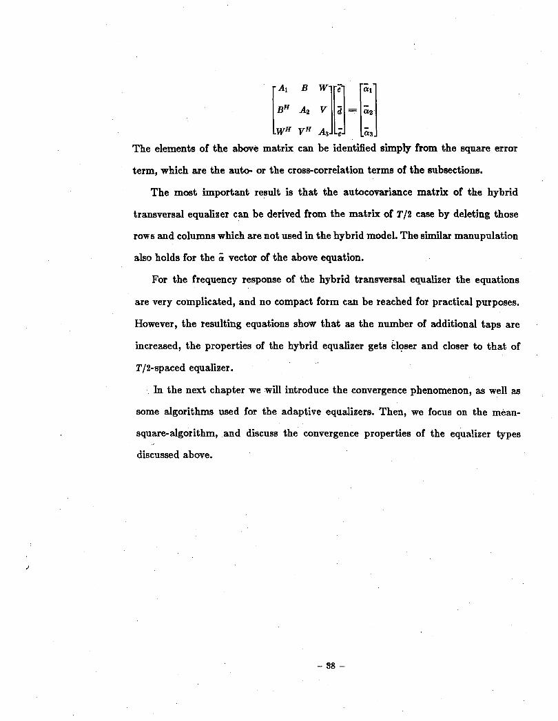
The elements of the above matrix can be identilied simply from the square error

term, which are the sub or the cross-correlation terms of the subsections.

The most important result is that the autocovariance matrix of the hybrid

transversal equalizer can be derived from the matrix of T / 2 case by deleting those

rows and columns which are not used in the hybrid model. The similar manupulation

also holds for the Z vector of the above equation.

For the frequency response of the hybrid transversal equalizer the equations

are very complicated, and no compact form can be reached for practical purposes.

However, the resulting equations show that as the number of additional taps are

increased, the properties of the hybrid equalizer gets closer and closer to that of

T/2-spaced equalizer.

In the next chapter we will introduce the convergence phenomenon, as well as

some algorithms used for the adaptive equalizers. Then, we focus on the mean-

square-algorithm, and discuss the convergence properties of the equalizer types

discussed above.

CHAPTER V

CONVERGENCE PROPERTIES of the TRANSVERSAL EQUALIZERS

V . l The Recursive Algorithms for Computing the Tap Gains

In this chapter we will introduce some of the techniques by which the tap

coefficients are adjusted, and then analyse the steepest descent algorithm. In the

rest of the chapter we will analyse the rate of convergence of the conventional

equalizer and discuss for the fractionally spaced and hybrid equalizer cases.

The adaptation of the transversal filter to the channel response and the source

signal is realized a t the receiver by an iterative procedure to adjust the tap weights.

The general adaptation method can be modelled by:

where the .?k is a vector of tap gain increments. There are various algorithms that

achieve adaptation. Many transversal filter equalizer update algorithms are based

- 39 -

on the steepest descent, or gradient technique, which minimizes the mean-square

error between the equalizer output and the transmitted data symbols, given by

One algorithm invokes the minimization of least square the objective of which is

to determine the coefficient vector which minimizes the weighted sum of the squared

errors of past received signal vectors [Mueller, 19811, in other words it minimizes

Setting the derivative of the above equation to equal to zero yields the discrete time

Wiener-Hopf equation,

in the iterative form,

and

A positive definite identity matrix A1 is included to ensure positive definiteness of

A = n for all n.

Since'the above two equations can be written recursively, the updated coefficient

can be found iteratively as follows,

- 40 -

- - -0

Cn = Cn-I+ 9n en

where g, is the Kalman gain defined w

This form leads to the Kalman, the fast Kalman, and the adaptive lattice algorithms

where in all cases the same cost function is minimized. The difference is in the

manner and the complexity with which it is achieved. [Mueller, 19811

In their work O.S. Kosovych and R.L. Pickholtz [9] proposed a new algorithm

to improve the convergence rate, namely overrelaxation iterative technique. Where

their method determines the coefficient value for all i, a t the (k + l)et iteration

acording to

. - - - w

C i (k+l) = C i (k) - :[ aij C j (k+l) aijcj (k) - 9i]

where w is the relaxation factor. In matrix form we have,

where E and D are the diagonal and strictly lower triangular matrices. Here the

inverse of the A matrix is never computed if the above equation is used (5.9). All of

the coefficients are updated prior to the reception of the next training pulse. This

is a departure from gradient techniques since they use only the previous values.

As another example, the works carried out by T.J. Schonfeld and M. Schwartz,

minimized the mean-square error by using variable step sizes after a specified

number of iterations. The so called First-Order and Second-Order algorithms use a

optimally determined step size in order to achieve minimum mean-square error.

- 41 -

These and other papers on the various algorithm on the convergence of adaptive

equalizers can be found in the references [16] to [22]. In the following section the

steepest descent algorithm will be studied using a constant step size parameter.

V.2 The Steepest Descent Algorithm

This section concentrate on the steepest descent technique to solve Equation

(3.15) iteratively to find the optimal tap values. The convergence and the stability

of the method will be discussed.

W.0.1 Performance Surface

The adjustment algorithm attempts to find the minimum of the mean-square

error as a function of the tap weights. First, one begins by choosing an initial

set of values for the set {c,) of tap gains. The gradient vector is measured, and

the next guess is obtained from the present state of weights by making a change

in the tap vector in the direction of the negative of the gradient vector (in the

opposite direction of the gradient vector). If the mean error square is reduced with

each change in the weight vector, the process will converge to a stationary point

regardless of the initial choice.

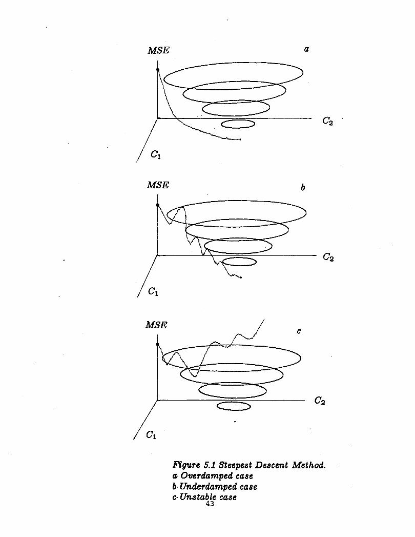
In Figure 5.la view of a two-dimensional (two tap) quadratic performance

surface is shown. The mean-square error is shown as along the z-axis and the

other coordinates are the two tap coefficients. The ellipses in the figures correspond

contours of constant mean-square error, spaced at equal increments. The gradient

must be orthogonal to these contours everywhere on the surface. In the following

figure ( Figure 5.la ) the series of small steps of the tap coefficients incremented

- 42 -

MSE a

MSE b

MSE I

Rgure 5.1 Steepest Descent Method. a- Overdamped case b- Underdamped case c- Unstable case

4 3

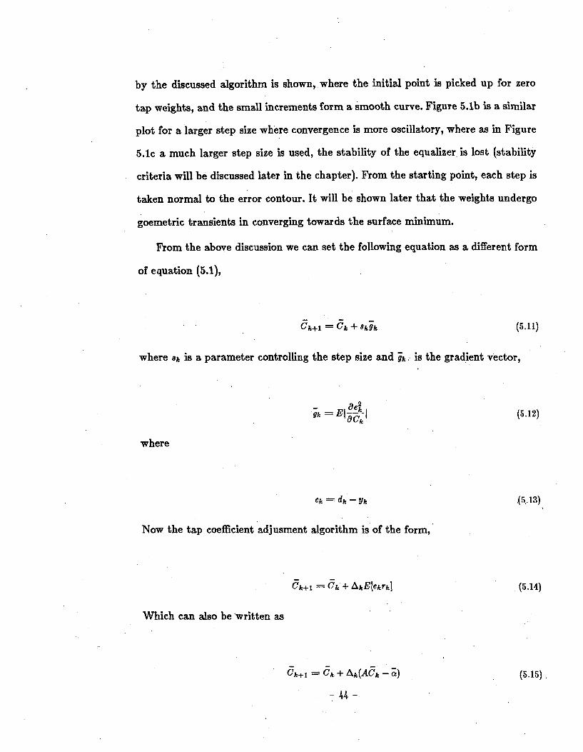
by the discussed algorithm is shown, where the initial point is picked up for zero

tap weights, and the small increments form a smooth curve. Figure 5.lb is a similar

plot for a larger step size where convergence is more oscillatory, where as in Figure

5.lc a much larger step size is used, the stability of the equalizer is lost (stability

criteria will be discussed later in the chapter). From the starting point, each step is

taken normal to the error contour. It will be shown later that the weights undergo

goemetric transients in converging towards the surface minimum.

From the above discussion we can set the following equation as a different form

of equation (5.1),

where 8k is a parameter controlling the step size and i k ; is the gradient vector,

where

ek = dk - Y k

Now the tap coefficient adjusment algorithm is of the form,

Which can also be 'written as

where Ak is the step size parameter (equal to 2ak), A is the correlation matrix of

the input sequence (on the assumption of t k and dk are stationary sequences). The

solution is

The conditions for convergence of the taps can be derived easily after the following

coordinate transformation.

V.2.2 Coordinate Transformation

In order to decouple the tap coefficient adjusments we will define the transfor-

mation,

where P is an orthonormal matrix which diagonalizes A. This transformation is

equivalent to a rotation of the coordinate system,

A = P-'A P (5.18)

and A is the diagonal matrix ofthe eigenvalues of xi of A . Then,

In Figure 5.2 a feedback model for this adjusment algorithm is shown. The optimum

decoupled weight vector can be written as,

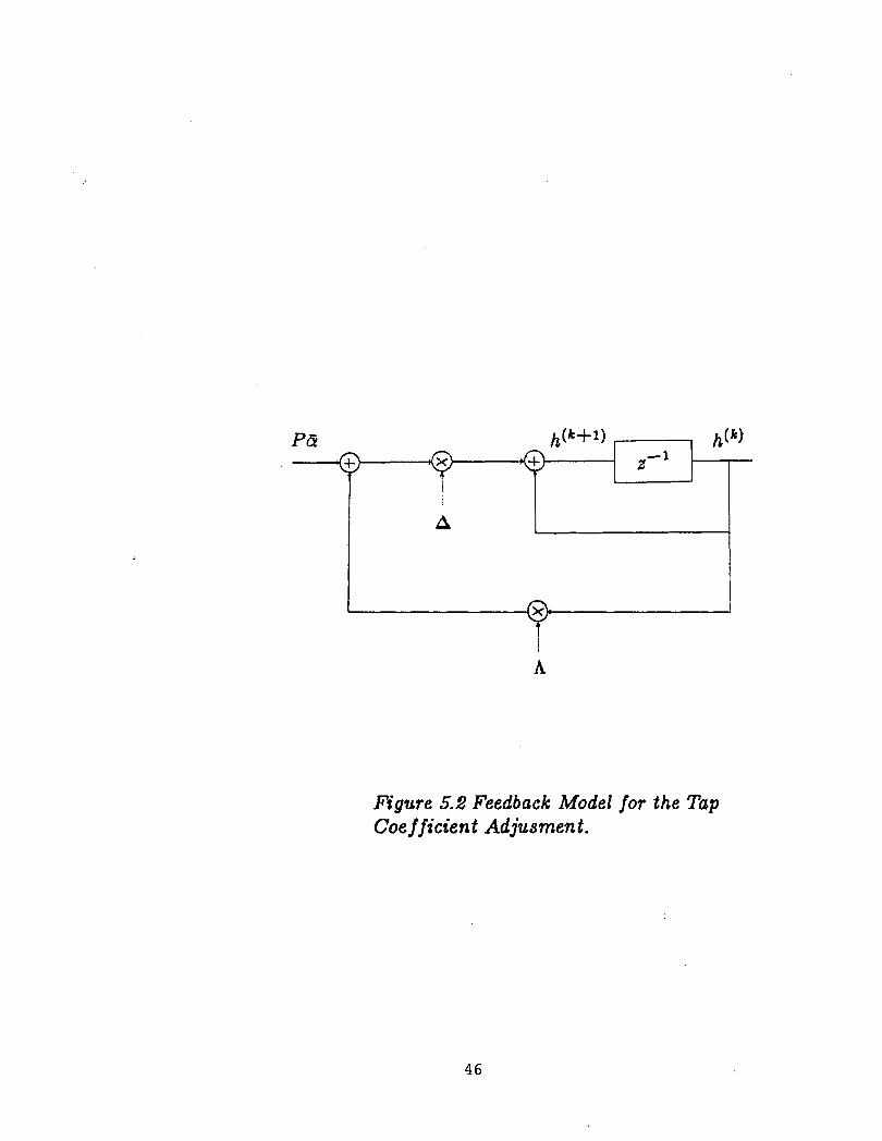
Figure 5.2 Feedback Model for the Tap Coe f w e n t Adjusment.

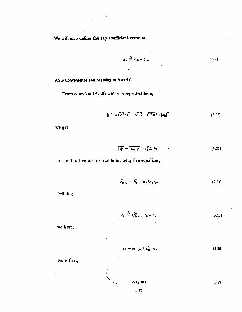
We will also define the tap coefficient error as,

V.2.3 convergence and Stability of h and C

From equation (A.I.3) which is repeated here,

we get

In the iterative form suitable for adaptive equalizer,

Defining

we have,

Note that,

which leads to

We will also restrict ourselves to a constant step size i.e. A~ = A. This gives us for

each j, j = 1, ...., M, the z-transform of the j'th tap weighting error as

Thle limit aa k -too of I ~ ~ ( k ) l is zero if and only if all of the poles of Hj(z) are within

the unit circle in the complex z-plane.

If

then,

The criteria for the convergence and the stability can be derived as follows. For

the positive definite autocovariance matrix A, we have i i T ~ E > 0, for all ;i. Then

from Eq.(5.15) by subtracting Copt from both sides

Makiig use of the coordinate transformation and the definition in Eq.(5.21),

For each of the decoupled components

- 48 -

hi(kt-1) = (1 - Ahi)hi(b) i = 1, ..., N

where hi is the ith eigenvalue of A. For convergence,

hi(k+l) < 11 - AXilhi(k)

for all k and i, which leads us to choose the step size acording to

Considering the maximum and the minimum values of the eigenvalues, and choosing

a step size of,

we get,

11 - Ah,&\ = ' A ~ ~ ~ - A&<n < 1 (5.38) 'Amam + 'Amin

Therefore a step size in the proper range will lead to convergence of the mean tap

values in the limit. Convergence in the mean does not depend on the number of

taps. If the mean square convergence is considered, stability does depend on the

number of taps[Mazo]. The convergence rate and stabilty is directly related to the

choice of A. Relating this to the channel response, if the channel response is flat

(the spread of the eigenvalues of the A matrix is small) the convergence will be fast.

V.3 Excess Mean-Square Error ( e l )

The measurement of noise in the recursive algorithm discussed above has a

mean-square error value that is proportional to the step size parameter (A). The

noise in the tap updating procedure due to the use of estimates rather than the

true value of the gradient components causes random fluctuations in the tap gains

about their optimal values. This leads to an increase in the mean-square error at

the output of the receiver. Thus the steepest descent algorithm will converge to

e:, + e i , in the mean-square sense, where e b is the variance of the measurement

noise.

The increase of MSE above the minimum achievable mean-square error due to

the estimation noise has been named "excess mean-square error", [Widrow 19661.

Since the amplitude of the random fluctuations of the'tap gains increase with an

increase in the value of the step size, one has to be careful in choosing this parameter.

A large step size will give a rapid adaptation, yet result in a higher excess MSE.

At any instant, using the set of (c,)'s we can write,

Using the coordinate transformations introduced earlier we have,

Where An are the eigenvalues of A. The average of the increase in the MSE due to

random fluctuations of the tap gains about their optimum values is given by;

Complete derivation of the computation of excess MSE using the signal and

system parameters can be found in [Proakis and Miller, 19691. The excess mean-

square error is

e2, = A N emin(@, + @nn)

2 (5.42)

Note that excess MSE is directly proportional to the nuc:' plr of taps and the step

size. This result is collaborated in our simulation results presented in the next

chaq~ter.

CHAPTER VI

RESULTS

Thie chapter is devoted to simulation results. The comparison of the equalizers

on the basis of their convergence properties follows the description of the methodol-

ogy used. A study of the dependence of the step size and the number of equalizer

taps is included.

VI . l Description of the Simulation

The digital adaptive fractional-tap equalizer was simulated using a computer

program. The program takes in the fraction of the symbol spacing, T I N , the overaJl

system response (including the reference point), then the desired channel response

(expressed in terms of the impulse response) is entered. The following transmission

and equalizer characteristics are also entered: signal-tenoise ratio, size of input d-

phabet (only a binary alphabet is used for this particular study), number of taps, the

subscript of reference tap (the program enables the user to change the particular

hybrid tap configuration), and the proportionality constant used in incrementing

the tap coefficients. Note that in order to keep the excess mean-square error ap-

proximately constant for configurations with different numbers of taps the step size

is made to vary with number of taps. Also, the number of training and transmitting

- 52 -

symbols are specified.

With the above input values, the program computes the channel autocovariance

matrix A and finds its eigenvalues. The optimum tap coefficients are calculated by

solving the simultaneous equations of (3.16). The optimum MSE is found using the

calculated optimum tap values. The tap coefficients are initialized (normally all

zero or to the optimal values for checking purposes), the symbols and the noise

components are generated using random number generating routines using the

system time base to randomize the starting point. Every sample value is convolved

with the overall system response, summed up with the noise component and passed

through the equalizer. The output of the equalizer is decoded and the taps are

updated using the steepest descent method. All the relevant data, such as the

particular hybrid tap settings, eigenvalues, optimal tap values, and the errors at

the output are stored for further analysis. Also, the output MSE after every ten

iterations, the calculated MSE using the optimal tap coefficients, the convergence

of the reference tap values, were utilized for plotting the necessary graphs.

Another program was also set up in order to find the optimal tap placings for the

hybrid configuration, where all the possible hybrid configurations were generated,

the optimum MSE was calculated, and for each additional tap, the minimum and

maximum MSE's along with the particular tap configuration used were recorded.

The results were used in choosing the placement of the additional taps.

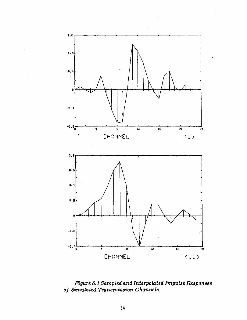
The results displayed in this thesis are the outputs of the simulations using the

two different channels which are selected from the papers [Ungerboeck],[Proakis].

In the rest of the chapter the channel responses will be referred as one (I) shown in

Figure 6.la, and the other (11) in Figure 6.lb. These channel responses have been

interpolated in order to obtain the intermediate samples.

CHANNEL ( 1 )

CHANNEL (11)

lifgure 6.1 Sampled and Interpolated Impulse Responees of Simulated Transmission Channels.

VI.2 Comparison of the Equalizers

In Figure 6.2, the relation between the minimum achievable MSE obtained by

directly solving (3.18) and the time span of the transversal equalizer is displayed for

a spaced equalizer. One should notice that the practical adaptive equalizers have

a higher MSE because of the excess mean-square error due to the noisy estimates in

the tap updating algorithm. This excess men-square error is a function of the step

size parameter and the number of taps. We shall discuss these two points later in

thik chapter. A similar plot was obtained for channel (11). These results show that

an equalizer time span of 10T ( 20 taps ) gives good results for both channels (I) and -

(II)

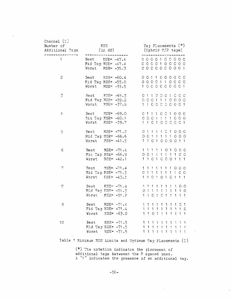
When different number of additional taps are inserted between the taps of the

T-spaced equalizer, it has been observed that the particular placement and the

number of additional taps play a considerable role in the minimum MSE. The best

and the worst MSE limits for every combination of the same number of additional

taps were calculated, and a plot is obtained for an equalizer spanning lor with

zero to ten additional taps. Although it seems that every additional tap reduces

the MSE, it should be apparent that the best placement of the additional taps is a

major concern. Since in most practical applications this information is not available,

a reasonable conjecture is that additional taps should be placed around the reference

tap. To test this, we have calculated the mean-square error when the additional taps

were clustered around the reference tap. In Figure 6.3, these results are plotted for

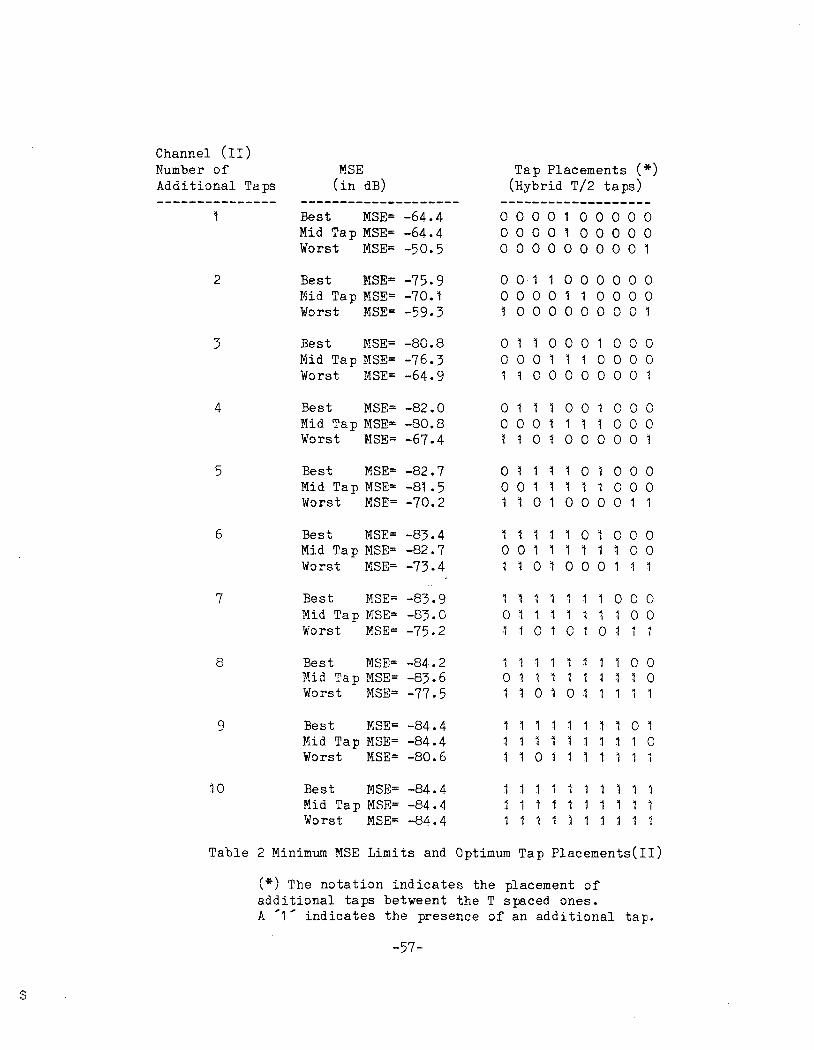
channels (I) and (11) respectively. The optimum and worst case tap placements are

given in Tables 1 and 2. It can easily be observed that the mid-taps are very good

approximations for the optimal hybrid equalizer configurations for both channels.

Therefore placing the additional taps around the reference tap seems to be a good

choice.

- 55 -

2 B e s t MSE= -63.4 C O 1 1 0 O O O O O K i d T a p MSE= -55.0 O O C O I 1 C O C O Worst MSE= -35.5 I G C O C C O C O 1

E e s t PIX=-65.3 C 1 1 O C O i C C G N i d Tay: MSE= -59.2 C C O 1 : ; 0 3 0 0 Worst MSE= -37.8 i 1 G O C 3 C C 0 1

Best YSE= -59.6 ., . ' C f 1 1 C 0 1 O C C !:lid T a p KSE= -60.1 C C C I I I 1 C C O Worst KSE= -39.7 l l C I C C C G O 1

S e s t WE=-7f.2 C 1 1 i 1 0 1 0 0 C Kid T a p ESE= -66.6 O C l f 1 1 1 G O O $Jars t 9 S E = -41.3 1 1 C 1 G O O C I 1

B e s t MSE= -71 .4 1 ; 1 1 1 01 O O C Ifid T a p IISE= -65.9 O C I : 1 1 I 1 C C V o r s t ?E2= -42.1 1 1 01 C C O I 1 1

Z e s t NSE= -71 .4 1 1 1 1 7 1 1 0 C C H i d Ts p KSE= -71 .: n L ~ l l l l ? I C C 4

X ~ r s t I?SE= -43.3 I 1 C 1 0 1 G I : 1

Bes t ItSE=-71.4 1 1 4 1 1 1 1 1 0 0 Mid T a p F S E = -71 .3 Q 1 1 I I ~ l I I ~ Worst KSE= -51 .2 1 1 0 1 C 1 1 1 1 1

E e s t YSE= -71 . 4 1 1 1 1 1 1 1 l C l ?<!id Tap KSE= -71 .4 1 1 1 1 1 1 1 1 1 C 'do rs t KSE= -63.5 1 1 @ 1 1 1 1 i 1 1

1 C E e s t MSE= -7: .5 1 1 1 1 1 1 1 1 1 1 F i d ? a ~ MSE= -71 .5 1 1 1 1 1 1 1 1 1 1 Worst r:'iSE= -71 .5 l l l l l l i l l l

T a b l e 1 Mininum YSE L i m i t s and Optimum T ~ F P l a c e m e n t s ( I )

(*) The n o t a t i o n i n d i c a t e s t h e p lacement o f a d d i t i o n a l t a p s be tween t t h e T spaced ones . k '1 ' i n d i c a t e s t h e p re sence o f an a d d i t i o n a l t a p .

Channel (11) Number o f MSE A d d i t i o n a l Taps ( i n d ~ )

2 Best MSE=-75.9 Mid Tap MSE= -70. ? Worst MSE= -59.3

Best NSE= -80.8 Mid Tap MSE= -76.3 Worst YSE= -64.9

Best MSE=-82.0 Mid Tap MSE= -80.8 W3rst MSE= -67.4

Best MSEr-82.7 Mid Tap MSEr -81 .5 Worst MSE= -70.2

Best PEE= -83.4 Mid Tap WE= -82.7 Worst KSEr -73.4

Tap Placements (*) ( ~ ~ b r i d ~ / 2 t a p s )

0 1 1 7 0 0 1 C O O 0 0 0 1 1 1 1 C O O 1 7 0 1 0 0 C 0 0 1

0 1 1 4 4 0 1 O O C 0 0 1 1 ? 1 1 0 0 0 1 3 0 1 0 0 0 0 1 1

9 3 7 1 ' 1 0 1 c c o 0 0 1 1 1 1 1 1 G O I 1 0 1 0 0 0 1 1 1

Best MSE= -83.9 1 1 1 5 1 1 1 C O O Mid Tap MSE= -63.0 0 1 1 1 1 1 1 1 0 0 Worst MSE= -75.2 1 1 G 1 G I 0 1 1 1

Bes t MSE= -84.2 1 1 1 1 1 1 1 1 0 0 M i d Tap MSE= -83.6 0 1 1 1 ~ 1 1 1 1 0 Worst MSE= -77.5 1 1 0 1 0 1 1 1 1 1

Best MSEP -84.4 1 1 1 1 1 1 1 1 0 1 Mid Tap MSE= -84.4 : 1 1 1 1 1 1 1 1 0 Worst MSE= -80.6 1 1 0 1 1 1 1 1 1 ;

10 Best MSE=-84.4 1 1 1 1 1 1 1 1 1 1 Mid Tap MSE= -84.4 1 1 1 1 1 1 1 t 1 1 Worst MSE= -84.4 1 1 1 1 1 1 1 1 1 1

T a b l e 2 Minimum MSE L i m i t s and Optimum Tap ~ l a c e m e n t s ( 1 1 )

(*) The n o t a t i o n i n d i c a t e s t h e placement o f a d d i t i o n a l t a p s betweent t h e T spaced ones. P. -1 @ i n d i c a t e s t h e presence o f an a d d i t i o n a l t a p .

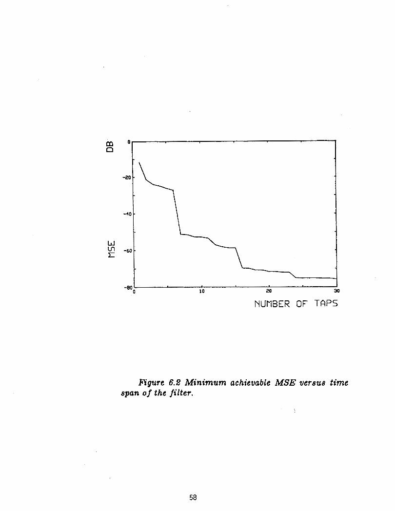
NUMBER OF TAPS

8Igut.e 6.2 Minimum achievable MSE versus time span of the filter.

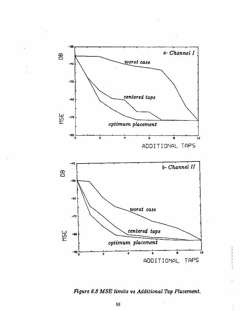
a- Channel I

optimum placement

6- Channel I1

optimum placement -

ADDITIONAL TAPS

Figure 6.8 MSE limits us Additional Tap Placement.

59

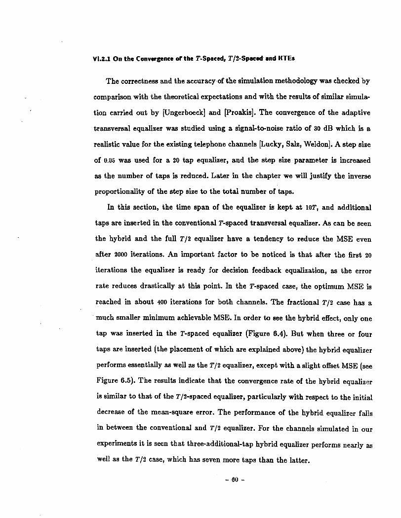
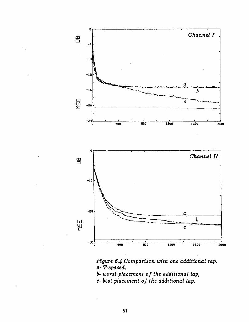
V1.2.1 O n the convergence of the T-Spaced, T/2-Spaced and HTEs

The correctness and the accuracy of the simulation methodology was checked by

comparison with the theoretical expectations and with the results of similar simule

tion carried out by [Ungerboeck] and [Proakis]. The convergence of the adaptive

transversal equalizer was studied using a signal-tenoise ratio of 30 dB which is a

realistic value for the existing telephone channels [Lucky, Salz, Weldon]. A step size

of 0.05 was used for a 20 tap equalizer, and the step size parameter is increased

as the number of taps is reduced. Later in the chapter we will justify the inverse

proportionality of the step size to the total number of taps.

In this section, the time span of the equalizer is kept at 10T, and additional

taps are inserted in the conventional T-spaced transversal equalizer. As can be seen

the hybrid and the full T/2 equalizer have a tendency to reduce the MSE even

after 2000 iterations. An important factor to be noticed is that after the first 20

iterations the equalizer is ready for decision feedback equalization, as the error

rate reduces drastically at this point. In the T-spaced case, the optimum MSE is

reached in about 400 iterations for both channels. The fractional T/2 case has a

much smaller minimum achievable MSE. In order to see the hybrid effect, only one

tap was inserted in the T-spaced equalizer (Figure 6.4). But when three or four

taps are inserted (the placement of which are explained above) the hybrid equalizer

performs essentially as well as the T/2 equalizer, except with a slight offset MSE (see

Figure 6.5). The results indicate that the convergence rate of the hybrid equalizer

is simiiar to that of the T/2-spaced equalizer, particularly with respect to the initial

decrease of the mean-square error. The performance of the hybrid equalizer falls

in between the conventional and T/2 equalizer. For the channels simulated in our

experiments it is seen that three-additional-tap hybrid equalizer performs nearly as

well as the T/2 case, which has seven more taps than the latter.

Channel II

Figure 6.4 Comparison with one additional tap. a- T-spaced, 6- worst placement of the additional tap, c- best placement o j the additional tap.

Figvre 6.5 Comparison o f the three cases. a- T Spaced Eqzsa lizer b- Hybrid Equalizer with three additional taps c- T/2 Spaced Equalizer

VI.3 The Excess-MSE(e2, ) and the Stability Limits

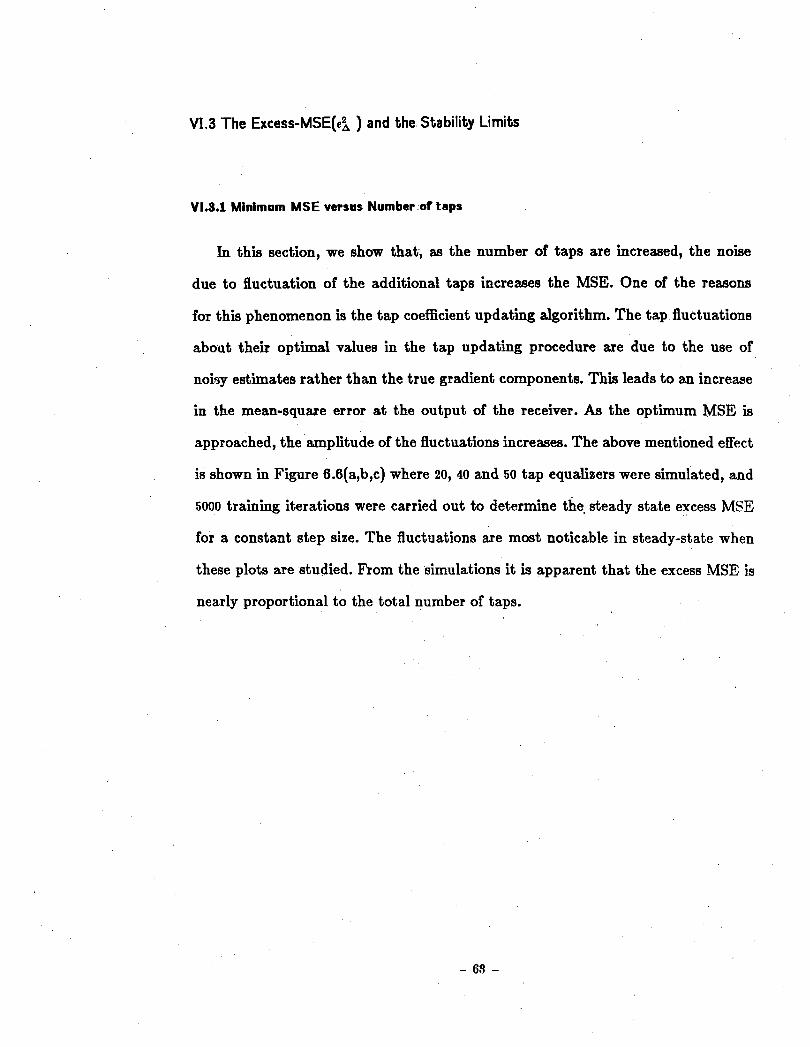
V1.3.1 Minimum MSE versus Number of taps

In this section, we show that, as the number of taps are increased, the noise

due to fluctuation of the additional taps increases the MSE. One of the reasons

for this phenomenon is the tap coefficient updating algorithm. The tap fluctuations

abaut their optimal values in the tap updating procedure are due to the use of

noit-y estimates rather than the true gradient components. This leads to an increase

in the mean-square error at the output of the receiver. As the optimum MSE is

approached, the amplitude of the fluctuations increases. The above mentioned effect

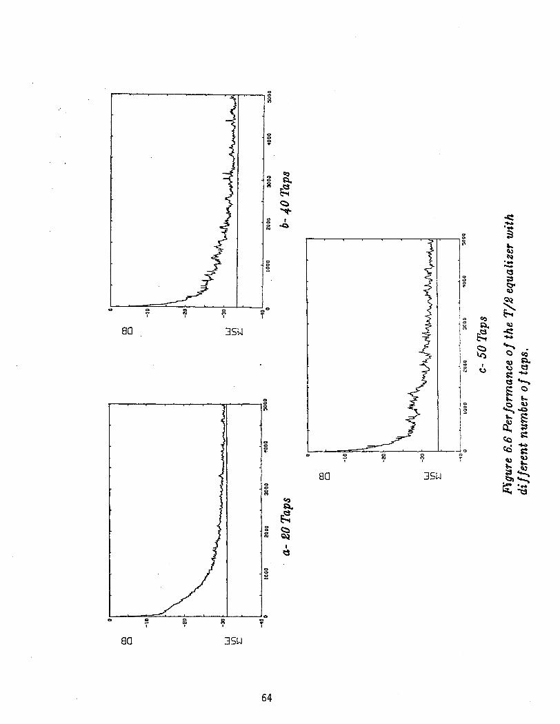
is shown in Figure 6.6(a,b,c) where 20, 40 and 50 tap equalizers were simulated, and

5000 training iterations were carried out to determine the steady state excess MSE

for a constant step size. The fluctuations are most noticable in steady-state when

these plots are studied. From the simulations it is apparent that the excess MSE is

nearly proportional to the total number of taps.

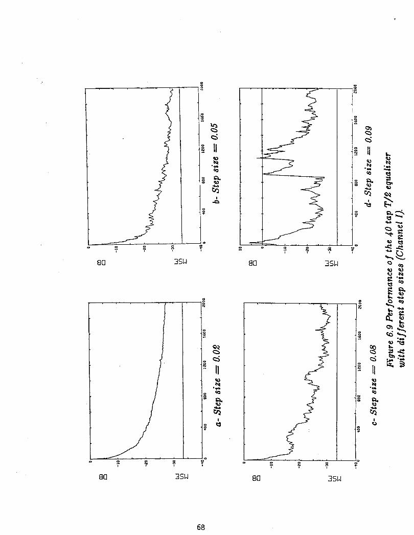
VI.S.2 E m e t s of Step Size on Excess-MSE and Stab-

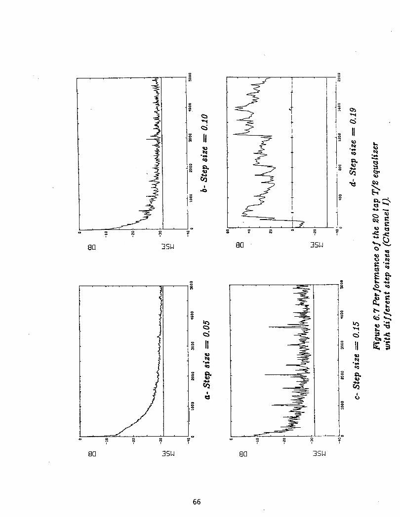
The step size is a major concern for the optimization of the system. Although, a

fast convergence is realized with a larger step size, the fluctuations (excess MSE) are

considerably more a t the later portion of the operation. If the step size is large (the

absolute size is determined by the number of taps and the channel noise level) it has

been observed that the equalizer is unstable, and that it diverges from the optimal

values after a few iterations (Figure 6.7). This represents a serious breakdown for

a decision-directed operation where the equalizer is in the receiving stage. In the

following figures only the step size of the equalizer has been changed. In the first part

of Figure 6.7 a step size of 0.05 has been used and resulted in a smooth convergence

and a steady minimum MSE. In the other two cases step sizes of 0.10 and 0.15 were

used. Although this results in a faster rolloff in the beginning, larger step size gives

rise to a higher steady-state mean-square error as well as the fluctuations about the

optimal tap values have large peaks compared to the step size of 0.05 case.

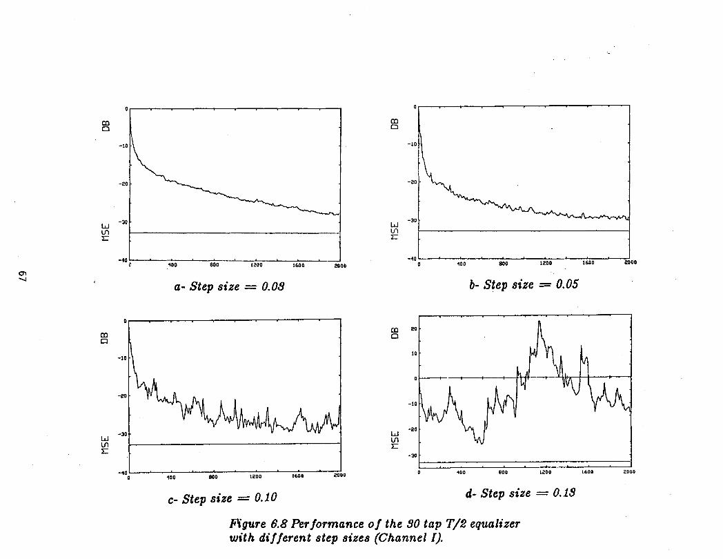
The same simulation is also carried out when the number of taps were chauged

from 20 to 30 to 40 in order to see the constraint on the step size for stability. As

seen in Figures 6.8 and 6.9, it can be observed that for different number of taps the

equalizers show the following results; (i) For a larger number of taps the step size has

to be smaller for a smooth performance, (ii) The equalizers with fewer number of

taps can use a much larger step size giving a more rapid hdaptation. The maximum

step size is determined by the total number of taps which is determined by the

stability limit.

The simulations carried out in this chapter have been done using the two

channels. The results for channel I1 have not been included a3 they show similar

trends. In the next chapter, we present a general summary of the thesis as well as

the conclusion derived from the theory, expectations and results.

a- Step size = 0.08

-40 1 0 100 800 1200 1600

c- Step size = 0.10

b- Step size = 0.05

d- Step size = 0.18

Figure 6.8 Performance o f the SO tap T/2 equalizer with different step sizes (Channel I).

SUMMARY and CONCLUSION

h this thesis we introduced a.generalized digital transmission system and then

studied the optimization of such a system. A receiver optimization strategy is chosen

because the channel characteristics and the behaviour of noise is in general unknown.

Thus we started analysing the receiver and came up with a suboptimal realizable

receiver. This involves a low-pass filter, a transversal filter and a decision unit.

Once the form of the system is known, the low-pass filter and the decision unit

are placed in the receiver. We have concentrated on the transversal filter section

of the receiver. The weighted sums of the past and future samples (relative to the

reference tap) of the signal are available at the output of the transversal filter.

The elimination of intersymbol interference can be handled once the tap weights

of the transversal filter are derived. Inorder to find these tap coefficients we have

selected to minimize the mean-square error. This led to a derivation of a generalized

equalizer model which has arbitrary tap positions. This analysis was used when the

particular equalizers were studied, the T-spaced, T/t-spaced and the hybrid cases.

We have tried to extract the properties of the above mentioned equalizers considering

their frequency responses, the autocovariance matrix and their eigenvalues, and the

mean-square error. For each case the equalizer is assumed to be infinite.

The algorithms that can be applied to find the tap coefficients iteratively were

introduced. The steepest descent method was discussed and used in the simulations.

The convergence, the stability constraints were also discussed. The dependence of

' - 6 9 -

the number of taps as well as the step size to the convergence behaviour of the

equalizer was shown. One of the variables namely the excess mean-square error was

derived to prove some results.

The simulation results showed the benefits and the limitations of the three

equalizers studied. It has been observed that the step size is an important factor in

stability and the convergence of the equalizers. When a small step size is used, the

convergence to the optimum tap settings is reached very slowly, and the fluctuations

arou.nd the minimum mean-square error is small. A larger step size gives rise to a

faster adaptation yet it has a considerable excess mean-square error at the steady

state. It is also apparent from the simulations that the number of taps has an

important role in the performance of the adaptation behaviour of the equalizers.

The step size and the number of taps are directly related in the performance.

When the number of taps is large, the excess mean-square error increases, and for

particular conbination of step size and number of taps, it is shown that the equalizer

is unstable. Which in turn shows the inverse proportionality between the step size

and the number of taps. The superiority of the hybrid type equalizer comes into

effect at this moment. Since the convergence rate depends on the step size, one can

obtain larger step sizes than T / 2 case since in has less number of taps for the same

timespan.

Therefore the final word we will state is that the hybrid equalizer has most of

the properties of the T/2 spaced equalizer in terms of convergence, and superior in

terms of stablity. Also having less number of taps reduces the excess mean-square

error as well as the complexity of the system. Although we have not studied the

effects of the sampling phase when a hybrid equalizer is used, the study by Nattiv

shows that it is much less dependent compared to the conventional equalizer.

LITERATURE

[I] G. Ungerboeck, Tractional Tap-Spacing Equalizers and Consequences

for Clock Recovery in Data Modems", IEEE Trans. on Comrn. ,vol.

Com-24, pp. 856-864, August 1976.

[2] G. Ungerboeck, 'Theory on the Speed of Convergence in Adaptive

Equalizers for Digital Communicationn, IBM J. Res. Develop. , vol.

V-16, pp. 546-555, November 1972..

[3] J. G. Proaki, "An Adaptive Receiver for Digital Signalling

Through Channels With Intersymbol Interferenceu, IEEE Trans. on

Information Theory, vol. IT-15, pp. 484497, July 1969.

[4] S. U. H. Qureshi and D. Forney, "Performance and Properties of T/2

Equalizer", NTC '77, pp. 11:l.l-11:1.9, 1977.

[5] R. D. Gitlii and S. B. Weinstein, 'Tractional Spaced Equalization: An

Improved Digital Transversal Equalizern, BSTJ,vol. 60, pp. 275-294,

1 February 1981.

[6] M. S. Mueller, "Least-Squares Algorithms for Adaptive Equalizers",

BSTJ,vol. 60, pp. 193-213, October 1981.

[7] B. Widrow, Adaptive Filters, in " Aspects of Network and System

Theory", Kalman R. E. and Declark N.(Eds.), Holt Rinehart and

Winston, pp. 563-587, 1971.

[8] H. Rudin, "Automatic Equalization Using Transversal Filters", IEEE

Spectrum, pp. 53-59, January 1967.

[9] 0. S. Kosovych and R. L. Pickholtz, 'Automatic Equalization Using

- 71 -

a Successive Overrelaxation Iterative Techniquen, IEEE Trans. on

Information Theory,vol. IT-21, pp. 51-58, January 1975.

[lo] R. W. Lucky, J. Salz and E. J. Weldon, " Principals of Data

Communicationn, New York, McGraw-Hill, 1968.

[ll] R. W. Lucky, "Automatic Equalization for Digital Communication.",

BSTJ, vol. 44, p. 547, 1965.

[I21 R. W. Lucky, "Techniques for Adaptive Equalization of Digital

Communication Systems.", BSTJ, vol. 45, p. 255, 1965.

[13] R. W. Lucky and H. R. Rudin, KAn Automatic Equalizer for General-

Purpose Communication Channels.", BSTJ, vol. 46, p. 2197, 1967.

[14] A. Gersho, "Adaptive Equalization for Highly Dispersive Channels for

Data Transmission", BSTJ, vol. 48, p. 55, 1969.

[I51 D. Hirsch and W. J. Wolf, "A Simple Adaptive Equalizer for Efficient

Data Transmission.", IEEE Trans. on Communication, vol. Com-18,5

[16] R. W. Chang, "A New Equalizer Structure for Fast Start-up Digital

Communication.", BSTJ, vol. 50, p. 143, 1971.

I171 T. J. Schonfeld and M. Schwartz, "A Rapidly Converging First-

Order Training Algorithm for an Adaptive Equalizer", B E E Trans.

on Information Theory, vol. IT-21, pp. 431-439, July 197 1.

[IS] J. E. Mazo, "On the Independence Theory of the Equalizer

Convergence", BSTJ, vol. 58, pp. 963-983, May-June 1979.

[19] T. Ericson, "Structure of Optimum Receiving Filters in Data

' - 7 2 -

Transmission Systems", IEEE Tran. on Information Theory, vol. IT-

17, pp. 352353, May 1971.

M. S. Mueller, "On the Rapid Initial Convergence of Least-Squares

Adjustment Algorithmsn, BSTJ, vol. 60, pp. 2345-2359, December

1981.

T. J. Schonfeld and M. Schwartz, " Rapidly Converging Second-Order

Tracking Algorithms for Adaptive Equalizationn, IEEE Trans. on

Information Theory, vol. IT-17, pp. 572-579, September 1971.

M. Nattiv, "Fractional Tap-Spacing Equalizers for Data

Transmission", M. Eng. Thesis, M c G i University, Electrical

Engineering Dept. , 1980.

APPENDIX

A.l The Derivation of Equation (3.16)

We start from the mean of the square error, as in equation (3.15)

Making use of the vector notations defined in the related sections, one obtains

= @HZ* - dk*) ( 2 ~ 8 - - d ) .

By defining the following matrix and vector

- A - a = Zk dk*,

the result of the above mean-square error term is of the following form

All of the vectors in the above equation are complex, i.e. C = ~ e { f ? ) + j lm{C) . To

minimize the mean-square error $ term with respect to , we have to differentiate

it with respect to Re[ck] and j I m [ c k ] for every k . We define complex functions that,

* \.IH is the conjugate-transpose operation.

- 74 -

= ~ A C - 2;.

Setting the derivative to zero,

- 2ACOpt - 2a = 0

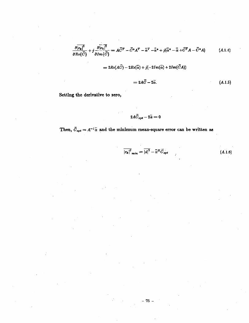
Then, Copt = A-'a and the minimum mean-square error can be written as

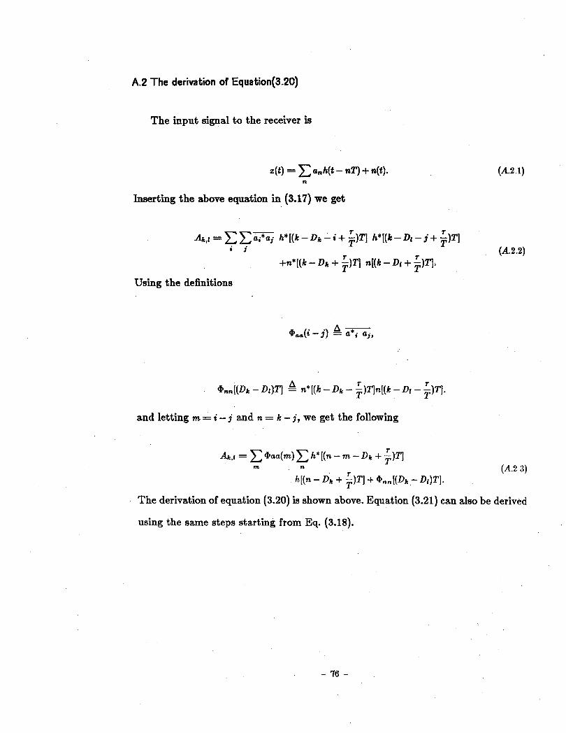
A.2 The derivation of Equation(3.20)

The input signal to the receiver is

Inserting the above equation in (3.17) we get

r r lq,r=xxai'.,. h e [ ( ) - D k - i + ? ; ) q h e [ ( ) - D l - j + ? ; ) q i j (A.2.2)

r r +n*[(k - D i + ?)TI n[(k -Dl + $TI.

Using the definitions

A r r ann[(Dr - D [ ) 4 = n*[(k - Dk - - ) q n [ ( k -Dl - ?;)TI. T

and letting m = i - j and n = k - j, we get the following

r Ak,l = C aaa(m) C h*[(n - m - Dk + --)TI

m n T

r (A.2 3) h [ (n - Dk + ?;)TI + @nn[(Dk - D I ) T ] -

The derivation of equation (3.20) is shown above. Equation (3.21) can also be derived

using the same steps starting from Eq. (3.18).

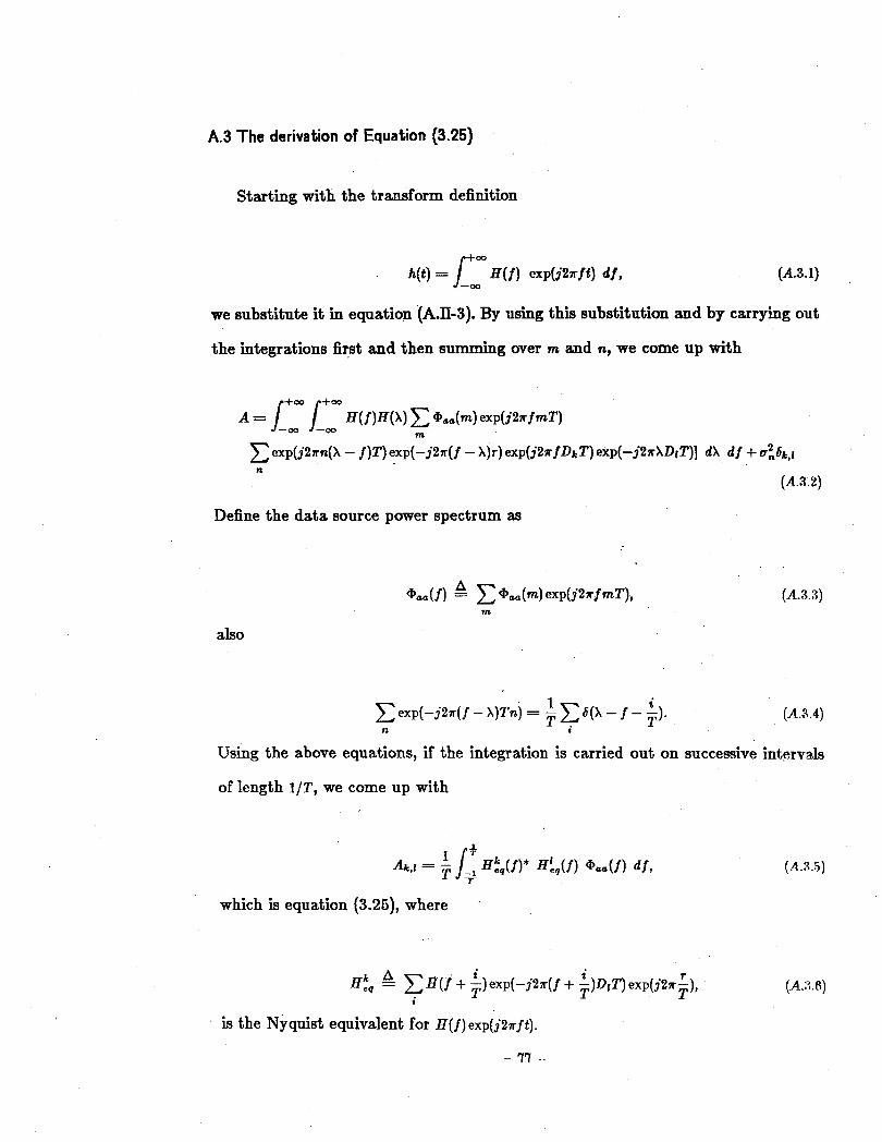
A.3 The derivation of Equation (3.25)

Starting with the transform definition

we substitute i t in equation (A.II-3). By using this substitution and by carrying out

the integrations first and then summing aver m and n, we come up with

Define the data source power spectrum as

also

Using the above equations, if the integration is carried out on successive intervals

of length 1/T, we come up with

which is equation (3.25), where

k h i i H., - C H ( j + + e x p ( - j 2 r ( j + -)D~T) e x p ( j 2 r L ) , T T t

is the Nyquist equivalent for ~ ( f ) e x p ( j 2 n j t ) .

- 77 -

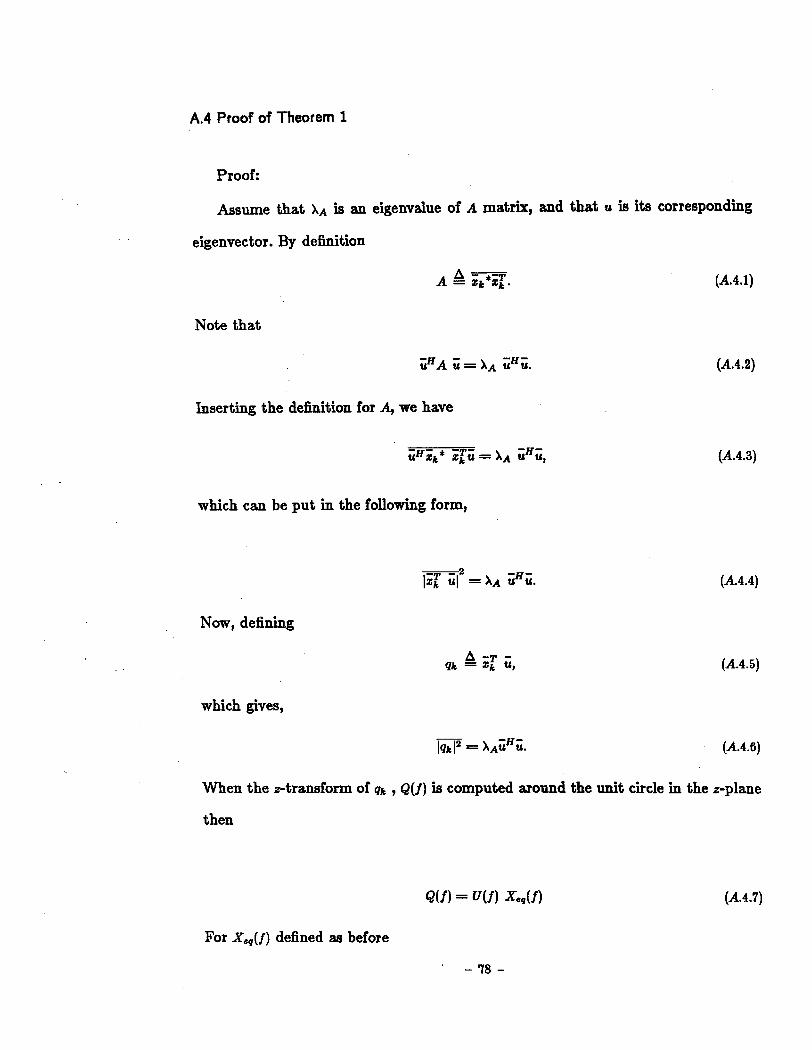
A.4 Proof of Theorem 1

Proof:

Assume that X A is an eigenvalue of A matrix, and that u is its corresponding

eigenvector. By definition

A - A = X ~ * % . (A.4.1)

Note that

Inserting the definition for A, we have

-H- ;HZk* E:; = X A u U,

which can be put in the following form,

Now, defining

which gives,

When the Z-transform of q k , &(I) is computed around the unit circle in the z-plane

then

For X,,(f) defined as before

' - 7 8 -

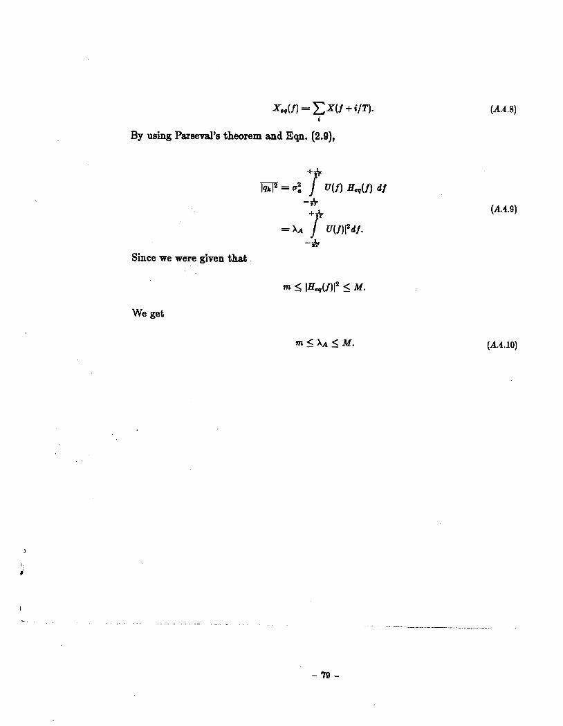
By using Parsed's theorem and Eqn. (2.9),

-* = X A 7 U(f)I2df .

-1 ST

Since we were given that

We get