
Control of a mechanical hybrid powertrain - TU/e · Control of a mechanical hybrid powertrain...
264
Control of a mechanical hybrid powertrain Citation for published version (APA): Berkel, van, K. (2013). Control of a mechanical hybrid powertrain. Eindhoven: Technische Universiteit Eindhoven. https://doi.org/10.6100/IR755483 DOI: 10.6100/IR755483 Document status and date: Published: 01/01/2013 Document Version: Publisher’s PDF, also known as Version of Record (includes final page, issue and volume numbers) Please check the document version of this publication: • A submitted manuscript is the version of the article upon submission and before peer-review. There can be important differences between the submitted version and the official published version of record. People interested in the research are advised to contact the author for the final version of the publication, or visit the DOI to the publisher's website. • The final author version and the galley proof are versions of the publication after peer review. • The final published version features the final layout of the paper including the volume, issue and page numbers. Link to publication General rights Copyright and moral rights for the publications made accessible in the public portal are retained by the authors and/or other copyright owners and it is a condition of accessing publications that users recognise and abide by the legal requirements associated with these rights. • Users may download and print one copy of any publication from the public portal for the purpose of private study or research. • You may not further distribute the material or use it for any profit-making activity or commercial gain • You may freely distribute the URL identifying the publication in the public portal. If the publication is distributed under the terms of Article 25fa of the Dutch Copyright Act, indicated by the “Taverne” license above, please follow below link for the End User Agreement: www.tue.nl/taverne Take down policy If you believe that this document breaches copyright please contact us at: [email protected] providing details and we will investigate your claim. Download date: 06. Apr. 2020
Transcript of Control of a mechanical hybrid powertrain - TU/e · Control of a mechanical hybrid powertrain...

Control of a mechanical hybrid powertrain
Citation for published version (APA):Berkel, van, K. (2013). Control of a mechanical hybrid powertrain. Eindhoven: Technische UniversiteitEindhoven. https://doi.org/10.6100/IR755483
DOI:10.6100/IR755483
Document status and date:Published: 01/01/2013
Document Version:Publisher’s PDF, also known as Version of Record (includes final page, issue and volume numbers)
Please check the document version of this publication:
• A submitted manuscript is the version of the article upon submission and before peer-review. There can beimportant differences between the submitted version and the official published version of record. Peopleinterested in the research are advised to contact the author for the final version of the publication, or visit theDOI to the publisher's website.• The final author version and the galley proof are versions of the publication after peer review.• The final published version features the final layout of the paper including the volume, issue and pagenumbers.Link to publication
General rightsCopyright and moral rights for the publications made accessible in the public portal are retained by the authors and/or other copyright ownersand it is a condition of accessing publications that users recognise and abide by the legal requirements associated with these rights.
• Users may download and print one copy of any publication from the public portal for the purpose of private study or research. • You may not further distribute the material or use it for any profit-making activity or commercial gain • You may freely distribute the URL identifying the publication in the public portal.
If the publication is distributed under the terms of Article 25fa of the Dutch Copyright Act, indicated by the “Taverne” license above, pleasefollow below link for the End User Agreement:www.tue.nl/taverne
Take down policyIf you believe that this document breaches copyright please contact us at:[email protected] details and we will investigate your claim.
Download date: 06. Apr. 2020

Control of a mechanical hybrid powertrain
koos van berkel
Koos van Berk
el
Control of a mechanical hybrid pow
ertrain
Invitation
You are cordially invited to the public defense of my PhD thesis:
Control of a mechanical hybrid powertrain.
You are also welcome to the reception afterwards.
Koos van Berkel
Date:Wednesday July 3rd 2013
Time: 16:00
Location:Auditorium 4 Eindhoven Universityof Technology
Contact:[email protected]

Control of a mechanical hybrid powertrain
Koos van Berkel

The research leading to this dissertation has received financial support from the“Pieken in de Delta” program, which is funded by the Dutch Ministry of EconomicAffairs, Province Noord-Brabant, and Samenwerkingsverband Regio Eindhoven.
The research leading to this dissertation is part of the “mecHybrid” project, which isa research project initiated by Drivetrain Innovations B.V., in consortium withEindhoven University of Technology, Punch Powertrain, Bosch TransmissionTechnologies, Centre Concepts Mechatronics B.V. (CCM), and SvenskaKullagerfabriken (SKF).
The research leading to this dissertation is part of the research program of the DutchInstitute of Systems and Control (DISC). The author has successfully completed theeducational program of the Graduate School DISC.
A catalogue record is available from the Eindhoven University of Technology LibraryISBN: 978-90-386-3406-7NUR: 978
Cover art by Geert van Leeuwen, geertvanleeuwen.com.Cover design by Veerle van Werde, veerleontwerpt.nl.Reproduction by Ipskamp Drukkers B.V., Enschede, the Netherlands.
c©2013 by Koos van Berkel. All rights reserved.

Control of a mechanical hybrid powertrain
PROEFSCHRIFT
ter verkrijging van de graad van doctor aan deTechnische Universiteit Eindhoven, op gezag van de
rector magnificus, prof.dr.ir. C.J. van Duijn, voor eencommissie aangewezen door het College voor
Promoties in het openbaar te verdedigenop woensdag 3 juli 2013 om 16.00 uur
door
Koos van Berkel
geboren te Heeze

Dit proefschrift is goedgekeurd door de promotor:
prof.dr.ir. M. Steinbuch
Copromotor:dr.ir. T. Hofman


Samenstelling promotiecommissie:
prof.dr. L.P.H. de Goey (voorzitter)prof.dr.ir. M. Steinbuch (promotor)dr.ir. T. Hofman (co-promotor)prof.dr. I. Kolmanovsky, University of Michigan (lid kerncommissie)dr.habil. S. Delprat, University of Valenciennes (lid kerncommissie)prof.dr.ir. P.P.J. van den Bosch (lid kerncommissie)prof.dr. B. Egardt, Chalmers University of Technologydr.ir. B.G. Vroemen, Drivetrain Innovations B.V.

Summary
Control of a mechanical hybrid powertrain
Hybrid powertrains show promising improvements in the fuel economy of pas-senger vehicles by adding a secondary power source to the primary power source,which is usually an internal combustion engine. The secondary power source isable to store energy from the engine, to assist the engine, and to exchange en-ergy with the propelled vehicle. This enables fuel saving functionalities such asi) brake energy recuperation for later use, ii) elimination of inefficient part-loadengine operation, and iii) engine shut-off during vehicle standstill. This thesis fo-cuses on a mechanical hybrid powertrain that uses a flywheel system for kineticenergy storage and only mechanical components for power transmission. TheContinuously Variable Transmission (CVT) is selected for its inherently smoothshifting behavior, which is used for efficient energizing and de-energizing of theflywheel system. Clutches are used to select driving modes by (dis-)engagingpowertrain parts, and to accelerate the vehicle (or, flywheel) from standstill.The main advantage of using mechanical components is the, usually, much lowercost compared to equivalent high-power electric component used in electric hy-brid powertrains. The control of the powertrain dynamics, on the other hand,is challenging due to complicating characteristics, such as i) non-differentiabledynamics when switching between driving modes, ii) active state constraints dueto a relatively small energy storage capacity and mechanical connections, andiii) non-convex control constraints to avoid uncomfortable driving mode switches.
The first part of this thesis focuses on the design of optimal controllers that aresuitable for analysis purposes. The objective is to minimize the fuel consump-tion for predefined driving conditions, subject to the powertrain dynamics, thephysical operating limits of the components, and the comfort related constraints.Using the optimal controller, the hybrid powertrain design can be optimized froma finite selection of topologies and flywheel sizes. Also, insights can be gained ini) the optimal utilization of the flywheel system, ii) the contributions of each of

ii
the fuel saving functionalities, and iii) the impact of cold start conditions, i.e.,a powertrain at ambient temperature and a stationary flywheel, on the optimalsolution. These insights are useful to reduce the controller design problem to itsessence, by eliminating states and control variables that only have a negligibleimpact on the optimal solution. However, since the exact knowledge of futuredriving conditions is fully exploited, this controller is non-causal, hence not suit-able for implementation in real-time hardware.
The second part of this thesis focuses on the design of real-time controllers thatare suitable for implementation purposes. The controller design is subject tostringent requirements, as it must be i) causal, ii) transparant using only limitedcomputation and memory resources, iii) robust against modeling and measure-ment uncertainties, and iv) tunable with only a few calibration parameters. Thereal-time controller for the energy dynamics focuses on minimizing the fuel con-sumption and is based on the optimal controller described in the first part, usinga statistical prediction model for the future driving conditions. The controlleris made tunable by extraction of relatively simple rules based on physical un-derstanding of the system. The real-time controller for the (much faster) torquedynamics focuses on the critical clutch engagement, thereby connecting the fly-wheel inertia with the equivalent inertia of the vehicle. The clutch engagementmust be fast to reduce frictional losses, yet smooth to accurately track the de-manded torque without introducing an uncomfortable torque dip. The design ofthis controller is based on a generic framework, which considers the transient be-havior of (uncertain) actuator dynamics, and uses a single calibration parameterfor the trade-off between fast and smooth clutch engagement. The performanceand robustness of this controller are validated with test rig experiments.
This thesis aims at bridging the gap between the analytic and simplified approachpursued by academia, and the pragmatic and more realistic approach pursuedin the industry. This is reflected in the four main contributions of this thesis:
i the design of a real-time energy controller based on optimal control;
ii the design of a real-time clutch engagement controller based on a genericframework, validated with experiments;
iii the design of semi-empirical power dissipation models for the CVT and theflywheel system, based on experiments and physical understandings; and
iv a new optimization method that combines the versatility of numerical op-timization with the efficiency of analytical optimization.

Contents
Summary i
Contents iii
1 Introduction 11.1 Automotive transmissions . . . . . . . . . . . . . . . . . . . . . . 11.2 Mechanical hybrid powertrain . . . . . . . . . . . . . . . . . . . . 21.3 Control problem formulation . . . . . . . . . . . . . . . . . . . . 51.4 Integral design approach . . . . . . . . . . . . . . . . . . . . . . . 8
1.4.1 Hybrid powertrain design . . . . . . . . . . . . . . . . . . 81.4.2 Energy controller design . . . . . . . . . . . . . . . . . . . 91.4.3 Torque controller design . . . . . . . . . . . . . . . . . . . 10
1.5 Contributions and outline . . . . . . . . . . . . . . . . . . . . . . 10
I Optimal control 15
2 Topology and flywheel size optimization 172.1 Introduction . . . . . . . . . . . . . . . . . . . . . . . . . . . . . . 17
2.1.1 Mechanical hybrid powertrains . . . . . . . . . . . . . . . 182.1.2 Objectives, approach, and outline . . . . . . . . . . . . . . 19
2.2 Mechanical hybrid powertrain topologies in the literature . . . . 212.2.1 Classification . . . . . . . . . . . . . . . . . . . . . . . . . 212.2.2 Selection . . . . . . . . . . . . . . . . . . . . . . . . . . . 24
2.3 Modeling . . . . . . . . . . . . . . . . . . . . . . . . . . . . . . . 252.3.1 Components . . . . . . . . . . . . . . . . . . . . . . . . . 252.3.2 Powertrains . . . . . . . . . . . . . . . . . . . . . . . . . . 34
2.4 Optimization . . . . . . . . . . . . . . . . . . . . . . . . . . . . . 382.5 Cost estimation . . . . . . . . . . . . . . . . . . . . . . . . . . . . 392.6 Results and discussion . . . . . . . . . . . . . . . . . . . . . . . . 40

iv Contents
2.6.1 Topology optimization . . . . . . . . . . . . . . . . . . . . 412.6.2 Flywheel size optimization . . . . . . . . . . . . . . . . . . 442.6.3 The potential of mechanical hybrid powertrains . . . . . . 45
2.7 Conclusions . . . . . . . . . . . . . . . . . . . . . . . . . . . . . . 46
3 Optimal energy control with comfort related constraints 473.1 Introduction . . . . . . . . . . . . . . . . . . . . . . . . . . . . . . 47
3.1.1 Energy control . . . . . . . . . . . . . . . . . . . . . . . . 483.1.2 Contribution and outline . . . . . . . . . . . . . . . . . . 49
3.2 Component models . . . . . . . . . . . . . . . . . . . . . . . . . . 503.2.1 Engine . . . . . . . . . . . . . . . . . . . . . . . . . . . . . 503.2.2 Flywheel system . . . . . . . . . . . . . . . . . . . . . . . 523.2.3 CVT . . . . . . . . . . . . . . . . . . . . . . . . . . . . . . 533.2.4 Clutches . . . . . . . . . . . . . . . . . . . . . . . . . . . . 543.2.5 Vehicle . . . . . . . . . . . . . . . . . . . . . . . . . . . . 55
3.3 Powertrain model . . . . . . . . . . . . . . . . . . . . . . . . . . . 563.3.1 Driving modes . . . . . . . . . . . . . . . . . . . . . . . . 563.3.2 Switching between driving modes . . . . . . . . . . . . . . 573.3.3 Driving cycles . . . . . . . . . . . . . . . . . . . . . . . . . 60
3.4 Optimization . . . . . . . . . . . . . . . . . . . . . . . . . . . . . 623.4.1 Problem formulation . . . . . . . . . . . . . . . . . . . . . 633.4.2 Problem reductions . . . . . . . . . . . . . . . . . . . . . . 643.4.3 Dynamic programming . . . . . . . . . . . . . . . . . . . . 66
3.5 Results and discussion . . . . . . . . . . . . . . . . . . . . . . . . 663.5.1 Fuel saving potential . . . . . . . . . . . . . . . . . . . . . 663.5.2 Energy controller . . . . . . . . . . . . . . . . . . . . . . . 683.5.3 Fuel saving functionalities . . . . . . . . . . . . . . . . . . 71
3.6 Conclusions . . . . . . . . . . . . . . . . . . . . . . . . . . . . . . 73
4 Optimal energy control with cold start conditions 754.1 Introduction . . . . . . . . . . . . . . . . . . . . . . . . . . . . . . 75
4.1.1 Cold start conditions . . . . . . . . . . . . . . . . . . . . . 764.1.2 Objectives, approach, and outline . . . . . . . . . . . . . . 77
4.2 Thermodynamics modeling . . . . . . . . . . . . . . . . . . . . . 774.2.1 Powertrain temperature . . . . . . . . . . . . . . . . . . . 784.2.2 Temperature-dependent fuel consumption . . . . . . . . . 804.2.3 Temperature-dependent transmission losses . . . . . . . . 804.2.4 Coefficient identification . . . . . . . . . . . . . . . . . . . 80
4.3 Hybrid powertrain model . . . . . . . . . . . . . . . . . . . . . . 824.4 Optimization . . . . . . . . . . . . . . . . . . . . . . . . . . . . . 84
4.4.1 Simplified analytical optimization . . . . . . . . . . . . . . 854.4.2 Detailed numerical optimization . . . . . . . . . . . . . . 88
4.5 Simulations . . . . . . . . . . . . . . . . . . . . . . . . . . . . . . 89

Contents v
4.5.1 Powertrain hybridization . . . . . . . . . . . . . . . . . . . 89
4.5.2 Start conditions . . . . . . . . . . . . . . . . . . . . . . . 89
4.5.3 Flywheel initialization strategy . . . . . . . . . . . . . . . 91
4.5.4 Driving cycles . . . . . . . . . . . . . . . . . . . . . . . . . 91
4.6 Results and discussion . . . . . . . . . . . . . . . . . . . . . . . . 92
4.6.1 Fuel consumption . . . . . . . . . . . . . . . . . . . . . . . 92
4.6.2 Fuel saving potential . . . . . . . . . . . . . . . . . . . . . 93
4.6.3 Energy controller . . . . . . . . . . . . . . . . . . . . . . . 94
4.7 Conclusions . . . . . . . . . . . . . . . . . . . . . . . . . . . . . . 95
II Real-time control 99
5 Real-time energy control with statistical prediction 101
5.1 Introduction . . . . . . . . . . . . . . . . . . . . . . . . . . . . . . 101
5.1.1 Real-time energy control . . . . . . . . . . . . . . . . . . . 102
5.1.2 Main contributions and outline . . . . . . . . . . . . . . . 103
5.2 Design framework for real-time energy controller . . . . . . . . . 104
5.2.1 Problem formulation . . . . . . . . . . . . . . . . . . . . . 105
5.2.2 Classification of the optimal control problem . . . . . . . 106
5.2.3 Optimization methods . . . . . . . . . . . . . . . . . . . . 107
5.2.4 Causality by prediction . . . . . . . . . . . . . . . . . . . 108
5.2.5 Robustness against uncertainties by calibration . . . . . . 109
5.3 Driving cycle modeling . . . . . . . . . . . . . . . . . . . . . . . . 111
5.3.1 Driving cycles . . . . . . . . . . . . . . . . . . . . . . . . . 111
5.3.2 Dynamics and constraints . . . . . . . . . . . . . . . . . . 111
5.3.3 Prediction . . . . . . . . . . . . . . . . . . . . . . . . . . . 112
5.3.4 Results . . . . . . . . . . . . . . . . . . . . . . . . . . . . 113
5.4 Mechanical hybrid powertrain modeling . . . . . . . . . . . . . . 117
5.4.1 Dynamics . . . . . . . . . . . . . . . . . . . . . . . . . . . 117
5.4.2 Constraints . . . . . . . . . . . . . . . . . . . . . . . . . . 118
5.5 Controller design . . . . . . . . . . . . . . . . . . . . . . . . . . . 120
5.5.1 Problem formulation . . . . . . . . . . . . . . . . . . . . . 120
5.5.2 Classification . . . . . . . . . . . . . . . . . . . . . . . . . 120
5.5.3 Optimal controller . . . . . . . . . . . . . . . . . . . . . . 121
5.5.4 Causal controller . . . . . . . . . . . . . . . . . . . . . . . 121
5.5.5 Rule-based controller . . . . . . . . . . . . . . . . . . . . . 122
5.6 Results and discussion . . . . . . . . . . . . . . . . . . . . . . . . 127
5.6.1 Fuel Saving Potential . . . . . . . . . . . . . . . . . . . . 128
5.6.2 Calibration Parameter . . . . . . . . . . . . . . . . . . . . 128
5.6.3 Energy controller . . . . . . . . . . . . . . . . . . . . . . . 129
5.7 Conclusions . . . . . . . . . . . . . . . . . . . . . . . . . . . . . . 133

vi Contents
6 Real-time clutch engagement control with experiments 1356.1 Introduction . . . . . . . . . . . . . . . . . . . . . . . . . . . . . . 135
6.1.1 Clutch engagement control . . . . . . . . . . . . . . . . . 1366.1.2 Main contribution and outline . . . . . . . . . . . . . . . 137
6.2 Dynamic powertrain model . . . . . . . . . . . . . . . . . . . . . 1386.2.1 Flywheel system . . . . . . . . . . . . . . . . . . . . . . . 1386.2.2 Clutch . . . . . . . . . . . . . . . . . . . . . . . . . . . . . 1396.2.3 Continuously variable transmission . . . . . . . . . . . . . 1406.2.4 Drive shaft . . . . . . . . . . . . . . . . . . . . . . . . . . 1416.2.5 Vehicle . . . . . . . . . . . . . . . . . . . . . . . . . . . . 142
6.3 Controller design . . . . . . . . . . . . . . . . . . . . . . . . . . . 1426.3.1 Objectives and criteria . . . . . . . . . . . . . . . . . . . . 1436.3.2 Framework . . . . . . . . . . . . . . . . . . . . . . . . . . 1466.3.3 Design model . . . . . . . . . . . . . . . . . . . . . . . . . 1466.3.4 Controller phase 1 . . . . . . . . . . . . . . . . . . . . . . 1496.3.5 Controller phase 2 and thresholds . . . . . . . . . . . . . . 1496.3.6 Controller phase 3 . . . . . . . . . . . . . . . . . . . . . . 1526.3.7 Robustness . . . . . . . . . . . . . . . . . . . . . . . . . . 152
6.4 Simulations . . . . . . . . . . . . . . . . . . . . . . . . . . . . . . 1536.4.1 Control performance . . . . . . . . . . . . . . . . . . . . . 1536.4.2 Calibration parameter . . . . . . . . . . . . . . . . . . . . 1556.4.3 Robustness . . . . . . . . . . . . . . . . . . . . . . . . . . 158
6.5 Experiments . . . . . . . . . . . . . . . . . . . . . . . . . . . . . . 1606.5.1 Test rig . . . . . . . . . . . . . . . . . . . . . . . . . . . . 1606.5.2 Control performance . . . . . . . . . . . . . . . . . . . . . 1616.5.3 Calibration parameter . . . . . . . . . . . . . . . . . . . . 162
6.6 Conclusions . . . . . . . . . . . . . . . . . . . . . . . . . . . . . . 162
7 Conclusions and recommendations 1657.1 Conclusions . . . . . . . . . . . . . . . . . . . . . . . . . . . . . . 165
7.1.1 Hybrid powertrain design . . . . . . . . . . . . . . . . . . 1657.1.2 Energy controller design . . . . . . . . . . . . . . . . . . . 1667.1.3 Torque controller design . . . . . . . . . . . . . . . . . . . 169
7.2 Recommendations . . . . . . . . . . . . . . . . . . . . . . . . . . 1697.2.1 Design optimization . . . . . . . . . . . . . . . . . . . . . 1697.2.2 Real-time controller validation . . . . . . . . . . . . . . . 171
A Semi-empirical power dissipation modeling 173A.1 Introduction . . . . . . . . . . . . . . . . . . . . . . . . . . . . . . 173
A.1.1 Mechanical hybrid powertrain components . . . . . . . . . 174A.1.2 Main contribution and outline . . . . . . . . . . . . . . . 176
A.2 Experiments . . . . . . . . . . . . . . . . . . . . . . . . . . . . . . 176A.2.1 System description . . . . . . . . . . . . . . . . . . . . . . 177

Contents vii
A.2.2 Test rig . . . . . . . . . . . . . . . . . . . . . . . . . . . . 178A.2.3 Controller setpoints . . . . . . . . . . . . . . . . . . . . . 180A.2.4 Reproducibility and results . . . . . . . . . . . . . . . . . 182
A.3 Modeling . . . . . . . . . . . . . . . . . . . . . . . . . . . . . . . 183A.3.1 Definitions . . . . . . . . . . . . . . . . . . . . . . . . . . 183A.3.2 Parametric approximations . . . . . . . . . . . . . . . . . 187
A.4 Results . . . . . . . . . . . . . . . . . . . . . . . . . . . . . . . . . 191A.4.1 Power dissipation characteristic . . . . . . . . . . . . . . . 192A.4.2 Error distribution . . . . . . . . . . . . . . . . . . . . . . 194A.4.3 Dynamic conditions . . . . . . . . . . . . . . . . . . . . . 196
A.5 Conclusions . . . . . . . . . . . . . . . . . . . . . . . . . . . . . . 196
B Implementation methods for dynamic programming 201B.1 Introduction . . . . . . . . . . . . . . . . . . . . . . . . . . . . . . 201
B.1.1 Analytical and numerical optimization methods . . . . . . 202B.1.2 Main contributions and outline . . . . . . . . . . . . . . . 203
B.2 Optimal control problem . . . . . . . . . . . . . . . . . . . . . . . 203B.3 Dynamic programming . . . . . . . . . . . . . . . . . . . . . . . . 204
B.3.1 Step 1: quantize optimal control problem . . . . . . . . . 204B.3.2 Step 2: compute optimal cost-to-arrive matrix . . . . . . 205B.3.3 Step 3: resolve optimal state trajectory . . . . . . . . . . 206B.3.4 Time direction . . . . . . . . . . . . . . . . . . . . . . . . 206
B.4 Implementation . . . . . . . . . . . . . . . . . . . . . . . . . . . . 206B.4.1 Discrete method . . . . . . . . . . . . . . . . . . . . . . . 206B.4.2 Interpolation method . . . . . . . . . . . . . . . . . . . . 208B.4.3 Hamiltonian method . . . . . . . . . . . . . . . . . . . . . 211B.4.4 Computational efficiency . . . . . . . . . . . . . . . . . . . 213
B.5 Case study: mechanical hybrid powertrain . . . . . . . . . . . . . 214B.5.1 System description . . . . . . . . . . . . . . . . . . . . . . 214B.5.2 Problem formulation . . . . . . . . . . . . . . . . . . . . . 215
B.6 Results . . . . . . . . . . . . . . . . . . . . . . . . . . . . . . . . . 216B.6.1 Multiplier estimation . . . . . . . . . . . . . . . . . . . . . 216B.6.2 Optimization performance . . . . . . . . . . . . . . . . . . 217
B.7 Conclusions . . . . . . . . . . . . . . . . . . . . . . . . . . . . . . 219
Bibliography 221
Nomenclature 235
Samenvatting 241
Dankwoord 243
List of publications 245
Curriculum vitae 247


Chapter 1
Introduction
1.1 Automotive transmissions
Ever since the introduction in the late nineteenth century, the modern auto-mobile has been gradually integrated in society as a flexible and comfortablemeans of personal mobility. The vast majority of today’s automobiles is pow-ered by an internal combustion engine, which runs on fuels such as gasoline anddiesel refined from petroleum oil. Petroleum oil has several benefits, such as itsportability, affordability, and wide availability, but is extracted from exhaustiblereserves and releases pollutants and greenhouse gases by combustion. With theincreasing oil price driven by emerging economies, and the current debate on thecontribution of greenhouse gases to global warming, society has become increas-ingly critical about the fuel consumption of automobiles [1].
Automated transmissions have the potential to reduce the fuel consumption byoperating the engine efficiently at relatively low rotational speeds, while simul-taneously increasing the driving comfort by seamless, automated gear shifts.These combined benefits underlie the popularity of advanced automated trans-missions such as the Continuously Variable Transmission (CVT) and the dualclutch transmission [2], which are built in already 12% of the 80 million passen-ger vehicles worldwide produced in 2012. The market share is even forecasted at19% in 2019 while the passenger vehicle market keeps growing, thereby almostdoubling the production of 2012 within seven years, as shown in Fig. 1.1.
Hybrid transmissions have the potential to reduce the fuel consumption evenfurther, by adding a secondary power source that is able to store energy fromthe engine and to exchange energy with the propelled vehicle. The energy buffer

2 Chapter 1. Introduction
year
volu
me
[×10
6units]
2012 2013 2014 2015 2016 2017 2018 2019
5
10
15
20
continuously variable transmission
dual clutch transmission
hybrid transmission
Fig. 1.1. Forecast of worldwide produced passenger vehicles equippedwith a continuously variable transmission, a dual clutch transmission, ora hybrid transmission [2].
enables to operate the engine intermittently and very efficiently at relativelyhigh powers, thereby (partly) decoupling the power generation by the enginefrom the power demand of the driver. The production volume of 1.4 millionunits in 2012 may seem relatively small, yet the technology is fairly young andstill under development by the major original equipment manufacturers. Never-theless, despite the forecasted doubling by 2019, a faster market adoption wouldhave been expected for such a promising technology. The main problem liesin the relatively high cost of the battery packs and high-power electronics usedin current electric hybrid transmissions, especially for the significant compactvehicle segment in Asian and European markets that are driven by cost [3].
1.2 Mechanical hybrid powertrain
As a low-cost alterative, a mechanical hybrid transmission is proposed, whichuses a compact flywheel system for kinetic energy storage and standard mechan-ical components for power transmission [4]. The main advantage of mechanicalcomponents is that they are usually cheaper than equivalent high-power electriccomponents [5]. In addition, mechanical components are less sensitive to lowtemperatures [6] and can be designed for the entire lifetime of the passengervehicle [4]. The energy storage capacity of a flywheel system is relatively low [7],but usually sufficient to support the relevant fuel saving functionalities [8]. Oneof the main challenges, however, lies in the control of the mechanical powertrain,i.e., in order to optimize the fuel consumption without compromising the fast,smooth, and consistent response of conventional powertrains, which will be ex-plained in more detail in the sequel.
Fig. 1.2 shows a schematic representation of the considered mechanical hybrid

1.2 Mechanical hybrid powertrain 3
Ce
Cf
Ct
engine
CVT
rotor
flywheel system
wheels
gears
clutches
Fig. 1.2. The considered mechanical hybrid powertrain topology, whichconsists of an internal combustion engine, flywheel system, continuouslyvariable transmission, and clutches.
powertrain1. The flywheel system can be mechanically connected to the ve-hicle by the CVT, by engaging the flywheel clutch (Cf) and the transmissionclutch (Ct), which allows for efficient power transmission by smoothly changingits speed ratio [9], thereby controlling the kinetic energy of the flywheel systemwithout energy conversion [10]. The flywheel system can also be mechanicallyconnected to the engine with a fixed gear ratio, which enables engine crankingusing the flywheel system with a slipping engine clutch (Ce), or efficient energiz-ing of the flywheel system using the engine, thereby operating the engine at akinematically fixed speed. In general, the engine clutch (Ce) and flywheel clutch(Cf) can be used to select a driving mode, by (dis-) engaging powertrain parts.The mechanical hybrid powertrain can be operated in three relevant drivingmodes, as schematically depicted in Fig. 1.3, and described below.
• Flywheel driving : the flywheel is engaged and propels or brakes the vehicle,while the engine is disengaged and shut-off.
• Hybrid driving : the engine and flywheel are engaged to propel or brake thevehicle, where the power split determines the relative power distributionbetween the two power sources.
• Engine driving : the engine is engaged and propels the vehicle, while theflywheel is disengaged and coasting.
In each driving mode, the transmission clutch (Ct) is used to disengage thetransmission from the power source(s) during vehicle standstill, and to accelerate
1The term “powertrain” throughout this thesis refers to the train of power generating andtransmitting components.

4 Chapter 1. Introduction
(a) Flywheel driving.
(b) Hybrid driving.
(c) Engine driving.
Fig. 1.3. The mechanical hybrid powertrain can be operated in threerelevant driving modes to exploit its fuel saving functionalities.
the vehicle (or, flywheel) from standstill while slipping. The driving modes (andpower split) can be utilized to exploit three relevant fuel saving functionalities,which are

1.3 Control problem formulation 5
• recuperation of brake energy for later use (flywheel driving),
• elimination of inefficient engine operation, by intermittent (flywheel driv-ing) and solely efficient operation (hybrid driving), and
• engine shut-off during vehicle standstill (flywheel driving).
The interconnections between the driving modes and the fuel saving function-alities are explained by means of an illustrative example. Suppose that thepowertrain is operated in the flywheel driving mode while cruising at a constantvelocity. When the vehicle starts braking, kinetic vehicle energy is recuperatedby the flywheel, after which the engine remains shut-off during vehicle standstill.When the vehicle accelerates from standstill, the recuperated energy is used, af-ter which the engine is smoothly cranked by the flywheel. When switched to thehybrid driving mode, the engine is operated efficiently at a high torque level,by propelling the vehicle while simultaneously energizing the flywheel. Afterthe flywheel is sufficiently energized, the powertrain switches back to flywheeldriving when the power demand is relatively low, or to engine driving when thepower demand is relatively high, e.g., outside urban areas, as the high-powerengine operation is already efficient.
In order to fully exploit the fuel saving functionalities, a coordinating controller[11] is needed that controls the powertrain dynamics on system level [12], byprescribing reference trajectories for the sub-system controllers that control thedynamics on component level [13]. Before describing the integral design problemas addressed in this thesis, the problem for this essential controller is formulatedin the sequel.
1.3 Control problem formulation
The main research question regarding the coordinating controller is the following:
How can the mechanical hybrid powertrain be controlled to minimize the fuelconsumption for the driving conditions given by the driver and its environment,subject to the constraints imposed by the dynamics, physical operating limits,comfort requirements, and cost?
The underlying control problem is schematically depicted in the diagram shownin Fig. 1.4. In this diagram, the energy and torque dynamics in the hybrid pow-ertrain, described by the states x1 and x2, respectively, are controlled using twocontrollers. In the outer control loop, the relatively slow dynamics of the energybuffer (i.e., flywheel system) is controlled by the signal u1 on a time scale ofseveral seconds. In the inner control loop, the much faster torque dynamics is

6 Chapter 1. Introduction
torquecontroller
energycontroller
hybridpowertrain
vehicle
driver fuel
w2
w1 u1 u2 g
x1 x2
1
Fig. 1.4. Schematic representation of the control problem, where thehybrid powertrain dynamics (energy state x1 and torque state x2) is con-trolled by two control loops (with control variables u1 and u2) in orderto minimize the fuel consumption (g) for the driving conditions given bythe driver and its environment (external states w1 and w2).
controlled by the signal u2, tracking the demanded torque2 by the driver on atime scale of several tenths of a second. Both controllers are subject to the givendriving conditions by the driver (w1) and vehicle (w2). The combined controlobjective is to minimize the fuel consumption (g), without introducing an un-comfortable3 torque dip, using only standard sensors to keep the cost potentiallylow.
The optimal control problem for the energy controller is mathematically formal-ized in a standard discrete time format [14], using time index k and a fixed timestep ∆t where k0 denotes the initial time and kn denotes the final time index ofthe road trip, by
minu(k)
kn−1∑k=k0
g(x(k), u(k), w(k))∆t (1.1)
subject to
x(k0) = x0, (1.2)
x(k + 1) = x(k) + f(x(k), u(k), w(k))∆t, (1.3)
x ∈ X(w), (1.4)
u ∈ U(x,w), (1.5)
where the states x = [x1, x2]T, control variables u = [u1, u2]T, and externalstates w = [w1, w2]T are collected in vectors. The initial state is denoted by x0,whereas the state evolution x(k) is described by the function f(x, u, w). The
2The demanded torque at the wheel shaft is interpreted from the accelerator pedal positionusing manufacturer-specific look-up tables.
3The term “comfortable” throughout this thesis refers to a fast and smooth torque response,as well as a consistent response of the engine noise.

1.3 Control problem formulation 7
state is constrained by the state space X(w), which may depend on the drivingconditions (w). The control variable is constrained by the control space U(x,w),which may depend on the powertrain and driving conditions (x,w). The con-straints can describe physical limitations of the system and conditions that mayexcite undesired dynamics. The discrete time format is convenient for numericaloptimization and implementation in real-time4 hardware, as will be explained inthe sequel.
The human driving comfort perception is rather complex to capture in a math-ematical description, which is partly caused by its subjective character. For themechanical hybrid powertrain, the critical comfort aspect is to guarantee a fast,smooth, and consistent torque response at all times. The energy controller istherefore restricted to driving mode switches that: i) are “seamless” withoutany noticeable torque dip, ii) enable a fast torque generation by the engine ifdesired, i.e., to handle change-of-mind situations, and iii) give an acceptable con-sistency of the engine noise, i.e., without high-frequent variations. The torquecontroller must consider, while tracking the demanded torque, the uncertainfriction characteristics of the transmission clutch and the relatively slow anduncertain dynamics of the CVT. Although it is not necessary to exactly trackthe torque demand, since the driver is quite capable to correct the acceleratorpedal position to adjust this torque, it is important to limit sudden changes inthe torque, such as the torque dip caused by clutch engagement.
For the considered mechanical hybrid powertrain, the optimal control problem(1.1)-(1.5) is typically different from that of many electric hybrid powertrains,and can be classified as relatively complex due to i) non-differentiable dynam-ics when switching between driving modes, ii) active state constraints causedby the small energy storage capacity and mechanical connections, and iii) non-convex control constraints to avoid uncomfortable driving mode switches. Thisclass of optimal control problems is not suitable for analytical optimization meth-ods [15,16], yet numerical optimization methods [17–19] can be used to approachthe globally optimal5 solution, given that the exact (future) driving conditionsw(k) are known. Since the solution is usually non-causal, the optimal controlleris not suitable for implementation in real-time hardware [20], yet valuable in-sights can be obtained for analysis purposes to enhance the design of a real-timecontroller [21].
The design of a real-time controller is subject to stringent requirements to keepthe implementation and calibration effort limited. The controller must i) be
4The term “real-time” throughout this thesis refers to hardware and software systems thatare subject to time constraints, such as causality, latencies, and throughput.
5The term “optimal” throughout this thesis refers to achievable optimality despite approx-imation errors introduced by mathematical modeling and numerical quantization.

8 Chapter 1. Introduction
causal in a discrete time format, so future driving conditions must be predictedif needed, ii) have a transparant design using limited computation and memoryresources, and iii) contain only a few calibration parameters that effectivelyincrease the robustness against modeling and measurement uncertainties [22].
1.4 Integral design approach
The design optimization of the energy controller can be extended to the designoptimization of the controlled hybrid powertrain as an integral system, therebyincluding the designs of the hybrid powertrain (i.e., the topology, size, and tech-nology [23]) and torque controller. In this integral design optimization problem,each sub-problem focuses on a different optimization criterion, e.g., the hybridpowertrain focuses on reducing cost, the energy controller focuses on reducingfuel consumption, and the torque controller focuses on increasing driving com-fort. Yet, each of the sub-problems is undeniable interconnected to the othertwo, by the control loop as shown in Fig. 1.4.
The sub-problems can be classified based on their time scales, as schematicallyindicated in Fig. 1.5. This classification can be used to separate the optimizationof each sub-problem, by starting with the optimization of the slowest system (i.e.,the time-invariant hybrid powertrain) while assuming an optimal solution for thefaster systems, and subsequently optimizing the faster systems. Following thishierarchical approach, the integral design problem is optimized if and only if eachsub-problem is optimized. However, the impact of a sub-optimal sub-system onthe sub-optimality of the total system is difficult to quantify, e.g., when using asub-optimal real-time controller instead of the optimal controller. Nevertheless,this approach provides a systematic framework to break down the integral designoptimization to three separate sub-problems, which are described in more detailbelow.
1.4.1 Hybrid powertrain design
The hybrid powertrain design (f,X,U) aims at optimizing the total cost ofownership for given, representative driving conditions (w). This optimizationproblem can be normalized by considering the fuel saving per added cost, withrespect to a conventional powertrain. The fuel saving and cost potential of thehybrid powertrain design are strongly related to the technology and size of theselected components, as well as the number and type of connections betweenthe components, described by its topology. For the considered mechanical hy-brid powertrain, the use of a flywheel system, CVT, and clutches is alreadydetermined for reasons of cost. For the engine, the transmission clutch (Ct),and the CVT, standard technologies and sizes can be selected, to guarantee

1.4 Integral design approach 9
hybridpowertrain∆t→ ∞
energycontroller∆t = 1s
torquecontroller∆t = 10ms
cost optimization
fuel optimization
comfort optimization
integral design optimization
w
f,X,U
u1
u2
1
Fig. 1.5. Schematic representation of the optimization hierarchy of theintegral design optimization problem. The sub-problems are classifiedbased on the time scales of each sub-problem denoted by time step ∆t.
(at least) the torque and power range of a conventional powertrain, while keep-ing the development cost potentially low. The “driving mode” clutches (Ce,Cf) can be downsized to be just sufficient for their purpose of (dis-)engagingpowertrain parts, while dissipating only a limited amount of power and energy.Consequently, the optimization space is reduced to finding the optimal power-train topology and the flywheel size, while assuming optimal energy and torquecontrollers. The process of finding an optimal design of the hybrid powertrainis iterative since for every design choice the control is separately optimized. Abrute force design method [23, 24] is suitable to find the optimal flywheel sizefor a limited set of predefined (well selected) topologies.
1.4.2 Energy controller design
The energy controller design (u1) aims at optimizing the fuel consumption fora given (optimal) hybrid powertrain (f,X,U). The buffered energy (x1) is con-trolled by selecting the driving mode and the relative power split between theengine and the flywheel in the hybrid driving mode. The impact of cold startconditions x0 [25, 26] must be considered, as the thermodynamic heating of thelubrication oil on a time scale of several minutes has a significant impact on the

10 Chapter 1. Introduction
frictional power dissipation in the engine and the transmission. To keep the costpotentially low, the controller cannot use navigation6, radar telemetry7, or brakeblend8 systems. Therefore, future driving conditions can only be predicted basedon past and present driving conditions w, or using statistics of representativedriving cycles9. The optimization problem can be reduced by considering onlythe relevant control space U and state space X for the energy controller, whileassuming an optimal torque controller.
1.4.3 Torque controller design
The torque controller design (u2) aims at optimizing the driving comfort for agiven (optimal) hybrid powertrain (f,X,U) and a given (optimal) energy con-troller (u1). The torque (x2) is controlled by the CVT and/or the engine, de-pendent on the driving mode. When the transmission clutch (Ct) is slipping, thetorque is solely controlled by the pressure on the clutch plates. A critical tran-sition phase arises during the engagement of this clutch, as the control variabletransfers from the transmission clutch to the CVT and/or engine [27]. This tran-sition must be fast to reduce frictional losses in the slipping clutch, yet smoothto avoid a discontinuous clutch engagement resulting in an uncomfortable torquedip. The optimization of this transition is limited by the time constant of theactuator dynamics, whereas the subjective trade-off between fast and smoothmust be tuned by in-vehicle calibration. To keep the cost potentially low, thetorque controller is restricted to the standardly available (speed) sensors.
1.5 Contributions and outline
This thesis presents five research chapters (i.e., Chapters 2-6), which are inter-connected following the integral design approach, as schematically visualized bythe block diagram in Fig. 1.6. Each research chapter is self-contained with itsown introduction and conclusion, yet several reading paths are suggested (ar-rows) leading to each of the three design contributions, of the i) hybrid power-train, ii) energy controller, and iii) torque controller. Separate from the researchchapters, two self-contained research appendices are presented. Appendix A de-scribes the modeling of two distinguishing powertrain components (i.e., CVTand flywheel system), whereas Appendix B describes the implementation of thenumerical optimization method known as dynamic programming [18]. The thesis
6Navigation systems can predict long-term driving conditions based on the driver’s intendeddestination and global positioning measurements.
7Radar telemetry systems can predict short-term driving conditions based on distance mea-surements of frontal objects.
8Brake blend systems can offer significant brake energy recuperation improvements by safelyintervening between the brake pedal and disc brakes.
9Driving cycles describe representative driving conditions as a function of time to assessthe performance of vehicles, e.g., to measure the fuel consumption on a roller bench.

1.5 Contributions and outline 11
is organized in two parts based on the used control methods, which are i) opti-mal control for analysis in Part I, and ii) real-time control for implementationin Part II.
Before describing the outline of each research chapter and research appendixindividually, the main scientific contributions are given by
1. the classification of existing mechanical hybrid powertrains, and the inte-gral optimization of the powertrain topology and the flywheel size from aset of four promising topologies (Chapter 2);
2. the design of an optimal energy controller for the highly-constrained me-chanical hybrid powertrain, and insights in the fuel saving functionalitiesand the increased transmission losses (Chapter 3);
3. the modeling of the main thermodynamics in the powertrain and the in-sights in the impact of cold start conditions on the optimal energy con-troller (Chapter 4);
4. a generic design framework for real-time energy controllers based on opti-mal control, its application to the mechanical hybrid powertrain, and thedesign of a dynamic prediction model for the driving conditions based onstatistics (Chapter 5);
5. the design of a stable and robust real-time torque controller for a fast andsmooth clutch engagement in a generic framework, validated with test rigexperiments (Chapter 6);
6. the modeling of semi-empirical power dissipation functions for a conven-tional CVT and a prototype flywheel system based on dedicated experi-ments (Appendix A); and
7. a new efficient implementation method for dynamic programming to solveoptimal control problems with continuous states (Appendix B).
Chapter 2 optimizes the topology (f) and the associated flywheel size (X), whichare the key design parameters of a mechanical hybrid powertrain, based on thefuel saving potential and the cost of hybridization. The topology is optimizedfrom a set of over twenty existing mechanical hybrid powertrains described inthe literature. After a systematic classification of the topologies, a set fourcompetitive powertrains is selected for further investigation. The fuel saving po-tential of each hybrid powertrain is computed using an optimal energy controllerand modular component models, for several flywheel sizes and for three certifieddriving cycles. The hybridization cost is estimated based on the type and sizeof the components. Other criteria, such as control complexity, clutch wear, anddriving comfort are qualitatively evaluated to put the fuel saving potential and

12 Chapter 1. Introduction
Chapter 1
Chapter 3
Chapter 4
Chapter 5
Chapter 7
Chapter 2
Chapter 6
Appendix B
Appendix A
integral designproblem
topology& sizing
comfort relatedconstraints
impact startconditions x0
future drivingconditions w
sub-secondtime scale ∆t
solutions
Part I: optimal control
Part II: real-time control
hybrid powertrain(f,X)
real-time energycontroller u1
real-time torquecontroller u2
f,X
u1
g g
U
X
1
Fig. 1.6. The structure of this thesis and suggested reading paths indi-cated by arrows.
the hybridization cost into a wider perspective. Results show that for each of theconsidered hybrid powertrains, the fuel saving benefit returns the hybridizationinvestment well within (about 50% of) the service life of passenger vehicles. Theoptimal topology follows from a discussion that considers all the optimizationcriteria. The associated optimal flywheel size has an energy storage capacitythat is approximately equivalent to the kinetic energy of the vehicle during ur-ban driving (50 km/h).
Chapter 3 presents a detailed powertrain model for the mechanical hybrid pow-ertrain as shown in Fig. 1.2. Comfort related constraints are introduced to avoiddriving mode switches that are expected to be uncomfortable. The optimiza-tion problem is to find the optimal sequence of driving modes and power splitsbetween the engine and the flywheel system, that minimizes the overall fuel con-sumption for a pre-defined driving cycle. This relatively complex optimizationproblem is solved using deterministic dynamic programming for six representa-

1.5 Contributions and outline 13
tive and diverse driving cycles. The optimal solution provides a benchmark ofthe fuel saving potential for this mechanical hybrid powertrain, and gives insightsin the impact of the added functionalities, in the increased transmission losses,and in the optimal powertrain utilization. Results show that high fuel savingscan be obtained of between 20% − 40%, dependent on the driving cycle, whereeach fuel saving functionality contributes with a significant amount to the fuelsaving potential. In addition, it is shown that the optimal control problem canbe substantially reduced, by reducing the power split control space (U) to onlytwo essential values with only a negligible impact (< 0.4%) on the fuel saving.
Chapter 4 investigates the impact of cold start conditions on the fuel savingpotential and the associated optimal energy controller of the mechanical hybridpowertrain. The cold start conditions refer to a low powertrain temperature,which increases the frictional power dissipation in the engine and transmission,as well as a stationary (or, energy-less) flywheel system, which must be energizedto a minimum energy level before it can be effectively utilized. The heating ofthe powertrain and the initialization of the flywheel system can be influenced bythe energy controller, which controls the power distribution between the engine,flywheel, and vehicle. The optimal energy controller is found analytically for asimplified model to gain qualitative insights in the controller, and numericallyusing dynamic programming for a detailed model to quantify the impact on thefuel consumption. The results show that the cold start conditions have a signif-icant impact (4.3%− 7.6%) on the fuel saving potential, yet a negligible impacton the optimal energy controller. Based on this insight, the optimization of theenergy controller can be substantially reduced by eliminating the temperaturestate (X) from the state space.
Chapter 5 presents the design of the real-time energy controller (u1) for the me-chanical hybrid powertrain. The design approach follows a generic frameworkto i) solve the optimization problem using optimal control; ii) make the optimalcontroller causal using a prediction of the future driving conditions (w); and iii)make the causal controller robust by tuning of one key calibration parameter.The highly-constrained optimization problem is solved with deterministic dy-namic programming. The future driving conditions are modeled by a smoothapproximation of statistical data, and implemented in a receding horizon frame-work known as model predictive control. The controller is made tunable by ruleextraction based on physical understanding of the system. The resulting rule-based controller is transparant, causal, and robust, as shown by simulations forvarious driving cycles, start conditions, and calibration settings. The fuel sav-ing, however, is inherently sub-optimal, yet still very high for urban and mixeddriving cycles under warm start conditions (16.8%− 29.1%), and cold start con-ditions (12.6%− 22.8%).
14 Chapter 1. Introduction
Chapter 6 presents the design of a real-time torque controller (u2) during thecritical clutch engagement. The two objectives of the clutch engagement con-troller are a fast clutch engagement to reduce the frictional losses and thermalload, and a smooth clutch engagement to accurately track the demanded torquewithout a noticeable torque dip. Meanwhile, the controller is subject to stan-dard constraints such as model uncertainty and limited sensor information. Thenew generic control framework explicitly separates the control laws for each ob-jective by introducing three clutch engagement phases. The time instants toswitch between subsequent phases are chosen such that the desired slip accelera-tion is achieved at the time of clutch engagement. The latter can be interpretedas a single calibration parameter that determines the trade-off between fast andsmooth clutch engagement. Simulations and experiments on a test rig show thatthe control objectives are realized with a robust and relatively simple controller.
Chapter 7 summarizes the most important results and conclusions, and givesrecommendations for future research.
Appendix A presents the design of relatively simple, yet accurate and smoothcontrol-oriented models for the power dissipation in the key mechanical hybridpowertrain components, i.e., the CVT and flywheel system. The power dis-sipation in these components are modeled by parametric functions, which aresuitable to describe smooth characteristics in a relatively simple format with onlya few coefficients. The functions are selected based on physical understandingof the systems, whereas the coefficients are identified from dedicated test rigexperiments. Results show that the power dissipations are modeled very accu-rately for both the CVT and the FS, with a modeling error of less than 75 Wfor 80% of the operating conditions in a wide operating range between −25 kWand 38 kW. The CVT model is also validated under dynamic driving conditions,showing an overall error for the power transmission efficiency of less than 1%.
Appendix B presents the implementation of optimal control problems with con-tinuous states in the discrete framework of dynamic programming. Three im-plementation methods are addressed with fundamentally different utilizations ofthe nodes in the quantized time-state space. A new implementation method ispresented, which combines the advantages of numerical and analytical optimiza-tion techniques in order to substantially improve the optimization accuracy for agiven quantization of the continuous state. As a case study, the optimal energycontroller is computed for the mechanical hybrid powertrain. Results show thatthe optimization accuracy of the new method is superior to that of the conven-tional method based on nearest-neighbor rounding. For a desired accuracy givenby the case study, the computation time with the new method is reduced withrespect to that of the conventional method by an order of a factor 10.

Part I
Optimal control


Chapter 2
Topology and flywheel sizeoptimization
Abstract – Mechanical hybrid powertrains have the potential to improve the fuel economy
of passenger vehicles at a relatively low cost, by adding a flywheel and only mechanical trans-
mission components to a conventional powertrain. This chapter optimizes the topology and
flywheel size, which are the key design parameters of a mechanical hybrid powertrain, based
on the fuel saving potential and the cost of hybridization. The topology is optimized from a
set of over twenty existing mechanical hybrid powertrains described in the literature. After
a systematic classification of the topologies, a set four competitive powertrains is selected for
further investigation. The fuel saving potential of each hybrid powertrain is computed using
an optimal energy controller and modular component models, for several flywheel sizes and
for three certified driving cycles. The hybridization cost is estimated based on the type and
size of the components. Other criteria, such as control complexity, clutch wear, and driving
comfort are qualitatively evaluated to put the fuel saving potential and the hybridization cost
into a wider perspective. Results show that for each of the considered hybrid powertrains, the
fuel saving benefit returns the hybridization investment well within (about 50% of) the service
life of passenger vehicles. The optimal topology follows from a discussion that considers all
the optimization criteria. The associated optimal flywheel size has an energy storage capac-
ity that is approximately equivalent to the kinetic energy of the vehicle during urban driving
(50 km/h).
2.1 Introduction
Hybrid powertrains show promising improvements in the fuel economy of passen-ger vehicles by adding a secondary power source to the primary power source,which is usually an internal combustion engine. The secondary power source

18 Chapter 2. Topology and flywheel size optimization
is able to store energy from the engine and to exchange energy with the pro-pelled vehicle. There are several types of suitable energy carriers, such as bat-teries (electrochemical energy), supercapacitors (electrostatic energy), hydraulicand pneumatic reservoirs (potential energy), and flywheels (kinetic energy) [7],where each type has its advantages and disadvantages regarding fuel economy,hybridization cost, and control complexity. The currently successful hybrid elec-tric powertrains [2] have typically a relatively high fuel saving of 10% − 30%,a relatively simple controller design due to the fast dynamics and the flexiblecontrollability of the electric machine(s), yet a relatively high cost due to theuse of large battery packs, high-power electronic power converters, and addi-tional motor(s) and/or generator(s). In addition to costs, batteries also sufferfrom technical drawbacks, such as a high sensitivity to (low) temperatures anda limited lifetime [6].
2.1.1 Mechanical hybrid powertrains
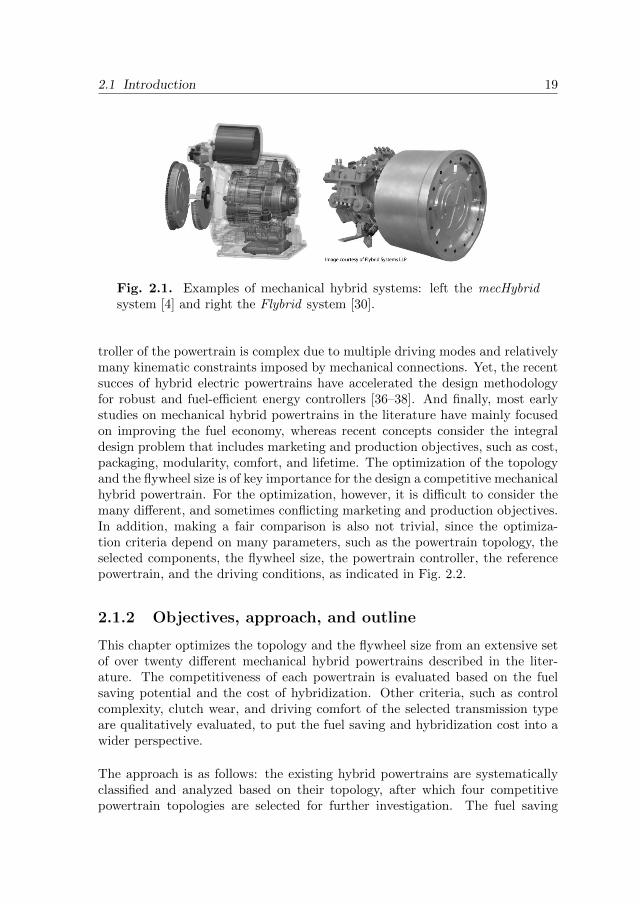
This research work focuses on mechanical hybrid powertrains that use a fly-wheel for energy storage and only mechanical components for power transmis-sion. The Continuously Variable Transmission (CVT) is usually selected for itssmooth shifting behavior, which allows for efficient energizing and de-energizingof the flywheel without energy conversion. The main advantage of mechanicalcomponents is that they are usually cheaper than equivalent high-power electriccomponents [5,7,28]. The energy storage capacity is relatively low, yet sufficientto recover the majority of the available brake energy [29]. The fuel saving ben-efits can be attributed to the added fuel saving functionalities: i) brake energyrecuperation for later use; ii) elimination of inefficient part-load operation of theengine; and iii) engine shutoff during vehicle standstill. These functionalitiesare especially effective during urban driving. The flywheel can also be used forboosting of the engine, yet the engine cannot be downsized due to the typicallylow energy storage capacity of the flywheel. Two examples of mechanical hybridsystems are shown in Fig. 2.1.
Flywheels have already been successfully applied to buses [31], trams [7], andFormula 1 racing cars [32]. Also, other applications have been proposed, such asfor commuter trains, cranes, forklift trucks, and excavators [7]. Except for theseniche applications, mass-production of mechanical hybrid passenger vehicles stillawaits due to several reasons. The commercially successful pushbelt CVT is arelatively young transmission technology (i.e., introduced in 1985 [33]), yet hasrecently grown towards a mature, low-cost and fuel-efficient technology [34],which is built in already 10% of the newly sold gasoline passenger vehicles [2].Accurate and robust control of clutches is complex due to dynamic operatingconditions and lack of torque sensors, yet recent developments in automatedtransmissions have shown viable solutions [27, 35]. The (optimal) energy con-
2.1 Introduction 19
Fig. 2.1. Examples of mechanical hybrid systems: left the mecHybridsystem [4] and right the Flybrid system [30].
troller of the powertrain is complex due to multiple driving modes and relativelymany kinematic constraints imposed by mechanical connections. Yet, the recentsucces of hybrid electric powertrains have accelerated the design methodologyfor robust and fuel-efficient energy controllers [36–38]. And finally, most earlystudies on mechanical hybrid powertrains in the literature have mainly focusedon improving the fuel economy, whereas recent concepts consider the integraldesign problem that includes marketing and production objectives, such as cost,packaging, modularity, comfort, and lifetime. The optimization of the topologyand the flywheel size is of key importance for the design a competitive mechanicalhybrid powertrain. For the optimization, however, it is difficult to consider themany different, and sometimes conflicting marketing and production objectives.In addition, making a fair comparison is also not trivial, since the optimiza-tion criteria depend on many parameters, such as the powertrain topology, theselected components, the flywheel size, the powertrain controller, the referencepowertrain, and the driving conditions, as indicated in Fig. 2.2.
2.1.2 Objectives, approach, and outline
This chapter optimizes the topology and the flywheel size from an extensive setof over twenty different mechanical hybrid powertrains described in the liter-ature. The competitiveness of each powertrain is evaluated based on the fuelsaving potential and the cost of hybridization. Other criteria, such as controlcomplexity, clutch wear, and driving comfort of the selected transmission typeare qualitatively evaluated, to put the fuel saving and hybridization cost into awider perspective.
The approach is as follows: the existing hybrid powertrains are systematicallyclassified and analyzed based on their topology, after which four competitivepowertrain topologies are selected for further investigation. The fuel saving

20 Chapter 2. Topology and flywheel size optimization
topology | size | control | components | reference | driver
hybridization cost
mass packaging
modularity
calibration
safety lifetime
fuel saving
control complexity
driveability
optimization criteria
emissions
design parameters
noise
criterion selected for optimization criterion influenced by selected criteria criterion not influenced by selected criteria
comfort
technology
Fig. 2.2. Schematic representation of the many design parameters andoptimization criteria. The selected optimization criteria cover an impor-tant share of the different and sometimes conflicting marketing and pro-duction objectives.
potential of each topology is computed with respect to the same conventionalpowertrain, for three certified driving cycles, using modular component modelsand an optimal energy controller, where the flywheel size is left as an optimiza-tion parameter. In this systematic approach, the design optimization problemwith multiple design parameters is reduced to solving a set of optimal controlproblems with different parameter settings, similar as done for hybrid electricpowertrains in [39], or for a turbocharger-assisted diesel engine in [40]. Thehybridization cost is estimated based on the type and size of the selected com-ponents. The remaining criteria are evaluated based on the simulation resultsand on the characteristics of the topology and transmission technology. Theresults give a qualitative understanding of the cost and benefits of each topol-ogy with different flywheel sizes, and quantifies the relative payback period andthe optimal flywheel size for each topology, thereby extending the earlier workpresented in [35].
The outline is given as follows: Section 2.2 presents the overview, classification,and selection of existing mechanical hybrid powertrain topologies. Section 2.3describes the modeling of the modular components and the selected powertrains.Section 2.4 defines the optimization problem. Section 2.5 describes the cost es-

2.2 Mechanical hybrid powertrain topologies in the literature 21
timation. The results are discussed in Section 2.6. Finally, the main conclusionsare given in Section 2.7.
2.2 Mechanical hybrid powertrain topologies inthe literature
The idea of using a flywheel for vehicle propulsion is not new. In the 1950s,the Gyrobus ran commercial service for several years using a flywheel to omitoverhead wire electrification between stops [31]. Since the 1970s, many flywheel-based hybrid vehicle concepts have appeared in the literature, where the flywheelis used to reduce the fuel consumption of passenger vehicles and buses. Sincethe 2000s, concepts for boosting performance are described for passenger vehi-cles and racing cars. The focus of this research work is to exploit the potentiallylow cost and high flywheel-to-vehicle efficiency of mechanical hybrid powertrainsfor the mainstream compact passenger vehicle segment, especially for emergingmarkets such as in China. Therefore, concepts using both a flywheel and bat-teries as described in [41, 42] are not considered for reasons of cost, whereasconcepts using a flywheel with an electric transmission as described in [7,43,44]are not considered due to the relatively low energy conversion efficiency. Con-cepts that only focus on boosting performance, such as during CVT shifts [5,45]or gear shifts [46, 47], are also not considered because of the limited fuel savingfunctionalities.
2.2.1 Classification
The remaining 18 concepts can be classified based on the topology of the mainpowertrain components, which are the Engine (E), Flywheel (F), Transmission(T), and Vehicle (V). In this abstraction, the transmission represents either anautomated gearbox or a CVT, whereas smaller components such as shafts, fixedgears, clutches, planetary brakes1, torque converters, and auxiliaries are not ex-plicitly shown, yet implied in the branches between the main components. As aresult, 7 different topology classes can be distinguished, as shown in Table 2.1.
The competitiveness of each class can be estimated qualitatively by comparisonof the different topology characteristics. The competitiveness is evaluated usingthree optimization criteria, which are the fuel saving, hybridization cost, andcontrol complexity. These criteria cover an important share of the relevant mar-keting and production objectives as schematically shown in Fig. 2.2. The fuelsaving is related to the reduced emission of pollutants and greenhouse gases, and
1A planetary brake uses a fixed disc brake on the ring branch of a planetary gear set tocontrol the torque transmission between the sun and carrier branches. Its functionality issimilar to that of a clutch in series with a fixed gear.

22 Chapter 2. Topology and flywheel size optimization
is influenced by the curb mass and the selected technology, e.g., the transmissiontype. The relative fuel saving can be estimated from the average transmission ef-ficiencies between the engine, flywheel, and vehicle, assuming that all topologiessupport the same fuel saving functionalities. The hybridization cost is relatedto the added mass, the selected technology, and the development effort for thepackaging (hardware) and the calibration (software). The relative hybridizationcost can be estimated from the number and type of transmission components.The control complexity is related to the functionalities and constraints of thetopology, which are influenced by requirements for driveability, comfort, noise,and lifetime. The relative control complexity can be estimated from the numberof driving modes and kinematic constraints.
In the series hybrid classes (S1,S2), the engine and flywheel are located in serieswith the vehicle. In this configuration, the flywheel is always connected to thevehicle while driving, so the flywheel speed may restrict the engine speed andits power capacity, which is not desired when driving on a highway or uphill ona slope. This problem can be solved by using a transmission on both sides ofthe flywheel (S1), so the engine speed can be controlled independently of theflywheel speed [48]. Alternatively, two transmissions can be used in series be-tween the flywheel and vehicle to create a very wide ratio coverage (S2), so theflywheel speed can be kept high for a wide vehicle velocity range, enabling ahigh engine speed and power at all times [49]. The main disadvantage of usingtwo transmissions in series, however, is the relatively low transmission efficiencyand the high cost.
In the parallel hybrid classes (P1-P5), the engine and flywheel are placed in par-allel, so each power source can be used individually for propulsion. Using a ded-icated transmission for each power source gives a high control degree of freedom,similar to that of parallel hybrid electric powertrains, allowing a variable speedratio between the flywheel and engine (P1,P2). The advantage with respect tothe series hybrid classes is that the engine-to-vehicle efficiency is unaffected whenthe flywheel is disengaged from the driveline. Also the cost of two transmissionscan be limited, by using a smaller (down-sized) CVT for the flywheel and alow-cost Automated Manual Transmission (AMT) for the engine, instead of arelatively expensive (normal-sized) CVT (see, Section 2.5). The driving comfortof an AMT, however, is less due to gear shifts with torque interruption. Onepossible configuration is to place the flywheel on the engine side of the maintransmission (P1), which gives a very wide flywheel-to-vehicle ratio coverage,but a low transmission efficiency [30, 50–52]. Placing the flywheel on the wheelside of the main transmission (P2) improves the flywheel-to-vehicle efficiency,but lowers the engine-to-flywheel efficiency to energize the flywheel [30,53–55].
The cost can be reduced further by using only one transmission (P3-P5). Placing

2.2 Mechanical hybrid powertrain topologies in the literature 23
Table 2.1. Classification of existing mechanical hybrid pow-ertrain topologies (E: engine, F: flywheel, T: transmission, andV: vehicle) and their estimated relative performance indices (−/ /+: worst/neutral/best).
class topology fuel cost control reference(s)
S1 E V T2 T1 F - - [48]
S2 E V T2 F T1 - - [49]
P1
E T1
F T2
V - + [30,50–52]
P2
E T1
F T2
V + [30,53–55]
P3
E T
F
V - + + [54]
P4
E T
F
V + [4, 56–58]
P5
E T
F
V + - [56, 59–61]
Si: Series class (i ∈ 1, 2). Pi: Parallel class (i ∈ 1, 2, 3, 4, 5).
the flywheel on the wheel side of the transmission (P3) requires a clutch or aplanetary brake between the flywheel and vehicle to transmit the demandedtorque while having a speed difference between the shafts, as the brake-hybridtopology of [54]. Such slipping components have a relatively low transmissionefficiency, yet the total system cost can be very low using only an AMT for theengine. The efficiency can be significantly improved by placing the flywheel onthe engine side of a (more costly) CVT (P4), at a higher control complexity dueto the fixed speed ratio between the engine and flywheel [4,56–58]. Adding a fewclutches to this configuration (P5), allows for more driving modes as describedin [56,59–61]. The many driving modes allow for many fuel saving functionalitiesusing only one transmission, but require a relatively complex controller.

24 Chapter 2. Topology and flywheel size optimization
V F
E V
F
E
V
F
E V
F
E
Brake Hybrid (base for topology 1)
Flybrid (base for topology 2)
mecHybrid (base for topology 3)
Flywheel Hybrid Drive II (base for topology 4)
Fig. 2.3. Selection of four competitive mechanical hybrid powertraintopologies. Each topology consists of an Engine (E), Flywheel (F), Vehicle(V), and dedicated transmission components.
2.2.2 Selection
The four most competitive topology classes in Table 2.1 (P2-P5), with the mainfocus on fuel saving and hybridization cost, are selected for further investigation.Of the P2 class, the Flybrid topology ( [30]) is selected, using an AMT with atorque converter for the engine and a small toroidal CVT with two clutches forthe flywheel. Of the P3 class, the Brake-Hybrid topology ( [54]) is selected, usingan AMT with a clutch for the engine and two planetary brakes for the flywheel.Of the P4 class, the mecHybrid topology ( [4]) is selected, using a CVT withthree clutches for both the engine and flywheel. Of the P5 class, the FlywheelHybrid Drive II topology ( [10]) is selected, using a CVT with five clutchesfor both the engine and flywheel. The powertrain topologies are schematicallydepicted in more detail with their dedicated transmission components in Fig. 2.3.
In the remainder of this chapter, the fuel saving potential and the hybridizationcost of each topology are computed using a set of modular component models.In this approach, it is necessary to scale and simplify the original transmissioncomponents to fit in the same framework. To clarify these (small) modifications,the names of the hybrid powertrain topologies are replaced by numbers, wherethe order denotes the control complexity from simple to complex: Brake-Hybrid(topology 1), Flybrid (topology 2), mecHybrid (topology 3), and Flywheel Hy-brid Drive II (topology 4).

2.3 Modeling 25
2.3 Modeling
The models describe the power flows (implicitly) as a function of the powerdemanded by the driving cycle. Besides power flows, kinematic relations mustbe taken into account, but are not explicitly described here. The dynamics aremodeled in a discrete forward Euler scheme using the time index “k” and afixed time step of ∆t = 1 s. The most relevant flywheel and vehicle inertias areconsidered, whereas smaller inertias such as that of the engine, clutches, gears,and pulleys are expected to have a negligible effect on the fuel consumption, andneglected to keep the number of states limited. For reasons of data availabilityand modularity, no distinction is made between a pushbelt CVT and a toroidalCVT as they share the same function, despite the difference in cost2. For thesame reasons, no distinction is made between a torque converter, clutch, and aplanetary brake, despite the torque amplification and the higher transmissionefficiency of the torque converter. As a result, the original topologies are slightlymodified from the ones described in the literature, resulting in the topologiesshown in Figs. (2.10)-(2.13).
The modeling of the power flows in the hybrid powertrain is separated into twolevels. The powertrain models describe the power balance between the com-ponents for different driving modes on a system level, whereas the componentmodels describe the power generation or power dissipation on component level.Two clutch types are distinguished to make this separation. The drive clutch hasconventional dimensions and is suitable to transmit high powers while slipping,e.g., when accelerating the vehicle from standstill, which may take several timesteps. The power dissipation of this clutch is modeled on component level in aclutch model. The mode clutch, on the other hand, is downsized to be just suffi-cient to select a driving mode φ on system level, by mechanical (dis-)engagementof powertrain parts, while dissipating only a limited amount of power and energy.It is assumed that the (dis-)engagement takes one time step, whereas the powerdissipation is negligible. In Figs. (2.10)-(2.13), the small clutches represent themode clutches, whereas the numbered large clutches represent the drive clutches.Before describing the modeling of each powertrain, the component models aredescribed in the sequel.
2.3.1 Components
The component models describe the power generation or power dissipation Pof each component as a function of the rotational speed ω and the transmittedtorque τ , and also as a function of the speed ratio for the CVT and AMT. Thespeed ratio r is defined as the output speed (superscript “out”) at the vehicle
2The toroidal CVT requires costly materials that can resist the relatively high stressesbetween the rollers and toroidal disks [62].

26 Chapter 2. Topology and flywheel size optimization
Table 2.2. Model parameters.
parameter value unit description
Ecrank 4.0 kJ engine cranking energy
Esync 2.0 kJ engine synchronization energymf 27 kg flywheel system massmv 1120 kg loaded vehicle massRw 0.281 m effective wheel radiusr1 1.10 - fixed gear 1 ratior4 2.50 - fixed gear 4 ratioramt 0.376, 0.797, 1.10, - AMT gear ratios
1.49, 1.92, 2.33rcvt [0.410, 2.32] - CVT speed ratiord 0.186 - final drive gear ratioβ 0.33 - brake power splitηe [0.00-0.36] - engine efficiency (see, Fig. 2.4)ηg [0.80-0.98] - gear efficiency (see, Fig. 2.6)ηamt [0.50-0.95] - AMT efficiency (see, Fig. 2.8)ηcvt [0.50-0.91] - CVT efficiency (see, Fig. 2.7)η1 0.99 - fixed gear 1 efficiencyη4 0.99 - fixed gear 4 efficiencyηd 0.98 - final drive efficiencyµsmall
cvt 0.84 - CVT downsize multiplierτe [0, 140] Nm engine torque (see, Fig. 2.4)τf [−100, 140] Nm flywheel torqueωe [0, 630] rad/s engine speedωe 105 rad/s minimum operation speedωf [105, 265] rad/s flywheel speedωidle 84 rad/s idling speed
side divided by the input speed (superscript “in”) at the power source side of thecomponent. The modeling data is obtained from the vehicle simulation platformAdvisor [63] and individual component experiments on a flywheel system [4]and a pushbelt CVT [64]. The semi-empiric power dissipation modeling of theflywheel system and CVT is extensively described in Appendix A, where it shownthat the average modeling error is less than 1% of the transmitted power. The setof realistic model parameters and their constraints are summarized in Table 2.2.
2.3.1.1 Engine
The internal combustion engine converts fuel into mechanical power throughcomplex chemical and mechanical processes. The mechanical power Pe is given

2.3 Modeling 27
by
Pe = ωeτe, (2.1)
where ωe denotes the rotational speed and τe the generated torque. For powergeneration (i.e., Pe > 0), the engine speed needs to exceed a minimum of ωe ≥ ωe
(105 rad/s). During engine idling (i.e., Pe = 0) with vehicle standstill (i.e.,vv = 0), the engine speed is reduced to ωe = ωidle (84 rad/s) for a lower fuelconsumption [65]. In the flywheel driving mode (φ = 1), the engine is shut-off,after which the engine speed quickly coasts down to ωe = 0 rad/s. The requiredfuel power Pf (i.e., chemical energy flux) at a given operating point (ωe, τe) isdescribed by a look-up table
Pf = Pf(ωe, τe). (2.2)
The mechanical efficiency of the engine ηe = Pe/Pf , based on static experimentswith a 4-cylinder 1.5-l 76-kW gasoline engine, is shown in Fig. 2.4. The enginecan be quickly cranked using the flywheel system, which is modeled as a powerdissipation for the flywheel system during one time step by
ωe [rad/s]
τ e[N
m] 35
33
31
2825
20
200 300 400 500 6000
50
100
150ηe [%]
Fig. 2.4. The mechanical efficiency ηe of a 4-cylinder, 1.5-l, 76-kW gaso-line internal combustion engine, as a function of the rotational speed (ωe)and the generated torque (τe).
Pcrank =
Ecrank
∆t if φ(k) 6= 1 ∧ φ(k − 1) = 1,
0 else,(2.3)
where Ecrank denotes the average cranking energy. When switching betweendriving modes φ while the engine remains switched on, the operating point of

28 Chapter 2. Topology and flywheel size optimization
the engine may substantially change. Dependent on the driving conditions,additional fuel is required to accelerate the engine inertia and to feed the pumpfor the actuation of the clutch(es) and the transmission. This fuel penalty tosynchronize the speeds in the powertrain is modeled as a power dissipation forthe engine during one time step by
Psync =
Esync
∆t if φ(k) 6= φ(k − 1) ∧ φ(k) 6= 1 ∧ φ(k − 1) 6= 1,
0 else,(2.4)
where Esync denotes the average synchronization energy. The energy penalties
Ecrank and Esync can be accurately modeled using a dynamic engine model,yet this is not necessary since the impact on the overall fuel consumption isrelatively small (1% − 2%). Instead, constant average values are considered,which are obtained from a more detailed simulation of the mechanical hybridpowertrain described in [66]. These energy penalties act as soft constraints on theassociated driving mode switches, such that “unnecessary” switches are avoided.Consequently, using these soft constraints, a better (qualitative) insight can beobtained in the flywheel utilization of each hybrid powertrain.
2.3.1.2 Flywheel system
The flywheel system contains a vacuum-placed steel rotor and a two-stage gearset to operate the rotor at high rotational speeds (up to 3140 rad/s). Thekinetic energy content of the rotor Er is determined by the rotor inertia and therotational speed by
Er =1
2Jrω
2f , (2.5)
where ωf denotes the rotational speed at the output shaft, Jr denotes the equiva-lent rotor inertia at this shaft, and the energy storage is limited Er ∈ [0, Er]. Forits purpose of urban driving, the speed range of the flywheel system is selected tomatch the engine speed range (between 105 and 265 rad/s) under normal urbandriving conditions, thereby facilitating a combined operation. For mechanicalhybrid vehicles, the energy storage capacity Er is the key sizing parameter toinfluence the fuel saving and the hybridization cost, in contrast to the powertransmission capacity for battery-based hybrid electric powertrains [39], so theflywheel system model must be scalable with Er. Assuming that the maximumallowed material stresses are utilized for the selected speed range and the givenrotor diameter, only the rotor height can be adapted to (proportionally) changethe energy storage capacity.

2.3 Modeling 29
The kinetic energy Er is controlled by the power exchange Pf with the remainderof the powertrain, and is affected by the storage losses in the rotor Pr and thetransmission losses in the gear set Pg. The dynamics is modeled by
Er(k + 1) = Er(k)− (Pf(k) + Pr(k) + Pg(k)) ∆t. (2.6)
The power dissipation in the rotor Pr is mainly caused by windage on the rotorsurface and friction in the bearings, which are typically functions of the speed ωf .Since the radial rotor surface dominates the windage losses [10] and the rotormass dominates the bearing load, the power dissipation scales approximatelyproportionally to the rotor height, hence also proportionally to Er. The scalablepower dissipation model is given by
Pr =Er
Enom
r
P nomr (ωf), (2.7)
where the nominal power dissipation model P nomr is obtained with coast-down
experiments using a steel rotor placed in a mild vacuum at its operating tem-perature, with a nominal energy storage capacity E
nom
r = 150 kJ, as shown inFig. 2.5. The power dissipation in the gear set Pg does not explicitly dependon the flywheel size, and is typically a function of the speed ωf and transmittedtorque τf . The power dissipation is modeled as a function of the transmissionefficiency ηg by
Pg =
(1
ηg(ωf ,τf )− 1)Pf if Pf > 0,
(ηg(ωf , τf)− 1)Pf else,(2.8)
where the efficiency model (ηg) is obtained with loaded experiments on a two-stage gear set with a total gear ratio of 1:11.8 and shown in Fig. 2.6. Theasymmetric efficiency is caused by an angle between the gear pairs, which re-sults in changing sliding forces between the gear teeth and normal forces on thebearings when the torque direction is switched.
2.3.1.3 Continuously variable transmission
The main components of the pushbelt CVT are the drive clutch, pump, variator,and final drive, where the variator enables a continuously variable speed ratiorcvt. The power dissipation in the CVT includes the power consumption of thepump and the power dissipation in the clutch, variator, and final drive. Thepower dissipation in the drive clutch and the final drive, however, are modeledseparately to obtain a higher modularity of the component models. The resulting

30 Chapter 2. Topology and flywheel size optimization
ωf [rad/s]
Pnom
r[W
]
0 50 100 150 200 2500
50
100
150
200
250
Fig. 2.5. Semi-empirical power dissipation model of the rotor (Pr) as afunction of the speed at the output shaft (ωf) as described in Appendix Abased on experiments on a 150-kJ flywheel system, as described in Ap-pendix A
ωf [rad/s]
τ f[N
m]
9897
95
85
95
85
100 120 140 160 180 200 220 240 260−100
−50
0
50
100ηg [%]
Fig. 2.6. Semi-empirical power transmission efficiency model of the gearset (ηg) as a function of the speed (ωf) and the torque at the output shaft(τf) based on 35-kW flywheel system, as described in Appendix A.
power dissipation model Pcvt can be described as a function of the transmissionefficiency ηcvt by
Pcvt =
(1
ηcvt(ωoutcvt ,τ
outcvt ,rv)
− 1)τoutcvt ω
outcvt if τout
cvt ωoutcvt > 0,
(ηcvt(ωoutcvt , τ
outcvt , rv))− 1) τout
cvt ωoutcvt else,
(2.9)
where the transmission efficiency (ηcvt) is described by a semi-empirical modelbased on loaded experiments on a 76-kW mass-produced CVT, as a function

2.3 Modeling 31
of the speed ωoutcvt , the transmitted (positive, or negative) torque τout
cvt , and thespeed rcvt [64, 67]. The transmission efficiency including the final drive (ηcvtηd)is shown in Fig. 2.7.
ωoutcvt [rad/s]
τout
cvt
[Nm
]
9088
8580
70
8885
8070
100 200 300 400 500 600
−100
−50
0
50
100 ηcvtηd [%]
(a) Constant speed ratio of rcvt = 1.
ln(rcvt) [-]
τout
cvt
[Nm
]
7080
8588
90
7080
85 88
−0.8 −0.6 −0.4 −0.2 0 0.2 0.4 0.6 0.8−150
−100
−50
0
50
100
150 ηcvtηd [%]
(b) Constant input speed ωincvt = 100 rad/s.
Fig. 2.7. Semi-empirical power transmission efficiency of the CVT in-cluding final drive ηcvtηd, as a function of the output torque τout
cvt , outputspeed ωout
cvt , and speed ratio rcvt based on a 76-kW pushbelt CVT, asdescribed in Appendix A.
For the smaller 35-kW CVT used in topology 2, a higher efficiency is expectedwith a smaller pump, yet this effect is limited by other frictional, slip, andchurning losses [34]. Without considering the compliances of a detailed effi-ciency model, this higher efficiency potential is modeled by a constant multiplierµsmall
cvt = 0.7 + 0.3(35/76) ≈ 0.84, which represents a proportional improvementof the smaller pump that counts for thirty percent of the total power dissipation.The power dissipation of the downsized CVT P small
cvt is then given by

32 Chapter 2. Topology and flywheel size optimization
P smallcvt = µsmall
cvt Pcvt. (2.10)
2.3.1.4 Automated manual transmission
The main components of the AMT are the drive clutch, pump, gearbox, andfinal drive, where the gear box enables six different gear ratios ramt. The up-coming 6-speed AMT is selected rather than the currently more common 5-speedAMT [2], which matches better with the wide ratio coverage of the CVT. Thepower dissipation in the AMT includes the power consumption of the pump andthe power dissipation in the clutch, gearbox, and the final drive. The power dis-sipation in the drive clutch and the final drive, however, are not included in theAMT model, yet modeled separately to obtain a higher modularity of the com-ponent models. The resulting power dissipation model Pamt can be described asa function of the transmission efficiency ηamt by
Pamt =
(1
ηamt(ωoutamt, τ
outamt, ramt
− 1
)τoutamtω
outamt, (2.11)
where the transmission efficiency (ηamt) is described by an empirical model takenfrom Advisor [63, 68], as a function of the speed ωout
amt, the transmitted torqueτoutamt, and the speed ratio ramt. The transmission efficiency including the final
drive (ηamtηd) is shown in Fig. 2.8.
ωoutamt [rad/s]
τout
am
t[N
m]
94
92
90
85
70
100 200 300 400 500 6000
20
40
60
80
100
120
140ηamtηd [%]
Fig. 2.8. Empirical power transmission efficiency of the AMT includingfinal drive ηamtηd as a function of the output speed ωout
amt and outputtorque τout
amt, for the third gear (ramt = 1.098), generated with data fromAdvisor [63,68].

2.3 Modeling 33
2.3.1.5 Drive clutch
The drive clutch can accelerate the vehicle from standstill by friction between theslipping clutch plates. When engaged, the clutch can transmit torque in eitherdirection with virtually no power dissipation. When slipping, the pressure forceon the clutch plates can be manipulated by a hydraulic actuator to control thetransmitted clutch torque τc. The torque is transmitted from the high-speedside to the low-speed side of the clutch, so sign(τc) = sign(ωin
c − ωoutc ). The
associated power dissipation is modeled by
Pc = τc(ωinc − ωout
c ). (2.12)
Due to relatively high power dissipation on a relatively small slipping surface,local temperature peaks may substantially shorten the lifetime of the clutch.The impact of the powertrain topology on the thermal load of the clutch will bediscussed with supportive simulation results in Section 2.6.1.
2.3.1.6 Fixed gear
Fixed gears are as used as the final drive (subscript “d”) to the wheels in eachtopology, and additionally in topology 1 (subscript “1”) and in topology 4 (sub-script “4”). The speed ratio rd is fixed for all topologies, whereas r1 and r4
are tuned for high fuel savings for the associated topology, considering variousflywheel sizes. Since the power dissipation of the fixed gears are relatively lowcompared to that of other components, constant (average) efficiencies can beconsidered without affecting the fuel economy significantly. The resulting powerdissipation model Pi (i ∈ d, 1, 4) can be described as a function of the averagetransmission efficiency ηi by
Pi =
( 1ηi− 1)P out
i if P outi ≥ 0,
(ηi − 1)P outi else.
(2.13)
2.3.1.7 Vehicle
The vehicle tracks the velocity vv and acceleration av profiles prescribed by thedriving cycle. The considered driving cycles have, as the majority of the drivingcycles described in the literature, no variations in altitude, wind, or road surface.The wheel shaft speed is related to the vehicle velocity by the effective wheelradius Rw, thereby neglecting any wheel slip. The vehicle propulsion or brakingpower Pv is given by
Pv = (1− β)(mvavvv + Fv(vv)vv), (2.14)

34 Chapter 2. Topology and flywheel size optimization
wheremv is the equivalent mass of the vehicle with two passengers and the inertiaof the wheels, where other (minor) powertrain inertias are neglected. The termFv describes the combined rolling and aerodynamic force as a function of thevehicle velocity (vv). The braking power is partly recuperated by the flywheelsystem, and partly dissipated by the conventional disc brakes, where a constantrelative brake power split of β = 0.33 is assumed during regenerative braking.Lower brake power split factors are possible (up to 0.062) within European safetyregulations [69], yet require a costly certified brake-blend system that interveneswith the conventional brake system [70] to gain only a few percent fuel saving.Brake energy recuperation is only supported in the flywheel driving mode (φ = 1)if the flywheel system is not saturated (Er < Er), so
β =
0 if (mvavvv + Fv(vv)vv) ≥ 0,
0.33 else if φ = 1 ∧ Er < Er,
1 else.
(2.15)
2.3.2 Powertrains
The modular component models are used to compose the four selected hybridpowertrain models and a conventional powertrain model as a reference. Thepower dissipation of each drive clutch Pc,i is numbered conform the numbersi ∈ 1, 2, 3 shown in Figs. 2.9-2.13. Since each hybrid powertrain uses thesame final drive and disc brakes, these components are not explicitly shown butimplied in the vehicle model (V). For the same reason, the rotor and gears setare implied in the flywheel system model (F). For each powertrain, the powerbalance of the flywheel system and engine can be described as a function of thedriving mode. In general, each of the hybrid powertrains can be operated in thesame driving modes:
• Flywheel driving : the flywheel system propels or brakes the vehicle, whilethe engine is disengaged and shut-off (φ = 1).
• Hybrid driving : the engine propels the vehicle and energizes the flywheelat an efficient operating point, where the power split Pu determines thepower distribution (φ = 2).
• Engine driving : the engine propels the vehicle, while the flywheel systemis disengaged and coasting, (φ = 3).
Topology 4 supports additional modes for hybrid driving (φ = 4) and enginedriving (φ = 5), both with higher speed ratios between the engine and driveshaft to enable lower engine speeds for a lower fuel consumption. An additionaldriving mode is possible for topologies 3 and 4, which energizes the flywheelwith the engine during vehicle standstill, but is not supported as it does not

2.3 Modeling 35
improve the fuel consumption and produces an uncomfortable and unexpectedengine noise.
2.3.2.1 Conventional powertrain
The distinguishing components are the AMT and drive clutch, as schematicallyshown in Fig. 2.9. For this reference powertrain, the AMT is selected to separatethe effects of hybridization from the effects of automatization without addingmuch cost. This powertrain supports only engine driving (φ = 3), which isdescribed by:
φ = 3⇐⇒ Pe = Pv + Pamt + Pc,1. (2.16)
1
E V AMT
engine driving (φ=3)
Fig. 2.9. Schematic representation of the conventional (reference) pow-ertrain topology.
2.3.2.2 Hybrid powertrain topology 1
The distinguishing components are an AMT, three drive clutches and an addi-tional fixed gear, as schematically shown in Fig. 2.10. Although one drive clutch(e.g., clutch 2) on the flywheel system shaft would be sufficient for the samefunctionalities, a second drive clutch is added for a better heat distribution ofthe dissipated energy, cf. the original design with two planetary brakes [54] (see,Fig. 2.3). The three driving modes are flywheel driving (φ = 1), hybrid driv-ing (φ = 2), and engine driving (φ = 3), where Pu determines the power splitbetween the power sources for φ = 2:
φ = 1⇐⇒Pe = 0,Pf = Pv + Pc,3 + P1 + Pc,2,
(2.17)
φ = 2⇐⇒Pe = Pv + Pamt + Pc,1 + Psync + Pu,Pf = Pc,3 + P1 + Pc,2 + Pcrank − Pu,
(2.18)
φ = 3⇐⇒Pe = Pv + Pamt + Pc,1 + Psync,Pf = Pcrank.
(2.19)

36 Chapter 2. Topology and flywheel size optimization
1
V
F
AMT
E 2 3
flywheel driving (φ=1) hybrid driving (φ=2) engine driving (φ=3)
Fig. 2.10. Schematic representation of hybrid powertrain topology 1.
2.3.2.3 Hybrid powertrain topology 2
The distinguishing components are an AMT, a small CVT, two drive clutches,and one mode clutch, as schematically shown in Fig. 2.11. This topology sup-ports the same driving modes as topology 1 using different components:
φ = 1⇐⇒Pe = 0,Pf = Pv + P small
cvt + Pc,2,(2.20)
φ = 2⇐⇒Pe = Pv + Pamt + Pc,1 + Psync + Pu,Pf = P small
cvt + Pc,2 + Pcrank − Pu,(2.21)
φ = 3⇐⇒Pe = Pv + Pamt + Pc,1 + Psync,Pf = Pcrank.
(2.22)
V
F
AMT
small CVT
E
flywheel driving (φ=1) hybrid driving (φ=2) engine driving (φ=3)
1
2
Fig. 2.11. Schematic representation of hybrid powertrain topology 2.

2.3 Modeling 37
2.3.2.4 Hybrid powertrain topology 3
The distinguishing components are a (normal) CVT, one drive clutch, and twomode clutches, as schematically shown in Fig. 2.12. This topology supports thesame driving modes as topologies 1 and 2, using different components:
φ = 1⇐⇒Pe = 0,Pf = Pv + Pcvt + Pc,1,
(2.23)
φ = 2⇐⇒Pe = Pv + Pcvt + Pc,1 + Psync + Pu,Pf = Pcrank − Pu,
(2.24)
φ = 3⇐⇒Pe = Pv + Pcvt + Pc,1 + Psync,Pf = Pcrank.
(2.25)
1
V
F
CVT
E
flywheel driving (φ=1) hybrid driving (φ=2) engine driving (φ=3)
Fig. 2.12. Schematic representation of hybrid powertrain topology 3.
2.3.2.5 Hybrid powertrain topology 4
The distinguishing components are a CVT, two drive clutches, three modeclutches, and an additional fixed gear, as schematically shown in Fig. 2.13.This topology supports five driving modes, which are low-speed flywheel driving(φ = 1), low-speed hybrid driving (φ = 2), low-speed engine driving (φ = 3),high-speed hybrid driving (φ = 4), and high-speed engine driving (φ = 5), wherePu determines the power split between the power sources for φ = 2 and φ = 4:
φ = 1⇐⇒Pe = 0,Pf = Pv + Pcvt + Pc,2,
(2.26)
φ = 2⇐⇒Pe = Pv + Pcvt + Pc,1 + Psync + Pu,Pf = Pc,2 + Pcrank − Pu,
(2.27)
φ = 3⇐⇒Pe = Pv + Pcvt + Pc,1 + Psync,Pf = Pcrank,
(2.28)
φ = 4⇐⇒Pe = Pv + P4 + Psync + Pu,Pf = Pcvt + Pc,1 + Pcrank − Pu,
(2.29)
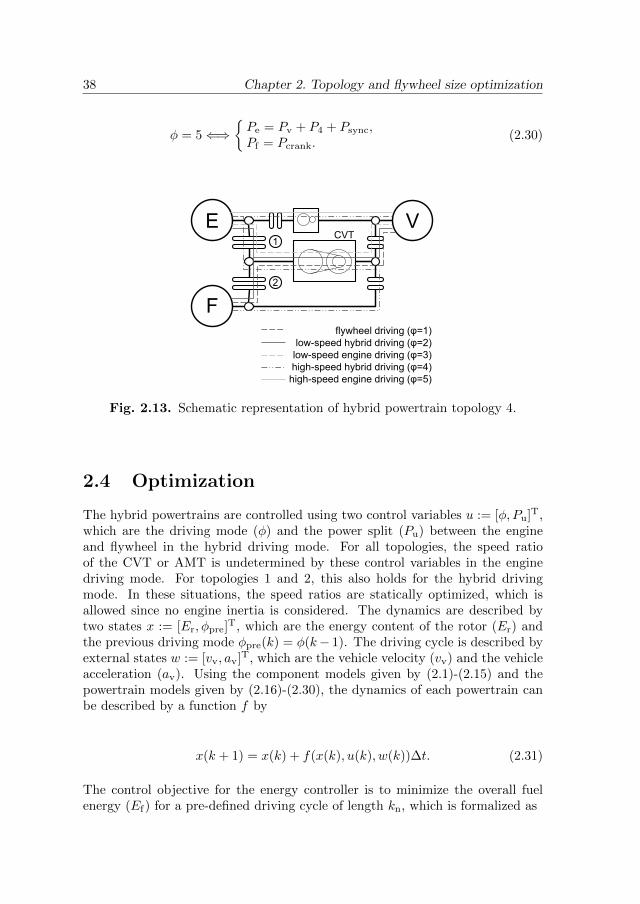
38 Chapter 2. Topology and flywheel size optimization
φ = 5⇐⇒Pe = Pv + P4 + Psync,Pf = Pcrank.
(2.30)
V
F
CVT E
flywheel driving (φ=1) low-speed hybrid driving (φ=2)
low-speed engine driving (φ=3) high-speed hybrid driving (φ=4) high-speed engine driving (φ=5)
2
1
Fig. 2.13. Schematic representation of hybrid powertrain topology 4.
2.4 Optimization
The hybrid powertrains are controlled using two control variables u := [φ, Pu]T,which are the driving mode (φ) and the power split (Pu) between the engineand flywheel in the hybrid driving mode. For all topologies, the speed ratioof the CVT or AMT is undetermined by these control variables in the enginedriving mode. For topologies 1 and 2, this also holds for the hybrid drivingmode. In these situations, the speed ratios are statically optimized, which isallowed since no engine inertia is considered. The dynamics are described bytwo states x := [Er, φpre]T, which are the energy content of the rotor (Er) andthe previous driving mode φpre(k) = φ(k− 1). The driving cycle is described byexternal states w := [vv, av]T, which are the vehicle velocity (vv) and the vehicleacceleration (av). Using the component models given by (2.1)-(2.15) and thepowertrain models given by (2.16)-(2.30), the dynamics of each powertrain canbe described by a function f by
x(k + 1) = x(k) + f(x(k), u(k), w(k))∆t. (2.31)
The control objective for the energy controller is to minimize the overall fuelenergy (Ef) for a pre-defined driving cycle of length kn, which is formalized as

2.5 Cost estimation 39
minu(k)
kn−1∑k=k0
Pf(x(k), u(k), w(k))∆t, (2.32)
subject to the physical operating limits as listed in Table 2.2, the dynamicsdescribed by (2.31), the kinematic relations given by the speed ratios of thegears and transmissions, and the final state constraint
Er(kn) ≥ Er(k0) (2.33)
for a fair comparison between the different topologies and flywheel sizes. Thepowertrains start under “warm” conditions, where the powertrain is alreadyat operating temperature, the flywheel system contains 50% of its capacityEr(k0) = 0.5Er, and the hybrid powertrain is in flywheel driving mode φ(k0) = 1.The optimal control problem is solved for a set of three driving cycles, whichare the New European Driving Cycle (NEDC), the Japan Cycle 08 (JC08), andthe Federal Test Procedure ’75 (FTP75). These driving cycles represent mixedurban and highway driving conditions that are used for certified fuel consump-tion measurements in relevant continents of the automotive industry, i.e., Asia,Europe, and North-America. Since the flywheel system is aimed for urban used,no highway-only cycles are considered.
Deterministic dynamic programming is used to solve this optimal control prob-lem, which is a suitable numerical method to deal with the switched, non-lineardynamics and the relatively many constraints [18]. The solution is optimal inthe sense of achievable optimality, despite approximation errors introduced bymathematical modeling and numerical quantization. The continuous optimalcontrol problem is implemented in the discrete framework using a computation-ally efficient implementation method that avoids nearest-neighbor rounding ofthe state trajectories, as described in [71]. The continuous energy state (Er)is quantized with a resolution of 1500 kJ, whereas the continuous power splitcontrol variable (Pu) is quantized into 20 evenly distributed values between its(state-dependent) extrema.
2.5 Cost estimation
Cost estimation of the powertrain components is difficult, because detailed in-formation from the industry is scarce and prices are subject to change. On theother hand, even a rough cost estimation can put the investigated topologiesinto perspective and give qualitative insights. A rough estimation of the costis composed using weight-specific quantities as in [5, 7]. The mass of the power

40 Chapter 2. Topology and flywheel size optimization
Table 2.3. Production cost and consumer cost estimation.
transmission power specific component specific consumercomponents capacity mass mass cost cost
[kW] [kg/kW12 ] [kg] [€/kg] [€]
AMT1 76 4.8 42 10 837CVT1 35, 76 6.5 38, 57 13 1000, 1473drive clutch 76 0.6 5.2 14 146mode clutch 35 0.6 3.5 12 85flywheel gear set 35 1.4 8.3 14 232fixed gear 76 0.2 1.7 12 42adaptations - - - - 120
storage energy specific component specific consumercomponents capacity mass mass cost cost
[kJ] [kg/kJ] [kg] [€/kg] [€]
rotor 25-250 0.065 1.6-16.3 7 23-228housing 25-250 0.035 0.9-8.8 8 14-140
1excluding drive clutch, including final drive.
transmission components is scaled with the square root of the power capacity,based on observations in [3]. The relative quantities of the AMT and CVT arederived from [3], where it is assumed that the mass of a 6-speed AMT is 20%higher than that of a (non-automated) 5-speed manual transmission, due to theadditional actuation system (including pump), additional gear, and larger hous-ing. The relative masses and specific costs of the flywheel-related componentsare based on estimations carried out for the mecHybrid components [4] and in-clude all required parts such as actuation, suspension, and lubrication systems,where a (mass-)production volume of over 100, 000 units per year is assumed.All components are (mainly) made of steel, except for the housing (aluminum),with a varying weight-specific cost that depends on the complexity of the ma-chine operations and the number of required parts and actuation systems. Afixed cost is assumed for an additional control unit for the flywheel system andminor vehicle adaptations. The estimated production costs are multiplied bya factor of 2 to give an indication of the consumer costs. The resulting costestimates are listed in Table 2.3.
2.6 Results and discussion
The results of the fuel consumption optimization and the cost estimation arecompared to find the optimal powertrain topology and the associated optimal

2.6 Results and discussion 41
flywheel size. Other criteria, such as control complexity, clutch wear, and thedriving comfort are qualitatively evaluated, to put the fuel saving and hybridiza-tion cost into a wider perspective.
2.6.1 Topology optimization
Fig. 2.14 shows an overview of the reduced fuel consumption and the hybridiza-tion cost of the four hybrid powertrain with respect to the conventional pow-ertrain, for the three driving cycles. For each topology, various flywheel sizesEr ∈ 25, 50, 75, 100, 150, 200, 250 kJ are shown, which are linearly related tothe hybridization cost, i.e., the smallest flywheel size corresponds to the markerwith the lowest cost. Before discussing the impact of the flywheel size on theoptimization criteria in the sequel, the impact of the topology is discussed. Itcan be observed that topology 1 has despite the high energy dissipation in theclutches, a relatively high fuel saving potential (14% − 25%) at the lowest cost(€730-€1050). Topologies 2-4 have even a higher fuel saving potential due to thehigher transmission efficiencies, but also at a higher cost due to the use of moreexpensive components. From these topologies, topology 2 has the lowest fuelsaving (19% − 34%) due to the relatively low engine-to-flywheel efficiency, butthe highest cost (€1620-€1950) due to the use of two transmissions. Topology3 has a very high engine-to-flywheel efficiency and uses only one transmission,which results in a higher fuel saving (22%−37%) at a lower cost (€1200-€1530),but requires a more complex controller design due to the mechanical connectionbetween the engine and flywheel. Topology 4 achieves the highest fuel saving(28% − 39%) at a slightly higher cost (€1480-€1800), but also with the mostcomplex controller design because of many kinematic constraints and the rela-tively many driving modes.
In general, it is observed that the investigated topologies have approximatelythe same ratio between the fuel saving and the hybridization cost, with a least-square fit of -0.0189 %/€(or, 53 €/%). This ratio can be related to an econom-ically attractive payback period of the investment, as will be explained in thesequel. From this point of view, topologies 1, 3, and 4 show a similar competi-tiveness, whereas topology 2 is somewhat less competitive. To put the paybackperiod into a wider perspective, other criteria must be considered as well, suchas expected lifetime issues, control complexity, and driving comfort. For allconsidered topologies, the drive clutch(es) is more frequently used at a higherthermal load, which may become critical for the lifetime of this component. Thethermal load is especially high for topology 1, which uses slipping drive clutchesfor power transmission between the flywheel system and vehicle, as will be dis-cussed in more detail in the sequel. In order to guarantee a high driving comfort,each driving mode switch must be performed quickly, consistent, and withouttorque interruption, or circumvented otherwise, which is a challenging control

42 Chapter 2. Topology and flywheel size optimization
consumer cost [euro]
fuel
consu
mption
[%]
600 800 1000 1200 1400 1600 1800 2000
−40
−35
−30
−25
−20
−15
−10
topology 1topology 2topology 3topology 4-0.0189 %/euro
NEDCFTP75JC08
Fig. 2.14. The relative fuel consumption as a function of the consumercost of hybridization, shown for the four hybrid topologies with respectto the conventional topology. The markers denote different flywheel sizes,whereas the lines denote different driving cycles. The relative fuel con-sumption is computed as the difference in the overall fuel consumption(Ef) with respect to that of the conventional powertrain. The hybridiza-tion cost is computed as the difference in the consumer cost of the hybridtopology with respect to that of the conventional topology.
task. The control complexity is related to the number of driving mode switchesand kinematic constraints, as discussed in Section 2.2, which is indicated by thetopology numbering. Despite the different levels of complexity, similar controlchallenges must be solved for each topology. Assuming that these challengesare solvable, the driving comfort is expected to be higher for topologies 3 and4 than for topologies 1 and 2, due to the smooth shifting behavior of the CVT,in contrast to the torque interrupted gear shifts of the AMT. A dual clutchtransmission could replace the AMT for a higher driving comfort, but at a sig-nificantly higher cost [3]. Considering the longer payback period of topology 2,the clutch lifetime concerns and the lower driving comfort of topology 1, andthe control complexity of topology 4, topology 3 is expected to be the mostcompetitive of the considered topologies.
The use of mechanical components for hybridization is especially cost-effectivewhen standard components can be used. Standard transmissions are suitablefor the hybrid powertrains, as these are operated in the same speed and torquerange as for the conventional powertrain during propulsion. The standard CVTis also suitable for regenerative braking [64], whereas the AMT is not used forthis functionality. The use of standard drive clutches, however, may require fur-ther investigation due to the more frequent usage at a higher thermal load. The

2.6 Results and discussion 43
thermal load is a critical quantity for the lifetime of a clutch, which depends onthe momentary power dissipation, the total energy dissipation, and the trans-mission cooling capacity [72]. Fig. 2.15 shows for each hybrid powertrain witha 150-kJ flywheel system, the relative maximum power dissipation (top graph)and the relative total energy dissipation (bottom graph) of the combined driveclutches in the powertrain, with respect to that of the (single) drive clutch of theconventional topology. As can be seen, all hybrid topologies have a substantiallyhigher power peak (on average a factor 1.7) and energy dissipation (on averagea factor 2.8) than the conventional powertrain. This is partly due to the veryefficient drive clutch usage of the conventional powertrain, as the vehicle is oftenaccelerated from standstill with the minimal engine speed of 105 rad/s. A morerealistic engine speed of 150 rad/s-200 rad/s would reduce the relative power andenergy dissipation shown in Fig. 2.15 by approximately a factor 1.5-2, and re-semble better with the speed range of the flywheel system (i.e., [105, 265] rad/s).Then, the thermal loads of topologies 2-4 are close to that of the conventionalpowertrain, but topology 1 still has a significantly higher thermal load. For thisreason, topology 1 is equipped with two drive clutches on the flywheel system(see, Fig. 2.10) shaft for a better heat distribution, but the total cooling capac-ity may still be challenging within a compact and low-cost hybrid powertraindesign.
max
imum
pow
er[%
]
0
100
200
300
400NEDCFTP75JC08
tota
len
ergy
[%]
topology # [-]1 2 3 4
0
200
400
600
Fig. 2.15. The relative maximum power dissipation and the relativetotal energy dissipation of the combined drive clutches for each hybridtopology (equipped with a 150-kJ flywheel) with respect to that of theconventional powertrain.

44 Chapter 2. Topology and flywheel size optimization
2.6.2 Flywheel size optimization
For mechanical hybrid vehicles, the energy storage capacity is the key sizingparameter to influence the fuel consumption and the hybridization cost, in con-trast to the power transmission capacity for hybrid electric powertrains. FromFig. 2.14 it can be seen that, in general, the fuel consumption decreases with theflywheel size due to less limitations on brake energy recuperation and less driv-ing mode switches. From a certain flywheel size, however, the negative impactof higher drag losses and a smaller dynamic speed range of the flywheel systembecomes dominant, resulting in an increasing fuel consumption. More detailedresults are given in Fig. 2.16.
pay
bac
kper
iod
[%]
40
50
60
70
energy storage capacity [%]
mode
switch
es[%
]
40 60 80 100 120 140 160 180 200100
150
200
250 topology 1topology 2topology 3topology 4
Fig. 2.16. The impact of the relative flywheel size on the relative paybackperiod (top graph) and the relative number of driving mode switches(bottom graph).
The top graph of Fig. 2.16 shows the relative payback period3 for the combinedthree driving cycles as a function of the relative flywheel size. The relativepayback period of the hybrid powertrain quantifies the fuel saving benefit withrespect to the hybridization investment and the service life4 of passenger vehi-cles. The fuel consumption benefit is computed with a gasoline price of €1.538per liter (average in Europe, April 2013) and an energy density of 32.2 MJ/l. Therelative flywheel size is defined as the energy storage capacity with respect to the
3Relative payback period [%] = 100 [%] × hybridization cost [€]/(fuel saving [l/km] × fuelprice [€/l] × service life [km])
4The service life of passenger vehicles equals 150,000 km as defined in [3].

2.6 Results and discussion 45
kinetic vehicle energy at an urban vehicle velocity of 13.9 m/s (50 km/h), whichcan be related to the brake energy recuperation possibilities in urban traffic. Fortopology 1, the lowest relative payback period is obtained with a relative fly-wheel size of 40%, whereas for topologies 2-4, the lowest relative payback periodis obtained with a relative flywheel size of 60%. When considering the differenttransmission efficiencies of each topology, it appears that the optimal flywheelsize is able to recover the majority (80% − 100%) of the brake energy duringurban driving, which supports the results in [29]. Since the payback period isrelatively insensitive to the flywheel size around its minimum, a somewhat largerflywheel size can be selected to significantly reduce the number of driving modeswitches.
The bottom graph of Fig. 2.16 shows the relative number of driving modeswitches for the combined three driving cycles as a function of the relative fly-wheel size, where the largest flywheel size of 200% is considered as the reference.The number of driving mode switches is related the lifetime of the mode clutchesand variations in the engine speed that result from duty-cycle switching betweenhybrid and flywheel driving. As expected, the number of driving mode switchesdecreases with the flywheel size, where this effect gradually reduces for largerflywheel sizes. It is seen that topologies 2-4 show similar characteristics, due tothe similar utilization of the flywheel system. The characteristic of topology 1,on the other hand, is much less sensitive to the flywheel size, as the flywheelsystem is mainly used to recuperate brake energy, which is used to propel thevehicle immediately afterwards. The flywheel size has only a limited impact onthe number of driving mode switches using this control strategy.
2.6.3 The potential of mechanical hybrid powertrains
With the relatively small differences between the investigated topologies, it isconcluded that mechanical hybrid powertrains in general have the potential to beeconomically attractive. The fuel saving benefit returns the hybridization invest-ment well within (39%−62%) the service life of passenger vehicles, even without(direct) incentives by the government. The payback period becomes even moreattractive when anticipating increasing fuel prices [1] and a longer utilization ofthe passenger vehicles than the service life of 150,000 km. When considering,for topologies 3 and 4, the same CVT in the reference powertrain (instead of theAMT), the relative payback period even reduces to 21% − 26%. However, it isimportant to realize that these results are optimistic as the fuel saving is basedon optimal control, warm start conditions, and without constraints on possiblyuncomfortable driving mode switches. One of the main challenges is the designof a powertrain controller, suitable for implementation in real-time hardware,that controls the energy dynamics with a close-to-optimal fuel economy perfor-

46 Chapter 2. Topology and flywheel size optimization
mance, and the torque dynamics with a quick, smooth, and consistent responsefor all driving modes and driving mode switches.
Although the conventional performance remains unaffected (i.e., engine driv-ing mode), the consumer may expect a higher acceleration performance froma hybrid powertrain. For this market segment, the mechanical hybrid power-train could serve as a low-cost basis that is extendable with a small electricpower source for boosting performance, e.g., by combining the favorable powercapacity of the flywheel system with the favorable energy storage capacity ofthe batteries, and the favorable controllability of the electric machine. Addingthese design dimensions, however, substantially complicates the integral designoptimization of the hybrid powertrain as argued, e.g., in [23].
2.7 Conclusions
This chapter has optimized the topology and the flywheel size of a mechanicalhybrid powertrain, from an extensive set of over twenty different concepts de-scribed in the literature. The competitiveness of each powertrain is evaluatedbased on the fuel saving potential and the cost of hybridization with respectto a conventional powertrain. Three of the considered topologies have a verycompetitive ratio between the fuel saving and hybridization cost, which canbe quantified as a relative payback period between 39% − 45% of the servicelife of passenger vehicles. When considering also other criteria, such as controlcomplexity, clutch wear, and driving comfort are qualitatively evaluated, to putthe fuel saving and hybridization cost into a wider perspective, the mecHybridtopology described in [4] is expected to be the most competitive. The associatedoptimal energy storage capacity of the flywheel is equivalent to the kinetic energyof the vehicle during urban driving (50 km/h), which is one of the key function-alities of mechanical hybrid powertrains. Due to the relatively small differencesbetween the investigated topologies, however, it is concluded that mechanicalhybrid powertrains in general have the potential to be economically attractive.This is especially the case for the CVT-based hybrid powertrains, which alsoimprove the driving comfort with respect to the AMT-based conventional pow-ertrain. One of the main challenges for mechanical hybrid powertrains, however,is the design of a real-time powertrain controller that guarantees a low overallfuel consumption and a quick, smooth, and consistent torque response.

Chapter 3
Optimal energy control withcomfort related constraints
Abstract – This chapter presents the modeling and the design of an optimal energy controller
for a mechanical hybrid powertrain. The powertrain is characterized by i) switched dynamics
due to discrete driving modes; ii) active state constraints, due to the relatively small energy
storage capacity of the flywheel system and the mechanical connection between the engine and
the flywheel system; and iii) non-convex control constraints to avoid uncomfortable driving
mode switches. The optimization problem is to find the optimal sequence of driving modes
and power splits between the engine and the flywheel system, that minimizes the overall fuel
consumption for a pre-defined driving cycle. This relatively complex optimization problem
is solved using deterministic dynamic programming, for six representative and diverse driv-
ing cycles. The optimal solution provides a benchmark of the fuel saving potential for this
mechanical hybrid powertrain, and gives insights in the impact of the added functionalities,
in the increased transmission losses, and in the optimal powertrain utilization. Results show
that very high fuel savings can be obtained of between 20% − 40%, dependent on the driving
cycle, where each fuel saving functionality contributes with a significant amount to the fuel
saving potential. In addition, it is shown that the optimal control problem can be substantially
reduced, by reducing the power split control space to only two essential values with only a
negligible impact (< 0.4%) on the fuel saving.
3.1 Introduction
Hybrid powertrains have the potential to significantly improve the fuel econ-omy of passenger vehicles by adding a secondary power source to the internalcombustion engine. Commercially available hybrid electric powertrains showpromising fuel savings, but at a relatively high cost due to the use of large

48 Chapter 3. Optimal energy control with comfort related constraints
Ce
Cf
Ct
vv
av τe
Pf
engine
CVT
rotor
flywheel system
wheels
gears
clutches
Fig. 3.1. Schematic representation of the mechanical hybrid powertrain.Different driving modes can be selected by (dis-)engaging powertrain partsusing the engine clutch Ce and the flywheel system clutch Cf . The trans-mission clutch Ct is used to accelerate the vehicle (or, flywheel) fromstandstill.
battery packs, high-power electronic power converters, and additional motor(s)and/or generator(s). In addition to costs, batteries also suffer from technicaldrawbacks, such as a high sensitivity to (low) temperatures and a limited life-time [6]. A low-cost alternative is a mechanical hybrid powertrain, which usesa compact flywheel system for kinetic energy storage and standard mechanicalcomponents such as a Continuously Variable Transmission (CVT) and clutchesfor power transmission [8]. The powertrain topology is schematically shown inFig. 3.1. The flywheel system is mechanically connected by the CVT, whichallows for smooth and efficient power transmission without energy conversion.The transmission clutch (Ct) has the conventional functionality to acceleratethe vehicle from standstill while slipping, whereas the engine clutch (Ce) andthe flywheel system clutch (Cf) can (dis-)engage powertrain parts in order toselect a driving mode. The flywheel system adds three fuel saving functionalitiesto a conventional powertrain, which are i) recuperation of brake energy for lateruse, ii) elimination of inefficient part-load operation of the engine, and iii) engineshut-off during vehicle standstill.
3.1.1 Energy control
In order to fully exploit the fuel saving functionalities, a coordinating controlleris needed that controls the powertrain dynamics on a system level, by prescribingreference trajectories for the sub-system controllers that control the dynamics ofthe engine, CVT, and clutches on a component level. The main design questionfor this controller is: how can the energy buffer ( i.e., flywheel system) be utilizedto minimize the overall fuel consumption for a given driving cycle, without com-
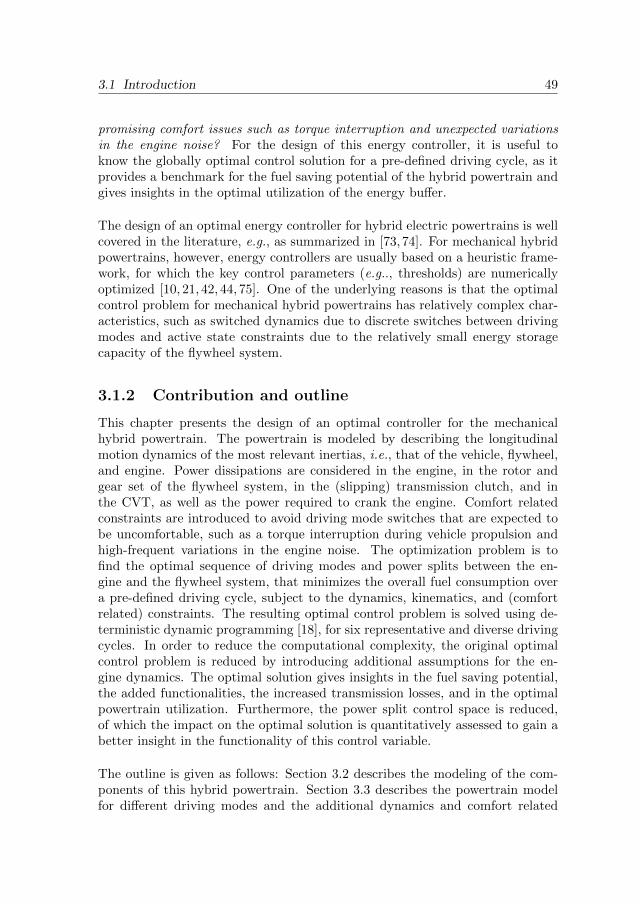
3.1 Introduction 49
promising comfort issues such as torque interruption and unexpected variationsin the engine noise? For the design of this energy controller, it is useful toknow the globally optimal control solution for a pre-defined driving cycle, as itprovides a benchmark for the fuel saving potential of the hybrid powertrain andgives insights in the optimal utilization of the energy buffer.
The design of an optimal energy controller for hybrid electric powertrains is wellcovered in the literature, e.g., as summarized in [73,74]. For mechanical hybridpowertrains, however, energy controllers are usually based on a heuristic frame-work, for which the key control parameters (e.g.., thresholds) are numericallyoptimized [10, 21, 42, 44, 75]. One of the underlying reasons is that the optimalcontrol problem for mechanical hybrid powertrains has relatively complex char-acteristics, such as switched dynamics due to discrete switches between drivingmodes and active state constraints due to the relatively small energy storagecapacity of the flywheel system.
3.1.2 Contribution and outline
This chapter presents the design of an optimal controller for the mechanicalhybrid powertrain. The powertrain is modeled by describing the longitudinalmotion dynamics of the most relevant inertias, i.e., that of the vehicle, flywheel,and engine. Power dissipations are considered in the engine, in the rotor andgear set of the flywheel system, in the (slipping) transmission clutch, and inthe CVT, as well as the power required to crank the engine. Comfort relatedconstraints are introduced to avoid driving mode switches that are expected tobe uncomfortable, such as a torque interruption during vehicle propulsion andhigh-frequent variations in the engine noise. The optimization problem is tofind the optimal sequence of driving modes and power splits between the en-gine and the flywheel system, that minimizes the overall fuel consumption overa pre-defined driving cycle, subject to the dynamics, kinematics, and (comfortrelated) constraints. The resulting optimal control problem is solved using de-terministic dynamic programming [18], for six representative and diverse drivingcycles. In order to reduce the computational complexity, the original optimalcontrol problem is reduced by introducing additional assumptions for the en-gine dynamics. The optimal solution gives insights in the fuel saving potential,the added functionalities, the increased transmission losses, and in the optimalpowertrain utilization. Furthermore, the power split control space is reduced,of which the impact on the optimal solution is quantitatively assessed to gain abetter insight in the functionality of this control variable.
The outline is given as follows: Section 3.2 describes the modeling of the com-ponents of this hybrid powertrain. Section 3.3 describes the powertrain modelfor different driving modes and the additional dynamics and comfort related

50 Chapter 3. Optimal energy control with comfort related constraints
constraints for switches in between. Section 3.4 defines the optimization prob-lem and introduces two reduced optimization problems which are solved withdynamic programming. Section 3.5 presents the simulation results and analyzesthe optimal energy controller designs and their results. Finally, the conclusionsare drawn in Section 3.6.
3.2 Component models
The main components of the hybrid powertrain are the internal combustion en-gine, flywheel system, clutches, CVT, and vehicle. This section describes themodeling of these components, for which some characteristics are summarizedin Table 3.1. The component models describe the longitudinal dynamics (implic-itly) as a function of the vehicle velocity and acceleration, which are prescribedby the driving cycle. The dynamics are described with a forward Euler schemewith a fixed discrete time step of ∆t = 1 s, using a time index “k”. Dynamiceffects acting on a small time scale (i.e., < 1 s) are assumed to be perfectlycontrolled by the component controllers and are not considered. Gear ratiosare defined as the output speed (vehicle side) divided by the input speed (fly-wheel side). The efficiency models are based on static experiments performedunder warm operating conditions, for which some characteristics are shown inChapter 2. The semi-empirical modeling of the power dissipation in the flywheelsystem and CVT are described in detail in Appendix A. For the sake of sim-plicity, only the most relevant (largest) inertias are considered, which are theinertias of the flywheel, engine, and the vehicle. Smaller inertias, such as thatof clutches, gears, and the pulleys of the CVT, are expected to have a negligibleeffect on the fuel consumption. Since the inertia of the gear set is not considered,the flywheel clutch (Ct) may also be modeled after the gear set, resulting in theschematic dynamic model as shown in Fig. 3.2.
3.2.1 Engine
The engine is modeled as an inertia Je on which two torques are acting. Thethermal combustion torque including the frictional torque caused by the movingparts is denoted by τh. The external torque that is used for propulsion is denotedby τe. The resulting engine speed dynamics and the related constraints are givenby

3.2 Component models 51
engine
flywheel system
ωe
τv+τb ωf
ωw Ce
Cf
Ct
ωp τh
τr rg
rv rd
Jr
Je
Jv
CVT τf
τe
τp τw
vehicle clutches
τg
τt
ωs
τs
+
Fig. 3.2. Dynamic model of the mechanical hybrid powertrain (compli-ances are omitted).
Table 3.1. Base component characteristics
engine 4-cylinder 1.5-l gasoline internal combustion engine, powerrange 0−76 kW, rotational speed range 0−630 rad/s, torquerange −17− 140 Nm, mechanical efficiency1 0− 36%
flywheelsystem
vacuum-placed steel rotor, energy storage capacity 150 kJ,power range −25 − 35 kW, rotational speed range 0 −3140 rad/s, torque range −100−140 Nm, gear set transmissionefficiency range1,2 80%−98% rotor power dissipation range1,2
70 − 230 W, inertia 0.03 kgm2, gear set ratio 0.0813, systemmass 27 kg
transmission pushbelt-driven continuously variable transmission, torquerange −100 − 140 Nm, speed ratio range 0.410 − 2.32, finaldrive ratio 0.186, transmission efficiency range1,2 50%− 91%
vehicle Smart ForFour (2005), mass including 2 passengers 1120 kg,combined inertia of the wheels 1.2 kgm, aerodynamic dragcoefficient 0.31, frontal area 1.86 m2, static rolling resistance143 N
1Efficiency characteristic is shown in Chapter 2. 2Semi-empirical modeling isdescribed in Appendix A.

52 Chapter 3. Optimal energy control with comfort related constraints
ωe(k + 1) = ωe(k) +1
Je(τh(k)− τe(k))∆t, (3.1)
ωe ∈
0 if φ = 1,
ωidle else if τe = 0 ∧ vv = 0,
[ωe, ωe] else.
(3.2)
τh ∈ [τh(ωe), τh(ωe)]. (3.3)
The engine has three operation modes, which is reflected in the operating rangefor the engine speed. The engine is shut-off (ωe = 0) in the flywheel drivingmode, which is denoted by φ = 1 and further explained in Section 3.3.1. Theengine is idling at a constant speed (ωe = ωidle) when the vehicle is standing stillwithout generating torque, where vv denotes the vehicle velocity. The enginecan generate a propulsion torque for at higher speeds (ωe ∈ [ωe, ωe]), whereωe > ωidle. The speed-dependent torque range ([τh(ωe), τh(ωe)]) is a function ofthe engine speed, where the lower bound describes the drag torque and the upperbound the wide-open throttle torque. The torque range is described by a look-uptable, for which intermediate values are approximated by linear interpolation.The effective mechanical power Pe follows as
Pe = ωeτe. (3.4)
The associated fuel consumption, in terms of power (or, chemical energy flux)Pf , is described as a function of the speed and torque with a look-up table by
Pf = Pf(ωe, τh). (3.5)
3.2.2 Flywheel system
The flywheel system is modeled as an inertia Jr, on which three torques areacting. The rotor torque τr describes the torque losses caused by aerodynamicdrag and friction in the bearings and seals as a function of the speed. The geartorque τg describes the transmission losses in the gear set as a function of thespeed and transmitted torque, and is modeled at the output shaft. The gear setgives a constant speed ratio rg between the output shaft ωf and the rotor, tooperate the rotor at relatively high rotational speeds (up to 3140 rad/s). Thespeed range of the flywheel system is selected, for its purpose of urban driving,to match the engine speed range (up to 265 rad/s) under normal urban drivingconditions to facilitate a combined operation (i.e., hybrid driving mode). Theexternal torque that is used for propulsion or braking is denoted by τf . Theresulting flywheel speed dynamics and the related constraints are given by

3.2 Component models 53
ωf(k + 1) = ωf(k)− 1
Jr
(r2g(τf(k) + τg(τf(k), ωf(k)))− rgτr(ωf(k))
)∆t. (3.6)
ωf ∈ [0, ωf ], (3.7)
τf ∈ [τ f , τ f ], (3.8)
The kinetic energy content of the rotor Er is given by
Er =Jr
2r2g
ω2f . (3.9)
The power dissipation in the rotor and gear set are given by, respectively,
Pr =τrωf
rg, (3.10)
Pg =τgωf
rg. (3.11)
3.2.3 CVT
The CVT gives a continuously variable speed ratio rv between the primary (sub-script “p”) and secondary pulley shaft (subscript “s”), within fixed geometricalboundaries. The integrated final drive gives a constant speed ratio rd betweenthe secondary pulley shaft and the wheel shaft (subscript “w”). Since no inertiasare considered for the pulleys (or other components), the speeds ω and torque τare related by
ωp =ωw
rvrd, (3.12)
τp = rvrdτw + τt(ωw, τw, rv), (3.13)
where τt(ωw, τw, rv) denotes the torque loss in the transmission modeled at theprimary shaft, and includes the torque loss in the pump, variator, and final drive.The constraints on the speed ratio (rv) and the primary torque (τp) are givenby, respectively,
rv ∈ [rv, rv], (3.14)
τp ∈ [τp, τp]. (3.15)
Constraints on the primary speed are already implicitly given by the constraintson the engine speed (3.2) and on the flywheel system (3.7). The shift rate rv(k)−

54 Chapter 3. Optimal energy control with comfort related constraints
rv(k−1) is not constrained to limit the number of states required to describe thepowertrain model. It is assumed that the CVT does not require higher shift ratesto accelerate or decelerate the flywheel system than conventionally necessary forthe engine, because of the relatively high inertia of the flywheel system. Therequired clamping forces, however, may be higher and may limit the shift rate,but this effect is not considered here. The power dissipation in the CVT is givenby
Pt = τtωp. (3.16)
3.2.4 Clutches
The hybrid powertrain contains three actively controlled clutches, which are theengine clutch (subscript “e”), flywheel clutch (subscript “f”), and transmissionclutch (subscript “t”). The compact engine clutch and flywheel clutch are onlysuitable to synchronize the intermediate shaft between the clutches and to crankthe engine, sufficient to select different driving modes of the powertrain, as will bedescribed in Section 3.3.1. It is assumed that these clutches engage, or disengagewithin one time step (i.e., 1 s). Then, the clutches can be modeled by twodiscrete states
Ci : =
0, ⇐⇒ disengaged1, ⇐⇒ engaged
, i ∈ e, f. (3.17)
The transmission clutch has conventional dimensions and will only be used toaccelerate the vehicle (or, flywheel) from standstill, which may take several timesteps (i.e., > 1 s). When slipping, the transmitted clutch torque τp is controlledby a hydraulic actuator that manipulates the pressure force on the clutch plates.The torque can only be transmitted from the high-speed side to the low-speedside of the clutch, so
sign(τp) = sign(ωc), (3.18)
ωc =
ωe − ωp, if Ce = 1,
ωf − ωp, if Cf = 1,(3.19)
where ωc denotes the slip speed. The associated power dissipation is modeledby
Pc = τpωc. (3.20)

3.2 Component models 55
The overall power dissipation is kept low by choosing a speed ratio for the CVTthat minimizes the slip speed, i.e., rv = rv when accelerating the vehicle fromstandstill. The transmission clutch engages as soon as the velocity of the vehiclesynchronizes with the rotational speed of the engaged power source, i.e., theflywheel system, and/or the engine. When engaged (i.e., ωc = 0), the clutch cantransmit torque in either direction with virtually no power dissipation.
3.2.5 Vehicle
The vehicle model describes the wheel shaft speed ωw and the required power-train torque τw to track the prescribed vehicle velocity vv and vehicle accelerationav of the driving cycle. Assuming no wheel slip, the dynamic wheel radius Rw
gives a constant speed ratio between the vehicle velocity and the wheel shaftspeed. The mass of the vehicle, two passengers of 75 kg, and the inertias of thewheels are lumped into an equivalent inertia Jv at the wheel shaft, on whichthree torques are acting. The drag torque τv describes the combined rolling andaerodynamic resistance as a function of the vehicle velocity vv. The brakingtorque τb describes the friction torque of the disc brakes, whereas τw describesthe propulsion or braking torque provided by the powertrain torque. The modelsare given by
ωw =vv
Rw, (3.21)
τw =Jv
Rwav + τv(vv)− τb. (3.22)
Ideally, all available brake energy is recuperated by the flywheel system, soτb = 0, but this is not always possible as the flywheel system can only brakethe front wheels, which may lead to vehicle instability at high decelerations. Formedium decelerations up to av > −4 m/s2s (the maximum deceleration seenin most driving cycles), the front wheels may apply 94% of the brake torquewithin European safety regulations [76, 77]. Another requirement to maximizebrake energy recuperation is the use of a certified brake-blend (or, brake-assist)system, which safely intervenes between the brake pedal and the disc brakesto provide the desired torque-split for braking [70]. In this study, in order tokeep the cost of the flywheel system potentially low, the use of such a system iscircumvented by a parallel braking strategy1, where the flywheel system brakesin parallel to the disc brakes. As a consequence, the driver may notice a higherbrake pedal sensitivity (pedal force to vehicle deceleration), yet this is expectedto be acceptable since large variations in brake pedal sensitivity are observedbetween different vehicles, e.g., up to a factor 9 for low decelerations in [78].Possibly interesting implementations are to apply a regenerative braking that
1The effects on the Anti-lock Braking System need further investigation.

56 Chapter 3. Optimal energy control with comfort related constraints
approximates the engine drag torque, or to use a part of the “dead stroke”of the brake pedal, i.e., to start with regenerative braking when the pedal isslightly pressed while the disc brakes are not yet actuated. A drawback of theparallel braking strategy, however, is the unavoidable inconsistency in brakepedal response when the flywheel system reaches its energy storage limit, orwhen switching between driving modes, so an acceptable trade-off must be foundbetween brake energy recuperation and brake pedal response. It is assumed thatthis trade-off can be found with an average relative brake power split β, so that
τb = β
(Jv
Rwav + τv(vv)
), (3.23)
β =
0 if ( JvRw
av + τv(vv)) ≥ 0,
0.33 else if ωf < ωf ,
1 else.
(3.24)
The power dissipations by the disc brakes and by the vehicle (aerodynamic androlling resistance) are given by, respectively,
Pb = τbωw, (3.25)
Pv = τvωw, (3.26)
3.3 Powertrain model
The hybrid powertrain can be operated in several driving modes, which can bedescribed by the states of the engine clutch and flywheel clutch. This sectionexplains each relevant driving mode and the additional dynamics and constraintsfor the switching between driving modes.
3.3.1 Driving modes
The hybrid powertrain can be operation in three relevant driving modes, wherethe engine and flywheel clutch are either disengaged or engaged. The drivingmodes φ are defined by
φ :=
1 ⇐⇒ Ce = 0, Cf = 1,2 ⇐⇒ Ce = 1, Cf = 1,3 ⇐⇒ Ce = 1, Cf = 0.
(3.27)
According to this definition, the driving mode decides which power source is usedto propel the vehicle: either the flywheel system (φ = 1), the engine (φ = 3), or

3.3 Powertrain model 57
Table 3.2. Powertrain operation during various driving modes.
φ description τe τf rv
1 flywheel driving 0 τp ωs/ωf
2 hybrid driving τp − τf τp − τe + τcrank ωs/ωf
3 engine driving τp τcrank ωs/ωe
Constraints apply, cf. (3.2), (3.3), (3.7), (3.8), (3.14), (3.15), (3.18).
both (φ = 2). Notice that the driving mode does not depend on the transmissionclutch state Ct, as this clutch is only used to accelerate the vehicle (or, flywheel)from standstill, and not to switch between power sources. Each driving mode isexplained in more detail below:
• In the flywheel driving mode (φ = 1), the flywheel system is used to propelor brake the vehicle while the engine is disengaged and shut-off. Withinthis mode, fuel consumption is reduced by brake energy recuperation forlater use, and by shutting off the engine. The speed ratio of the CVT (rv)follows implicitly from the powertrain dynamics and the prescribed drivingcycle.
• In the hybrid driving mode (φ = 2), the engine propels the vehicle whilesimultaneously, the flywheel system is energized (τf < 0), or de-energized(τf > 0) to assist the engine. The power split can be determined bythe engine torque τe, or by the relative power split σ as defined later inSection 3.4.2. Within this mode, inefficient part-load operation of theengine is eliminated by energizing the flywheel system while propelling thevehicle.
• In the engine driving mode (φ = 3), the engine propels the vehicle whilethe flywheel system is disengaged and coasting. The operation point of theengine can be determined by the engine torque τe, or by the speed ratio rv.Within this mode, the vehicle is propelled with conventional performance,but without reduction of the fuel consumption.
The required propulsion torque(s) from the power source(s), as well as the cor-responding speed ratio of the CVT, are summarized for each driving mode inTable 3.2. For some driving mode switches, an additional torque is required de-noted by τcrank, as will be derived in the sequel, and equals zero when no switchtakes place.
3.3.2 Switching between driving modes
There are six different switches possible between the three driving modes. Thedriving mode switches can be uniquely identified by considering the previous

58 Chapter 3. Optimal energy control with comfort related constraints
Table 3.3. Switches between driving modes.
φpre φ dynamics and constraints
1 2 engine cranking (3.28), high-frequent switching (3.32)1 3 engine cranking (3.28), clutch disengagement2 1 clutch disengagement2 3 clutch disengagement, engine synchronization3 1 torque interruption (3.30), (3.31), clutch disengagement3 2 torque interruption (3.30), (3.31), high-frequent switching (3.32)
driving mode φpre(k) = φ(k − 1) as a powertrain state. Each driving modeswitch is characterized by different powertrain dynamics, of which some mustbe constrained in order to guarantee a fast and smooth powertrain response,with an acceptable consistency of the engine noise. The associated dynamicsand constraints are listed in Table 3.3 and explained in more detail below.
3.3.2.1 Clutch disengagement and engine synchronization
When disengaging the engine clutch or the flywheel clutch, it is assumed thatno additional drag torques are introduced and no power is dissipated. Afterdisengagement of the flywheel clutch, a significant engine torque may be requiredto change the engine speed cf. its dynamics in (3.1).
3.3.2.2 Engine cranking
The engine is cranked with the flywheel system by smooth engagement of theengine clutch. It is assumed that the clutch engagement is sufficiently smoothsuch that driver does not feel it. The torque τcrank to crank the engine fromωe(k − 1) = 0 to ωe(k) = ωf(k) through a slipping engine clutch is modeled by
τcrank(k) =
Je
ωe(k)−ωe(k−1)∆t + τh(ωe(k)) if φ(k) 6= 1 ∧ φpre(k) = 1,
0 else.(3.28)
The associated power is given by
Pcrank = τcrankωf . (3.29)
3.3.2.3 Torque interruption
Fast and smooth engagement of the flywheel clutch is only possible when notorque is transmitted (i.e., τw = 0), since the clutch is not designed to dissipate

3.3 Powertrain model 59
high powers. This would imply an uncomfortable torque interruption duringvehicle propulsion, which can only be avoided by
φ = 3 if φpre = 3 ∧ τw > 0 (3.30)
During vehicle braking, however, the situation is different, since the disc brakesprovide the braking torque. The transmission clutch can be disengaged as soonas the brake pedal is pressed, after which the flywheel clutch can be engagedto synchronize the intermediate shaft with the flywheel system, while the (un-loaded) CVT can quickly shift to the desired speed ratio if necessary. After that,the transmission clutch can be used for a smooth clutch engagement, thereby al-lowing brake energy recuperation after engine driving. This switch may requirea smoothly changing brake power split for an acceptable brake pedal response.
To guarantee a fast torque generation of the engine, e.g., to handle change-of-mind actions of the driver, a minimum engine speed ωe is required cf. 3.3.This implies a minimum flywheel speed for the engine cranking, but also for thehybrid driving mode, due to the mechanical connection between the engine andflywheel system. This comfort related constraint is approximated, i.e., withoutconsidering the small reduction in the flywheel speed while cranking the engine,by
φ = 3 if ωf < ωe. (3.31)
When ωf < ωe, an exception is made for the engine mode definition as describedby (3.27) and in Table 3.3, by allowing brake energy recuperation to energizethe flywheel system, while the engine is idling.
3.3.2.4 High-frequent switching
The engine noise frequency rises when the flywheel is energized during hybriddriving, which may be counterintuitive to the driver under certain driving con-ditions. Therefore, for an acceptable consistency of the engine noise, hybriddriving is avoided when no propulsion torque is required (i.e., τw ≤ 0) to keepthe noise level low, and outside urban areas (i.e., vv > vu) to limit engine noisevariations that result from duty-cycle switching between hybrid and flywheeldriving. Here, vu denotes an arbitrary velocity threshold, which is chosen asthe maximum urban velocity in The Netherlands of 13.9 m/s (50 km/h). Thehigh-frequent switching is already penalized with a soft constraint by taking thepower to crank the engine into account cf. (3.28), whereas a hard constraint isintroduced by
φ ∈ 1, 3 if τw ≤ 0 ∨ (φpre 6= 2 ∧ vv > vu). (3.32)

60 Chapter 3. Optimal energy control with comfort related constraints
The flywheel driving mode is not constrained to avoid limitations on the utiliza-tion of recuperated brake energy.
3.3.3 Driving cycles
The optimal controller for this hybrid powertrain is computed for six represen-tative driving cycles, which are the Japan Cycle 08 (JC08), the New EuropeanDriving Cycle (NEDC), the Federal Test Procedure ’75 (FTP75), the “low”,“medium”, and “high” parts of the Worldwide harmonized Light vehicles TestProcedure (WLTP), the “urban” part of the Common Artemis Driving Cycle(CADC), and the sportive Eindhoven driving cycle (EHV), as shown in Fig. 3.3.The JC08, NEDC, and FTP75 are selected to represent certified driving cy-cles in the most important continents of the automotive industry, i.e., Asia,Europe, and North-America, whereas the WLTP, CADC, and EHV representreal-world driving behavior measured in, respectively, worldwide industrializedcountries [79], Europe [80], and Eindhoven (The Netherlands). Since the fly-wheel system is aimed for urban use, highway cycles such as the “extra high”part of the WLTP and the “extra urban” and “highway” parts of the CADCare not considered. All of the driving cycles have, as the majority of the drivingcycles found in the literature, no variations in altitude, wind, or road surface.The diversity of the driving cycles will be shown next, by introducing three char-acterizing indices that are directly related to the fuel saving functionalities.
The average absolute acceleration quantifies the variations in kinetic energy ofthe vehicle, which can be related to the effectiveness of brake energy recupera-tion. The average absolute acceleration av is defined for the non-standstill partsof the driving cycle with time range [k0, kn] by
av :=
∑knk=k0
n(k)|av(k)|∆t∑knk=k0
n(k), (3.33)
n(k) :=
0 if vv(k) = 0 ∧ av(k) = 0,
1 else,(3.34)
where n(k) can be considered as a conditional sampler. The average absolutevelocity quantifies the mix of urban and extra urban driving, which can berelated to the fuel saving potential of the flywheel system that is aimed forurban driving. The average absolute velocity vv is defined for the non-standstillparts of the driving cycle, and is given by
vv :=
∑knk=k0
n(k)|vv(k)|∆t∑knk=1 n(k)
. (3.35)

3.3 Powertrain model 61
v v[m
/s]
0 200 400 600 800 10000
10
20
30 NEDC
v v[m
/s]
0 500 1000 15000
10
20
30 FTP75
v v[m
/s]
0 200 400 600 800 1000 1200 14000
10
20
30 WLTP
v v[m
/s]
0 100 200 300 400 500 600 700 8000
10
20
30 EHV
v v[m
/s]
0 200 400 600 800 1000 12000
10
20
30 JC08
v v[m
/s]
time [s]
0 200 400 600 8000
10
20
30 CADC
Fig. 3.3. Representative and diverse selection of certified and real-worlddriving cycles.
The relative standstill time quantifies the idling time (or, standby time) of thevehicle, e.g., due to traffic lights, or traffic congestion, which can be related tothe idling losses of the engine. The relative idling time (tidle) is defined by
tidle := 1−kn∑k=k0
n(k)t(k)∆t. (3.36)
The three indices av, vv, and tidle are shown for the six driving cycles in Fig. 3.4,

62 Chapter 3. Optimal energy control with comfort related constraints
av/a
v[%
]
0
10
20
30v v
/vv
[%]
0
10
20
30
40
t idle/t
v(k
n)
[%]
NEDC JC08 WLTP FTP75 CADC EHV0
10
20
30
Fig. 3.4. Driving cycle characteristics related to the hybrid powertrainfunctionalities for the selected driving cycles.
with respect to the maximum acceleration av and the maximum velocity vv of alldriving cycles, and with respect to the driving cycle length tv(kn), respectively.From av, it follows that the certified driving cycles (NEDC, JC08, and FTP75)are relatively mild, whereas the real-world driving cycles (CADC and EHV) arerelatively sportive, except for the WLTP. From vv, ar clear distinction is observedbetween the mixed driving cycles (NEDC, FTP75, and WLTP) and the urbandriving cycles (JC08, EHV, and CADC). From tidle, large differences are observedamong the driving cycles. Overall, it can be concluded that the selected drivingcycles represent a diverse mix with different fuel saving possibilities.
3.4 Optimization
In order to find the optimal controller, it is convenient to write the powertraindynamics as a function of the states, control variables, and external states. For aprescribed driving cycle, the hybrid powertrain dynamics can be controlled withtwo control variables, which are the driving mode (φ) and the engine torque (τe).Note that the engine torque disappears as a control variable when the engine isshut-off, i.e., in the flywheel driving mode. The associated control vector u isdefined as

3.4 Optimization 63
u := [φ, τe]T. (3.37)
The hybrid powertrain dynamics can be described with three system states,which are related to the flywheel system dynamics (3.6), the driving mode dy-namics (see, Section 3.3.2), and the engine speed dynamics (3.1). The followingstates are selected: the kinetic flywheel energy content Er (ωf is also suitable),the previous driving mode φpre, and the engine speed ωe. The associated statevector x is defined as
x := [Er, φpre, ωe]T. (3.38)
The prescribed driving cycle can be written as an external state vector w, whichcontains the vehicle velocity (vv) and acceleration (av), i.e.,
w := [vv, av]T. (3.39)
Using the definitions (3.37)-(3.39), the powertrain dynamics and kinematicsgiven by (3.1), (3.6), (3.9), (3.12), (3.13), (3.17), (3.19), (3.21), (3.22), (3.23),(3.24), (3.27), (3.28) can be compactly written as
x(k + 1) = x(k) + f(x(k), u(k), w(k))∆t. (3.40)
3.4.1 Problem formulation
The main objective of the controller is to minimize the overall fuel consumptionfor a prescribed driving cycle with time range [k0, kn], i.e.,
minu(k)
kn−1∑k=k0
Pf(x(k), u(k), w(k))∆t, (3.41)
subject to
• the powertrain kinematics and dynamics given by (3.40);
• the physical operating limits given by (3.2), (3.3), (3.7), (3.8), (3.14),(3.15), and (3.18); and
• the comfort related constraints given by (3.31), (3.30), and (3.32).

64 Chapter 3. Optimal energy control with comfort related constraints
There is no final (energy) state constraint for energy sustenance as often seen forhybrid electric powertrains [73], since the flywheel system can only store energyfor a relatively short term (< 30 min.). Nevertheless, the final energy level isusually non-zero due to brake energy recuperation at the end of the drivingcycle. The start conditions at time index k = k0 represent “warm” conditions,where the powertrain is already at operating temperature, the flywheel systemcontains 50% of its energy storage capacity (Er(k0) = 0.5Er = 75 kJ), and thepowertrain starts in the flywheel driving mode (φ(k0) = 1). The signal flowof this optimization problem is schematically depicted in Fig. 3.1, showing thecontrol variables φ (i.e., clutch states Ce and Cf) and τe, the external states vv
and av, and the optimized variable Pf .
3.4.2 Problem reductions
The optimal control problem is characterized by
• switched dynamics due to discrete driving modes;
• active state constraints, due to the relatively small energy storage capacityof the flywheel system and the mechanical connection between the engineand the flywheel system; and
• non-convex control constraints to avoid uncomfortable driving mode switches.
This class of optimization problems is relatively difficult to solve analytically, butcan be solved numerically using deterministic dynamic programming [18]. Thenumerical optimization of two control variables in a 4-dimensional time-statespace, however, requires a relatively long computation time. Therefore, in orderto reduce the computational complexity, additional assumptions are introducedfor the engine driving mode and the hybrid driving mode. Besides computationalbenefits, reducing the optimal control problem may also contribute to a betterunderstanding of the controlled system.
3.4.2.1 Reduced engine model
During engine driving (φ = 3), it is assumed that the optimal engine speedchanges very slowly, so that ωe(k + 1) ≈ ωe(k), and implicitly, τh ≈ τe holds.The remainder of the powertrain can still be in transient condition as the vehicletracks the prescribed velocity profile given by the driving cycle. This assumptionis often found in the literature and seems reasonable with fuel-optimal operationof the engine [81–83]. Based on this assumption, the optimization problemcan be reduced by eliminating state x3 (i.e., ωe), whereas the engine dynamicsdescribed by (3.1) can be reduced to the kinetic relation

3.4 Optimization 65
ωe =τwωw
τe − τt, (3.42)
By eliminating these dynamics, the control variable u2 can be eliminated forφ = 3, as the engine operation point can now be optimized statically by
τe = arg minτe
Pf(φ = 3). (3.43)
When switching between driving modes, however, accelerations in the enginespeed may be significant. These accelerations can still be considered cf. (3.1)without x3, by reconstructing the accelerations using the previous driving modestate (φpre), and the relations ωe = 0 for φ = 1, ωe = ωf for φ = 2, and (3.42)for φ = 3.
3.4.2.2 Reduced power split control space
During hybrid driving mode (φ = 2), the engine operating point can be conve-niently described by the relative power split σ, which is defined as the torquereserve fraction of the engine that is used to energize the flywheel system, by
σ :=τh − τpτh − τp
. (3.44)
So, σ < 0 implies boosting of the engine using the flywheel, σ = 0 impliesengine driving while the flywheel remains engaged, which can be interpretedas the hybrid variant of engine driving, and σ = 1 implies maximal flywheelenergizing. It is assumed that the main functionality of the hybrid drivingmode is the efficient energizing of the flywheel system. However, due to thecomfort related constraint with engine driving (3.30), which restricts drivingmode switches during vehicle propulsion, there is also a second functionality, i.e.,to maintain the control flexibility while propelling the vehicle using solely theengine. Based on this assumption, the control space of u2 can be substantiallyreduced for φ = 2 to only two values:
σ ∈ 0, σ∗, (3.45)
where the energizing power split σ∗ is statically optimized by
σ∗ := arg minσ
Pf(σ, φ = 2)
Pe(σ, φ = 2). (3.46)
The impact of this control space reduction on the solution is quantitativelyassessed in the sequel.

66 Chapter 3. Optimal energy control with comfort related constraints
Table 3.4. Simulation settings.
# powertrain power split optimization φ(k) σ(k)
1 conventional - 3 -2 hybrid full ∈ 1, 2, 3 ∈ [0, 1]3 hybrid reduced ∈ 1, 2, 3 ∈ 0, σ∗
3.4.3 Dynamic programming
The optimization problem given by (3.41) is solved for the six driving cycles,using several simulation settings to investigate the performance of the mechan-ical hybrid powertrain compared to its conventional (non-hybrid) counterpart.For the conventional powertrain, the same powertrain model is used, except forthe flywheel system mass of 27 kg, the flywheel system dynamics (i.e., no brakeenergy recuperation), and a restricted control variable φ(k) = 3. Furthermore,the impact of reducing the control space using (3.45) and (3.46) on the solutionis investigated. The resulting simulation settings are listed in Table 3.4. For allsimulation settings, the engine model is reduced by (3.42) and (3.43).
Deterministic dynamic programming is used to find the globally optimal solution,in the sense of achievable optimality despite approximation errors introduced bymathematical modeling and numerical quantization. The continuous optimalcontrol problem is implemented in the discrete framework using a computation-ally efficient implementation method that avoids nearest-neighbor rounding ofthe state trajectories, as described in Appendix B. In this discrete framework,the continuous energy state (Er) is quantized into 150 evenly distributed values,whereas the continuous (non-reduced) relative power split (σ) is quantized into20 evenly distributed values in [0, 1]. Boosting of the engine (i.e., σ < 0) is notconsidered, since it does not contribute to a lower overall fuel consumption.
3.5 Results and discussion
The optimization results are compared to answer the following research ques-tions: i) what is the fuel saving potential of the mechanical hybrid powertrain,ii) what is the impact of the control space reduction on the fuel saving potential,and iii) how is the hybrid powertrain optimally controlled?
3.5.1 Fuel saving potential
The top graph of Fig. 3.5 shows the fuel saving potential of the hybrid power-train with respect to the conventional powertrain for each of the driving modes.It can be seen that, despite the relatively low energy storage capacity of the

3.5 Results and discussion 67
flywheel system, a fuel saving can be achieved between 20.2% and 40.6%, whichdepends on the selected driving cycle. As expected, since the flywheel systemis aimed for urban use, a lower fuel saving is achieved with driving cycles thatcontain extra-urban or highway parts, such as the NEDC, WLTP, and FTP75(see, Fig. 3.4). Note that this trend holds for hybrid vehicles in general. Thehighest fuel saving is obtained for the CADC, due to the sportive and urbandriving characteristics with a relatively long idling time (see, Fig.3.4). Recallthat with these computations the disc brakes are assumed to absorb 33% of thebraking energy cf. (3.24), to avoid the use of a brake-blend system. Simula-tions with minimal use of the disc brakes, i.e., only limited by vehicle stabilityrequirement (β = 0.06), gives a slightly better (1%− 5%) fuel saving potential,but it is expected that it does not justify the additional cost of a brake-blendsystem.
ΔE
f/E
conv
f[%
]
−40
−30
−20
−10
0
hybridization (#2 w.r.t. #1)
ΔE
f/E
conv
f[%
]
NEDC WLTP FTP75 EHV JC08 CADC0
0.1
0.2
0.3
0.4 problem reduction (#3 w.r.t. #2)
Fig. 3.5. The fuel saving potential of the hybrid powertrain with respectto the conventional powertrain (top graph) and the impact of reducingthe power split control space on the fuel saving potential (bottom graph).The fuel saving potential is computed as the difference in the overall fuelconsumption (∆Ef) with respect to the overall fuel consumption of theconventional powertrain (Econv
f ).
The bottom graph of Fig. 3.5 shows the impact of the reduced optimizationproblem with respect to the full optimization problem. It is observed that thereduced optimization problem gives a sub-optimal result, yet the optimizationerror is negligible (0.2% − 0.4%). This result confirms that the hybrid drivingmode only serves two functionalities, which are i) efficient energizing of the

68 Chapter 3. Optimal energy control with comfort related constraints
flywheel system, and ii) “engine driving” while maintaining control flexibility.
3.5.2 Energy controller
Detailed results of the energy controller and the associated powertrain dynamicsare shown for the three simulation settings and the very different NEDC andEHV in, respectively, Figs. 3.6 and 3.7. The relatively static NEDC containsmany constant-velocity parts, low accelerations, and a highway part, whereasthe relatively dynamic EHV contains many sportive accelerations and deceler-ations and no highway part. From top to bottom, the seven graphs depict,respectively, the velocity of the vehicle (vv), the driving mode (φ) together withthe relative power split (σ), the kinetic energy content of the rotor (Er), theCVT speed ratio (rv), the engine speed (ωe), the engine torque (τe), and thecumulative fuel consumption in terms of energy (Ef). It can be seen that thefuel saving functionalities are generally used as follows: at standstill, the engineis shut-off while the flywheel system is coasting (φ = 1). At low vehicle ve-locities and low accelerations, the flywheel system accelerates the vehicle fromstandstill and propels the vehicle accordingly (φ = 1). At low velocities andmedium accelerations, the flywheel system cranks the engine and the enginepropels the vehicle while energizing the flywheel system (φ = 2). At high veloc-ities and/or high acceleration, the engine propels the vehicle and the flywheelsystem is disengaged (φ = 3). Overall, the flywheel system is energized withbrake energy (φ = 1) when possible, and using the engine (φ = 2) otherwise.In the hybrid driving mode, roughly two power split (σ) values are observed forthe full optimization problem, which correspond to those of the reduced opti-mization problem. Often, the power split is increased shortly before switchingto the flywheel mode (φ = 1), so that the buffered energy can be immediatelyused, having limited storage losses.
Overall, the flywheel speed (related to Er) and the engine speed (ωe) are keptrelatively low to limit the power dissipation in the engine, rotor, gear set, driveclutch, and CVT. The engine is operated at fuel-efficient high torques (τe), exceptfor some parts in the NEDC (between 850 s and 1100 s), which can be explainedby the comfort related constraints (3.30) and (3.32). The speed ratio of the CVT(rv) is quite similar for the conventional powertrain and the hybrid powertrain,due to the similar speed range of the both engine and the flywheel system.Small differences can be observed in the control variables (φ and σ) betweenthe solutions of the full and reduced optimal control problems, which are alsoreflected in the energy state (Er). However, despite local deviations, the overalldifference is very small, resulting in a negligible difference in the overall fuelconsumption (Ef). These results suggest that for some parts in the drivingcycle, various state trajectories exist that result in nearly the same overall fuelconsumption.

3.5 Results and discussion 69
v v[m
/s]
0
20φ,σ
[-]
0
1
2
3
Er
[kJ]
0
50
100
150
r v[-]
0.51
1.52
ωe
[rad
/s]
0
100
200
300
τ e[N
m]
0
50
100
Ef
[MJ]
time [s]
0 200 400 600 800 10000
10
20 conventional (#1)
hybrid full (#2)
hybrid reduced (#3)
Fig. 3.6. Energy controller and powertrain dynamics for the NEDC usingthree simulation settings. (Top to bottom) Vehicle velocity (vv), drivingmode (φ) and power split (σ), flywheel energy (Er), CVT speed ratio (rv),engine speed (ωe), engine torque (τe), and cumulative fuel consumption(Ef).

70 Chapter 3. Optimal energy control with comfort related constraints
v v[m
/s]
0
10
20φ,σ
[-]
0
1
2
3
Er
[kJ]
0
50
100
150
r v[-]
0.51
1.52
ωe
[rad
/s]
0
100
200
300
τ e[N
m]
0
50
100
Ef
[MJ]
time [s]
0 100 200 300 400 500 600 700 8000
10
conventional (#1)
hybrid full (#2)
hybrid reduced (#3)
Fig. 3.7. Energy controller and powertrain dynamics for EHV usingthree simulation settings. (Top to bottom) Vehicle velocity (vv), drivingmode (φ) and power split (σ), flywheel energy (Er), CVT speed ratio (rv),engine speed (ωe), engine torque (τe), and cumulative fuel consumption(Ef).

3.5 Results and discussion 71
3.5.3 Fuel saving functionalities
The fuel saving of the hybrid powertrain can be attributed to the added func-tionalities. These functionalities reduce the overall fuel consumption (Ef) byfour effects: the required mechanical energy (Ee) is on one hand reduced due toi) brake energy recuperation, i.e., less brake losses (Eb), but on the other handincreased by ii) higher transmission losses (Et). The required mechanical energyis generated with a higher mechanical efficiency (Ee/Ef(ωe 6= ωidle)) due to iii)the reduced inefficient part-load operation and iv) the elimination of idling losses(Ef(ωe = ωidle)) during vehicle standstill. These effects are related with eachother by
Ef = Ef(ωe = ωidle) +Ef(ωe 6= ωidle)
Ee(Ev + Eb + Et) , (3.47)
where Ev denotes the vehicle losses due to the rolling and aerodynamic resis-tance. The top graph of Fig. 3.8 shows the impact of the change in energy dissi-pation on the fuel saving potential (simulation #2 with respect to #1), where theimpact of the higher transmission losses is indicated by the upward arrow, andthe impact of the three fuel saving functionalities is indicated by the downwardarrow. The average mechanical efficiency is significantly improved due to theelimination of engine idling (4.1%−11.2%), especially for the driving cycles witha relatively long standstill time (see, Fig. 3.4), and due to the reduced part-loadoperation of the engine (13.5% − 20.9%). The generated mechanical energy issignificantly reduced with brake energy recuperation (10.7%− 30.5%), but thiseffect is largely canceled by the increased transmission losses (10.9% − 18.8%),except for the sportive driving cycles due to the relatively many decelerations(see, Fig. 3.4). Overall, it can be concluded that for this mechanical hybrid pow-ertrain, each of the three functionalities contributes significantly to the overallfuel saving: ranging from roughly 5−10% for shutting off the engine during vehi-cle standstill, to ∼ 10−20% for the elimination of inefficient part-load operationof the engine, and 15− 25% for the recuperation of brake energy. Usage of theflywheel system, however, increases the transmission losses, thereby significantlyreducing the fuel saving potential with roughly 10 − 20%, such that 20 − 40%remains.
The bottom graph of Fig. 3.8 gives a more detailed view on the increased trans-mission losses, which is decomposed into the additional energy dissipation inthe rotor, gear set, transmission clutch, CVT, and due to engine cranking. Thehigher losses are partly due to the more frequent utilization of the hybrid trans-mission, i.e., also during regenerative braking, and partly due to the (on average)higher operating speed of the flywheel system. It is observed that the CVT, thecombined transmission clutch and engine cranking, and the combined flywheelgear and flywheel rotor, have each a similar contribution of roughly 4 − 6%.

72 Chapter 3. Optimal energy control with comfort related constraints
ΔE
f/E
conv
f[%
]
−40
−20
0
20
brake energyefficient operationno idling
ΔE
f/E
conv
f[%
]
NEDC WLTP FTP75 EHV JC08 CADC0
5
10
15
20
25 flywheel gearflywheel rotorengine crankingclutchCVT
transmission losses
hybrid functionalities
Fig. 3.8. Results: the effect of each fuel saving functionality on the fuelsaving potential of the hybrid powertrain. The higher transmission lossesincrease the overall fuel consumption, whereas the three functionalities,i.e., i) brake energy recuperation (light gray), ii) reduction of inefficientengine operation (dark gray), and iii) idle-stop of the engine (black), de-crease the overall fuel consumption.
Although the overall increased transmission losses is relatively high, it is notexpected that additional cooling is necessary, since the higher power dissipationmainly occurs during low-power urban driving, while it is well distributed overtime (i.e., propulsion and braking) and among the different components.
Table 3.5 shows the optimal utilization of the hybrid powertrain from a differentperspective. The flywheel system is energized by either recuperated brake energyor by the engine. As can be seen, the relative contribution of each power sourceis on average almost equal, yet large differences are observed between drivingmodes. For example, the flywheel system is mainly energized using the enginefor the mild JC08, and using brake energy for the sportive EHV. Differences arealso observed in the average switching frequency of the driving modes and theengine. As expected, the mild and mixed (urban and highway) driving cycles(NEDC, WLTP, FTP75, and JC08) show relatively low frequencies, as the fly-wheel system is not used on the highway parts, whereas the sportive and urbandriving cycles (EHV and CADC) show relatively high frequencies. Overall, theaverage switching frequency is expected to be acceptable for the driver, providedthat the powertrain response remains quick, smooth, and consistent. For exam-

3.6 Conclusions 73
Table 3.5. Optimal utilization of the hybrid powertrain.
NEDC WLTP FTP75 EHV JC08 CADC
flywheel energizing source [%]:- brake energy 38 49 44 73 36 51- engine energy 62 51 56 27 64 49
average switching frequency [1/min]:- driving mode 2.1 2.4 2.7 4.2 2.6 3.2- engine on/off 1.1 1.3 1.4 2.4 1.4 1.6
ple, the number of driving mode switches on the NEDC (42) is comparable to the(fuel-optimal) number of gear shifts for a stepped transmission (33), as describedin [84]. However, this number may increase when using a real-time controllerthat cannot exploit the exact knowledge about future driving conditions.
3.6 Conclusions
A dynamic model is presented for a mechanical hybrid powertrain, which de-scribes three relevant driving modes and comfort related constraints to avoiduncomfortable driving mode switches. This model is used to find the optimalsequence of driving modes and power splits between the engine and flywheel sys-tem, that minimizes the overall fuel consumption for a pre-defined driving cycle.This relatively complex optimization problem is solved for six representativedriving cycles using dynamic programming. Results show that, despite the rela-tively low energy storage capacity of the flywheel, very high fuel savings can beobtained of between 20%−40%, dependent on the driving cycle. Analysis of theresults shows that each fuel saving functionalities, i) recuperation of brake en-ergy for later use, ii) elimination of inefficient part-load operation of the engine,and iii) engine shut-off during vehicle standstill, contributes with a significantamount to the fuel saving potential, although a part of the fuel saving potentialis canceled by the increased power dissipation in the transmission. The powerdissipation is partly increased due to a more frequent usage, i.e., also duringbrake energy recuperation, and partly due the higher rotational speeds of thetransmission components. Nevertheless, additional cooling is not expected tobe necessary, since the higher power dissipation mainly occurs during low-powerurban driving, while it is well distributed over time and among the differentcomponents. The design problem for the energy controller can be substantiallyreduced by considering only two power split values, instead of a quantized range,with a negligible impact on the fuel saving potential (difference < 0.4%) and the

74 Chapter 3. Optimal energy control with comfort related constraints
optimal energy controller. This result is an important step towards the designof an effective yet simple energy controller that is suitable for implementationin real-time hardware.

Chapter 4
Optimal energy control with coldstart conditions
Abstract – This chapter investigates the impact of cold start conditions on the fuel saving
potential and the associated optimal energy controller of a mechanical hybrid powertrain. The
cold start conditions refer to a low powertrain temperature, which increases the frictional power
dissipation in the engine and transmission, and a stationary (or, energy-less) flywheel system,
which must be energized to a minimum energy level before it can be effectively utilized. The
heating of the powertrain and the initialization of the flywheel system can be influenced by
the energy controller, which controls the power distribution between the engine, flywheel, and
vehicle. The energy controller aims at minimizing the overall fuel consumption for a given
driving cycle. The optimal energy controller is found analytically for a simplified model to
gain qualitative insights in the controller, and numerically using dynamic programming for a
detailed model to quantify the impact on the fuel consumption. The results show that the
cold start conditions have a significant impact (4.3% − 7.6%) on the fuel saving potential, yet
a negligible impact on the optimal energy controller.
4.1 Introduction
Hybrid powertrains improve the fuel economy of passenger vehicles significantlyby adding a secondary power source to the internal combustion engine. Thesecondary power source is able to store energy from the engine and to exchangeenergy with the propelled vehicle. A low-cost alternative to the state-of-the-art hybrid electric powertrains is a mechanical hybrid powertrain, which uses acompact flywheel system for kinetic energy storage and mechanical componentssuch as a Continuously Variable Transmission (CVT) and clutches for powertransmission [8]. The power flows between the engine, flywheel, and vehicle are

76 Chapter 4. Optimal energy control with cold start conditions
controlled at powertrain level by the energy controller, which aims at minimizingthe overall fuel consumption.
For the energy controller design, it is useful to know the globally optimal con-trol solution for a pre-defined driving cycle, as it provides a benchmark for thefuel saving potential of the hybrid powertrain and gives insights in the optimalutilization of the energy buffer. The start conditions of the optimal control prob-lem are usually chosen to represent “warm” and energy-sustaining operation ofthe hybrid powertrain, i.e., the powertrain is already at its efficient operatingtemperature, whereas the energy buffer starts and ends at the same level, e.g.,at 50% of its capacity [73]. The warm conditions may be realistic after drivinga few kilometers, but obviously not when the car has been parked for a fewhours. Therefore, some certified driving cycles such as the New European Driv-ing Cycle (NEDC) and the Federal Test Procedure ’75 (FTP75) require coldstart conditions for certified fuel consumption measurements. For the mechani-cal hybrid powertrain, the cold start conditions implies a powertrain at ambienttemperature and a stationary (or, energy-less) flywheel.
4.1.1 Cold start conditions
A low powertrain temperature has a negative impact on the fuel consumptionand transmission efficiency caused by higher frictional losses in the engine andthe CVT due to increased hydrodynamic viscosity effects [85–87] and the needof a richer air/fuel mixture to overcome poor combustion [88]. The impact isespecially high in the first few minutes of the transient thermodynamics andgradually decreases with increasing temperature [25, 89]. For hybrid vehicles,this effect holds for a longer time, due to intermittent and relatively very effi-cient engine operation [10, 90]. Various solutions exist to shorten the heatingtime, e.g., by using an external heater [89], by using exhaust gas heat [91–93],or by slower heating of the passenger compartment [94]. Hybrid vehicles canuse their energy buffer to shorten the heating time of the powertrain [95,96], byextending the design space of the energy controller with an additional tempera-ture state.
A stationary flywheel has a negative impact on the fuel consumption, since theflywheel must first be energized to a minimum energy level before it can beeffectively utilized. The energy controller can decide to initialize the flywheelsystem using solely “free” brake energy, which may take a few brake actionsbefore the flywheel can be utilized, or by using the engine at the expense of aninitial higher fuel consumption.

4.2 Thermodynamics modeling 77
4.1.2 Objectives, approach, and outline
This chapter designs an optimal controller for the mechanical hybrid powertrainto investigate the impact of the cold start conditions on i) the fuel consumption,ii) the fuel saving potential of the hybrid powertrain with respect to its conven-tional counterpart, and iii) the optimal energy controller.
The approach is as follows: the powertrain temperature is modeled by a first-order dynamic model for the relevant heating range, i.e., up to the temperaturefrom which the thermal effects become negligible, and by a constant (operat-ing) temperature afterwards. The excess fuel consumption of the engine and theexcess power dissipation in the CVT are modeled by temperature-dependentmultiplier functions, which extend the nominal models that are only valid at theoperating temperature. These thermodynamics models, of which the key model-ing coefficients are identified with test rig experiments, are added to an existingmechanical hybrid powertrain model, which is described in detail in [66]. Theoptimal control problem is to minimize the overall fuel consumption for a givendriving cycle, subject to the system’s kinematics, dynamics, and constraints.This problem is first solved analytically for a simplified model to gain qualitativeinsights of the optimal energy controller. The problem is then solved numericallyfor the detailed model using deterministic dynamic programming [18] to quantifythe impact on the fuel consumption and the fuel saving potential of the hybridpowertrain for six representative driving cycles. In addition, two strategies areevaluated for the initialization of the flywheel system. These results extend theearlier work presented in [97].
The outline is given as follows: Section 4.2 describes the modeling of the thermo-dynamics, whereas Section 4.3 describes the modeling of the mechanical hybridpowertrain. Section 4.4 describes the optimization problems and the methodsused to solve these problems. Section 4.5 describes the simulation settings ofwhich the results are discussed in Section 4.6. Finally, the main conclusions aregiven in Section 4.7.
4.2 Thermodynamics modeling
A first-order thermodynamics model of the powertrain temperature is presentedfor a CVT-based powertrain that is sufficiently accurate for the main thermody-namics during the heating period. The power dissipation in the flywheel systemhas a negligible contribution to the powertrain heating (< 1%) and is thereforenot considered in the sequel. The temperature-dependent fuel consumption ofthe engine and the temperature-dependent power dissipation of the CVT aremodeled by (static) functions. The key modeling coefficients are identified withtest rig experiments.

78 Chapter 4. Optimal energy control with cold start conditions
4.2.1 Powertrain temperature
The engine converts a significant part of the fuel power Pf (i.e., chemical en-ergy flux) into the effective mechanical power Pe, whereas another part leavesthe engine in the form of exhaust gases Px and convection with the ambientair Pa. The transmission and clutch transmit the mechanical power (Pe) at afavorable rotational speed to the drive shaft (Pd), yet at the expense of frictionaland pumping losses in the transmission Pt and slip losses in the clutch Pc. Theremainder of the power, i.e., Pf − Px − Pa − Pd, is converted into heat, which isabsorbed and distributed by various heat carrying media in the powertrain. Theheater in the passenger compartment is not (explicitly) considered in this model,as it is controlled by the passenger and therefore not relevant for the energy con-troller. The considered power flows are schematically depicted in Fig. 4.1.
The majority of the overall heat production in the powertrain is due to combus-tion and friction of moving parts in the engine (about 80%−90%), followed by arelatively small contribution of the power dissipation in the transmission (about8% − 16%) and in the clutch (about 2% − 4%). The combustion heat in thecombustion chambers is mainly absorbed by the coolant, which subsequently,exchanges this heat with other media such as the lubrication oils of the engineand transmission, and the metal parts of the powertrain. During the heatingof the powertrain, the coolant temperature is higher than that of the lubrica-tion oils (see, Fig. 4.4), so the coolant is heating the lubrication oils. When thecoolant is sufficiently heated, the thermostat opens and starts with active controlof its temperature by exchanging the heat with the ambient air using a radiator.As the temperature of the lubrication oils increases further (i.e., by friction), itsurpasses that of the coolant, after which the coolant is effectively cooling. Even-tually, the engine oil temperature reaches an equilibrium around 90 − 110 Cdue to the relatively high friction losses, whereas the transmission oil temper-ature reaches an equilibrium close to the coolant temperature around 80−90 C.
Each thermodynamics process between and within heat carrying media acts ata different time scale, ranging from milliseconds at combustion level to severalminutes for the heating of the lubrication oils, as described in detail in [98–100]. For the design of the energy controller, however, it is sufficient to describethe heating of the engine oil ϑe and the transmission oil ϑt at the time scaleof several minutes. The relevant temperature range is limited to the rangebetween the ambient temperature ϑp and the (minimum) operating temperature
ϑp for which the temperature has a negligible influence on the fuel consumptionand transmission losses. As a first order approximation, it is assumed that forthe relevant temperature range (i.e., between ϑp and ϑp), i) the thermostat isclosed, so the radiator can be neglected, and ii) the engine oil and transmissionoil temperatures have approximately the same temperature, since both oils are

4.2 Thermodynamics modeling 79
air/fuel mixture exhaust gas
engine oil
radiator
coolant transmission oil
engine CVT
ϑe ϑt
Pf Px
Pa
Pe Pc Pt
Pd
Pa
combustion
Fig. 4.1. Schematic overview of the main thermodynamics within aCVT-based powertrain.
heated by the same coolant, so it is sufficient to model one overall powertraintemperature ϑp, i.e.,
ϑp ≈ ϑe ≈ ϑt ϑp ∈ [ϑp, ϑp] (4.1)
Neglecting the radiator, the thermodynamics can be described with one lumpedheat capacity for the powertrain as in [26], by
ϑp(t) =
1Cp
(Pf(t)− Px(t)− Pd(t)− Pa(t)) if ϑp(t) < ϑp,
0 if ϑp(t) = ϑp
. (4.2)
The effective heat capacity of the powertrain Cp = mpcpch, is a function of thepowertrain mass mp, its specific heat coefficient cp, and a heating coefficient0 < ch ≤ 1. The heating coefficient corrects for the faster heating of the lubrica-tion oils than that of other media in the powertrain such as the metal housing,and is experimentally identified in the sequel. The fuel power Pf depends on theoperating point (i.e., speed and torque) of the engine and the powertrain temper-ature, as will be described in the sequel. The exhaust gas heat is approximatedby a fraction of the fuel power that linearly decreases with the engine speed ωe,i.e., Px = (cx,1 − cx,2ωe)Pf , where cx,1 and cx,2 are constant coefficients as de-scribed in [101]. The drive shaft power equals the mechanical power produced bythe engine minus the transmission and clutch losses, i.e., Pd = Pe−Pt−Pc. Theconvective heat transfer to the ambient air is modeled by Pa = caAa(ϑp − ϑp),where ca is the heat transfer coefficient to the ambient air and Aa the activeheat-exchange area. The set of realistic parameters is listed in Table 4.1.

80 Chapter 4. Optimal energy control with cold start conditions
4.2.2 Temperature-dependent fuel consumption
The nominal fuel consumption (in terms of power) P nomf (ωe, τe) of an internal
combustion engine running at its operating temperature is commonly describedas a static function of its rotational speed ωe and generated torque τe. Themechanical engine efficiency ηe = Pe/P
nomf is typically between the 0% when
idling and 36% at its operating point. The temperature-dependency of the fuelconsumption, caused by hydrodynamic viscosity effects between moving parts,can be modeled by extending the nominal model with a multiplier function asin [10], so that Pf = µeP
nomf . The engine multiplier µe(ϑp) as a function of the
powertrain temperature ϑp is modeled by
µe(ϑp) =
1 + ce,1(ϑp − ϑp)ece,2(ϑp−ϑp) if ϑp < ϑp,
1 if ϑp = ϑp
, (4.3)
where ce,1 and ce,2 are constant coefficients to be identified with the experimentsin the sequel.
4.2.3 Temperature-dependent transmission losses
The nominal power dissipation P nomt is commonly described as a static func-
tion of the speed, torque, and speed ratio. For a hydraulically actuated CVT,the power dissipation increases with lower operating temperatures, caused byhydrodynamic viscosity effects in the pump and between moving parts. Thetemperature-dependency of the power dissipation can be modeled by extendingthe nominal model with a multiplier function as in [10], similar to the fuel con-sumption model, so that Pt = µtP
nomt . The transmission multiplier µt(ϑp) as a
function of the powertrain temperature ϑp is modeled by
µt(ϑp) =
1 + ct,1(ϑp − ϑp)ect,2(ϑp−ϑp) if ϑp < ϑp,
1 if ϑp = ϑp
, (4.4)
where ct,1 and ct,2 are constant coefficients to be identified with the experimentsas described in the sequel.
4.2.4 Coefficient identification
The coefficients ce,1, ce,2, ct,1, ct,2, ch, and ϑp for the models given by (4.2),(4.3), and (4.4), are identified with experiments on two dedicated test rigs. Theexperiments for the powertrain temperature (ϑp) and the engine multiplier (µe)are performed on a test rig equipped with a gasoline 2.0-L spark ignition internalcombustion engine in series with a mass-produced pushbelt CVT and an Eddy

4.2 Thermodynamics modeling 81
current brake, as described in [102]. The throttle valve position, the CVT speedratio, and the brake torque are controlled to track the NEDC. The clutch re-mains engaged during the experiments, mainly for practical reasons, which has anegligible influence on the oil temperature and fuel consumption, since the gen-erated engine power remains the same. The convection with the ambient air inthe relatively large test cell will be significantly different from that of a in-vehicleintegrated powertrain cooled by windage, yet the impact of this convection onthe overall heating is relatively small (about 1% − 2%). Two experiments areperformed, starting with a cold powertrain of 20 C and starting with a warmpowertrain of 90 C.
The experiments for the transmission multiplier (µt) are performed on a testrig equipped with a mass-produced pushbelt driven CVT mounted between twoelectric machines, as described in [64]. The speed and torque of the electricmachines as well as the speed ratio of the CVT are controlled to resemble theoperating conditions of four constant vehicle velocities of 30 km/h, 50 km/h,80 km/h, and 120 km/h. The experiments are performed for different tempera-tures of the transmission oil ranging between 30 C and 80 C.
Fig. 4.2 shows the measured engine multiplier function, which is corrected for theexcess power dissipation in the CVT, together with its simulated values using(4.3). Fig. 4.3 shows the measured transmission multiplier function, togetherwith their simulated values using (4.3) and (4.4). The coefficients ce,1, ce,2, ct,1and ct,2 are obtained with least-square fits through the experimental data. It isobserved that the excess fuel consumption becomes negligible for oil tempera-tures above 80 C. The operating temperature of the CVT is mainly determinedby the thermostat-controlled temperature of the coolant, which is also close to80 C. So, the (minimum) operating temperature, for which the temperaturehas negligible influence on the fuel consumption and transmission losses, is de-termined at ϑp = 80 C. Using these identified coefficients, a good resemblanceis found between the simulations and experiments.
Fig. 4.4 shows the measured coolant and oil temperatures of the engine for theNEDC, as well as the simulated oil temperature using (4.2). As expected, thecoolant temperature is significantly higher than that of the lubrication oil (about15 C) during the heating period. The operating temperature (ϑp = 80 C) isreached shortly after the thermostat opens, so the influence of the radiator isalmost negligible during the heating period. As a result, the simulation andexperiment resemble quite well for the relevant temperature range, where thepowertrain heating coefficient ch is identified with a least-square fit through theexperimental data. The identified coefficients are listed in Table 4.1.

82 Chapter 4. Optimal energy control with cold start conditions
ϑp [C]
μe
[−]
20 30 40 50 60 70 80 90 1000.8
1
1.2
1.4
1.6
1.8experimentsimulation
Fig. 4.2. The fuel consumption multiplier for the engine (µe) as a func-tion of the lubrication oil temperature (ϑp).
ϑp [C]
μt
[-]
30 40 50 60 70 80
1
1.05
1.1
1.15
1.2
1.25
1.3experimentsimulation
Fig. 4.3. The power dissipation multiplier for the CVT (µt) as a functionof the lubrication oil temperature (ϑp).
4.3 Hybrid powertrain model
The topology of the mechanical hybrid powertrain is schematically depicted inFig. 4.5. The main components are a 4-cylinder 1.5-l gasoline internal combus-tion engine, a vacuum-placed 150-kJ flywheel system, three clutches, a mass-produced pushbelt CVT, and a compact vehicle including 2 passengers with atotal mass of 1120 kg. The modeling of the hybrid powertrain is extensivelydescribed in Chapter 3 and shortly summarized in the sequel. The longitudinal(motion) dynamics are described for the most relevant (largest) inertias, i.e.,that of the flywheel and the vehicle. The transmission clutch (Ct) is used totransmit high torques while slipping, e.g., to accelerate the vehicle from stand-still, which may take several time steps. The engine clutch (Ce) and the flywheel

4.3 Hybrid powertrain model 83
time [s]
ϑp
[C
]
0 200 400 600 800 1000
20
40
60
80
100
coolant (experiment)oil (experiment)oil (simulation)
thermostat opens
relevant temperaturerange
Fig. 4.4. The coolant and lubrication oil temperatures of the enginefor the NEDC. The circle indicates the time instant when the thermostatopens, whereas the dotted horizontal lines indicate the ambient tempera-ture (ϑp = 20 C) and the minimum operating temperature (ϑp = 80 C).
Table 4.1. Thermodynamics model parameters.
parameter value unit description
ϑp 20 C ambient temperature
ϑp 80 C operating temperaturemp 180 kg powertrain massAa 2.60 m2 powertrain surfaceca 10 W/m2K powertrain heat transfer coefficientcp 630 J/kgK powertrain specific heat coefficientch 0.62 - powertrain heating coefficientce,1 3.4 1/kK engine multiplier coefficientce,2 16 1/kK engine multiplier coefficientct,1 4.2 1/kK transmission multiplier coefficientct,2 7.5 1/kK transmission multplier coefficientcx,1 0.42 - exhaust gas fraction coefficientcx,2 20 s/krad exhaust gas fraction coefficient
system clutch (Cf) are not designed to transmit high torques while slipping, yetto select driving modes by mechanical (dis-)engagement of powertrain parts,within one discrete time step of 1 s. The powertrain can be operated in threerelevant driving modes φ, which are
• Flywheel driving : the flywheel propels or brakes the vehicle while the en-gine is shut-off (φ = 1).
• Hybrid driving : the engine and flywheel propel the vehicle, where the

84 Chapter 4. Optimal energy control with cold start conditions
Ce
Cf
Ct
vv
av τe
Pf
engine
CVT
rotor
flywheel system
wheels
gears
clutches
Fig. 4.5. The mechanical hybrid powertrain topology, which consistsof an internal combustion engine, flywheel system, continuously variabletransmission, and clutches.
contribution of each power source is determined by the power split (φ = 2).
• Engine driving : the engine propels the vehicle while the flywheel is coast-ing, whereas the flywheel brakes the vehicle while the engine is idling(φ = 3).
The following fuel saving functionalities added: i) brake energy recuperation forlater use; ii) elimination of inefficient part-load operation of the engine, e.g., byflywheel driving, or by hybrid driving at a fuel-efficient operation point of theengine; iii) engine shutoff during vehicle standstill, where the flywheel is usedto crank the engine. Physical constraints apply to the torques, the rotationalspeeds, and the speed ratio of the CVT, whereas comfort-related constraintsapply to driving mode switches that are expected to be uncomfortable (i.e.,slow, or with a torque interruption), which depend on the driving conditions.
4.4 Optimization
Hybrid transmissions can use their energy buffer to store energy from the engineand to exchange energy with the propelled vehicle in order to improve the overallfuel consumption. The energy buffer allows to (partly) decouple the power gen-eration by the engine from the power demand of the driver, in order to operatethe engine intermittently and solely at efficient operating points. This efficientengine operation, however, increases the heating time of the powertrain com-pared to that of a conventional powertrain, and thereby the impact of the coldstart conditions on the overall fuel consumption. The heating time can be short-ened by considering the powertrain temperature in the energy control strategy.This section analyzes the impact of a shorter heating time on the overall fuel

4.4 Optimization 85
consumption for a given driving cycle. First, the optimal control problem issolved analytically for a simplified model in order to obtain qualitative insights.Subsequently, the optimal control problem is solved numerically for the detailedmodel in order to obtain quantitative results.
4.4.1 Simplified analytical optimization
The thermodynamics model of (4.2) is simplified by neglecting the minor con-vection term Pa(t), giving
ϑp(t) =1
Cp(Pf(t)− Px(t)− Pd(t)). (4.5)
The drive shaft power is approximated by lumping the transmission losses Pt
and Pc in an average transmission efficiency 0 < ηt < 1, so that Pd = ηtPe.The exhaust gas power model Px is simplified by approximating its small de-pendency on the engine speed with a constant, so cx = cx,1 + cx,2ωe, whereωe denotes the average engine speed. The constraints of the hybrid powertrain(e.g., energy storage capacity) are neglected by assuming that the operationpoint of the engine (or, power generation) can be completely decoupled from thepower demand of the driving cycle. Hybrid functionalities, such as brake energyrecuperation and engine shut-off during vehicle standstill, are then implied inthe required mechanical energy produced at the end of the driving cycle. Un-der these assumptions, the nominal mechanical efficiency ηe and the fuel powerPf can be considered as the control variables to shorten the heating time, i.e.,by increasing the fuel power and/or decreasing the mechanical efficiency. Theheating time th is defined as the time needed to increase the powertrain from itsambient temperature ϑp to the minimal operating temperature ϑp.
Dynamics acting on a substantially shorter time scale than that of the thermo-dynamics can be approximated with a mean value approach, i.e., as describedfor engine models in [26]. Since the time scale of the energy dynamics (O(10) s)is much shorter that that of the thermodynamics (O(1000) s), the control vari-ables ηe and Pf can be assumed constant for the heating interval [t0, th], and theremaining “warm interval” (th, tn]. The impact of shortening the heating timeth on the overall fuel consumption Ef is analyzed, by finding the optimal (meanvalue) control variables for each of the two intervals. Since the overall producedmechanical energy (Ee) at the final time (tn) is considered as a given, and themechanical efficiency returns to its maximum average value (ηe) during the warminterval, the optimization space is reduced to only two constant variables. Theoptimization variables are the fuel power (u1) and the mechanical efficiency (u2)during the heating interval. This static optimization problem is formalized by

86 Chapter 4. Optimal energy control with cold start conditions
minu1,u2
Ef(u1, u2), (4.6)
subject to Ef =∫ tnt0Pf(t)dt, Ee =
∫ tnt0Pe(t)dt, ηe(t) ≤ ηe, tn > th, ϑp(t0) = ϑp,
ϑp(th) = ϑp, and the dynamics given by (4.5). The piecewise constant controlvariables that satisfy these constraints are found to be
[Pf(t), ηe(t)]T =
[u1, u2]T for t ∈ [t0, th]
[Eeµe−u1u2(th−t0)ηeµe(tn−th) , ηe]T for t ∈ (th, tn]
. (4.7)
The corresponding heating time th is given by
th =µeEh
(µe(1− cx)− ηtu2)u1, (4.8)
where Eh denotes the thermal energy added to the powertrain, i.e.,
Eh :=
∫ th
t0
Cpϑp(t)dt =
∫ ϑp
ϑp
Cpdϑ = Cp(ϑp − ϑp), (4.9)
which is independent of the control variables. The average engine multiplier µe
(see, characteristic in Fig. 4.2) during the heating time interval is given by
µe :=
∫ tht0µe(ϑp)ϑp(t)dt∫ tht0ϑp(t)dt
=
∫ ϑp
ϑpµe(ϑp)dϑ
ϑp − ϑp
, (4.10)
which is also independent of the control variables. Using (4.6)-(4.10), the op-timization problem can be written as an explicit function of the optimizationvariables by
Ef = µh(u2)Eh +1
ηeEe, (4.11)
µh(u2) :=ηeµe − u2
ηe(µe(1− cx)− ηtu2). (4.12)
In (4.11), the first and second term on the right hand side denote, respectively,the fuel costs associated with heating (Eh) and with driving (Ee). From (4.12)it follows that the heating multiplier µh, which describes the relative impact of

4.4 Optimization 87
the cold start conditions on the fuel consumption, only depends on the nominalmechanical efficiency (u2), i.e., the fuel power u1 and the driving cycle (Ee) haveno influence. The optimum for u2 can be found by differentiating the heatingmultiplier µh(u2) with respect to u2, giving
dµh(u2)
du2= − µe(1− cx − ηtηe)
ηe(µe(1− cx)− ηtu2)2. (4.13)
It follows that dµh(u2)du2
< 0 holds for any combination of physically realistic pa-rameters, such as a positive average fuel multiplier µe > 0 and a positive heatingefficiency (1 − cx − ηtηe) > 0. As a result, the optimum for u2 is found at theconstraint u2 = ηe, so it is not advantageous for the overall fuel consumptionto decrease the mechanical efficiency in the heating period. In other words, theoptimal energy controller does not depend on the temperature.
Given the optimal energy controller (i.e., u2 = ηe), the heating multiplier isgiven by
µh(ηe) :=µe − 1
µe(1− cx)− ηtηe, (4.14)
which can be interpreted as the ratio between the fuel penalty µe − 1 and theheating efficiency µe(1 − cx) − ηtηe. It follows that by increasing the nominalmechanical efficiency ηe (e.g., by hybridization), the heating efficiency decreases,thereby increasing the relative impact (µh) of the cold start conditions on theoverall fuel consumption.
These results give a qualitative understanding of the cold start impact on theoptimal energy controller and the fuel consumption, yet the analysis is basedon relatively strong assumptions. For example, it is more realistic to assume acoupling between the fuel power and mechanical efficiency, thereby posing anadditional constraint on the optimization space u1, u2. The solution, however,would be a subset of the solution found in this analysis, which gives the samequalitative result, i.e., to maximize the (constrained) mechanical efficiency. Onthe other hand, the considered optimization variables are substantially restrictedin time by the mean value approach using piecewise constants. Nevertheless, ifa fuel-optimal trade-off exists with a shorter heating time, it would also becomevisible with this analysis, at least for extreme conditions (e.g., µe >> 0) orϑp << ϑp), since the control strategy during the heating interval is separatedfrom that of during the warm interval.
Another effect neglected in this analysis is the temperature-dependent powerdissipation in the CVT, which can be (partly) avoided by heating the transmis-sion by storing the generated energy in the buffer (see, Fig. 4.5), before actually

88 Chapter 4. Optimal energy control with cold start conditions
transmitting it through the transmission to the drive shaft. The effectiveness ofthis strategy, however, is limited by the storage efficiency and storage capacityof the energy buffer, which are both relatively low for the considered flywheelsystem. At last, the simplified exhaust gas model neglects its dependency onthe engine speed, which would give a higher heating efficiency at higher enginespeeds, yet at the expense of a lower mechanical efficiency of the engine.
4.4.2 Detailed numerical optimization
For more detailed results, the optimal control problem is solved numericallyusing the original thermodynamics and hybrid powertrain models as described inSections 4.2 and 4.3. The numerical results enable detailed sensitivity analysesfor the start conditions of both the powertrain temperature and the kineticenergy of the flywheel system. The thermodynamics and the energy dynamicsof the hybrid powertrain can be combined in a single discrete-time dynamicmodel function f , using a simple forward Euler scheme with a fixed time step of∆t = 1 s with time index k, i.e.,
x(k + 1) = x(k) + f(x(k), u(k), w(k))∆t. (4.15)
In (4.15), the state vector x(k) contains the kinetic energy in the rotor Er(k)of the flywheel system, the previous driving mode φpre(k) = φ(k − 1), andthe powertrain temperature ϑp(k). The control variables u(k) are the currentdriving mode φ(k) and the relative power split σ(k) in the hybrid driving mode,where σ = 0 implies no flywheel energizing and σ = 1 implies maximal flywheelenergizing. The control space for the relative power split is reduced to its twoessential values [66], which are i) energizing of the flywheel system at the most
efficient operating point of the engine (σ = arg minσPf (σ)Pe(σ) ), given the engine
speed that is determined by the flywheel speed, and ii) engine driving with theflywheel system engaged (σ = 0), to maintain the control flexibility to switchto other driving modes, i.e., a functionality that is constrained with the enginedriving mode for comfort reasons. The external state vector w(k) contains thevehicle speed vv(k) and the vehicle acceleration av(k), which are prescribed bythe driving cycle (without road inclination). The optimal control objective is tominimize the overall fuel consumption, over a prescribed driving cycle startingat k = k0 at ending at k = kn, given by
minu(k)
kn−1∑k=k0
Pf(x(k), u(k), w(k))∆t, (4.16)
subject to the kinematics, dynamics, the physical operating limits, and comfort-related constraints. There is no final state constraint for energy sustenance, as

4.5 Simulations 89
the flywheel system can only store energy for a relatively short term (< 30 min.).Deterministic dynamic programming is used to solve this optimal control prob-lem, which is a suitable numerical method to deal with the switched, non-lineardynamics and the relatively many constraints [18]. The solution is optimal inthe sense of achievable optimality, despite approximation errors introduced bymathematical modeling and numerical quantization. The continuous optimalcontrol problem is implemented in the discrete framework using a computation-ally efficient implementation method that avoids nearest-neighbor rounding ofthe state trajectories, as described in [71]. The sensitivity to the quantizationof the continuous states (Er and ϑp), and the continuous control variable (σ) isinvestigated for various resolutions of each variable. It follows that the solutionis almost insensitive to the quantization of the temperature state, even for veryhigh (i.e., factor 100 higher) multiplier functions µe and µt. Based on this sensi-tivity analysis, the energy state is quantized into 150 evenly distributed values,whereas the temperature state is quantized into 20 evenly distributed values.
4.5 Simulations
The numerical optimization problem given by (4.16) is solved for a different sim-ulation settings to investigate the impact of the cold start conditions on the fuelconsumption and the optimal energy controller of the hybrid powertrain, as wellas the fuel consumption of its conventional (non-hybrid) counterpart. In addi-tion, a clutch type modification is investigated to improve the initialization ofthe stationary flywheel. The resulting simulation settings are listed in Table 4.2.
4.5.1 Powertrain hybridization
The fuel saving potential of the hybrid powertrain is computed with respect to itsconventional (non-hybrid) counterpart. To isolate the fuel saving effects of onlythe flywheel system from that of other powertrain components, the same modelis used for the conventional powertrain, except for the flywheel system mass of27 kg and the energy dynamics of the flywheel system. These powertrains areevaluated using the following simulation settings:
• Conventional powertrain: the driving mode is restricted to engine drivingφ = 3.
• Hybrid powertrain: the driving mode is not restricted, so φ ∈ 1, 2, 3.
4.5.2 Start conditions
Three different start conditions are investigated, representing different situa-tions. The cold start conditions represent the situation when the vehicle has

90 Chapter 4. Optimal energy control with cold start conditions
Table 4.2. Simulation settings (top: description, bottom: initial states,initial cost, and controls).
# powertrain start conditions initialization
1 conventional cold -2 conventional warm -3 hybrid cold transmission clutch4 hybrid semi-warm transmission clutch5 hybrid cold engine clutch6 hybrid semi-warm engine clutch7 hybrid warm -
# Er(k0) φ(k0) ϑp(k0) Ef(k0) φ(k)
1 - 3 20 C 0 kJ 32 - 3 80 C 0 kJ 33 0 kJ 3 20 C 0 kJ ∈ 1, 2, 34 0 kJ 3 80 C 0 kJ ∈ 1, 2, 35 30 kJ 1 20 C 300 kJ ∈ 1, 2, 36 30 kJ 1 80 C 190 kJ ∈ 1, 2, 37 75 kJ 1 80 C 0 kJ ∈ 1, 2, 3
been parked for a few hours, so the powertrain is at its ambient temperatureand the flywheel is stationary. The semi-warm start conditions represent thesituation when the vehicle has been parked for a few tens of minutes, so thepowertrain is still at its operating temperature, but the flywheel energy is dissi-pated. The warm start conditions represent the situation when the vehicle hasbeen parked for only a few minutes, so the powertrain is still at operating tem-perature, whereas the flywheel still contains some energy. The three situationsare evaluated using the following combinations of initial states:
• Cold start conditions: the flywheel is stationary (Er(k0) = 0 kJ), the pow-ertrain starts in the engine driving mode (φ(k0) = 3), and the powertraintemperature equals its ambient temperature (ϑp(k0) = ϑp);
• Semi-warm start conditions: the flywheel is stationary (Er(k0) = 0 kJ), thepowertrain starts in the engine driving mode φ(k0) = 3, and the powertrainis at its operating temperature (ϑp(k0) = ϑp); and
• Warm start conditions: the flywheel contains half of its capacity (Er(k0) =0.5Er = 75 kJ), the powertrain starts in the flywheel driving mode (φ(k0) =1), and the powertrain is at its operating temperature (ϑp(k0) = ϑp).
For the conventional powertrain, only the initial powertrain temperature is ofinterest, which makes the semi-warm start conditions redundant.

4.5 Simulations 91
4.5.3 Flywheel initialization strategy
For the cold and the semi-warm start conditions, the hybrid powertrain startswith a stationary flywheel. Two strategies are investigated to energize the fly-wheel system to the minimum energy level Er, above which all driving modescan be utilized. The minimum energy level of the flywheel system is (implicitly)determined by its rotational speed, which must exceed the minimum rotationalspeed of the engine to generate power (ωe =105 rad/s), so that the flywheelsystem is always able to crank the engine by engaging the engine clutch Ce (see,Fig. 4.5). The first strategy uses the kinetic energy of the vehicle during braking,thereby letting the transmission clutch (Ct in Fig. 4.5) slip to accelerate the fly-wheel from standstill. This strategy, however, may take a few brake actions forthe initialization. Alternatively, the engine is used to energize the flywheel im-mediately at the start of the driving cycle, thereby letting the engine clutch (Ce)slip to accelerate the flywheel from standstill. This strategy, however, requiresa modification in the transmission design, as the engine clutch is not designedto dissipate such amount of energy while slipping. An upgrade is required tomeet the controllability and cooling requirements, thereby increasing the costand dimension of the hybrid system for only this functionality. These strategiesare evaluated using the following simulation settings:
• Transmission clutch initialization: vehicle braking power is transmittedthrough a slipping transmission clutch Ct cf. the original powertrainmodel.
• Engine clutch initialization: engine power is transmitted through a slippingengine clutch Ce to initialize the flywheel at the start of the driving cycle.Without changing the powertrain model, this strategy is approximatedby changing the initial states to Er(k0) = Er (instead of Er(k0) = 0 kJ)and Ef(k0) = µe(ϑp(k0))Er/(0.5ηe) (instead of Ef(k0) = 0 kJ), wherethe “initialization efficiency” of 0.5ηe = 0.15 is composed of the averageefficiency of a slipping clutch (0.5) and the average mechanical efficiencyof the engine for the hybrid powertrain (ηe = 0.30). The initial powertraintemperature remains (virtually) unchanged.
4.5.4 Driving cycles
The simulations are performed for a mix of official and real-world driving cy-cles, which are the NEDC, the FTP75, the Japan Cycle 08 (JC08), the “low”,“medium”, and “high” parts of the Worldwide harmonized Light vehicles TestProcedure (WLTP), the “urban” part of the Common Artemis Driving Cycle(CADC), and the sportive Eindhoven driving cycle (EHV), as shown in Chap-ter 3. These driving cycles have, as the majority of the driving cycles describedin the literature, no variations in altitude, wind, or road surface.

92 Chapter 4. Optimal energy control with cold start conditions
4.6 Results and discussion
The results of the seven different simulation settings are analyzed to investigatetheir impact on i) the fuel consumption of the hybrid and the conventionalpowertrain, ii) the fuel saving potential of the hybrid powertrain with respect tothe conventional powertrain, and iii) the optimal energy controller for the hybridpowertrain.
4.6.1 Fuel consumption
Fig. 4.6 shows the relative impact of the cold start conditions on the fuel con-sumption, where the impact of the cold powertrain temperature (top graph) isisolated from that of the flywheel initialization (bottom graph). The relativeimpact of the cold powertrain temperature is expressed as the difference in fuelconsumption (∆Ef) with respect to the difference in the initial thermal energy(∆Eh = 4.2 MJ), which can be considered as the heating multiplier µh as intro-duced in (4.11). As expected, the heating multiplier is significantly higher for thehybrid powertrain (0.38−0.39) than for the conventional powertrain (0.31−0.34),which is explained by the lower heating efficiency due to the higher mechanicalefficiency. The heating multiplier is almost independent of the driving cycle,since the same heating cost (Eh) holds for all driving cycles, whereas the dif-ferences in the average exhaust gas fraction (cx(ωe)), the average mechanicalefficiency (ηe), and the average transmission efficiency (ηt) are relatively small.The averages for all considered driving cycles are given by cx = 0.39, ηt = 0.82,and ηe = 0.22 (conventional powertrain) or ηe = 0.30 (hybrid powertrain). Us-ing these averages, the heating multipliers can be approximated with (4.14),which results in µh = 0.36 for the conventional powertrain and µh = 0.41 forthe hybrid powertrain. The results obtained with the simplified optimization areslightly higher, yet approximate the detailed results very well. As a result, (4.14)is useful for estimating the impact of cold start conditions in the early designphase of (hybrid) powertrains, even without knowing the energy control strategy.
The relative impact of the flywheel initialization is expressed as the differencein fuel consumption (∆Ef) with respect to the difference in the initial flywheelenergy (∆Er = 75 kJ), which can be considered as the “initialization multiplier”.For both initialization strategies, Er(k0) = 0 kJ is considered to make a faircomparison, despite the different implementations as indicated in Table 4.2. Asexpected, using the transmission clutch gives an initialization multiplier that isrelatively sensitive to the driving cycle (i.e., ranging between 4.5 − 9.7), whererelatively high values (8.1 − 9.7) are observed for the driving cycles with onlylimited opportunities to recuperate brake energy shortly after the start (i.e.,NEDC, JC08, and CADC). Using the engine clutch, on the other hand, gives alower and a more consistent initialization multiplier (3.9 − 4.1) that is almost

4.6 Results and discussion 93
ΔE
f(kn)/
ΔE
h(k
0)
[−]
0
0.2
0.4
0.6 conventional (#1 w.r.t. #2)hybrid (#5 w.r.t. #6)
ΔE
f(kn)/
ΔE
r(k
0)
[−]
NEDC WLTP FTP75 EHV JC08 CADC0
5
10
transmission clutch (#4 w.r.t. #7)engine clutch (#6 w.r.t. #7)
Fig. 4.6. The relative impacts of starting with a cold powertrain (topgraph) and a stationary flywheel (bottom graph) on the fuel consumption.The relative impacts are computed as the difference in the overall fuelconsumption (∆Ef) with respect to the difference in the initial thermalenergy (∆Eh=4.2 MJ) and the difference in the initial flywheel energy(∆Er=75 kJ), respectively.
independent of the considered driving cycle. So, an upgrade of the engine clutchmay result in a more competitive powertrain design, yet the additional fuelsaving must be in balance with the additional cost of production as describedin [103].
4.6.2 Fuel saving potential
Fig. 4.7 shows the impact of the cold and semi-warm start conditions on the fuelsaving potential of the hybrid powertrain with respect to the conventional power-train, where the engine clutch is used for the flywheel initialization. As expected,the highest fuel saving potential is obtained with the warm start (19.9%−40.2%),especially for the three urban driving cycles (EHV, JC08, and CADC), whichcontain many fuel saving possibilities. The three other driving cycles show alower fuel saving potential, due to the highway parts for which the conventionalpowertrain is already efficient. The impact of the flywheel initialization, i.e.,semi-warm versus warm start conditions, is significant (1.0% − 2.4%), whereasthe impact of the powertrain heating, i.e., cold versus semi-warm start condi-tions, is higher (1.6% − 5.4%). Despite the negative effects of the cold startconditions, the optimally controlled mechanical hybrid powertrain still has a rel-

94 Chapter 4. Optimal energy control with cold start conditions
ΔE
f/E
conv
f[%
]
NEDC WLTP FTP75 EHV JC08 CADC
−40
−30
−20
−10
0
cold (#5 w.r.t. #1)semi-warm (#6 w.r.t. #2)warm (#7 w.r.t. #2)
Fig. 4.7. The fuel saving potential of the hybrid powertrain with respectto the conventional powertrain for three combinations of start conditions.The fuel saving potential is computed as the difference in the overall fuelconsumption (∆Ef) with respect to the overall fuel consumption of theconventional powertrain (Econv
f ).
atively high fuel saving potential of 15.8%− 32.3%.
4.6.3 Energy controller
Detailed results of the energy controller and the associated powertrain dynamicsare shown for the NEDC in Fig. 4.8, for the conventional and hybrid powertrainswith cold and warm start conditions, where the transmission clutch is used forflywheel initialization. The figure depicts from top to bottom, respectively, thevehicle velocity (vv), the driving mode (φ) and power split (σ), the flywheelenergy (Er), the speed ratio of the CVT (rv), the engine speed (ωe), the enginetorque (τe), the powertrain temperature (ϑ), and the cumulative fuel consump-tion (Ef). As expected, the heating time of the power (see, ϑp) is significantlylonger (30%) for the hybrid powertrain than the conventional powertrain due tothe intermittent and efficient engine operation. The initial stationary flywheelrestricts the hybrid powertrain to the engine driving mode (φ = 3) for the first160 s, until sufficient brake energy is recuperated through the slipping transmis-sion clutch to enable the other driving modes. When the engine clutch is usedfor the flywheel initialization (not shown here), the flywheel energy trajectoryconverges within 15 s to the trajectory obtained with warm start conditions.After the flywheel initialization, it can be seen that the impact of the cold startconditions on the optimal energy controller is negligible, where the excess powerdissipation of the CVT is compensated by a slightly different driving mode (φ)and power split (σ). For more sportive (high) accelerations, the optimal energycontroller may also select the restrictive engine driving mode, which can only

4.7 Conclusions 95
switch to other driving modes during braking for comfort reasons [66], insteadof a combination between hybrid and flywheel driving, as can be seen for theEHV around 80 s and 160 s in Fig. 4.9. The difference in control strategy fol-lows from the subtle difference in the transmission losses, whereas the averagemechanical efficiency of the engine is similar for both strategies. Despite theselocal deviations, however, the flywheel energy trajectory (Er) remains very sim-ilar for the cold and warm start conditions, which confirms the analytical resultson the simplified system in Section 4.4.1. As a result, since the optimal energycontroller is almost independent of the powertrain temperature, the optimiza-tion problem can be substantially reduced by eliminating the temperature state,without compromising the overall fuel consumption.
The impact of the hybridization and the cold start conditions on the fuel con-sumption is also reflected in the cumulative mechanical energy as a function ofthe cumulative fuel energy, as shown for the NEDC in Fig. 4.10, correspondingto the results shown in Fig. 4.8. The slopes of these lines can be interpretedas the cumulative mechanical efficiency (higher slope means higher efficiency).As expected, two approximately constant efficiencies can be distinguished forthe conventional powertrain, which are the relatively inefficient engine opera-tion during the urban part of the NEDC (Ee ∈ [0, 1.5] MJ, or t ∈ [0, 780] s inFig. 4.8), and the relatively efficient engine operation during the highway partof the NEDC (Ee ∈ [1.5, 4.9] MJ, or t ∈ [780, 1180] s). For the conventionalpowertrain with warm start conditions, a relatively large fraction (43%) of thetotal fuel energy is used to generate a much smaller fraction of the mechanicalenergy (30%) during urban driving. This efficiency problem is solved by thehybrid powertrain that uses the engine only at efficient operation points, whileshutting it off when it is not used. As a result, the engine efficiency is highand almost constant for the entire driving cycle. The impact of the cold startconditions is reflected in the transient behavior of the engine efficiency duringthe heating of the powertrain.
4.7 Conclusions
Cold start conditions have a negative impact on the fuel consumption of the me-chanical hybrid powertrain, caused by increased frictional power dissipation inthe cold engine and transmission, and due to the initialization of the stationaryflywheel system. Results show that the impact of the low powertrain tempera-ture on the absolute fuel consumption is almost independent of the driving cycle,and is well approximated by the simplified model. The impact is higher for thehybrid powertrain than for the conventional powertrain due to a lower “heatingefficiency”, which is inherent to the higher mechanical efficiency. Consequently,the low powertrain temperature has a significant impact (1.6%−5.4%) on the fuelsaving potential of the hybrid powertrain with respect to its conventional coun-
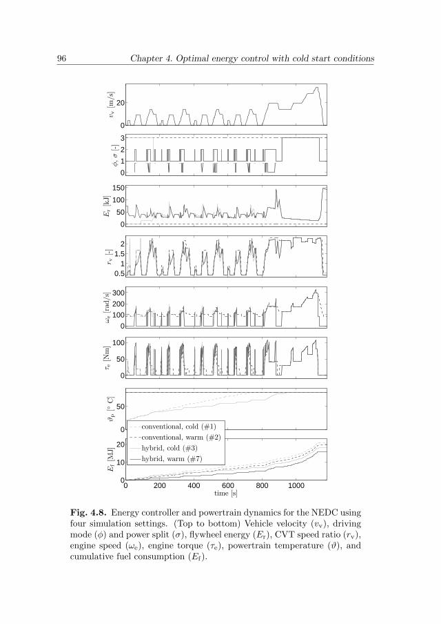
96 Chapter 4. Optimal energy control with cold start conditions
v v[m
/s]
0
20
φ,σ
[-]
0
1
2
3
Er
[kJ]
0
50
100
150
r v[-]
0.51
1.52
ωe
[rad
/s]
0
100
200
300
τ e[N
m]
0
50
100
ϑp
[C
]
0
50
Ef
[MJ]
time [s]
0 200 400 600 800 10000
10
20
conventional, cold (#1)
conventional, warm (#2)
hybrid, cold (#3)
hybrid, warm (#7)
Fig. 4.8. Energy controller and powertrain dynamics for the NEDC usingfour simulation settings. (Top to bottom) Vehicle velocity (vv), drivingmode (φ) and power split (σ), flywheel energy (Er), CVT speed ratio (rv),engine speed (ωe), engine torque (τe), powertrain temperature (ϑ), andcumulative fuel consumption (Ef).

4.7 Conclusions 97
v v[m
/s]
0
10
20
φ,σ
[-]
0
1
2
3
Er
[kJ]
0
50
100
150
r v[-]
0.51
1.52
ωe
[rad
/s]
0100200300
τ e[N
m]
0
50
100
ϑp
[C
]
0
50
Ef
[MJ]
time [s]
0 100 200 300 400 500 600 700 8000
10
20
conventional, cold (#1)
conventional, warm (#2)
hybrid, cold (#3)
hybrid, warm (#7)
Fig. 4.9. Energy controller and powertrain dynamics for the EHV usingfour simulation settings. (Top to bottom) Vehicle velocity (vv), drivingmode (φ) and power split (σ), flywheel energy (Er), CVT speed ratio (rv),engine speed (ωe), engine torque (τe), powertrain temperature (ϑ), andcumulative fuel consumption (Ef).
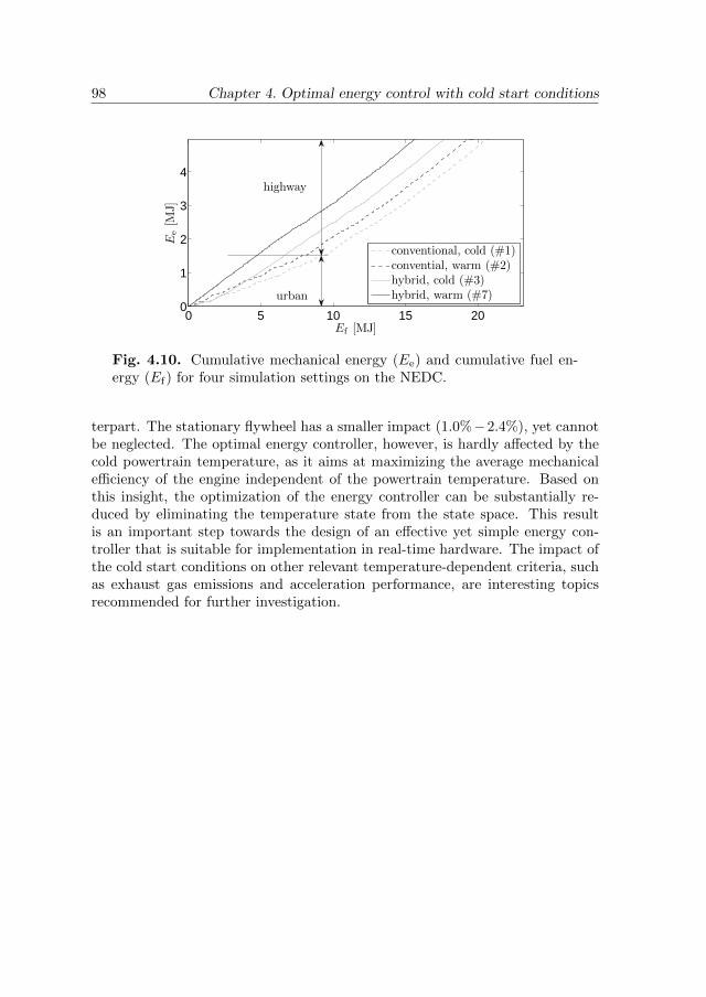
98 Chapter 4. Optimal energy control with cold start conditions
Ee
[MJ]
Ef [MJ]
0 5 10 15 200
1
2
3
4
conventional, cold (#1)convential, warm (#2)hybrid, cold (#3)hybrid, warm (#7)urban
highway
Fig. 4.10. Cumulative mechanical energy (Ee) and cumulative fuel en-ergy (Ef) for four simulation settings on the NEDC.
terpart. The stationary flywheel has a smaller impact (1.0%−2.4%), yet cannotbe neglected. The optimal energy controller, however, is hardly affected by thecold powertrain temperature, as it aims at maximizing the average mechanicalefficiency of the engine independent of the powertrain temperature. Based onthis insight, the optimization of the energy controller can be substantially re-duced by eliminating the temperature state from the state space. This resultis an important step towards the design of an effective yet simple energy con-troller that is suitable for implementation in real-time hardware. The impact ofthe cold start conditions on other relevant temperature-dependent criteria, suchas exhaust gas emissions and acceleration performance, are interesting topicsrecommended for further investigation.

Part II
Real-time control


Chapter 5
Real-time energy control withstatistical prediction
Abstract – This chapter presents the design of the energy controller for a mechanical hybrid
powertrain, that is suitable for implementation in real-time hardware. The design approach
follows a generic framework to i) solve the optimization problem using optimal control; ii)
make the optimal controller causal using a prediction of the future driving conditions; and iii)
make the causal controller robust by tuning of one key calibration parameter. The highly-
constrained optimization problem is solved with a numerical optimization algorithm known as
dynamic programming. The future driving conditions are modeled by a smooth approximation
of statistical data, and implemented in a receding horizon framework known as model predictive
control. The controller is made tunable by rule extraction based on physical understanding of
the system. The resulting rule-based controller is transparant, causal, and robust, as shown
by simulations for various driving cycles, start conditions, and calibration settings. The fuel
saving, however, is inherently sub-optimal, yet still very high for urban and mixed driving cycles
under warm start conditions (16.8% − 29.1%), and cold start conditions (12.6% − 22.8%).
5.1 Introduction
Hybrid powertrains have the potential to improve the fuel economy of passengervehicles significantly by adding a secondary power source to the internal combus-tion engine. A low-cost alternative to the state-of-the-art hybrid electric power-trains is a mechanical hybrid powertrain, which uses a compact flywheel systemfor kinetic energy storage and standard mechanical components such as a Con-tinuously Variable Transmission (CVT) and clutches for power transmission [8].The powertrain topology is schematically shown in Fig. 5.1. The flywheel sys-tem is mechanically connected by the CVT, which allows for smooth and efficient

102 Chapter 5. Real-time energy control with statistical prediction
Ce
Cf
Ct
vv
av τe
Pf
engine
CVT
rotor
flywheel system
wheels
gears
clutches
Fig. 5.1. Schematic representation of a mechanical hybrid powertrain.Different driving modes can be selected by using the engine clutch Ce
and the flywheel system clutch Cf . The transmission clutch Ct is used toaccelerate either the vehicle or the flywheel from standstill. The enginetorque (τe) determines the power split during hybrid driving, when boththe engine and flywheel system are engaged.
power transmission without energy conversion. The transmission clutch (Ct) hasthe conventional functionality to accelerate the vehicle from standstill while slip-ping, whereas the engine clutch (Ce) and flywheel system clutch (Cf) are usedto select a driving mode, by (dis-)engaging powertrain parts. The fuel savingbenefits can be attributed to three functionalities, which are i) recuperation ofbrake energy for later use, ii) elimination of inefficient part-load operation of theengine, and iii) engine shut-off during vehicle standstill.
5.1.1 Real-time energy control
To make full use of these functionalities, a controller is required, which controlson system level the power distribution between the engine, flywheel system, andvehicle. The main objective of this controller is to minimize the overall fuelconsumption for a given driving cycle, subject to the constraints imposed by thepowertrain dynamics, physical operating limits of the components, and drivingcomfort requirements. This energy controller may not rely on prediction systemsbased on inputs given by the driver (e.g., navigation), or sensors (e.g., global po-sitioning system, telemetry radar), in order to keep the cost of the hybrid systempotentially low. The controller may only use limited computation and memoryresources to be suitable for implementation in real-time hardware. Furthermore,the controller must be tunable to increase its robustness against measurementand prediction uncertainties. In order to enhance in-vehicle calibration, the con-troller design must be transparant to understand the impact of each calibrationparameter, whereas the number of calibration parameters needs to be as small

5.1 Introduction 103
as possible [22].
The design of such a real-time controller is widely studied in the literature, result-ing in several designs as described in [73]. Promising results are obtained usingsystematic design approaches that are based on optimal control. The generalapproach is to i) solve the optimal control problem offline using (semi-)analyticaloptimization methods; ii) make the controller causal using a prediction of thefuture driving conditions; and iii) make the controller robust, e.g., by calibrationof penalty functions or (feedback) control parameters. Often, a relatively simplehybrid electric powertrain is considered with a parallel topology, for which this(semi-)analytical approach is very suitable [37,104,105].
5.1.2 Main contributions and outline
The optimal control problem for a mechanical hybrid powertrain, however, istypically different due to i) switched dynamics (i.e., caused by the clutches) andii) active state constraints (i.e., caused by the small energy storage capacityand mechanical connections), and iii) non-convex control constraints to avoiduncomfortable driving mode switches. These characteristics make analytical op-timization unsuitable, yet numerical optimization can be used to follow the samedesign approach. Since numerical optimization methods generate a quantizedcontroller rather than an insightful analytical expression, rules need to be ex-tracted that approximate the generated control regions. When the extractedrules have a physically meaningful interpretation, insights can be gained in thedecision process, similar to the analytical expression. This numerical designapproach is also suitable for a more complex class of hybrid powertrains de-scribed by highly constrained, non-differentiable dynamics. It is expected thisclass of hybrid powertrains will increasingly emerge, using more driving modesto combine the benefits of several components in a complex topology (switcheddynamics), while downsizing the components to reduce cost (active state con-straints) without compromising comfort aspects (control constraints).
This chapter presents the design of a real-time controller for the consideredmechanical hybrid powertrain, following the optimal control-based design ap-proach. The optimal controller is computed with dynamic programming [18],whereas future driving conditions are considered in a model predictive controlframework [106], resulting in a time-invariant (causal) controller. The drivingconditions are predicted using a second order dynamic model based on proba-bility distributions from a set of representative driving cycles. Then, physicallyinterpretable rules are extracted to provide insights in the decision process andto enable calibration for robustness against uncertainty of predicted driving con-ditions, therewith following the philosophy of grounded theory [107]. Althoughthe controller is not yet implemented in real-time hardware, the two key chal-

104 Chapter 5. Real-time energy control with statistical prediction
lenges regarding causality and tunability will be addressed. In summary, themain contributions are
• classification of design methods based on optimal control in a genericframework;
• systematic design of a second order driving cycle model based on statistics;
• systematic design of a real-time controller for the highly-constrained me-chanical hybrid powertrain.
The outline of this chapter is as follows: Section 5.2 describes the classificationin a generic framework. Section 5.3 describes the design of the driving cyclemodel. Section 5.4 describes the modeling of the mechanical hybrid powertrain.Section 5.5 follows the design framework to design a real-time controller for themechanical hybrid powertrain. Section 5.6 discusses simulation results of thereal-time controller with respect to the optimal controller. Section 5.7 summa-rizes the results and conclusions.
5.2 Design framework for real-time energy con-troller
The design of a real-time energy controller based on optimal control is capturedin a generic design framework that consists of five steps:
1. define the optimal control problem;
2. classify the problem complexity;
3. solve the optimal control problem for prescribed driving cycles to optimizethe system design and its mathematical model;
4. solve the optimal control problem for a family of predicted driving cyclesto obtain a causal controller; and
5. tune the causal controller using calibration parameters for robustness againstmodeling and prediction uncertainty.
Below the five design steps will be discussed in more detail. Moreover, anoverview is given of possible solution methods found in literature for the differ-ent problem classes, as shown in Fig. 5.2. For each design step, it is importantto realize that approximations are (almost) unavoidable to make the problemsolvable, as indicated on the right hand side of this figure.

5.2 Design framework for real-time energy controller 105
real-time controller design
problem
problemcomplexity?
approximatedynamic
programming
stochasticdynamic
programming
ruleextraction
solution
minimumprinciple
equivalentconsumptionminimization
strategy
constraintrelaxation
deterministicdynamic
programming
modelpredictive
control
ruleextraction
design steps
1. formulationof cost function,dynamics, andconstraints
2. classificationof problemcomplexity
3. optimizationof designand model
4. predictionfor causality
5. calibrationfor robustnessagainstuncertainties
approximations
mathematicalmodeling
of physicalproblem
reductionof problem to
fit desired class
iteration orquantization
for feasibility
uncertaintyof future
conditions
abstractionof controller
for tunability
medium
low high
1
Fig. 5.2. Flowchart for the design of a real-time controller based onoptimal control. Problem complexity refers to the convexity of the optimalcontrol problem, the differentiability of the dynamics, and the activity ofthe constraints.
5.2.1 Problem formulation
The general optimal control problem is given by the minimization of a cost func-tion (e.g., fuel consumption, exhaust emission, acceleration performance), whichis described by a time-integral of the incremental cost g(x, u, w) as a function ofthe powertrain states x, control variables u, and external states w. The power-train dynamics are described by a differential equation using a dynamic functionf(x, u, w). The state space x ∈ X(w) is constrained to describe operating limitsof the powertrain, which may depend on the driving conditions w. The controlspace u ∈ U(x,w) is constrained to avoid undesired powertrain dynamics undercertain conditions (x,w), e.g., for comfort reasons. The external states describethe prescribed driving conditions (e.g., vehicle velocity and acceleration), andare limited to the external state space w ∈W . A discrete time format is assumedusing a fixed time step ∆ t, where k denotes the time index and kn denotes thefinal time index. The optimal sequence of control variables u∗(k) (or, optimalcontroller) is found by solving the optimal control problem:

106 Chapter 5. Real-time energy control with statistical prediction
u∗(k) = arg minu(k)
kn−1∑k=k0
g(x(k), u(k), w(k))∆t (5.1)
subject to
x(k0) = x0, (5.2)
x(k + 1) = x(k) + f(x(k), u(k), w(k))∆t, (5.3)
x ∈ X(w), (5.4)
u ∈ U(x,w), (5.5)
w ∈W, (5.6)
5.2.2 Classification of the optimal control problem
The problem complexity can be classified based on the characteristics of thedynamics, constraints, and cost function. The complexity of the dynamics isdetermined by its differentiability. Differentiable dynamics are suitable for ana-lytical optimization, whereas non-differentiable dynamics are more suitable fornumerical optimization. The linearity of the dynamics does not influence thecomplexity, but may improve the efficiency of the optimization solver. Thenumber of states does not influence the complexity, yet only determines thescale of the problem. The complexity of the constraints is determined by itsconvexity and activity, where the activity denotes to what extend the problem isdetermined by its constraints [108]. The convexity of the optimal control prob-lem is not only determined by the convexity of the constraints, but also by thatof the cost function and the concavity of the dynamics function [109]. Convexproblems with a low constraint activity are suitable for analytical optimization,whereas convex problems with a high constraint activity are suitable for dedi-cated (efficient) numerical optimization methods, whereas non-convex problemsare suitable for generic numerical optimization methods.
Based on these criteria, three problem classes are defined as schematically de-picted by the flowchart in Fig. 5.2: i) the problem class with a low complexity isdescribed by a convex problem with continuous dynamics subject to (relatively)inactive constraints (left), such as the power split problem for a hybrid electricpowertrain [37]; ii) the problem class with a medium complexity is described bya convex problem with switched dynamics subject to active constraints (mid-dle), such as the combined driving mode and power split problem for a hybridelectric powertrain [110]; and iii) the problem class with a high complexity isdescribed by a non-convex problem with switched dynamics subject to active

5.2 Design framework for real-time energy controller 107
constraints (right), such as the combined driving mode and power split problemfor a mechanical hybrid powertrain [66].
5.2.3 Optimization methods
The optimal control problem is deterministic when the complete driving cycleis exactly known beforehand, and can be solved using analytical methods basedon the Minimum Principle (MP) [15], or numerical methods based on DynamicProgramming (DP) [17]. The optimality of the controller does not considerapproximation errors introduced by mathematical modeling and iteration, orquantization errors introduced by the solvers. The optimal controller is suit-able i) for the optimization of the topology and component sizes of the hybridpowertrain [103], ii) for problem reduction by eliminating insignificant statesand control variables [111], and iii) as an optimization tool and performancebenchmark for a real-time controller.
5.2.3.1 Analytical optimization
Analytical optimization methods are based on Pontryagin’s MP to derive thenecessary conditions for optimality [16]. The methods adjoin the system dy-namics (5.3) with a multiplier function (or, adjoint state) to the incrementalcost function (5.1), leading to a function referred to as the Hamiltonian. Giventhe optimal multiplier function, the global optimal control problem can be re-duced to a local optimization of the Hamiltonian at each time instant. Theoptimal multiplier function is described by the Euler-Lagrange differential equa-tion, based on the Hamiltonian and state constraints [14]. Sequently, the opti-mal boundary values (initial and final) can be found for convex optimal controlproblems using iterative point-and-shoot methods [104, 112]. Given the opti-mal multiplier function, the analytical method gives a simple local optimizationproblem, which shows explicitly the decision between the actual cost and theequivalent cost of the system dynamics. Solving the Euler-Lagrange differentialequation, however, is not straightforward when dealing with active state con-straints [20] and non-differentiable (i.e., switched) dynamics [16], whereas theboundary value problem becomes complex when dealing with non-convex con-straints [109]. These problems can be avoided when approximating the problemby neglecting switched dynamics and state constraints except for the integralconstraint, as in [105].
5.2.3.2 Numerical optimization
Numerical optimization methods are based on Bellman’s DP, which uses theprinciple of optimality as a necessary condition for optimality [18]. The methodsexamine all the feasible state trajectory candidates, which satisfy the necessary

108 Chapter 5. Real-time energy control with statistical prediction
condition, by breaking down the global optimal control problem into local sub-problems for every (reachable) discrete state and time instant. This methodguarantees global optimality (with a quantization error) and produces a time-invariant control function for the given driving cycle [21]. The computationalcomplexity of the numerical method, in terms of computation time, is deter-mined by the number of feasible state trajectory candidates, which is hardlyinfluenced by the number and type of constraints (e.g, non-convex) or the typeof dynamics (e.g., switched, non-linear), but increases exponentially with thenumber of states and control variables. A course quantization would obviouslyreduce the computational time, but at the cost of sub-optimality, which can bepartly avoided by decomposing the problem [113], or by penalizing quantizationerrors in the local cost function [71]. Alternatively, the cost function and con-straints can be approximated to fit in a linear or quadratic programming frame-work [114], referred to as Approximate Dynamic Programming (ADP) [19,115],for which efficient solvers exist [116].
5.2.4 Causality by prediction
The optimal controller relies on the exact knowledge of the future driving con-ditions. This causality problem can be avoided by using a prediction of thefuture driving conditions based on current driving conditions w, instead of exactknowledge. Then, the analytical or numerical optimization methods can be usedto derive a causal controller as an explicit function of the powertrain and driv-ing cycle states (x,w). The prediction horizon kz can be selected as a trade-offbetween the prediction quality and the time scale of the powertrain dynamics,or stochastically by an absorbing state.
5.2.4.1 Equivalent consumption minimization strategy
The Equivalent Cost Minimization Strategy (ECMS) is derived from MP, whichgives a local optimization problem to minimize the momentary equivalent cost[117,118]. The multiplier function λ can be interpreted as an equivalence factorto express the state evolution as an equivalent cost, where predictions of fu-ture driving conditions w can be included in the multiplier function [119]. Thecontroller is found by solving
u∗(x,w) = arg minu∈U(x,w)
g(x, u, w) + λ(x, u, w)f(x, u, w), (5.7)
where the state constraints (5.4) are neglected here, but added in the sequel inthe form of soft constraints for the multiplier function.

5.2 Design framework for real-time energy controller 109
5.2.4.2 Stochastic dynamic programming
Stochastic Dynamic Programming (SDP) solves the optimal control problem fora family of stochastic driving cycles, which are described by statistical probabilitydistributions [110, 120, 121]. Since the method examines all possible stochasticdriving cycles, an efficient numerical solver is required, i.e., ADP. The controlleris found by solving
u∗(x,w) = arg minu∈U(x,w)
kz−1∑k=k0
E(εkg(x(k), u(k), w(k))), (5.8)
subject to the dynamics and constraints (5.3)-(5.5), where E denotes the expec-tation value and 0 < ε ≤ 1 denotes a discount factor that weights future costsexponentially less than current costs.
5.2.4.3 Model predictive control
The computational complexity of SDP can be substantially reduced by opti-mizing only the cost of an expected driving cycle, instead of optimizing theexpected cost for all possible stochastic driving cycles. Since the reduced opti-mization problem is a subset of the original optimization problem, a sub-optimalsolution is obtained. On the other hand, due to the reduced computational com-plexity, the more versatile DP can be used based on a more accurate model.The reduced optimization problem fits in the Model Predictive Control (MPC)framework [106,114,122,123], for which the explicit controller is found by solving
u∗(x,w) = arg minu∈U(x,w)
kz−1∑k=k0
g(x(k), u(k), E(w(k))) (5.9)
subject to the dynamics and constraints (5.3)-(5.5).
5.2.5 Robustness against uncertainties by calibration
The causal controller may be sensitive to uncertainties in the mathematicalmodeling of the original control problem and the prediction of the future driv-ing conditions. For robustness against these uncertainties, safety margins arerequired to avoid state constraint violation and to avoid unnecessary controldecisions. These safety margins needs to be tunable with only a few calibrationparameters, of which the impact is understandable and effective, in order toreduce the (in-vehicle) calibration effort.

110 Chapter 5. Real-time energy control with statistical prediction
5.2.5.1 Constraint relaxation
The causal controller obtained with ECMS approximates the original controlproblem by neglecting state constraints and by the (incorrect) prediction offuture driving conditions. These uncertainties are transferred to an uncertaintyin the optimal multiplier value λ(k). From (5.7) it follows that an error in themultiplier function has an integrating effect on the state evolution f(x, u, w)such that state constraint violation is unavoidable at some time instant. Thisproblem can be avoided by introducing soft constraints on the multiplier function[73], e.g., in the form of a penalty function [124], or a state-feedback controller[37]. This constraint relaxation of the original hard constraints given by (5.4)is obviously sub-optimal, yet acceptable when the constraint activity is low.Moreover, the relaxation of the integral constraint for energy sustenance (i.e.,x(kn) ≈ x(k0)) can be considered even more “natural”, than a hard constraintat the final time instant (i.e., x(kn) = x(k0)).
5.2.5.2 Rule extraction
The causal controller obtained with MPC or SDP is described by a (multi-dimensional) matrix, of which each element describes the control variable as afunction of the quantized powertrain and driving conditions (x,w). The controlmatrix is typically characterized by control regions, where neighboring elementshave the same control variable. Uncertainty about future driving conditionsis transferred to uncertainty in the shape of these regions. In addition, non-smooth irregularities may occur due to the quantization and the use of a finiteprediction horizon, such that instantaneous costs (e.g., engine cranking) can bejust postponed beyond the horizon under certain conditions. Such irregulari-ties are obviously not desired for a smooth and consistent powertrain response.These problems can be avoided by extracting rule functions that approximatethe boundaries of the control regions [124–126]. Sequently, the control regionscan be tuned without computing the control matrices again. When the rule ex-traction is based on physical understandings of the system, insights are gained inthe implicit decision process of the numerical controller, which is very useful toidentify the key calibration parameters to increase the robustness against model-ing and prediction uncertainties. The abstraction process of this rule extractionfollows both inductive and deductive reasoning, as in-depth understanding ofthe system is exploited to explain the causal controller data, whereas system un-derstanding is also generated from the analysis of this data, therewith followingthe philosophy of grounded theory [107].

5.3 Driving cycle modeling 111
5.3 Driving cycle modeling
The future driving conditions are modeled by a second order dynamic model,using only statistical information from a set of representative driving cycles toavoid (relatively costly) integration of prediction systems such as navigation andcruise control.
5.3.1 Driving cycles
A set of six representative driving cycles is selected: the New European Driv-ing Cycle (NEDC), the Japan Cycle 08 (JC08), the Federal Test Procedure’75 (FTP75), the “low”, “medium”, and “high” parts of the Worldwide har-monized Light vehicles Test Procedure (WLTP), the “urban” part of the Com-mon Artemis Driving Cycle (CADC), and the sportive Eindhoven driving cycle(EHV). The JC08, NEDC, and FTP75 are selected to represent certified driv-ing cycles for certified fuel consumption measurements in the most importantcontinents of the automotive industry, i.e., Asia, Europe, and North-America,whereas the WLTP, CADC, and EHV represent real-world driving behaviormeasured in, respectively, worldwide industrialized countries [79], Europe [80],and Eindhoven (The Netherlands) as shown in Chapter 3. Since the flywheelsystem is aimed for urban use, highway cycles such as the “extra high” part ofthe WLTP and the “‘extra urban” and “highway” parts of the CADC are notconsidered. The driving cycles describe, as the majority of the driving cyclesfound in the literature, only variations in velocity. Nevertheless, the presentedmodeling method can be extended by considering other variations such as inaltitude, wind, and road surface quality.
5.3.2 Dynamics and constraints
The driving conditions determine through an inverse dynamics model the re-quired rotational speed and torque at the drive shaft of the hybrid powertrain,which are described by two states, i.e., the vehicle velocity vv and vehicle ac-celeration av. The dynamics of these states can be described by two first-orderdifference equations, using a time step of ∆t = 1 s, as a function of an externalstate that describes the change in acceleration (or, jerk) jv, by
vv(k + 1) = vv(k) + av(k)∆t, (5.10)
av(k + 1) = av(k) + jv(k)∆t, (5.11)
where k ∈ [k0, kn − 1] denotes the time index. The dynamics is constrainedby the physical limitations of the vehicle, which restricts the velocity rangevv ∈ [vv, vv] and the velocity-dependent acceleration range av ∈ [av(vv), av(vv)]

112 Chapter 5. Real-time energy control with statistical prediction
(see, Fig. 5.3). The velocity-dependent acceleration range can be approximatedby a fourth-order polynomial function of the velocity:
av(vv) = ccs,1 + ccs,2vv + ccs,3v2v + ccs,4v
3v + ccs,5v
4v,
av(vv) = −av(vv), (5.12)
where the coefficients ccs are identified using a standard least-square fittingmethod and listed in Table 5.1. The state constraints can be expressed as explicitconstraints on the jerk prediction jv ∈ [j
v(av, vv), jv(av, vv)], by
jv(vv, av) = max
vv − vv − 2av∆t
∆t2,av − av
∆t
,
jv(vv, av) = min
vv − vv − 2av∆t
∆t2,av − av
∆t
. (5.13)
5.3.3 Prediction
The jerk jv can be predicted based on present information (vv, av), where arelatively short prediction horizon of 10−20 s is sufficient to predict the relevantdynamics of the energy buffer, due to the relatively small energy storage capacityof the flywheel system. Below, three methods are evaluated to derive a predictionfor the jerk jv.
5.3.3.1 Constant acceleration
Under normal driving conditions, the driver is quite capable to anticipate thedriving conditions in the near future, which enables the driver to regulate thevehicle acceleration with only limited variations in acceleration (or, jerk) toobtain a high comfort level. Assuming that the driver succeeds in such drivingbehavior, by keeping the accelerator (or, brake) pedal approximately constant,the jerk is predicted by a straightforward model
jv(vv, av) = 0. (5.14)
5.3.3.2 Statistical expectation
Instead of assuming a certain driving behavior, it can also be extracted from aset of representative driving cycles. The probability distributions of the jerk canbe obtained for a quantized velocity, acceleration, and time. Using the indices i1and i2 for, respectively, the quantized velocity and acceleration, the expectationvalue of the jerk can be computed as a function of the quantized velocity andacceleration by

5.3 Driving cycle modeling 113
jv(vv(i1), av(i2)) =
∑knk=k0
n1(i1, i2, k)jv(k)∑knk=k0
n1(i1, i2, k),
n1(i1, i2, k) :=
1 if bvv(k)e = vv(i1) ∧ bav(k)e = av(i2),
0 else,(5.15)
where b·e denotes rounding towards the nearest discrete state and n1(i1, i2, k) canbe considered as a conditional sampler. The resulting phase portrait is depictedin the middle graph of Fig. 5.3, where the lines denote, in clockwise direction,the change in phase and magnitude during one time step (1 s). The circlesdenote local equilibria, for which av ≈ 0 m/s2 and jv ≈ 0 m/s3 holds, which canbe interpreted as (approximately) constant velocities. The phase portrait showsin general smooth dynamics, except for local discontinuities (i.e., crossing lines)
due to the limited number of samples, i.e., when∑knk=k0
n1(i1, i2, k) << 50. Forits purpose in the design of a real-time controller, however, a smooth predictionis required for a consistent powertrain response.
5.3.3.3 Approximated expectation
The discontinuities of the statistical probability method can be “smoothed” byapproximating the expected jerk by a semi-empirical model function. The modelfunction describes the main dynamical characteristics, such as the symmetryaround the zero acceleration axis, a high positive jerk at low velocities, no jerkaround vv ≈ 6 m/s, and a negative jerk that slowly attenuates at higher veloci-ties. These dynamics are approximated by the function:
jv(vv, av) =(cdc,1 + cdc,2vv + cdc,3v
2v + cdc,4v
3v
)(cdc,5 + cdc,6av + cdc,7a
2v
)ecdc,8vv , (5.16)
where the coefficients cdc are identified using a standard least-square fittingmethod, and listed in Table 5.1. The resulting phase portrait is depicted inthe bottom graph of Fig. 5.3. As can be seen, the empirical model functionapproximates the expected dynamics quite well.
5.3.4 Results
Examples of the predictions are shown in Fig. 5.4, for the constant accelerationmodel (5.14) and the approximated expectation model (5.16). The top left andthe middle left graphs show constant driving conditions for both models, whichcorrespond to the local equilibria in the phase portrait in Fig. 5.3, whereas the

114 Chapter 5. Real-time energy control with statistical prediction
av
[m/s
2]
−2
−1
0
1
2
vv [m/s]
av
[m/s
2]
0 5 10 15 20 25 30−2
−1
0
1
2
av
[m/s
2]
−2
−1
0
1
2
constant acceleration
statistical expectation
approximated expectation
Fig. 5.3. Phase portraits of the driving cycle dynamics based on a con-stant accelerator pedal (top graph), statistical probability (middle graph)and an empirical model function (bottom graph). The lines denote, inclockwise direction, the phase and magnitude change of the states (i.e.,dynamics) for one time step (1 s). The circles denote local equilibria, forwhich av ≈ 0 m/s2 and jv ≈ 0 m/s3 holds.
top right and the bottom right graphs show (almost) fully constrained predic-tions due to (5.12), where av ≈ av. For the remainder of the situations, themodels give rather different predictions.
The prediction quality of the two models is evaluated for several predictionhorizons kz. The prediction error is expressed by the difference between theactual and predicted propulsion energy, which should be small compared tothe storage capacity of the flywheel system to foresee possible state constraintviolations. The propulsion energy can be computed using a model that describesthe required wheel power Pw(vv, av) to track the velocity profile of the drivingcycle. From a given time instant k0 of a known driving cycle, the predictionerror starts with Ew(k0) = 0 and proceeds with
Ew(k + 1) = Ew(k) + (Pw(vv(k), av(k))− Pw(vv(k), av(k))) ∆t, (5.17)

5.3 Driving cycle modeling 115
time [s]0 20 40
time [s]0 20 40
time [s]
v v[m
/s]
0 20 400
10
20
30
v v[m
/s]
0
10
20
30
av(k0)=1.5m/s2av(k0)=0.5m/s2av(k0)=0m/s2
v v[m
/s]
0
10
20
30 constant accelerationapproximated expectation
Fig. 5.4. Examples of predictions based on a constant pedal assumptionand based on a functional approximation of the statistical expectation.The graphs show, from top to bottom respectively, different initial veloc-ities vv(k0) ∈ 0, 5, 15 m/s, and from left to right respectively, differentinitial accelerations av(k0) ∈ 0, 0.5, 1.5 m/s2.
for k = k0, k + 1, . . . , k + kz − 1. The maximum prediction error within thehorizon follows as
Ew(k0, kz) := maxk∈[k0,mink0+kz,kn]
|Ew(k)|. (5.18)
The average maximum prediction error Ew(kz) is given for the relevant urban,non-standstill and non-braking parts of the entire driving cycle, by
Ew(kz) :=
∑knk=k0
n2(k)Ew(k, kz)∑knk=k0
n2(k),
n2(k) :=
1 if 0 < vv(k) < vu ∧ av(k) ≥ 0,
0 else,(5.19)
where n2(k) can be considered as a conditional sampler and vu = 13.89 m/s(50 km/h) denotes the maximum urban velocity. Fig. 5.5 shows some results

116 Chapter 5. Real-time energy control with statistical prediction
Ew(k
z)/
Er
[%]
0
20
40
60 constant acceleration (kz=10)approximated expectation (kz=10)
Ew(k
z)/
Er
[%]
0
50
100
150 constant acceleration (kz=20)approximated expectation (kz=20)
Ew(k
z)/
Er
[%]
NEDC JC08 WLTP FTP75 CADC EHV0
100
200
300constant acceleration (kz=40)approximated expectation (kz=40)
Fig. 5.5. Average maximum prediction error in terms of propulsionenergy (Ew(kz)) with respect to the energy storage capacity of the flywheelsystem (Er), for the relevant non-standstill and non-braking, urban partsof the driving cycles.
of the average maximum prediction error for a compact vehicle (1120 kg) withrespect to the energy storage capacity of the flywheel system Er (150 kJ), forthe two prediction models using three horizons, i.e., kz ∈ 10, 20, 40. As ex-pected, the prediction error increases with the prediction horizon and with the“sportiveness” of the driving cycle (i.e., velocity variations). For a relativelyshort prediction horizon (i.e., kz=10), both prediction models give similar re-sults, where the constant acceleration model even outperforms the approximatedexpectation model for the stylistic NEDC. For other driving cycles or longer pre-diction horizons, the approximated expectation model outperforms the constantacceleration model up to a factor of 3. The average maximum prediction errorexceeds 50% of the energy storage capacity of the flywheel system for predictionhorizons higher than 20 s for all driving cycles, which can therefore be consideredas an upper bound for a the controller design.
The presented prediction methods rely on an inverse dynamics model to computethe wheel power (Pw), while in practice, the vehicle velocity is controlled by thedriver through the accelerator pedal. Hence, for in-vehicle implementation ofthis prediction model, a low-pass filter may be required to reduce the impact

5.4 Mechanical hybrid powertrain modeling 117
Table 5.1. Driving cycle model coefficients.
jerk model acceleration constraints
coefficient value coefficient value
cdc,1 1.20 ccs,1 −8.77 · 10−6
cdc,2 −3.75 · 10−1 ccs,2 9.01 · 10−4
cdc,3 6.23 · 10−2 ccs,3 −2.97 · 10−2
cdc,4 −6.28 · 10−3 ccs,4 2.78 · 10−1
cdc,5 2.22 · 10−1 ccs,5 1.58cdc,6 −2.33 · 10−2
cdc,7 1.93 · 10−1
cdc,8 −2.44 · 10−1
of high-frequent variations such as pedal jogging (and noise) in the measuredacceleration signal (av) on the predicted driving conditions.
5.4 Mechanical hybrid powertrain modeling
The mechanical hybrid powertrain consists of a 4-cylinder 1.5-l gasoline internalcombustion engine, a vacuum-placed 150-kJ flywheel system, three clutches, amass-produced pushbelt CVT, and a compact vehicle including 2 passengerswith a total mass of 1120 kg, as schematically depicted in Fig. 5.1.
5.4.1 Dynamics
The modeling of the constrained dynamics is extensively described in Chapter 3and shortly summarized in the sequel. The motion dynamics is extended withthe powertrain thermodynamics using the model described in Chapter 4, to showthe impact of cold start conditions on the fuel consumption. The longitudinaldynamics are described for the most relevant (largest) inertias, i.e., that of theflywheel and the vehicle. The transmission clutch (Ct) is used to transmit hightorques while slipping, e.g., to accelerate the vehicle from standstill. The engineclutch (Ce) and the flywheel system clutch (Cf) are not designed to transmithigh torques whiles slipping, yet to select driving modes by mechanical (dis-)engagement of powertrain parts. The powertrain can be operated in threerelevant driving modes:
• Flywheel driving : the flywheel propels or brakes the vehicle while the en-gine is shut-off (φ = 1).
• Hybrid driving : the engine and flywheel propel the vehicle, where thecontribution of each power source is determined by the relative power split

118 Chapter 5. Real-time energy control with statistical prediction
(φ = 2).
• Engine driving : the engine propels the vehicle while the flywheel is coast-ing, whereas the flywheel brakes the vehicle while the engine is idling(φ = 3).
The combined motion dynamics and thermodynamics can be described with onedynamic function cf. 5.3, where the state vector x(k) contains the kinetic energyin the rotor of the flywheel system (or, flywheel energy) Er(k), the previousdriving mode φpre(k) = φ(k − 1), and the powertrain temperature ϑp(k). Thecontrol variables u(k) are the current driving mode φ(k) and the relative powersplit σ(k) in the hybrid driving mode, which is defined as the torque reservefraction of the engine used to energize the flywheel system:
σ :=τe − τp
τ e(ωe)− τp. (5.20)
Here, τe denotes the generated engine torque, τ e(ωe) denotes the maximumengine torque as a function of the rotational speed ωe, and τp denotes the torqueat the primary side of the CVT. So, σ < 0 implies boosting of the engineusing the flywheel, σ = 0 implies coasting of the flywheel, and σ = 1 impliesmaximal energizing of the flywheel. The external state vector w(k) contains thevehicle speed vv(k) and the acceleration av(k), prescribed by the driving cycleor predicted by a driving cycle model.
5.4.2 Constraints
The dynamics are constrained by state constraints based on physical operationlimits of the components, and control constraints to guarantee a high comfortlevel.
5.4.2.1 State constraints
The engine speed ωe and engine torque τe are constrained by
ωe ∈ 0, ωidle, [ωe, ωe], (5.21)
τe ∈ [0, τ e(ωe)]. (5.22)
The engine is either shut-off (ωe = 0), or idling without generating power atvehicle standstill (i.e., ωe = ωidle), or generating power (i.e., ωe ∈ [ωe, ωe]).Physically, the engine can generate a negative torque by its friction, but that isnot relevant for the controller design. The transmission operation is describedby the rotational speeds ω and torques τ on both side of the transmission, i.e.,

5.4 Mechanical hybrid powertrain modeling 119
the primary (or, engine) side indicated by subscript “p” and the secondary (or,drive shaft) side indicated by the subscript “s”. The speeds and torques havephysical limitations, which are not critical for the controller design, except forthe speed ratio rv = ωs/ωp:
rv ∈ [rv, rv]. (5.23)
The flywheel system operation is described by the flywheel energy, which isconstrained by
Er ∈ [0, Er]. (5.24)
After the initialization of the flywheel system, the flywheel energy should exceeda lower bound Er > Er > 0, as will be described in the sequel.
5.4.2.2 Control constraints
The powertrain response must be fast and smooth, with an acceptable consis-tency of the engine noise. In order to guarantee this level of driving comfort,some dynamics must be avoided under certain conditions (x,w), by constrainingthe control space U . A state-dependent control space U(x,w) generally limitsthe feasible state space X(w) to a non-convex subset of the unconstrained statespace. An example of such a non-convex control constraint is the irreversibledriving mode switch from hybrid driving φ = 2 (or, flywheel driving φ = 1) toengine driving φ = 3. Fast and smooth disengagement of the flywheel systemclutch (Cf) is always possible (i.e., φpre = 2 ∧ φ = 3), but fast and smoothengagement (i.e., φpre = 3∧ φ = 2) is only possible when no torque is transmit-ted, i.e., when braking with the disc brakes, since the clutch is not designed todissipate high powers. The second control constraint guarantees a fast torquegeneration of the engine after flywheel driving, e.g., to handle change-of-mindactions of the driver. This requires a minimum effective flywheel speed, or im-plicitly a minimum effective flywheel energy Er, in order to crank the engine tothe minimum engine speed ωe cf. (5.21), so Er ≥ Er must hold in the flywheeldriving mode (φ = 1). The same constraint holds for the hybrid driving mode(φ = 2), in order to generate sufficient torque for vehicle propulsion. The thirdcontrol constraint is related to the engine noise, which may be counterintuitiveto the driver as its frequency rises when energizing the flywheel during hybriddriving (φ = 2). For an acceptable consistency of the engine noise, hybrid driv-ing is avoided when no propulsion torque is required τp ≤ τ0 to keep the noiselevel low, where τ0 denotes a threshold close to zero, and outside urban areasvv > vu to limit engine noise variations that result from duty-cycle switchingbetween hybrid and flywheel driving. These constraints are summarized in thedriving mode control space, given by

120 Chapter 5. Real-time energy control with statistical prediction
φ ∈
3 if Er < Er ∨ (φpre 6= 3 ∧ τp > τ0),
1, 3 else if τp ≤ τ0 ∨ (φpre 6= 2 ∧ vv > vu),
1, 2, 3 else.
(5.25)
Since boosting of the engine (σ < 0) does in general not contribute to a lowerfuel consumption, as the engine is usually more efficient at high torques, therelative power split control space can be reduced to
σ ∈ [0, 1]. (5.26)
5.5 Controller design
The generic design framework as described in Section 5.2 is used to design areal-time controller for this mechanical hybrid powertrain.
5.5.1 Problem formulation
The optimal control problem is to minimize the overall fuel energy consumption(Ef) for a given driving cycle, where Pf denotes the fuel power (chemical energyflux), given by
u∗(k) = arg minu(k)
kn−1∑k=k0
Pf(x(k), u(k), w(k))∆t, (5.27)
subject to the system’s dynamics (5.3), (5.20), and (comfort-related) constraints(5.21)-(5.26). There is no final state constraint for energy sustenance, as theflywheel system can only store energy for a relatively short term (< 30 min.).Nevertheless, even without the final state constraint, the final energy level isusually non-zero, due to brake energy recuperation at the end of the drivingcycle, and due to energy constraints for driving modes other than engine driving(see, (5.25)).
5.5.2 Classification
The mechanical hybrid powertrain is characterized by switched dynamics, non-convex control constraints (5.25), and active state constraints (5.24) due to thesmall energy storage capacity of the flywheel system, and due to its fixed connec-tion with the transmission (5.23) and engine (5.21), (5.22). This optimal controlproblem is classified as complex, so DP is selected for the optimization, MPC is

5.5 Controller design 121
selected for the causal controller design, and rule extraction is selected to obtaina rule-based (RB) controller, which is suitable for real-time implementation andcalibration, cf. the flow chart in Fig. 5.2.
5.5.3 Optimal controller
From previous research, it follows that the optimal control problem can be sub-stantially reduced with only a minor impact on the solution, by reducing thestate space X and the control space U . The state space can be reduced byneglecting the powertrain temperature ϑp [111], whereas the control space canbe reduced by selecting only power splits that are essential for the functionalityof hybrid driving, which are i) efficient energizing of the flywheel system andii) maintaining control flexibility, e.g., to avoid the irreversible switch to enginedriving [66]. These two functionalities can be captured by only two power splitvalues, given by
σ ∈ 0, σ∗, (5.28)
where σ = 0 can be interpreted as the hybrid variant of engine driving, whilemaintaining the control flexibility to switch to other driving modes. The en-ergizing power split σ∗ := σ(τe = τ∗e ) corresponds to the statically optimizedengine torque
τ∗e := arg minτe
(Pf(ωe, τe)
τeωe
), (5.29)
where the engine speed ωe is kinematically determined by the flywheel energy.
5.5.4 Causal controller
The controller is made causal by using the MPC framework given by (5.9) andthe prediction model given by (5.10)-(5.13) and (5.16). The prediction horizon kz
must be short to keep the prediction error small, yet sufficiently long to includethe relevant powertrain dynamics, so that momentary switching costs are spreadover the driving mode duration, and forced mode switches in the near future(due to constraints) are considered. The upper bound of the prediction horizonfollows from the prediction error of the driving cycles as shown in Fig. 5.5, andis determined at 20 time instants. The lower bound is determined by the timeconstant of the powertrain dynamics, which is quantified as the average timespent in a driving mode using the optimal controller obtained with DP. For therelevant urban, non-standstill and non-braking parts of a given driving cycle,the time constant kp is given by

122 Chapter 5. Real-time energy control with statistical prediction
Table 5.2. Average time spent in driving mode1.
Driving cycle: NEDC WLTP JC08 FTP75 CADC EHV
kp∆t [s] 11.2 10.2 9.2 9.1 8.4 7.5
1obtained with the optimal controller (DP) for the urban, non-standstill, andnon-braking parts of the driving cycles.
kp :=
∑knk=k0
n2(k)∑knk=k0
n2(k)n3(k), n3(k) :=
1 if φ(k) 6= φpre(k)
0 else, (5.30)
using the conditional sampler n2(k) given by (5.19), and is listed for variousdriving cycles in Table 5.2. As expected, the time constant is relatively short(on average, 9 time instants), due to the small energy storage capacity and thehigh constraint activity, and decreases with the sportiveness of the driving cycle(i.e., velocity variations). The prediction horizon is selected between the upperand lower bound, as kz = 15.
A part of the resulting controller u∗(x,w) is shown in Fig. 5.6 as a functionof the driving cycle states (vv, av), for given powertrain states (Er = 25 kJ,φpre = 1). To give a clear overview, only “steady” control variables are shownthat remain unchanged for at least 3 time instants for the predicted drivingcycle. As expected, several control regions can be distinguished, where somenon-smooth irregularities can be observed due to momentary costs caused bythe switched dynamics and a finite prediction horizon. In general, the followingcontrol decisions can be observed: for high power demands (vv >> 0, av >> 0),the engine is efficiently operated in the engine mode. For low and negative powerdemands, the flywheel is used for propulsion and braking. For intermediatepower demands, both the flywheel and engine are engaged in the hybrid mode.A general behavior of the power split, however, is not clear from this perspective.
5.5.5 Rule-based controller
Rules are extracted from the causal (MPC) controller based on physical under-standing of the hybrid powertrain, and calibrated for robustness against the pre-diction error. Two types of rules can be distinguished, i.e., feasibility rules andoptimality rules, as will be explained in the sequel. Subsequently, the rule-based(RB) controller design is described for which one suitable calibration parameteris assigned to increase its robustness against the prediction uncertainty.

5.5 Controller design 123
vv [m/s]
av
[m/s
2]
0 5 10 15 20 25 30−1
−0.5
0
0.5
1
1.5
2
2.5φ = 1φ = 2φ = 2φ = 3
rv vu rv
τ0
τ e
Fig. 5.6. MPC result as a function of the vehicle velocity vv and acceler-ation av, for a given relative flywheel energy of Er/Er = 17% and drivingmode state φpre = 1. Uncertain control variables that change within 3time instants are not shown. The lines denote active constraints, givenby the speed ratio limits rv and rv, the urban velocity limit vu, the min-imum propulsion torque τ0, and the engine torque limit τ e. The controlvariables in the grey areas are purely determined by the constraints.
5.5.5.1 Feasibility rules
The feasibility rules restrict the control space by the operating limits of thehybrid powertrain. The rules are given by the constraints (5.21)-(5.25) and(5.28), and illustrated by lines in Fig. 5.6. Some of the rules restrict the controlspace to only one possible control decision for a part of the state space, whichis indicated by the grey areas. The relatively large grey areas reflect the highconstraint activity of this powertrain. The remainder of the state space (whitearea) requires additional rules to make a distinct control decision. Althoughthe feasibility rules are fixed by the physical powertrain characteristics, a smallsafety margin may be required for robustness against sensor and estimationuncertainty.
5.5.5.2 Optimality rules
The optimality rules control the energy dynamics in order to optimize the costfunction for the predicted driving conditions. These rules are related to the fly-wheel energy range given by (5.24) and the predicted driving conditions. Twosets of rules are distinguished: one set to choose the driving mode φ, and oneset to choose the power split σ. The power split rules make the decision betweenflywheel coasting (σ = 0) and flywheel energizing (σ = σ∗), and is based on theobservation that energizing is only effective when i) the engine is operated atan inefficient low torque otherwise, ii) the flywheel energy level is low, and iii)

124 Chapter 5. Real-time energy control with statistical prediction
the transmission clutch (Ct) is engaged, to limit the power dissipation of theslipping clutch. These rules are described by (5.33) next.
The driving mode rules make the decision between flywheel driving (φ = 1)and hybrid driving (φ = 2), therewith avoiding the irreversible switch to enginedriving, if feasible. Engine driving (φ = 3) is therefore only used for feasibility.The rules are based on the predicted propulsion energy for a given predictionhorizon kz, which is given by
Er(kz) =
kz−1∑k=k0
f1(x(k), u(k), w(k))∆t |φ=1, (5.31)
where f1 denotes the part of function f in (5.3) that describes the dynamicsof the flywheel energy state. The available flywheel energy is given by Er, forwhich an additional offset Eo and hysteresis band Ehyst are introduced for fitting
purposes. The resulting energy balance Er = Er+Eo+Ehyst can be used as a ruleto decide whether sufficient energy is available for flywheel driving (φ = 1), anddecides hybrid driving (φ = 2) otherwise. The prediction horizon kz (differentfrom the one used with MPC), the offset Eo and the hysteresis band Ehyst, areobtained by fitting the energy balance with the MPC result. Fig. 5.7 shows theMPC result as a function of the flywheel energy (Er) and the predicted energyconsumption (Er). Each of the four graphs depicts one control decision (eitherφ = 1 or φ = 2) for one driving mode state (either φpre = 1 or φpre = 2), whereasthe energy balance is depicted by the diagonal lines. The vertical offset of theselines is determined by either Eo or Eo + Ehyst, whereas the slope is related tothe prediction horizon kz. It can be seen that the energy balance separates thecontrol decisions quite well, using the fitted parameters as listed in Table 5.3.The hysteresis band Ehyst gives a different energy balance for the hybrid drivingmode (φ = 2) than for the flywheel driving mode (φ = 1), thereby dampingagainst switching between the driving modes. As an additional rule, when thepredicted propulsion energy using a prediction horizon off only one time step(i.e., Er(1)) exceeds the effective energy left in the flywheel (i.e., Er − Er), thecontroller must switch to hybrid driving (φ = 2). This situation covers themismatch indicated by the ellipse on the left bottom of Fig. 5.7.
5.5.5.3 Controller design
Combining the feasibility and optimality rules, where the priority of each rule ismainly determined by the feasibility, the following RB controller is obtained:

5.5 Controller design 125
Er/E
r[%
]φpre=1
0
50
100E
r/E
r[%
]
Er(kz)/Er [%]0 50 100
0
50
100
φ = 1φ = 2φ = 2
φpre=2
φ = 1φ = 2
Er(kz)/Er [%]0 50 100
Er
Er
Eo
Eo
Eo + Ehyst
Eo + Ehyst
Fig. 5.7. Causal controller obtained with MPC as a function of the pre-dicted flywheel energy consumption Er and the available flywheel energyEr. The energy balance of the RB controller is shown by the diagonallines.
φ =
3 if Er ≤ Er
1 else if τ ′p ≤ τ03 else if φpre = 3 ∨ r′v ≥ rv ∨ τ ′p > τ e
1 else if Er > Er(1) + Er, ∧(
(φpre = 1 ∧ Er > Er(kz) + Eo) ,
∨ (φpre = 2 ∧ Er > Er(kz) + Eo + Ehyst))
3 else if φpre = 1 ∧ vv > vu
2 else
,
(5.32)
σ =
σ∗ if r′v ≥ rv ∧ τp ≤ Er−Er
Er−Er
τ∗e
0 else, (5.33)
where r′v = rv | φ = 1 and τ ′p = τp | φ = 1 denote, respectively, thespeed ratio and the primary torque for a (virtually) engaged flywheel clutch.The associated control regions are shown in Figs. 5.8 and 5.9 by the grey areas,together with the control regions obtained with MPC (symbols). From the

126 Chapter 5. Real-time energy control with statistical prediction
av
[m/s
2]
Er/Er=17%
−1
0
1
2
Er/Er=29% Er/Er=40%
av
[m/s
2]
Er/Er=52%
−1
0
1
2
Er/Er=64%
vv [m/s]
Er/Er=76%
0 20
vv [m/s]
av
[m/s
2]
Er/Er=88%
0 20−1
0
1
2
vv [m/s]
Er/Er=100%
0 20
φ = 1φ = 2, σ = 0φ = 2, σ = σ∗
φ = 3
Fig. 5.8. Explicit RB and MPC controllers for φpre = 1 as a functionof the vehicle velocity vv, acceleration av, flywheel energy Er, and thedriving mode state φpre. The RB control regions are indicated by thegrey areas (see, legend Fig. 5.9), whereas the MPC control regions areindicated by the symbols.
graphs, it can be seen that the RB controller gives a smooth approximation ofthe control regions obtained with MPC. Besides the substantial simplification,the RB controller can be calibrated relatively easily, by using only one calibrationparameter, i.e., the hysteresis band Ehyst, as will be described below.
5.5.5.4 Calibration parameter
The damping of the hysteresis band Ehyst is required to limit the energy costto crank the engine, when switching from flywheel driving to hybrid driving.Besides the fuel benefit, the hysteresis also contributes to a more consistentpowertrain response. However, a large hysteresis band increases the averageflywheel energy, thereby increasing the operating speeds of the powertrain com-ponents and the associated frictional energy dissipation, so there is a trade-off.Using MPC, this trade-off is found by operating the flywheel energy close to itsminimum (Er), while unnecessary driving mode switches are precisely avoided

5.6 Results and discussion 127
av
[m/s
2]
Er/Er=17%
−1
0
1
2
Er/Er=29% Er/Er=40%av
[m/s
2]
Er/Er=52%
−1
0
1
2
Er/Er=64%
vv [m/s]
Er/Er=76%
0 20
vv [m/s]
av
[m/s
2]
Er/Er=88%
0 20−1
0
1
2
vv [m/s]
Er/Er=100%
0 20
φ = 1φ = 2, σ = 0φ = 2, σ = σ∗
φ = 3
Fig. 5.9. Explicit RB and MPC controllers for φpre = 2 as a function ofthe vehicle velocity vv, acceleration av, flywheel energy Er, and the drivingmode state φpre. The RB control regions are indicated by the grey areas,whereas the MPC control regions are indicated by the symbols (see, legendFig. 5.8).
for the predicted driving cycle. This strategy works well if the actual drivingconditions precisely match with the prediction. However, when this is not thecase, each time when the flywheel energy reaches its minimum, “unnecessary”driving mode switches are unavoidable. This sensitivity against prediction un-certainties can be reduced by selecting a higher hysteresis band such that theflywheel energy is operated further from its minimum. As a result, the hysteresisband Ehyst serves as useful calibration parameter to add robustness, but at thecost of a higher fuel consumption. This calibration parameter is easily adaptedin the RB controller and allows for in-vehicle calibration.
5.6 Results and discussion
Simulations are performed to evaluate the performance of the RB real-time con-troller with the optimal controller obtained with DP as a reference. A set of

128 Chapter 5. Real-time energy control with statistical prediction
Table 5.3. Rule Parameters.
Parameters kz [s] Eo [kJ] Ehyst [kJ]
Causal controller fit 5 10 15Calibrated 5 10 42.5
simulations is selected to answer the research questions: i) how does the real-time controller perform for different driving cycles and start conditions, ii) howeffective is the calibration parameter, and iii) how is the hybrid powertrain con-trolled?
5.6.1 Fuel Saving Potential
The control performance can be expressed as the fuel saving potential of themechanical hybrid powertrain with respect to its conventional counterpart with-out the flywheel system. The fuel saving potential is computed for cold startconditions, where the powertrain is at its ambient temperature (ϑp(k0) = 20 C)and the flywheel is stationary (Er(k0) = 0 kJ), and for warm start conditions,where the powertrain is still at operating temperature (ϑp(k0) = 80 C) and theflywheel contains 50% of its energy storage capacity (Er(k0) = Er/2 = 75kJ).Fig. 5.10 shows the computed fuel saving potential with the real-time controller,using the calibrated parameters as listed in Table 5.3, and with the optimalcontroller. The fuel saving potential of the real-time controller is unavoidablylower than that of the optimal controller, which exploits the exact knowledgeabout the future driving conditions. The real-time controller reduces the fuelsaving potential significantly by 2.6%− 11.2%. The impact is qualitatively verysimilar for both the warm and cold start conditions, which can be expectedfrom the negligible influence of the powertrain temperature on the optimal con-troller, as described in [111]. The remaining fuel saving potential is still veryhigh for the urban driving cycles (EHV, JC08, CADC) under warm start condi-tions (23.1% − 29.1%) and high for the cold start conditions (19.5% − 22.8%).For the mixed driving cycles, the fuel saving potential is somewhat lower due tothe extra-urban parts where the flywheel system is not used, but still significantfor both the warm start conditions (16.8% − 17.4%) and cold start conditions(12.6%− 15.1%). (12.6%− 15.1%).
5.6.2 Calibration Parameter
The utilization of the hybrid powertrain can be tuned with the hysteresis bandEhyst. A large hysteresis band reduces the number of driving mode switches,which is beneficial for the energy cost of engine cranking. A small hystere-sis band, on the other hand, lowers the average flywheel energy and accord-

5.6 Results and discussion 129
ΔE
f/E
conv
f[%
]
−30
−20
−10
0
ΔE
f/E
conv
f[%
]
NEDC WLTP FTP75 EHV JC08 CADC−40
−30
−20
−10
0
optimalreal-time
Fig. 5.10. The fuel saving potential of the hybrid powertrain with respectto the conventional powertrain using the real-time controller (RB) and theoptimal controller (DP), for cold start conditions (top graph) and warmstart conditions (bottom graph). The fuel saving potential is computedas the difference in the overall fuel consumption (∆Ef) with respect tothe overall fuel consumption of the conventional powertrain (Econv
f ).
ingly, the frictional energy dissipation in the flywheel system and in the con-nected powertrain components. The impact of the hysteresis band on theseeffects is quantified by computing the average driving mode time kp as de-
fined by (5.30) and the average flywheel energy, which is defined by Er :=∑knk=k0
Er(k)/kn. Fig. 5.11 shows the results for the (relative) hysteresis bands
Ehyst/Er ∈ 10, 15, 20, 25, 30, 35, 40, 45, 50%, with respect to the optimal re-sults as indicated by the asterisk “∗”. As can be seen, the hysteresis band is ableto effectively tune the number driving mode switches (1/kp) and the flywheel
energy (Er). The relative impact on the fuel saving potential (∆Ef) depends onthe driving cycle, where an average optimum is found at Ehyst/Er = 35%. Thisoptimum, however, results on average in 19% more driving mode switches thanwith the optimal controller, which may be experienced as less consistent. Thetrade-off between fuel consumption and the number of driving mode switches,however, remains subjective and should be calibrated in the vehicle.
5.6.3 Energy controller
Detailed results of the energy controller and the powertrain dynamics are shownin Fig. 5.12 for the mild NEDC, and in Fig. 5.13 for the sportive EHV. The

130 Chapter 5. Real-time energy control with statistical prediction
k∗ p/k
p[%
]
100
150
200averageNEDCWLTPFTP75EHVJC08CADC
Er/
E∗ r
[%]
80
100
120
140
160
ΔE
f/Δ
E∗ f
[%]
Ehyst/Er [%]10 20 30 40 50 60
70
80
90
Fig. 5.11. The impact of the calibration parameter Ehyst on the average
switch frequency between driving modes 1/kp, the average flywheel energy
Er, and the fuel consumption Ef . The impact are expressed with respectto the values obtained with the optimal controller, for each of the sixdriving cycles and their (equally weighed) average.
figures depict from top to bottom, respectively, the vehicle velocity (vv), thedriving mode (φ) and power split (σ), the flywheel energy (Er), the speed ratioof the CVT (rv), the engine speed (ωe), the engine torque (τe), the powertraintemperature (ϑ), and the cumulative fuel consumption (Ef). The real-time con-troller uses the the calibrated parameter as listed in Table 5.3. As can be seen,both controllers make similar control decisions (φ, σ), responding properly to theinitially stationary flywheel. Small differences in the control decisions becomevisible in the flywheel energy (Er), which is, on average, operated at slightlyhigher levels than with the optimal controller due to the relatively large hystere-sis band. Consequently, the frictional losses increase, which results in a slightlyfaster heating of the powertrain (ϑp), and an overall higher fuel consumption(Ef).

5.6 Results and discussion 131
v v[m
/s]
0
20
φ,σ
[-]
0
1
2
3
Er
[kJ]
0
50
100
150
r v[-]
0.51
1.52
ωe
[rad
/s]
0
100
200
300
τ e[N
m]
0
50
100
ϑp
[C
]
20406080
Ef
[MJ]
time [s]
0 200 400 600 800 10000
10
20 real-timeoptimal
difference ×5
Fig. 5.12. Energy controller and powertrain dynamics for the NEDCusing the real-time controller and the optimal controller. (Top to bot-tom) Vehicle velocity (vv), driving mode (φ) and power split (σ), flywheelenergy (Er), CVT speed ratio (rv), engine speed (ωe), engine torque (τe),powertrain temperature (ϑ), and cumulative fuel consumption (Ef).

132 Chapter 5. Real-time energy control with statistical prediction
v v[m
/s]
0
10
20
φ,σ
[-]
0
1
2
3
Er
[kJ]
0
50
100
150
r v[-]
0.51
1.52
ωe
[rad
/s]
0100200300
τ e[N
m]
0
50
100
ϑp
[C
]
20406080
Ef
[MJ]
time [s]
0 100 200 300 400 500 600 700 8000
5
10
real-timeoptimal
difference ×5
Fig. 5.13. Energy controller and powertrain dynamics for the EHV us-ing the real-time controller and the optimal controller. (Top to bottom)Vehicle velocity (vv), driving mode (φ) and power split (σ), flywheel en-ergy (Er), CVT speed ratio (rv), engine speed (ωe), engine torque (τe),powertrain temperature (ϑ), and cumulative fuel consumption (Ef).

5.7 Conclusions 133
5.7 Conclusions
This chapter has presented the design of a real-time energy controller for amechanical hybrid powertrain. A generic design framework is followed startingwith an optimal controller, converting it to a causal controller, and make it robustafterwards. For the considered mechanical hybrid powertrain, the optimizationproblem is solved using dynamic programming. The future driving conditionsare modeled by a smooth approximation of statistical data, and implemented inthe receding model predictive control framework. The controller is made tunableby rule extraction based on physical understanding of the system, which givesinsights in the implicit decision process of the numerical optimization. Using thegained insights, the hysteresis band that damps the switches between flywheeldriving and hybrid driving, is assigned as the single calibration parameter toincrease the robustness against prediction uncertainties. Results show that dueto the unavoidable prediction uncertainty, the fuel saving potential with thereal-time controller is a significantly (2.1%-7.8%) lower than with the optimalcontroller, yet a transparant, causal, and tunable controller is obtained. Theremaining fuel saving potential is still high under warm start conditions (16.8%−29.1%) and significant under cold start conditions (12.6%−22.8%). The followednumerical approach is not only suitable for this mechanical hybrid powertrain,yet for an entire class of emerging hybrid powertrains that use multiple drivingmodes to combine the benefits of several components in a complex topology (i.e.,with switched dynamics) using downsized components to reduce cost (i.e., withactive state constraints).


Chapter 6
Real-time clutch engagementcontrol with experiments
Abstract – This chapter presents the design of a real-time torque controller during the critical
clutch engagement. The two objectives of the clutch engagement controller are a fast clutch
engagement to reduce the frictional losses and thermal load, and a smooth clutch engagement
to accurately track the demanded torque without a noticeable torque dip. Meanwhile, the
controller is subject to standard constraints such as model uncertainty and limited sensor
information. The new generic control framework that explicitly separates the control laws for
each objective by introducing three clutch engagement phases. The time instants to switch
between subsequent phases are chosen such that the desired slip acceleration is achieved at
the time of clutch engagement. The latter can be interpreted as a single calibration parameter
that determines the trade-off between fast and smooth clutch engagement. Simulations and
experiments on a test rig show that the control objectives are realized with a robust and
relatively simple controller.
6.1 Introduction
Hybrid powertrains improve the fuel economy of passenger vehicles significantlyby adding a secondary power source to the internal combustion engine. Electricsecondary power sources have already shown to be effective, e.g., as describedin [127]. An alternative is the mechanical hybrid powertrain as shown in Fig. 6.1,which uses a flywheel for kinetic energy storage and mechanical componentssuch as a Continuously Variable Transmission (CVT) and clutches for powertransmission [4]. Mechanical components are, usually, cheaper than equivalenthigh-power electric components [5]. Using the CVT, the energy exchange be-tween the flywheel and vehicle can be done in an efficient manner without, e.g.,

136 Chapter 6. Real-time clutch engagement control with experiments
mechanical-to-electric conversion losses. Consequently, high fuel savings can beobtained at a low cost [8].
Ce
Cf
Ct
engine
CVT
rotor
flywheel system
wheels
gears
clutches
Fig. 6.1. Schematic representation of a mechanical hybrid powertrain.Different driving modes can be selected by using the engine clutch Ce andthe flywheel clutch Cf . The transmission clutch Ct is used to accelerateeither the vehicle or the flywheel from standstill.
The engine clutch (Ce) and flywheel clutch (Cf) can be used to select eitherone, or both power sources, by (dis-) engaging powertrain parts. In each drivingmode, the transmission clutch (Ct) is used to disengage the transmission from thepower source(s), and to accelerate the vehicle (or, flywheel) from standstill whileslipping. When the transmission clutch is slipping, the torque at the drive shaft iscontrolled by the pressure force on the clutch plates. A critical transition phasearises during the engagement of this clutch, as the control variable transfersfrom the clutch to another actuator (i.e., CVT or engine), which depends onthe driving mode. This transition must be fast to reduce frictional losses andthermal load in the slipping clutch, yet smooth to avoid an uncomfortable torquedip [27].
6.1.1 Clutch engagement control
The task of the clutch engagement controller is to realize a fast and smoothclutch engagement, subject to the uncertainties in the actuator dynamics andsensor measurements. The controller is restricted to the use of only standardspeed sensors to keep the cost low, and to the use of limited computation andmemory resources to be suitable for implementation in real-time hardware. Inorder to enhance in-vehicle calibration, the design must be transparant to under-stand the impact of each calibration parameter, whereas the number calibration

6.1 Introduction 137
parameters needs to be as small as possible.
The design of clutch engagement controllers for automated transmissions iswidely studied in the literature, resulting in several solutions. Decoupling (lin-ear) controllers show promising simulation and experimental results with easilyimplementable control laws in [128–133]. Many of these designs, however, neglectrelevant actuator dynamics or consider only their frequency domain character-istics, thereby neglecting relevant transient effects caused by initial conditionsof the states. Heuristic and fuzzy logic controllers as presented in [134–136], arebased on multi-dimensional control maps and require ad hoc calibration of manyparameters. Optimal model predictive controllers with mixed cost functions, asdescribed in [27, 125, 137], can be implemented in a vehicle after offline compu-tation of the explicit control laws. In-vehicle calibration remains cumbersomeas each adjustment in one of the calibration parameters requires a new, offlinecomputation.
6.1.2 Main contribution and outline
Most of the controllers that aim at both fast and smooth clutch engagement canbe captured in the same control framework: first, the clutch slip speed is reducedat a high rate to achieve a fast clutch engagement, followed by a controlled re-duction of the slip acceleration to achieve a smooth clutch engagement. Thecontrolled reduction has to be fast, but cannot be faster than the dynamics ofthe actuator. This research work presents a new controller design that explicitlyseparates the control laws for each of these phases. The switches between thephases are chosen such that the desired slip acceleration is achieved at the timeof clutch engagement. The latter can be used as the single calibration parameterto determine the trade-off between fast and smooth clutch engagement. Robust-ness analysis shows that the desired slip acceleration can be achieved for a rangeof time constants of the actuator dynamics, yet at the cost of a conservativeclutch engagement time. The control framework uses only the slip speed andslip acceleration, so it can be used for the various driving modes of the mechan-ical hybrid powertrain, and also for a wider class of systems that require fastand smooth clutch engagement, such as a non-hybrid powertrain equipped witha dual clutch transmission in [138].
This chapter elaborates the clutch engagement controller for the flywheel drivingmode, i.e., when solely the flywheel system is used to propel or brake the vehi-cle. Engagement of clutch Ct is required to accelerate the vehicle from standstillusing the kinetic flywheel energy, and vice versa to accelerate the flywheel fromstandstill using the kinetic vehicle energy for brake energy recuperation. Thecritical clutch engagement phase comprehends the control transition betweenthe clutch and the CVT. Other driving modes, or switches in between, are not

138 Chapter 6. Real-time clutch engagement control with experiments
elaborated, yet the required controller can be designed using a similar approachby considering the (faster) engine as the actuator instead of the CVT. Switchingbetween driving modes must be restricted to situations that allow for a comfort-able powertrain response without torque interruption as described in Chapter 3.This chapter does not consider the design issues related to the setpoint trackingof the clutch [139–141] and CVT [9, 13] on component level, yet will focus onthe setpoint generation for these components on system level. In summary, themain contributions are:
• the design of a stable and robust controller for fast and smooth clutchengagement that is tunable with a single calibration parameter; and
• a generic control framework elaborated for the flywheel driving mode ofthe mechanical hybrid powertrain for driving and braking situations.
The outline is as follows: Section 6.2 presents the simulation model of the pow-ertrain. Section 6.3 formalizes the control problem and describes the controllerdesign. The performance and robustness of the controller are evaluated by simu-lations in Section 6.4 and by experiments in Section 6.5. Section 6.6 summarizesthe results and conclusions.
6.2 Dynamic powertrain model
The simulation model describes the most dominant longitudinal dynamics of themechanical hybrid powertrain. The purpose is to simulate the engagement ofclutch Ct, where the flywheel is used as the only power source (see, Fig. 6.1).For this case, Cf is mechanically locked and Ce is opened to disengage the enginefrom the powertrain, so these clutches (Cf and Ce), as well as the engine can beleft out of consideration. The remaining relevant components are the flywheelsystem, clutch, CVT, drive shaft, and vehicle, as shown from left to right inFig. 6.2. The set of realistic powertrain parameters is listed in Table 6.1, wherethe speed ratios are defined as the rotational speed on the vehicle side divided bythe rotational speed on the flywheel side. Each component model is describedin more detail in the sequel.
6.2.1 Flywheel system
The flywheel system consists of a steel rotor in a vacuum housing. The rotorshaft is connected to the powertrain through a gear set with a fixed speed ratio rg
to operate the rotor at relatively high speeds (up to 3140 rad/s). The dynamicsis modeled by:
ωf(t) = − 1
Jf
(τc(t) + τg(t) +
1
rgτr(t)
), (6.1)

6.2 Dynamic powertrain model 139
flywheel system
ωf
τv
ωw ωp Jv
vehicle clutch
Jp ωd
kd
τc
CVT
rv
rd
τr Jr
rg
τd
dd
drive shaft
Js
τt τg
+
Fig. 6.2. Detailed dynamic powertrain model for simulation purposes.
where ωf ≥ 0 is the rotational speed of the output shaft (connected to Ct), τris the drag torque of the rotor at the rotor shaft, τg is the friction torque in thegears at the output shaft, and τc is the torque transmitted to the remainder ofthe powertrain. The drag torque τr is a function of the rotational speed, whereasthe friction torque τg is a function of both the rotational speed and transmittedtorque. Both τr and τg are described by semi-empirical models based on theexperiments described in [4]. The inertias of the rotor, gear set, and clutch arelumped into one equivalent inertia Jf at the output shaft of the system.
6.2.2 Clutch
The considered clutch is a multi-plate system immersed in transmission oil andintegrated in the CVT. This wet friction clutch type is often used for its com-pact design and the favorable controllability characteristics during clutch en-gagement [3]. When slipping, the pressure force on the clutch plates can bemanipulated by a hydraulic actuator to control the transmitted clutch torqueτc, which can take any value in [τ c, τ c]. The torque is transmitted from thehigh-speed side to the low-speed side of the clutch, so sign(τc) = sign(ωf − ωp),where ωp denotes the primary speed of the CVT.
The transmitted clutch torque is controlled by a relatively straightforward feed-forward controller, which uses the friction characteristic of the wet friction sur-faces as a (static) function of the transmission oil temperature and the slip speed.Due to wear in the friction surfaces and the transmission oil, the actual frictioncharacteristic will (slowly) change in time, which eventually results in an offsetin the clutch torque. The hydrodynamics in the fluid film and the valve givea small actuation delay, which depends on the temperature, slip speed, and oilpressure [142,143]. The dominant dynamics can be approximated by a first orderlinear model as described in [137, 140, 144] with a fixed time constant θc, givenby

140 Chapter 6. Real-time clutch engagement control with experiments
τc(t) =1
θc(τ ′c(t)− τc(t)), (6.2)
where τ ′c denotes the requested clutch torque. The higher order dynamics, as wellas the dependency on temperature, slip speed, and oil pressure, are accountedfor in an uncertainty in θc. In addition to these dynamics, a substantial delay(O(0.1) s) can be expected when the pressure chambers are not filled in advance,which is relevant for the torque response at vehicle standstill, but not during thecritical clutch engagement phase when the clutch is already transmitting torque.In the simulations, no modeling uncertainties are assumed in the torque offsetand time constant, yet the robustness of the controller against these modelinguncertainties will be discussed with its design in Section 6.3.7.
6.2.3 Continuously variable transmission
The key component of the CVT is the variator, which consists of a metal push-belt clamped between two pulley pairs. On each pulley pair, an axial pulley forcecan be generated by an oil pressure, which is controlled by a hydraulic system.These clamping forces enable torque transmission via the pushbelt by means offriction, with a continuously variable speed ratio rv, which can be controlledbetween its geometric boundaries [rv, rv]. The variator is connected to the fi-nal drive gear, with a fixed gear ratio rd, so the rotational speed of the driveshaft ωd is kinematically related to that of the primary pulley ωp by ωd = rdrvωp.
The speed ratio dynamics of the CVT is relevant for the clutch engagementcontroller, since the change in speed ratio determines the torque generated by theflywheel system. The speed ratio controller consists of a feedforward controller,based on semi-empirical CVT characteristics, and a linear feedback controller,which corrects for the modeling and measurement uncertainties [9, 13]. Thefeedback controller dominates the actuation delay, which is typically an order ofmagnitude larger than the delay of the hydrodynamics. The controlled dynamicsis well approximated by a first order linear model for the logarithmic speed ratioν := ln(rv) [11, 145], where the logarithmic speed ratio is selected to obtain asymmetric characteristic around rv = 1. As will be shown later, the generatedflywheel torque is proportionally related to the “logarithmic shift rate” ν. Thespeed ratio dynamics is described by
ν(t) =1
θv(ν′(t)− ν(t)) , (6.3)
where ν′ denotes the requested “logarithmic shift rate”, and θv denotes a fixedtime constant. Higher order dynamics observed for the upshift in [11] is not

6.2 Dynamic powertrain model 141
modeled, since the underlying interference between the pressure chambers [13]is not observed in the considered mass-produced CVT, which uses an improvedcontroller design, e.g., as described [9]. The dependency of the dynamics as afunction of the rotational pulley speed, the temperature, and the pressure, areaccounted for in an uncertainty in the time constant θv. Limitations on the shiftrate are transferred into an offset in the generated flywheel torque. An additionalactuation delay due to the filling of the pressure chambers is not relevant duringthe critical clutch engagement phase when the variator is already transmittingtorque. In the first few simulations, no modeling uncertainties are assumed inthe shift speed and time constant. The robustness of the controller against thesemodeling uncertainties will be discussed with its design in Section 6.3.7 and sup-ported with simulations in Section 6.4.3.
The motion dynamics are modeled as a function of the lumped transmissioninertias on the primary shaft Jp and the lumped transmission inertias on thesecondary shaft Js, by
ωp(t) =1
Jp + r2v(t)Js
(τc(t)− rdrv(t)τd(t)− τt(t)) , (6.4)
where τd is the drive shaft torque. The transmission losses due to the hydraulicpump, microscopic slip and deformation in the variator, and friction in the bear-ings are lumped in the loss torque τt, which is described by a semi-empiricalmodel as a function of the rotational speed, torque, and speed ratio, based onthe experiments described in [64].
6.2.4 Drive shaft
The drive shafts that connect the final drive with the driven wheels are relativelylong and slender. Assuming driving in a straight line they can be modeled bya linear spring-damper system with stiffness kd and damping dd resulting in( [27,128,132])
τd(t) = kdε(t) + dd(ωd(t)− ωw(t)), (6.5)
where ωw is the rotational speed of the wheel shaft and ε is the torque of thedrive shaft, i.e.,
˙ε(t) = ωd(t)− ωw(t). (6.6)

142 Chapter 6. Real-time clutch engagement control with experiments
Table 6.1. Powertrain model parameters.
symbol value unit description
Jf 4.2 kgm2 equivalent flywheel system inertiaJp 0.03 kgm2 primary shaft inertiaJs 0.03 kgm2 secondary shaft inertiaJv 90 kgm2 vehicle inertiarv [0.43, 2.32] − variator speed ratiord 0.185 − final drive speed ratioτc [−100, 140] Nm clutch torqueθc 0.04 s clutch time constantθv 0.16 s variator time constantkd 6000 Nm/rad drive shaft stiffnessdd 400 Nms/rad drive shaft dampingηg 0.96 − average gear set efficiencyηt 0.85 − average CVT efficiency
6.2.5 Vehicle
Since this work mainly focuses on the clutch engagement, wheel slip is neglected,so the vehicle mass and the wheel inertias can be lumped into an equivalentinertia Jv at the wheel shaft. The dynamics is modeled by
ωw(t) =1
Jv(τd(t)− τv(t)), (6.7)
where τv represents the external load, due to, e.g., rolling resistance, air drag,and road slope.
6.3 Controller design
The clutch engagement controller for the flywheel driving mode is suitable fortwo situations: i) the vehicle is accelerated from standstill using solely the kineticenergy of the flywheel; and ii) the initially decoupled flywheel is energized usingsolely the kinetic energy of the vehicle. In the sequel, first the control objec-tives are determined and formalized, after which the controller design model isintroduced and the control laws are derived. Accordingly, the effect of uncertainactuator dynamics on the control performance is analyzed.

6.3 Controller design 143
6.3.1 Objectives and criteria
The controller design objectives are to prescribe setpoints for the requestedclutch torque τ ′c(t) in (6.2) and the requested logarithmic shift rate ν′(t) in(6.3) to
• track the demanded drive shaft torque;
• realize a clutch engagement that is fast to reduce frictional losses andsmooth to ensure a high comfort level with a limited torque dip at themoment of clutch closure;
• make the trade-off between fast and smooth engagement tunable with justone calibration parameter; and
• warrant stability and robustness against various uncertainties such as er-rors in the actuator models and measurement noise.
These objectives are translated into mathematical criteria that are suitable forthe controller design.
6.3.1.1 Demanded torque
The demanded drive shaft torque τd is interpreted from the accelerator pedalposition using a manufacturer-specific look-up table and a low-pass filter toprevent excitation of the resonance frequency. It is not necessary to exactly trackτd, since the driver is quite capable to correct the accelerator pedal position toadjust the torque demand. For the driving comfort, however, it is important tolimit sudden changes in the drive shaft torque, such as the torque dip caused bythe clutch closure at time t2. So the first control objective is to minimize thetorque dip for t > t2:
minτ ′c,ν
′maxt
(|τd(t)− τd(t)|) . (6.8)
6.3.1.2 Fast and smooth clutch engagement
The slip speed of the clutch is defined as
ωs := ωf − ωp. (6.9)
Fig. 6.3 shows the slip speed ωs and slip acceleration ωs as a function of time,for a typical clutch engagement. Three phases are distinguished:
• Phase 1 : fast reduction of the slip speed ωs(t) in the time interval [t0, t1);

144 Chapter 6. Real-time clutch engagement control with experiments
slip
spe
ed
slip
acc
eler
atio
n
ωs
ωs
0
threshold Ω1(t)
0
t1 t2
time
boundary for smooth engagement Г2
threshold Ω2
phase 1 phase 2 phase 3
boundary for fast engagement Г1
Fig. 6.3. Typical slip speed (ωs) and slip acceleration (ωs) trajecto-ries during clutch engagement. Three phases are distinguished that areseparated by the time instants t1 and t2 when the slip speed intersects,respectively, the slip speed triggers Ω1 and Ω2.
• Phase 2 : fast reduction of the slip acceleration ωs(t) in the time interval[t1, t2);
• Phase 3 : clutch closure and driving with a mechanically locked clutch fort ≥ t2.
These phases are considered in more detail in the sequel. Ideally, the clutchwill be closed and mechanically locked when the slip speed ωs approaches zero.However, the sign of the slip speed may not change, since it gives an uncomfort-able change in the sign of the clutch torque. Therefore, closure is enforced byover-clamping of the clutch plates at time t2 when
ωs(t2) = Ω2, (6.10)
where |Ω2| is close to zero but larger than the measurement noise for robustness.Ω2 can be considered as the slip speed threshold to start phase 3. A fast clutchengagement is desired to keep the frictional losses and thermal load in the clutchlow, so the second control objective is to minimize the clutch engagement time:
minτ ′c,ν
′(t2 − t0). (6.11)

6.3 Controller design 145
A fast clutch engagement is realized when after a small starting period, for allt ∈ [t0, t1) with t1 ≤ t2, the slip speed is reduced to a certain threshold
ωs(t1) = Ω1, (6.12)
at a high rate, given by
ωs ≤ Γ1 if ωs > 0
ωs ≥ Γ1 if ωs < 0, (6.13)
where |Γ1| a sufficiently large parameter and sign(Γ1) = −sign(ωs) in order toreduce the slip speed. The fastest clutch engagement is obtained when t1 = t2,so the slip speed is reduced at a high rate in the entire time interval [t0, t2).However, the discontinuity in the drive shaft acceleration at closure time t2is proportional to the slip acceleration just before closure, and is given by ([131,133]):
ωd(t+2 )− ωd(t−2 ) =J ′f (t
−2 )
J ′f (t−2 ) + Jv
rv(t−2 )rdωs(t−2 ), (6.14)
where J ′f (t) := 1r2dr
2v(t)
Jf denotes the equivalent flywheel inertia at the drive shaft.
This discontinuity causes an uncomfortable dip in the drive shaft torque, therebyaffecting the control performance given by (6.8). So, to achieve a smooth clutchengagement it is required that
ωs(t
−2 ) ≥ Γ2 if ωs(t
−2 ) > 0
ωs(t−2 ) ≤ Γ2 if ωs(t
−2 ) < 0
, (6.15)
where Γ2 is close to zero and sign(Γ2) = −sign(ωs). Fig. 6.3 illustrates what therequirements (6.13) and (6.15) imply: the absolute slip acceleration |ωs(t)| mustbe reduced from a large value like |Γ1| to a small value like |Γ2| at the point oftime t2 when ωs equals Ω2. The controlled reduction of ωs has to be fast, but isrestricted by the time constant of the physical system, i.e., the time constantsθc and θv of the actuator dynamics.
6.3.1.3 Calibration parameter
The value Γ2 can be used as the single calibration parameter to quantify thetrade-off between fast and smooth clutch engagement. A small value for Γ2
gives a smooth clutch engagement, but requires a relatively long time period to

146 Chapter 6. Real-time clutch engagement control with experiments
reduce the slip acceleration, thereby affecting the engagement time performancegiven by (6.11). On the other hand, a large value for Γ2 gives a fast, but harshclutch engagement, thereby affecting the maximum torque dip performance givenby (6.8). The objective is not to find an “optimal” value for Γ2, as the optimaltrade-off remains subjective and should be calibrated in the vehicle. Instead,for a given value of the calibration parameter Γ2, the maximum torque dip isalready implicitly determined, so the only relevant control objective is then tominimize t2, subject to the requirements (6.10), (6.13), and (6.15). In order tominimize t2, the switch time t1 has to occur as late as possible to prolong the timeperiod of fast slip reduction, but just in time to enable the actuator dynamicsto change the slip acceleration to the least-restrictive value of the smoothnesscriterion (6.15), so that ωs(t
−2 ) = Γ2 when ωs(t
−2 ) = Ω2.
6.3.1.4 Uncertainties
Only sensor information that is standardly available in automotive applicationsmay be used. The number of sensors in a mass-produced vehicle is very limitedin order to keep production costs low. Here, the rotational speeds ωf , ωp, ωd andωw are measured. Accelerations are estimated from the measured speed signals,using a differentiator in series with a first order low-pass filter and a rate limiter,where a cut-off frequency of 10 Hz gives a good trade-off between noise andphase lag. The controller must be robust against measurement uncertainties,but also against modeling uncertainties. The time constants θc and θv are afunction of many unknown and changing variables, but also crucial to determinethe duration of phase 2. The controller must be stable and robust for all valuesθc ∈ [θc, θc] and θv ∈ [θv, θv].
6.3.2 Framework
The framework explicitly separates the three different phases of clutch engage-ment, as previously described. The controller flows through these subsequentphases in one direction as shown in the flow diagram in Fig. 6.4, so there can beno chattering between two phases. The switch between two phases takes placeonce the slip speed ωs(t) intersects one of the slip speed thresholds Ω1 and Ω2,as indicated in Fig. 6.3. This framework uses only the measured slip speed ωs
and the estimated slip acceleration ωs(t), which provides robustness against dis-turbances in the powertrain dynamics (due to feedback control), and is genericfor different driving modes as well as for different powertrain topologies.
6.3.3 Design model
The design model captures only the most relevant powertrain dynamics in orderto design a relatively simple yet accurate controller. The additional assumptionsare:

6.3 Controller design 147
start
phase 1 (ψ = 1)
phase 2 (ψ = 2)
phase 3 (ψ = 3)
end
ωs = Ω1(t)
ωs = Ω2
1
Fig. 6.4. The flow diagram of the clutch engagement controller consists ofthree subsequent control phases. The switch between subsequent controlphases are determined by the slip speed thresholds Ω1(t) and Ω2.
• The influences of the primary and secondary variator inertia are smallenough to neglect them, so Jp = 0 and Js = 0.
• The drag torque of the rotor is negligible, so τr = 0.
• The clutch engages so smooth that no drive shaft oscillations are excited,so ωd = ωw.
• The variations in transmission efficiency of the gear set and the CVT havea negligible influence on the clutch engagement, so the transmissions lossescan be approximated using (piecewise) constant efficiencies ηg and ηt by
τg =(
1ηg− 1)τc and τt = ηtτc.
The piecewise constant efficiencies are a function of the normalized average effi-ciencies ηg and ηt and the power flow direction, and are given by
ηg :=
ηg if τcωp ≥ 01ηg
if τcωp < 0, ηt :=
ηt if τcωp ≥ 01ηt
if τcωp < 0, (6.16)
The controller design model describes the controlled outputs as a function ofthe actuator inputs and the external input. The controlled outputs are thedrive shaft torque τd and the clutch slip acceleration ωs, whereas the actuatorinputs are the setpoints for the clutch τ ′c and the variator ν′. The externalinput is the drive shaft acceleration ωd. The formulation with the acceleration

148 Chapter 6. Real-time clutch engagement control with experiments
phaseselector
controllerpowertraindynamics
stateestimator
τd
τ ′c, ν′
ωω, ˆω ω, ˆω
ψ τd, ωs
ωd
1
Fig. 6.5. Block diagram of the control framework: the controller createsthe actuator inputs τ ′c and ν′ based on the demanded drive shaft torque τdand the selected control phase ψ. The powertrain dynamics are excited bythe actuator inputs and the external input ωd, resulting in the controlleddrive shaft torque τd and clutch slip acceleration ωs. The state estimatoruses the measured speed signals to estimate speeds ω and accelerations ˆωfor the phase selector and the controller.
ωd instead of the drive shaft torque τd and the load torque τv follows from theassumption that sufficiently accurate acceleration estimates can be determinedfrom the available sensor signals. The structure of the control signals and theframework are schematically represented in the block diagram in Fig. 6.5. Forthe slipping clutch in phases 1 and 2, the model can be described using the speedratio definitions and the time-derivatives of (6.9) and (6.1), by
τd(t) =1
rdrv(t)(τc(t)− τt(t)), (6.17)
ωs(t) = − 1
Jf(τc(t) + τg(t)) +
1
rdrv(t)(ωd(t)ν(t)− ωd(t)) , (6.18)
plus the actuator dynamics as described by (6.2) and (6.3). When the clutch ismechanically locked in phase 3, the clutch torque is no input anymore and theslip acceleration is no output anymore. Then, the model is given by
τd(t) = J ′f (t) (ωd(t)ν(t)− ωd(t))− 1
rdrv(t)(τt(t) + τg(t)), (6.19)
plus the actuator dynamics of the variator as described by (6.3). From (6.17), itfollows that for a slipping clutch, the drive shaft torque is completely determinedby the clutch torque, whereas from (6.19) it follows that for a closed clutch, thedrive shaft torque can only be influenced by the variator.

6.3 Controller design 149
6.3.4 Controller phase 1
In phase 1, the main control objectives are to track the demanded drive shafttorque and to realize a fast reduction of the slip speed. In principle there aretwo actuators to achieve this. The clutch determines the drive shaft torque, sothe variator can be used to reduce the slip speed. The exact tracking of thedrive shaft torque is of minor interest, so the clutch actuator dynamics can beneglected, whereas sudden changes in the drive shaft torque must be avoided.The control law for the clutch is given by a feedforward term τc as a function ofthe low-pass filtered torque demand τd and the relatively slow dynamics of thevariator rv. The control law for the clutch, for t ∈ [t0, t1), is given by
τ ′c(t) = τc(t) (6.20)
τc(t) := rdrv(t)τd(t) + τt(t). (6.21)
In order to reduce the slip speed, the variator should shift as fast as possible to itslowest transmission ratio rv when driving (τd > 0), or to its highest transmissionratio rv when braking (τd < 0). The exact trajectory of the slip speed asa function of time is of minor interest in this phase, so the variator actuatordynamics can be neglected. The control law for the variator, for t ∈ [t0, t1), isgiven by
ν′(t) = u(t), (6.22)
where the maximum down-shift rate u(t) = ν is chosen when driving (τd > 0),whereas the maximum up-shift rate u(t) = ν is chosen when braking (τd < 0).From (6.18), (6.20), and (6.21), it follows that once the variator speed ratioreaches its geometric boundary, i.e., rv(t) ∈ rv, rv, then ν(t) = 0 and theslip acceleration cannot be controlled independently anymore. Then, the slipacceleration is solely determined by the demanded drive shaft torque τd andthe drive shaft acceleration ωd. So, if the drive shaft torque and drive shaftacceleration are small, e.g., when slightly pressing the accelerator pedal whilestanding on a slope, the reduction of the slip speed will be slow. This is aninherent problem of the chosen lay-out of the powertrain that cannot be solvedby other choices for the actuator inputs.
6.3.5 Controller phase 2 and thresholds
In phase 2, the main control objectives are to track the demanded drive shafttorque and to realize a change from a fast to a smooth slip acceleration before theclutch engages. As in phase 1, the clutch is used to control the drive shaft torqueand the variator is used to control the slip acceleration. The main difference isthat now the trajectory of the slip acceleration is important to warrant that the

150 Chapter 6. Real-time clutch engagement control with experiments
slip acceleration is reduced to Γ2 when the slip speed equals Ω2. So, the actuatordynamics of the variator should be considered in the control law. The controllaw for the clutch remains unchanged for t ∈ [t1, t2), and given by
τ ′c(t) = τc(t). (6.23)
The control law for the variator is composed of a feedforward term ¯ν that ne-glects the variator actuator dynamics while keeping the slip speed constant (i.e.,ωs(t) = 0), and a feedback term that aims at smooth clutch engagement. Thecontrol law is for t ∈ [t1, t2) given by
ν′(t) = ¯ν(t) +θvrdrv(t)
ωd(t)u(t), (6.24)
¯ν(t) :=ωd(t)
ωd(t)+rdrv(t)
Jfωd(t)(τc(t) + τg(t)) . (6.25)
where θv ∈ [θv, θv] is constant and assumed known for now, and u is a newlydefined control input to control the slip acceleration in this phase.
In the sequel, it turns out to be convenient to introduce a modified slip speedx := ωs − Ωo, where Ωo is a yet to be chosen constant offset. After a lengthybut straightforward calculation it follows that the slip speed dynamics of (6.18)can be written as a second order linear differential equation
x(t) = − 1
θvx(t) + u(t) + w(t), (6.26)
where the external input is given by
w(t) := −(
1− θc
θv
)τc(t)
ηgJf− ωd(t)
rdrv(t)+ν(t) (2ωd(t)− ν(t)ωd(t))
rdrv(t). (6.27)
The first two terms of the external input w contain the time-derivatives of theclutch torque τc and the drive shaft acceleration ωd, which are not availablefor the controller design. The value of w, however, is usually small (O(1)) com-pared to the desired slip jerk x (O(100)) when keeping the demanded drive shafttorque τd constant during this phase1, so the external input can be neglected inthe controller design, i.e., w(t) = 0.
1This is not the case when the load torque suddenly changes, e.g., when driving into a curb,yet accurate control for smooth clutch engagement is then of less importance.

6.3 Controller design 151
The main objective for u is to quickly reduce the slip acceleration before the slipspeed reaches Ω2. The slip acceleration trajectory should be a function of theslip speed rather than a function of time to be robust against disturbances in thepowertrain. If the feedback-controlled closed loop system is critically damped,the slip speed and slip acceleration exponentially decay to zero without overshootin the minimum amount of time [146], as desired. The time constant of thisclosed loop system should be small for a quick reduction of the slip acceleration,but obviously larger than the time constant of the physical system θv. A controllaw that realizes these criteria is given by
u(t) = − 1
4θ2v
x(t). (6.28)
Since θv > 0, the closed loop system described by (6.26), (6.28), and w(t) = 0 isasymptotically stable and critically damped with a double pole λ = − 1
2θv. The
state trajectories are for t ∈ [t1, t2) is given by
x(t) = ((x1 − λx1)(t− t1) + x1) eλ(t−t1), (6.29)
x(t) = (λ(x1 − λx1)(t− t1) + x1) eλ(t−t1), (6.30)
where x1 := x(t1) and x1 := x(t1) are the initial states of this phase. Giventhe desired slip speed and slip acceleration at the engagement time t2, i.e.,x2 := Ω2−Ωo and x2 := Γ2, the state trajectories (6.29) and (6.30) can be usedto determine the combination of initial states that realizes these final states.This combination is found to be
x1 =1
λ
(1− 1
W (z)
)x1, (6.31)
where W (z) is the Lambert W-function [147], i.e. the inverse function of z =W (z) eW (z), and
z =x1
x2 − λx2e
(x2
x2−λx2
). (6.32)
The offset Ωo of the slip speed state can now be used to drastically simplify therelation between x1 and x1 with
Ωo = Ω2 −Γ2
λ, (6.33)
so relation (6.31) simplifies to
152 Chapter 6. Real-time clutch engagement control with experiments
x1 =x1
λ. (6.34)
Using this result, the controller flows to the next phase at time t1 once x(t) =x1(t) and at time t2 once x(t) = x2. It follows that for a given initial slipacceleration x(t0) in phase 1, the initial slip speed x(t0) needs to be sufficientlylarge to allow the actuator to change the slip acceleration in time, i.e., |x(t0)| ≥|x1(t0)|. On the other hand, phase 2 can be skipped, when the slip accelerationin phase 1 is sufficiently, i.e., when |x1(t0)| ≤ |x2|. The corresponding slip speedthresholds, as illustrated in Fig. 6.3 and Fig. 6.4, are then given by
Ω1(t) = Ω2 + 2θv(Γ2 − ωs(t)). (6.35)
and the predefined Ω2.
6.3.6 Controller phase 3
In phase 3, the clutch is immediately closed by applying the maximum pressureon the clutch plates and then mechanically locked. As a consequence, the clutchtorque is no control variable anymore, so the variator has to be used to trackthe demanded drive shaft torque. The exact trajectory of the drive shaft torqueas a function of time is of minor interest, so the actuator dynamics may beneglected, whereas sudden changes in the drive shaft torque must be avoided.The feedforward ¯ν can therefore be used as the control input for t ≥ t2, so
ν′(t) = ¯ν(t). (6.36)
The end of this phase is decided by the coordinating controller, e.g., when theengine needs to be cranked by the flywheel, which is not considered in this work,but for example in [66].
6.3.7 Robustness
The modeling uncertainties of the clutch and variator are reflected in an offsetin the drive shaft torque and uncertain time constants of the actuator dynamics.An offset in the drive shaft torque gives in general no comfort issues, since thedriver is able to correct the accelerator pedal position to change the demandedtorque. A change in drive shaft torque may become noticeable at the moment ofclutch engagement (t = t2), when the clutch and variator have different torqueoffsets. The torque change is usually dominated by the torque dip caused by thediscontinuous slip acceleration. Nevertheless, even for a relatively large torque

6.4 Simulations 153
difference, an acceptable driving comfort is expected since the torque is not in-terrupted, which is comparable to a powershift of a stepped transmission [3].
The torque dip caused by the nonzero slip acceleration at the end of the criticalphase 2 is mainly sensitive to the uncertain time constant of the variator (θv),which follows from (6.28). Assuming that the time constant is unknown, yetfixed and bounded θv ∈ [θv, θv], the slip acceleration criterion given by (6.15)can be guaranteed by estimating the time constant by
θv = θv. (6.37)
The reasoning is as follows: if θv < θv, the controller assumes a faster variatordynamics than realizable, so the control action to change the slip accelerationis always too late and the smoothness criterion cannot be satisfied. Vice versa,if θv > θv, the controller assumes a slower variator dynamics than realizable, sothe smoothness criterion is easily satisfied, yet with a longer clutch engagementtime. As a result, choosing (6.37) is necessary to meet the smoothness criterionat the cost of a conservative clutch engagement time.
The torque dip is to a smaller extend sensitive to the uncertain torque offsetcaused by the variator. A proportional uncertainty can be considered as a pro-portional gain in the control law (6.28), thereby influencing the poles of thefeedback controlled system, similar to the term 1
θ2v. Consequently, the uncer-
tainty in the torque offset can be augmented in the uncertainty in the timeconstant, and resolved accordingly. The torque dip is almost insensitive to theuncertain torque offset of the clutch, as the clutch torque does not directly con-trol the slip acceleration. The uncertainty gives only an error in the feedforwardterm (6.25), which may be augmented to the (negligible) external input w givenby (6.27).
6.4 Simulations
Simulations are performed to evaluate the performance and robustness of thepresented controller design. A set of three simulations is selected to answer threeresearch questions: i) How does the controller perform for the flywheel drivingmode and the flywheel braking mode? ii) What is the effect of the calibrationparameter Γ2 on the clutch engagement performance? iii) How robust is thecontroller against variations in the time constant of the variator?
6.4.1 Control performance
The control performance is evaluated for a driving and a braking situation, whererespectively, i) the flywheel accelerates the vehicle from standstill, and ii) the

154 Chapter 6. Real-time clutch engagement control with experiments
Table 6.2. Simulation and experiment1 parameters.
simulation simulation experimentsymbol driving braking driving unit
τd(t) 500 -300 200 NmΩ2 2 -2 2 rad/sΓ2 -20 10 -20 rad/s2
τc(t0) 0 0 0 Nmωf(t0) 250 0 250 rad/sωd(t0) 0 70 0 rad/srv(t0) 0.5 1.8 0.5 -
1Experiments are performed on a scaled powertrain.
vehicle accelerates the flywheel from standstill. A constant torque demand (τd)is selected to clearly illustrate the torque dip, whereas the influence of a dynamictorque demand is discussed afterwards. The simulation parameters are listed inTable 6.2. The results of the vehicle acceleration and vehicle braking are shownin, respectively, Figs. 6.6 and 6.7. The graphs depict from top to bottom, respec-tively, the flywheel, primary, and drive shaft speed in the powertrain, the slipspeed ωs together with the slip speed thresholds Ω1 and Ω2, the slip accelerationωs, the requested and actual clutch torque τc in the active phases 1 and 2, therequested and actual logarithmic shift rate ν of the variator in the active phases2 and 3, the variator speed ratio rv, and the drive shaft torque τd. The threedotted vertical lines indicate the time instants t0, t1 and t2 for the start of theeach control phase.
As can be seen for the driving situation in Fig. 6.6, the clutch engagement ini-tiates at time t = t0 by increasing the clutch torque τc to track the demandeddrive shaft torque, while the slip speed ωs reduces in phase 1. Since the vari-ator starts close to its lowest transmission ratio, its logarithmic shift rate (ν)is not controlled (hence not shown). At time t = t1, when the slip speed ωs
equals the threshold Ω1, the logarithmic shift rate ν starts increasing in orderto reduce the slip acceleration ωs in phase 2. Meanwhile, the clutch torque τc iskept constant, so the drive shaft torque τd is not interrupted. At time t = t2,when the slip speed ωs equals the threshold Ω2, clutch closure is enforced, sothe clutch torque (τc) cannot be controlled anymore (hence not shown), and thevariator controls the drive shaft torque τd in phase 3. The setpoints for the slipacceleration ¯ωs := λ(ωs − Ωo) (only in phase 2) and the drive shaft torque τdare tracked very well, even though the control laws are simplified by neglectingi) the modeling details as listed in Section 6.3.3, ii) the actuator dynamics inphases 1 and 3, and iii) the term w in phase 2. These simplifications cause asmall tracking delay (neglected dynamics) and offset (neglected efficiency vari-

6.4 Simulations 155
ations and transmission inertias) of τd, and a small deviation from ¯ωs at theend of phase 2 when w is not completely negligible anymore compared to thedecreasing slip jerk ωs. The small torque dip after clutch engagement in phase3 is caused by the discontinuity in slip acceleration, of which the size can be re-duced with the calibration parameter Γ2, at the cost of a longer engagement time.
The tracking of a dynamic torque demand (τd) is qualitatively similar to thatof a constant torque demand, where the unavoidable difference in tracking delaybetween phases 1 and 3 due to the different time constants θc and θv becomesmore visible. The tracking of the slip acceleration is also qualitatively similar,with the exceptance that w may become larger, which results in a larger slipacceleration error when neglecting w, or in a larger torque error when keepingthe torque demand τd (shortly) constant during phase 2.
The braking situation in Fig. 6.7 shows similar results, but also small differencesare observed besides the opposite torque and acceleration signs. The speed ratiorv in phase 1 is limited by the negative clutch torque (see Table 6.1). The torqueoscillation (τd) excited by the clutch engagement has a higher frequency, due tothe lower equivalent flywheel inertia at the drive shaft, which decreases withincreasing speed ratio rv. The resulting torque dip is relatively large comparedto the smaller slip acceleration Γ2 at the time of engagement, which is due tothe higher speed ratio rv, cf. (6.14).
6.4.2 Calibration parameter
The effect of the calibration parameter Γ2 on the clutch engagement performanceis evaluated for three different values, i.e., Γ2 ∈ −5,−20,−50 rad/s2. The re-sults are shown in Fig. 6.8. The figure shows from top to bottom, respectively,the slip speed ωs, the slip acceleration ωs, the drive shaft torque τd, and thelogarithmic shift rate ν. As expected, a low absolute value of Γ2 (-5 rad/s2)results in a slow, yet very smooth clutch engagement with a limited torque dip.Conversely, a high absolute value (-50 rad/s2) results in a fast, yet rather harshclutch engagement, after which the variator needs some time to increase thetorque. For a better understanding of this calibration parameter, two perfor-mance indices are introduced that quantify, respectively, fast and smooth clutchengagement. The index
∆τd := max (|τd(t)− τd|) , (6.38)
for t > t2 gives a measure of the torque dip that is caused by the smoothness ofthe clutch engagement. The index
∆t2 := t2 − t∗2, (6.39)

156 Chapter 6. Real-time clutch engagement control with experiments
ω[r
ad/s
]
0
100
200ωfωp
ωd/rd
ωs
[rad
/s]
0
50
100 ωs
Ω1Ω2
ωs
[rad
/s2]
−80−60−40−20
0
ωs¯ωs
τ c[N
m]
0
20
40
60 τc
τ ′c
ν[1
/s]
0
0.2
0.4
νν ′
r v[-]
0.5
1
rv
τ d[N
m]
time [s]
0 1 2 3 4 5 60
200
400
600
τdτd
t0t1
t2
phase 1 phase 2 phase 3
Fig. 6.6. Simulation results for the driving situation, where the kineticenergy of the flywheel system is used to accelerate the vehicle from stand-still. (Top to bottom) Three speeds in the powertrain (ω), the slip speedωs and thresholds Ω1 and Ω2, the slip acceleration ωs, the logarithmicshift rate ν and the speed ratio rv of the variator, the clutch torque τc,and the drive shaft torque τd. The dotted vertical lines indicate the starttimes t0, t1 and t2 of each phase.

6.4 Simulations 157
ω[r
ad/s
]
0
50
100
150 ωfωpωd
ωs
[rad
/s]
−100
−50
0
ωs
Ω1Ω2
ωs
[rad
/s2]
0102030 ωs
¯ωs
τ c[N
m]
−100
−50
0 τc
τ ′c
ν[1
/s]
−0.3
−0.2
−0.1
0 νν ′
r v[-]
1
1.5
2 rv
τ d[N
m]
time [s]
0 1 2 3 4 5 6 7
−300
−200
−100
0 τdτd
t0t1
t2
phase 1 phase 2 phase 3
Fig. 6.7. Simulation results for the braking situation, where the kineticenergy of the vehicle is used to accelerate the flywheel system from stand-still. (Top to bottom) Three speeds in the powertrain (ω), the slip speedωs and thresholds Ω1 and Ω2, the slip acceleration ωs, the logarithmicshift rate ν and the speed ratio rv of the variator, the clutch torque τc,and the drive shaft torque τd. The dotted vertical lines indicate the starttimes t0, t1 and t2 of each phase.
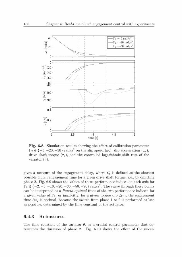
158 Chapter 6. Real-time clutch engagement control with experiments
ωs
[rad
/s]
0
20
40
ωs
[rad
/s2]
−80
−60
−40
−20
0
τ d[N
m]
0
200
400
600
ν[1
/s]
time [s]3 3.5 4 4.5 5
0
0.2
0.4
Γ2 =-5 rad/s2
Γ2 =-20 rad/s2
Γ2 =-50 rad/s2
Fig. 6.8. Simulation results showing the effect of calibration parameterΓ2 ∈ −5,−20,−50 rad/s2 on the slip speed (ωs), slip acceleration (ωs),drive shaft torque (τd), and the controlled logarithmic shift rate of thevariator (ν).
gives a measure of the engagement delay, where t∗2 is defined as the shortestpossible clutch engagement time for a given drive shaft torque, i.e., by omittingphase 2. Fig. 6.9 shows the values of these performance indices on each axis forΓ2 ∈ −2,−5,−10,−20,−30,−50,−70 rad/s2. The curve through these pointscan be interpreted as a Pareto-optimal front of the two performance indices: fora given value of Γ2, or implicitly, for a given torque dip ∆τd, the engagementtime ∆t2 is optimal, because the switch from phase 1 to 2 is performed as lateas possible, determined by the time constant of the actuator.
6.4.3 Robustness
The time constant of the variator θv is a crucial control parameter that de-termines the duration of phase 2. Fig. 6.10 shows the effect of the uncer-

6.4 Simulations 159
Δτd/τd [-]
Δt 2
/t∗ 2
[-]
0 0.2 0.4 0.6 0.8 10
0.1
0.2
0.3Γ2 = −2 rad/s2
Γ2 = −20 rad/s2
Γ2 = −70 rad/s2
Fig. 6.9. Simulation results showing the effect of the calibration parame-ter Γ2 ∈ −2,−5,−10,−20,−30,−50,−70 rad/s2 on the relative torquedip (∆τd/τd) and the relative engagement delay (∆t2/t
∗2). Lower values
correspond to better performance.
Γ2 [rad/s2]
ln(θ
v/θ
v)
[-]
0.6
0.4
0.2
−60 −40 −20
−0.6
−0.4
−0.2
0
0.2
0.4
0.6
Δτd/τd [-]
Γ2 [rad/s2]
0.02 0.06 0.2
−60 −40 −20
Δt2/t∗2 [-]
Fig. 6.10. Simulation results showing the effect of a mismatch in thevariator time constant θv on the relative torque dip (left) and the relativeengagement delay (right), as a function of the calibration parameter Γ2.
tainty in this time constant for the driving situation. The relative performanceindices ∆τd/τd and ∆t2/t
∗2 are evaluated for various values of the estimated
time constant θv/θv ∈ [0.5, 2] and various values of the calibration parameterΓ2 ∈ [−70,−2] rad/s2. As expected, an underestimated time constant (i.e.,
ln(θv/θv) < 0) has a large influence on the smoothness of the clutch engagement∆τd, but only a small influence on the engagement time ∆t2. An overestimatedtime constant on the other hand (i.e., ln(θv/θv) > 0) has a large influence onthe engagement time, but only a small influence on the smoothness of the clutchengagement. This result confirms the reasoning in Section 6.3.7, that it is nec-essary to choose a large estimate of θv to meet the smoothness criterion, but atthe cost of a conservative clutch engagement time.

160 Chapter 6. Real-time clutch engagement control with experiments
6.5 Experiments
Experiments are performed on a mechanical hybrid powertrain, mounted on atest rig, to validate the control performance and its robustness against realisticsensor noise and modeling uncertainties. A set of experiments that is similarto the simulations are performed on a scaled test rig, to answer two researchquestions: i) How does the controller perform in the flywheel driving mode?ii) What is the effect of calibration parameter Γ2 on the clutch engagementperformance? Before giving answers to these research questions, a descriptionof the experimental setup is given.
6.5.1 Test rig
The test rig, shown in Fig. 6.11, consists of an electric machine in series witha flywheel, CVT with integrated clutch and variator, drive shaft, and anotherelectric machine. Two sensor shafts are mounted on each side of the CVT tomeasure the torques and rotational speeds for diagnostic purposes, i.e., thesesignals are not used by the controllers. The electric machine mounted on theflywheel side is used to accelerate the flywheel to its initial rotational speed andis switched off afterwards. For practical reasons, the compact vacuum-housedflywheel of the driveline in Fig. 6.1 is replaced by the engine flywheel of a truck,without any gear reduction. Consequently, the drag losses are higher, whereasthe inertia acting on the clutch (flywheel + electric machine) is about 50% ofthe reference flywheel.
The mass-produced CVT has an integrated wet friction clutch, a variator, anda final drive. The clutch and variator are hydraulically actuated, fed by theintegrated pump that is located on the flywheel side of the clutch. In orderto generate sufficient hydraulic actuation power, the flywheel must rotate at aminimum speed of 100 rad/s, so the braking situation where the flywheel is ac-celerated from standstill cannot be performed using this test rig. This problemneeds to be circumvented, e.g., using a hydraulic accumulator, before the systemcan be implemented in a vehicle. The controllers for the clutch and variator arestandard component controllers, cf. the descriptions in Sections 6.2.2 and 6.2.3,which are implemented on the hardware provided by the manufacturer. Thesecontrollers are set to track the setpoints created by the clutch engagement con-troller, which are externally provided using the Controller Area Network (CAN)interface. The required sensor signals from the CVT are acquired using the sameinterface.
The single drive shaft represents the stiffness of approximately 50% of the twodrive shafts shafts in the reference vehicle. The electric machine mounted onthe drive shaft is used to mimic the load torque and the inertia of the vehicle

6.5 Experiments 161
torque & speed sensor
continuously variable transmission drive shaft
electric machine
electric machine flywheel
torque & speed sensor
integrated wet friction clutch
Fig. 6.11. Overview of the experimental setup, which shows the flywheel,the CVT, the drive shaft, the sensor shafts, and the electric machines.
using a feedback controller and the load torque. The “virtual” vehicle inertia isused as a parameter to match the resonance frequency of the test rig with thatof the mechanical hybrid reference vehicle (i.e., 1.3 Hz for rv = rv). Since theflywheel inertia and drive shaft stiffness are about 50% of those in the referencevehicle, the vehicle inertia is scaled to approximately 50% of that of the referencevehicle. The feedback controlled system for the vehicle inertia has a cross-overfrequency of approximately 6 Hz with a small phase margin, so i) the controlloop may not be sufficiently fast to accurately reproduce the 1.3 Hz resonanceof the drive shaft and ii) oscillations of 6-8 Hz are easily excited and present inthe measured signals. Nevertheless, this experimental setup is still suitable tovalidate the controller design and its robustness against measurement noise andmodeling errors.
6.5.2 Control performance
The control performance for the driving situation is shown in Fig. 6.12, usingthe parameters as listed in Table 6.2. As expected, similar results are obtainedas with the simulation, showing a fast reduction of the slip speed ωs in phase 1,and a smooth reduction of the slip acceleration ωs in phase 2. The speed ratiorv and drive shaft torque τd are quite noisy shortly after starting up when theresonance of the test rig is excited. The drive shaft torque remains quite closeto the demanded 200 Nm in phases 1 and 2, and slightly drifts away in phase3, caused by the feedforward controller (6.36) in phase 3 that completely relieson the relatively simple modeling of the variator dynamics (6.3). On the otherhand, this simple model has proven to be effective to achieve the desired slipacceleration value of Γ2 = −20 rad/s2 quite accurately, so that the resultingdrive shaft torque is hardly disturbed by the clutch engagement. Experimentson a cold transmission (30 C) give similar results (not shown here) as for thewarm transmission (60 C) shown in Fig. 6.12, which gives an indication of therobustness against different operating conditions. Overall, the experiment shows

162 Chapter 6. Real-time clutch engagement control with experiments
a good control performance and robustness against realistic modeling errors andmeasurement noise.
6.5.3 Calibration parameter
The effect of the calibration parameter Γ2 on the clutch engagement is evalu-ated for two values, which have shown in the simulations an acceptable torquedip (Γ2 = −20 rad/s2) and a relatively large torque dip (Γ2 = −50 rad/s2).The results in Fig. 6.13 show that the desired slip accelerations at the timeof clutch engagement are achieved quite accurately, resulting in different driveshaft torques: the slip acceleration of Γ2 = −20 rad/s2 results in a negligibletorque dip, whereas the slip acceleration of Γ2 = −50 rad/s2 results in an un-comfortable relative torque dip of 35%, after which the shift rate of the variator(ν) slowly recovers. The torque dip is smaller and less oscillatory than in thesimulations, which can be explained by the different damping characteristics ofthe drive shaft, the higher viscous friction in the flywheel, and the limited band-width of the vehicle inertia controller on the test rig. The resulting torque offsetsare acceptable, yet there is room for improvement, e.g., by including a feedbackcontrol loop for the drive shaft torque based on a torque observer. Overall, Γ2
shows to be an effective calibration parameter to determine the trade-off betweenclutch engagement time and the torque dip size.
6.6 Conclusions
The control problem of fast and smooth clutch engagement is considered fora mechanical hybrid powertrain that uses a flywheel system for kinetic energystorage and a CVT for power transmission. This chapter contributes with a new,simple and robust controller design with a consistent performance under differentinitial conditions. The controller is based on the relevant actuator dynamicsand the clutch slip dynamics. The clutch slip dynamics is controlled using thestandard speed sensors such that the desired slip acceleration is achieved atthe time of clutch engagement. The desired slip acceleration is useful as thecalibration parameter to choose the trade-off between fast and smooth clutchengagement. Simulations show that the generic controller is effective for thedriving and braking situation. A parameter variation study is performed toillustrate how the calibration parameter and the uncertainty in the variatortime constant influence the clutch engagement performance. For uncertain timeconstants of the actuator, smooth clutch engagement can still be achieved, but atthe cost of a conservative clutch engagement time. Test rig experiments validatethe effectiveness of this relatively simple controller and its robustness againstrealistic modeling errors and measurement noise.

6.6 Conclusions 163
ω[r
ad/s
]
0
100
200ωfωp
ωd/rd
ωs
[rad
/s]
0
50
100 ωs
Ω1Ω2
ωs
[rad
/s2]
−60−40−20
0
ωs¯ωs
τ c[N
m]
0
20
40 τc
τ ′c
ν[1
/s]
0
0.2
0.4
νν ′
r v[-]
0.5
1
1.5
time [s]
τ d[N
m]
0 1 2 3 4 5 6 7 80
100
200
300
τdτd
t0t1
t2
phase 1 phase 2 phase 3
Fig. 6.12. Experimental results for the driving situation. The slip accel-eration at clutch engagement matches the desired value Γ2 ≈ −20 rad/s2
sufficiently accurately, resulting in a fast and smooth clutch engagementthat hardly disturbs the drive shaft torque.

164 Chapter 6. Real-time clutch engagement control with experiments
ωs
[rad
/s]
0
20
40
ωs
[rad
/s2]
−80
−60
−40
−20
0
20
τ d[N
m]
100
150
200
250
ν[N
m]
time [s]4.5 5 5.5 6
0
0.2
0.4
Γ2 = −20 rad/s2
Γ2 = −50 rad/s2
Fig. 6.13. Experimental results for two calibration parameter values.The torque dip (τd) increases significantly when decreasing the calibrationparameter Γ2 from −20 rad/s2 to −50 rad/s2.

Chapter 7
Conclusions andrecommendations
7.1 Conclusions
This thesis has presented an integral design approach for the optimization ofi) the hybrid powertrain topology and flywheel size, ii) the energy controllerthat is suitable for implementation in real-time hardware, and iii) the torquecontroller, which is validated with test bench experiments. In Part I, optimalcontrol has formed the basis for the optimization of the hybrid powertrain andenergy controller. In Part II, real-time control has formed the basis for thedesign of the energy controller and torque controller. For the energy controller,the unavoidable discrepancy between optimal and real-time control is bridged byi) reduction of the optimization problem to the essential control and state space,ii) prediction of future driving conditions based on statistics, and iii) extractionof intuitive rules from the explicit optimal controller. The main results andconclusions are further discussed below.
7.1.1 Hybrid powertrain design
Chapter 2 has optimized the topology and the flywheel size of a mechanicalhybrid powertrain, from an extensive set of over twenty different concepts de-scribed in the literature. The competitiveness of each powertrain is evaluatedbased on the fuel saving potential and the cost of hybridization with respect toa conventional powertrain equipped with an Automated Manual Transmission(AMT). The hybrid powertrains are composed of realistic component models,based on experimental data as described for the Continuously Variable Trans-mission (CVT) and flywheel system in Appendix A. The optimal fuel saving is

166 Chapter 7. Conclusions and recommendations
computed for a limited set of flywheel sizes and driving cycles, using the numer-ical optimization method as described in Appendix B. Results show that threeof the considered topologies have a very competitive ratio between the fuel sav-ing and hybridization cost, which can be quantified by a relative payback period1
between 39%−45% of the service life (150, 000 km) of passenger vehicles. Whenconsidering also other criteria, such as control complexity, clutch wear, and driv-ing comfort, the mecHybrid topology described in [4] is expected to be the mostcompetitive. The associated optimal energy storage capacity of the flywheel isequivalent to the kinetic energy of the vehicle during urban driving (50 km/h),which is one of the key functionalities of mechanical hybrid powertrains. Due tothe relatively small differences between the investigated topologies, however, itis concluded that mechanical hybrid powertrains in general have the potentialto be economically attractive. This is especially the case for the CVT-basedhybrid powertrains, which also improve the driving comfort with respect to theAMT-based conventional powertrain.
7.1.2 Energy controller design
Chapter 3 has presented a detailed powertrain model for the optimized hybridpowertrain design of Chapter 2. Constraints on the control space are definedin order to avoid driving mode switches that are expected to be uncomfortable.This model is used to find the optimal sequence of driving modes and powersplits between the engine and flywheel system, that minimizes the overall fuelconsumption for a pre-defined driving cycle. This relatively complex optimiza-tion problem is solved for six representative driving cycles using dynamic pro-gramming. Results show that, despite the relatively low energy storage capacityof the flywheel, very high fuel savings can be obtained of between 20% − 40%,similar to that of (costly) electric hybrid powertrains [148]. Analysis of the re-sults shows that each fuel saving functionalities, which are i) recuperation ofbrake energy for later use, ii) elimination of inefficient part-load operation ofthe engine, and iii) engine shut-off during vehicle standstill, contributes witha significant amount to the fuel saving potential, although a part of the fuelsaving potential is canceled by the increased power dissipation in the transmis-sion. The power dissipation is partly increased due to a more frequent usage,i.e., also during brake energy recuperation, and partly due the higher rotationalspeeds of the transmission components. Nevertheless, additional cooling is notexpected to be necessary, since the higher power dissipation mainly occurs dur-ing low-power urban driving, while it is well distributed over time and amongthe different components. The design problem for the energy controller can besubstantially reduced by considering only two power split values, instead of aquantized range, with a negligible impact on the fuel saving potential (difference
1Relative payback period [%] = 100 [%] × hybridization cost [€]/(fuel saving [l/km] × fuelprice [€/l] × service life [km])

7.1 Conclusions 167
< 0.4%) and the optimal energy controller. This result is an important steptowards the design of the real-time controller in Chapter 5.
Chapter 4 has presented an extension to the powertrain model described inChapter 3, by describing the thermodynamic powertrain heating and the influ-ence of the powertrain temperature on the frictional power dissipation in theengine and transmission. The impact of cold start conditions, referring to a coldpowertrain temperature (20 C) and a stationary flywheel system, are investi-gated on the fuel saving potential and optimal energy controller. Results showthat the impact of the low powertrain temperature on the absolute fuel consump-tion is almost independent of the driving cycle, and is well approximated by asimplified model. The impact is higher for the hybrid powertrain than for theconventional powertrain due to a lower “heating efficiency”, which is inherentto the higher mechanical efficiency. The impact of the cold start conditions onthe fuel saving potential, however, is significant (4.0%-7.3%) with respect to thewarm start conditions as described in Chapter 3. The optimal energy controller,however, is hardly affected by the cold powertrain temperature, as it aims atmaximizing the average mechanical efficiency of the engine independent of thepowertrain temperature. Based on this insight, the temperature state can beeliminated from the state space for the real-time controller design in Chapter 5.
Chapter 5 has presented the design of a real-time energy controller for the re-duced optimization problem that follows from Chapters 3 and 4. A genericdesign framework is followed starting with an optimal controller, converting itto a causal controller, and make it robust afterwards. For the considered me-chanical hybrid powertrain, the optimization problem is solved using dynamicprogramming. The future driving conditions are modeled by a smooth approx-imation of statistical data, and implemented in the receding model predictivecontrol framework. The controller is made tunable by rule extraction based onphysical understanding of the system, which gives insights in the implicit decisionprocess of the numerical optimization. Using the gained insights, the hysteresisband that damps the switches between flywheel driving and hybrid driving, isassigned as the single calibration parameter to increase the robustness againstprediction uncertainties. Results show that due to the unavoidable predictionuncertainty, the fuel saving potential with the real-time controller is a signifi-cantly (2.1%-7.8%) lower than with the optimal controller, yet a transparant,causal, and tunable controller is obtained. The remaining fuel saving potential isstill high under warm start conditions (16.8%−29.1%) and significant under coldstart conditions (12.6%− 22.8%). The followed numerical approach is not onlysuitable for this mechanical hybrid powertrain, yet for an entire class of emerginghybrid powertrains that use multiple driving modes to combine the benefits ofseveral components in a complex topology (i.e., with switched dynamics) usingdownsized components to reduce cost (i.e., with active state constraints).

168 Chapter 7. Conclusions and recommendations
fuel
consu
mption
[%]
NEDC WLTP FTP75 EHV JC08 CADC−40
−30
−20
−10
0
optimal, warm startoptimal, cold startreal-time, cold start
Fig. 7.1. Degradation of the fuel saving potential towards more realistic(cold start) driving conditions and (real-time) controller design for thecertified driving cycles (NEDC, FTP75, and JC08) and (parts of) real-world driving behavior measured in worldwide industrialized countries(WLTP, [79]), Europe (CADC, [80]), and Eindhoven (EHV, the Nether-lands).
Following the optimal controller results under warm start conditions in Chap-ter 3, to the cold start conditions in Chapter 4, and the real-time controllerresults in Chapter 5, a gradual degradation can be observed in the fuel savingpotential, as summarized in Fig. 7.1. Such a performance degradation is unavoid-able when adding realistic features to a complex system, which has to be robustagainst versatile user and external conditions. On the other hand, this thesishas considered three major impacts that are often neglected in the literature,which are i) constraints to avoid uncomfortable dynamics in Chapter 3, ii) coldstart conditions in Chapter 4, and iii) prediction without (costly) navigation orradar telemetry systems in Chapter 5. Also, realistic power dissipation modelshave been used, which are based on dedicated test rig experiments for the CVTand flywheel system as described in Appendix A and for the internal combus-tion engine in Chapter 4. Despite the possible further degradation of the fuelsaving potential after in-vehicle implementation, this mechanical hybrid power-train design is expected to be still very promising. Especially for the (sportive)urban driving cycles (EHV, JC08 and CADC), the fuel saving potential is stillvery high, ranging between 19.5% and 22.8% for the cold start conditions andbetween 23.1% and 29.1% for the warm start conditions.
The fuel saving potential with the real-time controller can be put into perspec-tive when considering the relative payback period, using the approach describedin Chapter 2. Here, the conventional CVT-based powertrain is selected as thereference cf. Chapters 3-5, in contrast to the less comfortable AMT-based pow-
7.2 Recommendations 169
ertrain in Chapter 2. The results show that the relative payback period foradding the flywheel system and some minor adaptation is returned after already17%− 43% of its service life, which is better than the results reported in Chap-ter 2 due to the different reference powertrain and a wider selection of drivingcycles. The relative payback period becomes even more attractive when antici-pating increasing fuel prices [1] and longer utilization of passenger vehicles thanthe service life for passenger vehicles of 150,000 km.
7.1.3 Torque controller design
Chapter 6 has presented a new systematic design framework for a (real-time)torque controller, with the focus on the critical trade-off between fast and smoothclutch engagement. The resulting controller is based on the relevant actuatordynamics and the clutch slip dynamics. The clutch slip dynamics is controlled us-ing the standard speed sensors such that the desired slip acceleration is achievedat the time of clutch engagement. The desired slip acceleration is useful as thecalibration parameter to choose the trade-off between fast and smooth clutchengagement. Simulations show that the generic controller is effective for thedriving and braking situation. A parameter variation study is performed to il-lustrate how the calibration parameter and the uncertainty in the variator timeconstant influence the clutch engagement performance. For uncertain time con-stants of the actuator, smooth clutch engagement can still be achieved, but atthe cost of a conservative clutch engagement time. Test rig experiments validatethe effectiveness of this relatively simple controller and its robustness againstrealistic modeling errors and measurement noise.
7.2 Recommendations
The integral design optimization as presented in this thesis can be extendedby considering additional relevant aspects. Moreover, the presented real-timecontrollers are suitable for implementation and calibration, yet need some ex-tensions before they can be validated in a prototype vehicle. Several researchdirections regarding these extensions are outlined below.
7.2.1 Design optimization
The design of a competitive hybrid powertrain must consider many differentand sometimes conflicting marketing and production objectives, as argued inChapter 2. For the design of the optimal energy controller in Chapters 3-4,the fuel consumption has been selected as the single optimization objective,whereas comfort requirements are considered with state-dependent constraintson the control space. This approach offers a clear distinction between the pri-mary objective (fuel consumption) and the secondary objective (comfort), which

170 Chapter 7. Conclusions and recommendations
are only occasionally in conflict with each other. Consequently, the conflictingsituations can be avoided by the constraints on the control space. The result-ing optimization problem is therefore distinct, as the optimal solution is clearlydefined. Following this approach, the energy controller can also be extended,by minimizing the emission of pollutants and greenhouse gases as a secondaryobjective, which is only occasionally in conflict with the fuel consumption, i.e.,under dynamic engine operating conditions [149].
Similarly, the control of the hydrodynamics can be added as a secondary objec-tive. The relevant hydrodynamics for the energy controller are the i) filling ofthe hydraulic accumulator, which provides hydraulic pressure when the pumpis stationary, and the ii) filling of the clutch chambers, which determines theresponse time of the clutch. Under normal driving conditions, the excess hy-draulic power generated by the pump can be used to fill the accumulator andclutches, and is therefore not in conflict with the fuel consumption. However,occasionally, the hydraulic power generation becomes insufficient, so the controlspace of the energy controller must be constrained to increase the pump speed,i.e., to increase the hydraulic power.
The distinction between primary and secondary objectives is not possible whenthe objectives are generally in conflict (i.e., not occasionally), such as the hy-bridization cost and fuel saving potential in Chapter 2. Then, the objectivesmay be combined in a mixed cost function, which is only sensible when theperformance indices are somehow comparable, such as the cost/benefit ratio ex-pressed by the relative payback period in Chapter 2. If the objectives are notcomparable, as with the (subjective) comfort requirements, no unique optimumcan be defined. Instead, a Pareto-optimal front can be found, which describes afamily of optimal solutions for different trade-offs between the objectives, suchas with the fast and smooth clutch engagement controller described in Chap-ter 6. The “optimal” trade-off must then be tuned by an experienced calibrationengineer. Following this approach, the constant brake power split between theflywheel system and disc brakes, as described in Chapter 3, can be extended toa dynamic control strategy. The subjective trade-off is then to maximize brakeenergy recuperation, while minimizing the inconsistency of the brake pedal re-sponse, e.g., caused by energy storage limits and driving mode switches.
An extension to the design optimization of the mechanical hybrid powertrain isto add a boosting2 functionality using the same flywheel system. Such an exten-sion probably leads to a higher hybridization cost and a higher fuel consumptiondue to higher transmission losses, resulting in a subjective trade-off between ac-celeration performance, cost, and fuel saving. Alternatively, a compact electric
2The term “boosting” refers to a functionality of the flywheel system to assist the internalcombustion engine in order to improve the acceleration performance of the vehicle [46].

7.2 Recommendations 171
power source can be added to combine the favorable power capacity of the fly-wheel system with the favorable energy storage capacity of the batteries, andthe favorable controllability of the electric machine. Adding these design dimen-sions, however, substantially complicates the integral design optimization of thehybrid powertrain.
7.2.2 Real-time controller validation
A prototype vehicle is currently under development3 with the aim to demon-strate the fuel saving potential of the considered mechanical hybrid powertrain.The real-time controllers presented in Chapters 5 and 6 are suitable for in-vehicleimplementation and calibration, yet require some extensions for actual on-roadvalidation. Chapter 5 has presented the energy controller based on statisticsof existing driving cycles, in order to predict future driving conditions. Likemost (certified) driving cycles, however, the selected driving cycles only considervariations in the vehicle velocity, while neglecting relevant variations in road al-titude. These variations in road altitude, as well as other variations (e.g., wind,road surface quality), can be included using the same design framework, by in-troducing a third driving cycle state for the power demand (besides velocity andacceleration), thereby separating the vehicle velocity prediction from the powerdemand prediction.
Chapter 6 presented the torque controller for the flywheel driving mode dur-ing the critical clutch engagement phase. This controller can be extended toother driving modes when considering the engine as the actuator instead of theCVT, as elaborated for a dual clutch transmission in [138]. Switches betweendriving modes have not been elaborated in this thesis, yet only described inChapter 3. Three switch types can be distinguished. The “disengaging switch”from hybrid driving to another driving mode is expected to give no problems,as the clutch needs only to be disengaged. The “engine cranking switch” fromflywheel driving to another driving mode may cause an uncomfortable torquedip, as torque is required to crank the engine while the flywheel system propelsthe vehicle. This problem can be avoided by controlling the slip in the transmis-sion clutch during cranking, and engaging the clutch afterwards using the clutchengagement controller as described in Chapter 6. The difficult “synchronizationswitch”, from engine driving to another driving mode during vehicle propulsion,has been circumvented as described in Chapter 3, due to the expected comfortissues. During vehicle braking, however, this switch is supported as the discbrakes provide the braking torque. Then, after disengagement of the engine andengagement of the flywheel system, the transmission clutch can be engaged us-
3The demonstrator vehicle is part of the “mecHybrid” project, which is a research projectof a consortium between academic and industrial partners (i.e., see acknowledgments on theback of the title page).

172 Chapter 7. Conclusions and recommendations
ing the clutch engagement controller. Meanwhile, the earlier mentioned brakepower split strategy must provide an “optimal” trade-off between brake energyrecuperation and consistency of the brake pedal response.

Appendix A
Semi-empirical power dissipationmodeling
Abstract – Accurate modeling is of key importance for the model-based design of controlled
systems. Often, relatively simple component models are sufficient to capture the main charac-
teristics, thereby keeping the overall system complexity limited. For each component model,
smooth characteristics are preferred, such that unnecessary irregularities can be avoided in the
design optimization and in the controlled signals. This chapter presents the design of such
control-oriented models to describe the power dissipation in the key mechanical hybrid power-
train components, i.e., the Continuously Variable Transmission (CVT) and flywheel system.
The power dissipation in these components are modeled by parametric functions, which are
suitable to describe smooth characteristics in a relatively simple format with only a few coef-
ficients. The functions are selected based on physical understanding of the systems, whereas
the coefficients are identified from dedicated test rig experiments. Results show that the power
dissipations are modeled very accurately for both the CVT and the FS, with a modeling error
of less than 75 W for 80% of the operating conditions in a wide operating range between
−25 kW and 38 kW. The CVT model is also validated under dynamic driving conditions,
showing an overall error for the power transmission efficiency of less than 1%.
A.1 Introduction
In the past decades, automotive powertrains have become increasingly complexin order to meet stringent requirements regarding fuel economy, emissions, anddriving comfort. One example is the hybrid powertrain, which adds a secondarypower source to the internal combustion engine in order to improve the overallfuel economy and emissions. The hybrid powertrain can be seen as a controlledsystem that is composed of several components, which in their turn, are con-

174 Appendix A. Semi-empirical power dissipation modeling
trolled systems on a sub-system level. Since the overall performance cannot becharacterized independently from the controller and the selected components,an integral design approach is needed [22], which is often based on optimal con-trol [35, 39,120].
The use of optimal control asks for control-oriented models, which capture onlythe “input-output” characteristics on a system level, thereby taking sub-systemdetails implicitly into account. The model must be accurate in order to fullyexploit the potential of the controlled system, and smooth to avoid irregularitiesin the design optimization results and unnecessary variations in the controlledsignals. Often, relatively simple component models are sufficient to capture themain characteristics, thereby keeping the overall system complexity limited, suit-able for extensive parameter variation studies for the design optimization, andfor limited computational resources in real-time hardware.
The modeling methods can be divided in three classes, which are the i) firstprinciple, ii) empirical, and iii) semi-empirical classes. The first principle classis entirely based on theory, such as Newton’s law of motion, which is suitable tomodel the dynamics in the powertrain, in the form of differential equations [150].This class is less suitable to model complex interactions, such as friction-basedpower dissipation, in a simple format. The empirical class, which is entirelybased on experiments, on the other hand, is suitable to model power dissi-pation characteristics in the form of look-up tables [63]. The measured datausually requires some postprocessing to filter irregularities caused by measure-ment uncertainties, and to extrapolate measurements to parameter spaces thatare not covered by the measurement due to limitations of the test equipment.Systematic postprocessing, however, using well-motivated assumptions for thefiltering and extrapolation is a challenging task, especially when dealing with amulti-dimensional parameter space. The semi-empirical class overcomes theseproblems by choosing a modeling framework based on physical understandings,while using experiments to identify the finite number of coefficients. This classcombines the simplicity of the first principle class, with the ability to capturerealistic characteristics of the empirical class. Examples of semi-empirical powerdissipation models are piecewise affine and quadratic approximations for inter-nal combustion engines [26, 114], piecewise affine approximations for electricmachines [151, 152], parametric approximations for gears [153], and parametricapproximations for flywheel systems [5, 7, 10].
A.1.1 Mechanical hybrid powertrain components
This research work considers the mechanical hybrid powertrain as schematicallydepicted in Fig. A.1. The main powertrain components are the internal combus-tion engine for mechanical power generation, the Continuously Variable Trans-

A.1 Introduction 175
engine
CVT
rotor
flywheel system
wheels
gears
clutches
(a) Schematic representation of the mechanical hybrid pow-ertrain topology.
flywheel system
CVT
(b) 3D representation of theCVT and FS.
Fig. A.1. The mechanical hybrid powertrain uses a CVT to propel thevehicle using kinetic energy of the FS and to recuperate kinetic energy ofthe vehicle to energize the FS.
mission (CVT) for mechanical power transmission, and the Flywheel System(FS) for short-term kinetic energy storage. The FS is mechanically connectedby the CVT, which allows for efficient power transmission by continuously chang-ing its speed ratio, in order to propel or brake the vehicle. The fuel economybenefits can be attributed to i) recuperation of brake energy using the FS; ii)elimination of inefficient part-load operation of the engine, by driving purely onthe FS with the engine shut-off, or by energizing the FS while propelling the ve-hicle at fuel-efficient operating points of the engine; and iii) engine shutoff duringvehicle standstill [66]. In order to fully exploit the fuel saving functionalities,a powertrain controller is needed that coordinates the components in order tominimize the overall fuel consumption for given driving conditions. The designof such a controller requires control-oriented models that describe the power dis-sipation of the components. The distinguishing components of this mechanicalhybrid powertrain are the CVT and FS, which are operated in both power di-rections, i.e., for vehicle propulsion and regenerative braking. The consideredCVT is a conventional, mass-produced unit [9], for which the control is modifiedto enable regenerative braking [64]. The considered FS is a prototype, compactunit especially developed for this mechanical hybrid powertrain concept [4].
The power dissipation in CVTs and FSs is widely studied in the literature inorder to improve the design on component level (i.e., CVT and FS), yet has notresulted in the desired semi-empirical models to improve the design on power-train level. For CVTs, the power dissipation has been experimentally quanti-fied for one power direction (i.e., propulsion) [154, 155] to understand its im-pact on the fuel economy of conventional (non-hybrid) vehicles [156, 157]. The

176 Appendix A. Semi-empirical power dissipation modeling
power dissipation has been decomposed into different mechanisms [158–162] togain insights to improve the CVT design [34, 163, 164] and the controller de-sign [145,165–167]. Extensive overviews regarding these developments are givenin [9,168,169]. Similarly, for FSs, the power dissipation has been experimentallyquantified and decomposed [10] in order to improve its design in [5, 7] and tounderstand its impact on the fuel economy of flywheel-assisted vehicles [11,47].
A.1.2 Main contribution and outline
This chapter contributes with semi-empirical models for the power dissipationin the CVT and FS, which are based on the physical understanding of the mainpower dissipation mechanisms described in the literature. The power dissipationcharacteristics are modeled using parametric functions, which are suitable todescribe smooth characteristics with only a few coefficients. The coefficients,which are specific for the considered CVT and FS, are identified with variousexperiments on two dedicated test rigs. For the CVT, the power dissipationis identified under static operating conditions, and validated under dynamicoperating conditions prescribed by two certified driving cycles. For the FS, twotypes of operating conditions considered, which are i) the unloaded conditions toidentify the energy storage efficiency of the rotor, and ii) the loaded conditionsto identify the power transmission efficiency of the gear set. In summary, themain contributions are
• semi-empirical power dissipation models for a conventional CVT and aprototype FS; and
• accurate experimental results for both systems in both power directions,i.e., for vehicle propulsion and regenerative braking.
The outline is given as follows: Section A.2 describes the power dissipationexperiments for the CVT and the FS. Section A.3 describes the design of thesemi-empirical models, of which their accuracies are evaluated in Section A.4.Section A.5 summarizes the main conclusions.
A.2 Experiments
A set of experiments is designed to accurately measure the power dissipation inthe CVT and the FS, under realistic driving conditions. In the sequel, first eachsystem is described in more detail, followed by descriptions of the dedicated testrigs, the controller setpoints, and some qualitative results.

A.2 Experiments 177
ωp
τp
ωs τs
section A-A A
A
Fp
Fs
Rp
Rs
Fig. A.2. Schematic representation of the variator, which consists of apushbelt clamped between the primary and secondary pulley pairs
.
A.2.1 System description
A.2.1.1 CVT
The conventional, mass-produced CVT originates from a compact passengervehicle and has a torque capacity of 140 Nm. The system has an integratedhydraulic pump, torque converter, Drive / Neutral / Reverse (DNR), pushbelt-driven variator, final drive, differential, and a cooling circuit. The key componentof the CVT is the variator, which consists of a metal pushbelt clamped betweentwo pulley pairs on each side of the variator as shown in Figure A.2, also referredto as the primary (subscript “p”) and the secondary (subscript “s”) ides. Eachpulley pair consists of one axially fixed sheave and one axially moveable sheave,on which an axial force (F can be generated by an oil pressure, which is con-trolled by a hydraulic system and fed by the pump. The clamping forces enabletorque transmission (τ) through the pushbelt, by means of friction. The levels ofthe clamping forces (Fp and Fs) determine the maximum transmittable torque,whereas the ratio between the clamping forces determines the ratio rv := ωs/ωp
between the rotational speeds (ω).
A.2.1.2 FS
The prototype FS is developed for the mechanical hybrid powertrain conceptwith the focus on safety, low power dissipation, and low manufacturing cost,subject to noise and durability constraints [4]. The system contains a steel rotorplaced in a mild vacuum (100 mbar) that is connected with a two-stage gear setto operate the rotor (subscript “r”) at a relatively high rotational speed (up to3140 rad/s). The rotational speed of the flywheel system shaft (subscript “f”)operates close to the engine speed range (between 105 rad/s and 262 rad/s) under

178 Appendix A. Semi-empirical power dissipation modeling
ωf τf
ωr gear angle
A
A
section A-A
Fig. A.3. Schematic representations of the FS, which consists of a two-stage gear set and a rotor, which can be separated by the clutch indicatedin grey.
normal urban driving conditions, thereby facilitating a combined operation ofthe FS and engine. When the FS is coasting, the rotor can be disengaged fromthe gear set using a compact clutch.
A.2.2 Test rig
A.2.2.1 CVT
The CVT is mounted between two sensor shafts and two electric machines asshown in Figure A.4. For the considered experiments, the DNR is put in “Drive”position, and the differential is locked to connect with electric machine 2. Duringvehicle standstill, the DNR cannot be put automatically in “Neutral” position,resulting in a unrealistic situation with a relatively high power dissipation dueto the slipping torque converter. The power dissipation of a slipping torque con-verter, however, is not relevant for the considered mechanical hybrid powertrain,as it uses a clutch instead (see, Figure A.1(a)). The cooling circuit is connectedwith an external pump to a (cold) water reservoir, in order to control the lubrica-tion oil temperature around its operating temperature between 75 C and 80 C.The original transmission control unit is replaced by an external controller to en-able flexible operating points, i.e., that are not fixed by the variogram. For thiscontroller, a conventional speed ratio strategy is adopted for accurate trackingof the desired speed ratio, as described in [170]. A conventional (safe) clampingstrategy is adopted and extended for reversed power flows to enable regenerativebraking, as described in [64]. The torque converter is controlled such that it locksautomatically once the slip speed reaches a certain threshold (< 10 rad/s). Thetwo sensor shafts use strain gauges and optical encoders to measure the torqueand speed on both the primary (sensor shaft 1) and the wheel (sensor shaft 2)

A.2 Experiments 179
electric machine 1 continuously variable transmission electric machine 2
sensor shaft 1 sensor shaft 2
Fig. A.4. Test rig for the mass-produced pushbelt CVT, which is con-nected to two electric machines that mimic realistic operating conditions,and sensors shafts in between to measure the torque and rotational speed.
shafts of the CVT. The torque capacities of the sensors are selected to be suffi-cient for most relevant driving conditions, but limited to keep the proportionallyrelated sensor noise low. As a trade-off, a torque capacity of 200 Nm is selectedfor the primary shaft and 500 Nm for the output shaft. This selection coversthe torque ranges for a compact 1110-kg passenger vehicle equipped with a 1.5-lgasoline internal combustion engine, under normal driving conditions prescribedby most certified driving cycles that have no variations in altitude. The electricmachines are controlled by a power electronics unit, which can accurately trackthe torque or speed setpoints. The overall test rig is operated with setpoints forthe speed of electric machine 1, the torque of electric machine 2, and the speedratio of the CVT.
A.2.2.2 FS
The FS is connected to a sensor shaft and an electric machine as shown inFig. A.5. Here, the same sensor shaft as on the primary side of the CVT is used.The rotor can be (de-)energized by applying a torque on the external shaft whenthe clutch is engaged. The clutch can be (dis-)engaged by applying a pressure onthe clutch plates, which is hydraulically controlled by a two-port switch valve.On the rotor-side of the clutch, a speed sensor is integrated to monitor therotor speed. The lubrication oil of the gear set is pre-heated to its operatingtemperature of 65 C by an external heater before the experiments. The overalltest rig is operated with setpoints for the torque of the electric machine and thevalve position of the FS.

180 Appendix A. Semi-empirical power dissipation modeling
flywheel system electric machine
sensor shaft
Fig. A.5. Test rig for the prototype FS, which is connected to an electricmachine and a sensor shaft.
A.2.3 Controller setpoints
A.2.3.1 CVT
For the CVT, two types of operating conditions are selected: i) static conditionsfor a wide operating range, and ii) dynamic conditions for two certified drivingcycles, i.e., the New European Driving Cycle (NEDC) and the Japanese 10-15mode (JP1015). For the static experiments, static operating points are selectedfor the primary torque τp, primary speed ωp, and the speed ratio rv. For thetorque τp, 7 positive and 6 negative levels are selected, distributed over the fulloperating range ([−100, 140] Nm). The positive torque range is wider than thenegative torque range, since the considered CVT is originally not designed forregenerative braking. The torque levels are evenly distributed on a logarithmicscale to obtain a higher resolution at lower (absolute) torque values, where theefficiency is more sensitive for changes in torque. For the speed ωp, 6 levels areselected for the positive torques, and 5 levels for the negative torques. The speedrange of the positive torques is selected wider than that of the negative torques,which follows from the wider speed range of the engine (only used for positivetorques) than that of the FS. For the purpose of fuel economy simulations, onlythe relevant speed range is considered for the engine (< 367 rad/s) rather thanthe full range (< 628 rad/s). The speed levels are evenly distributed from a min-imal effective operating speed of the engine and FS (105 rad/s). For the speedratio rv, 7 levels are selected, which are evenly distributed on a logarithmic scale,for a symmetric distribution around rv = 1. The operating conditions that fol-low from the combined operating conditions need to be considered as well, suchas the transmitted power, as well as the torque and speed on the wheel shaft(subscript “w”). The primary power Pp is limited by the relevant range for

A.2 Experiments 181
the FS and the capacity of electric machine 1, whereas the wheel torque τw islimited by the capacity of sensor shaft 2, and the wheel speed ωw is limited bythe relevant range for fuel economy simulations. The resulting operating rangeis listed in Table A.1. For the torques and powers, a margin of up to 20% is ap-plied with respect to the limiting factors for safety reasons. Given the operatingranges and distributions, the controller setpoints are derived to measure each ofthe 386 static operating points for at least 10 s after the operating conditionshave been settled to constant values. The amount of changes in speed ratio andspeed are kept low, since these require a relatively long settling time. Peaks inpower are distributed over time to keep fluctuations in temperature limited.
For the dynamic experiments, realistic setpoints are derived from roller benchexperiments, using the same CVT in its original vehicle. The vehicle is drivenby a (human) driver, who tracks the prescribed velocity profiles of the NEDCand JP1015 within the allowed bandwidth of ±0.56 m/s (±2 km/h) using onlythe accelerator and brake pedals. These driving conditions are realistic in thesense that a velocity profile is tracked by a human rather than a robot, andis consequently more dynamic. The driving conditions are measured using thestandard speed sensors in the powertrain and an additional torque sensor onthe wheel shaft. For packaging reasons, no torque sensor could be added to theprimary shaft, so the power dissipation could not be measured directly. Instead,the measured driving conditions are used to create setpoints for the test rig.The signals are low-pass filtered to reduce the sensor noise as well as torsionalvibrations, which cannot be reproduced by the test rig. Negative wheel torquesduring the roller bench experiments are mainly provided by the disc brakes, i.e.,not transmitted through the CVT, hence not considered (τw = 0) with the testrig experiments.
A.2.3.2 FS
For the FS, two types of operating conditions are selected: i) unloaded conditionsto identify the power dissipation during idle operation, which can be consideredas the energy storage losses of the rotor, and ii) loaded conditions to identify thepowertrain dissipation during (de-)energizing of the FS, which can be consideredas the power transmission losses of the gear set. For the unloaded experiments,the electric machine first accelerates the rotor to its maximum speed, after whichthe clutch disengages the rotor from the remainder of the system, and the rotorslowly coasts down to standstill. For the loaded experiments, the clutch remainsengaged and the FS is alternately energized and de-energized within the effectivespeed range ([127, 255] rad/s), for 6 positive and 6 negative, evenly distributed,constant torques ([−100, 100] Nm). Since the rotational speed is dynamicallychanging during the loaded experiments, the speed range is divided in 6 evenlydistributed regions, for which the average power dissipation is computed after-

182 Appendix A. Semi-empirical power dissipation modeling
Table A.1. Operating ranges for the CVT and FS
CVT range unit description limiting factor(s)
τp [-90,120] Nm primary torque CVTτw [-430,430] Nm wheel torque sensor shaft 2ωp [105,367] rad/s primary speed effective range1
ωw [8,126] rad/s wheel speed effective range1
Pp [-25,38] kW primary power FS and electric machine 1rv [0.45,2.22] - variator speed ratio CVT
FS
τf [-100,100] Nm FS torque CVTωf [128,255] rad/s FS speed effective range1
1Effective range for fuel-efficient operation on standard driving cycles.
wards. The resulting operating ranges are listed in Table A.1.
A.2.4 Reproducibility and results
Accurate torque measurements are relatively difficult due to a relatively highsensor noise and a temperature-dependent offset in the measured torque. Forthe lengthy CVT experiments (660 s-4600 s) with a relatively high total energydissipation, the effect of changing test room temperatures on the offset may notbe neglected. Therefore, before starting the actual experiments, the test rig andtest room are slowly heated (2 hours) under loaded conditions until the testroom reaches a steady temperature, and the lubrication oil reaches its operatingtemperature. The remaining changes in the torque offset are estimated beforeand after each power dissipation experiment, based on short coast down experi-ments. This procedure is fully automated in order to improve the reproducibilityof the results, of which some results are listed in Table A.2. For four successiveexperiments, the spread in power transmission efficiency is within 0.4%, whichindicates a very high reproducibility. The efficiencies under static and dynamicexperiments are defined later, in Section A.3.1.
Fig. A.6 shows (partly) the power dissipation characteristic of the CVT obtainedwith the static experiments. As can be seen, the characteristic is smooth as de-sired, yet does not cover the entire parameter space due to the limitations of thetest rig equipment. Fig. A.7 shows the power dissipation characteristic of theFS obtained with the loaded experiments. Here, the parameter space is almostentirely covered, yet the characteristic contains some irregularities caused bythe relatively dynamic nature of the loaded experiments. These imperfectionsunderline the need for semi-empirical parametric models rather than using the

A.3 Modeling 183
Table A.2. Reproducibility of some efficiencies for the CVT
result 1 2 3 4 unit
maximum, static propulsion efficiency 90.0 90.1 90.2 90.3 %maximum, static braking efficiency 90.0 89.8 89.9 89.7 %integral efficiency1 for JP1015 82.4 82.4 82.5 82.4 %integral efficiency1 for NEDC 82.6 82.8 82.5 82.9 %
1For intervals with a locked torque converter.
empirical results, to force a smooth overall characteristic and to enable extrap-olation based on physical understanding.
A.3 Modeling
The power dissipation of the CVT and FS are modeled with relatively simpleparametric functions, which capture only the main characteristics of the ma-jor contributors. The semi-empirical method forces to select only physicallymeaningful dependencies, which enables an accurate parametric fit through theexperimental data and convincing extrapolations. Before describing the mod-eling in the sequel, first the dynamic models are presented for each system, inorder to derive definitions for the power dissipation and efficiency.
A.3.1 Definitions
The power dissipation can be described as an additive power dissipation term,or a multiplicative transmission efficiency. Each description has its advantage:the power dissipation is often better approximated by a low-order parametricfunction, whereas the efficiency is normalized hence easily interpretable. Bothdescriptions require extra attention around the singular case when no power istransmitted, i.e., to avoid descriptions that are physically impossible such asnegative power dissipation. The power dissipation and the transmission effi-ciency are defined for each system, using the dynamic models as schematicallydepicted in Figs. A.8 and A.9 and the model parameters as listed in Table A.3.
A.3.1.1 CVT
The dynamic model of the CVT assumes a locked torque converter (see, Sec-tion A.2.2), so the inertias of the pump, torque converter, DNR, and primarypulleys can be lumped in a single inertia Jp on the primary side of the CVT.Similarly, the inertias of the secondary pulleys and final drive can be lumpedin a single inertia Js on the secondary side of the CVT. The dynamic model

184 Appendix A. Semi-empirical power dissipation modeling
−0.50
0.5
−500
50100
1000
2000
3000
ln(rv) [-]τp [Nm]
Pcv
t[W
]
(a) Constant speed of ωp = 200 rad/s.
100
200
300
−50
0
50
1000
2000
3000
4000
ωp [rad/s]τp [Nm]
Pcv
t[W
]
(b) Constant speed ratio of rv = 1.0.
Fig. A.6. Measured power dissipation characteristic of the CVT underwarm operating conditions (75 C-80 C).
describes the two inertias on each side of the variator, and the torques τ andthe speeds ω on the primary shaft, the secondary shaft, and the wheel shaft,as schematically depicted in Fig. A.8. The speed ratios r between these shafts,i.e., of the variator (subscript “v”) and the final drive (subscript “d”) determinethe kinematics, so ωw = rvrdωp. As a sign convention for the torque, positivevalues correspond with vehicle propulsion, i.e., when power is transmitted fromthe primary shaft to the wheel shaft, whereas negative values correspond with

A.3 Modeling 185
150
200
250
−50
0
50
1000
500
1000
ωf [rad/s]τf [Nm]
Pg
[W]
Fig. A.7. Measured power dissipation characteristic of the FS gear setunder warm operating conditions (60 C-65 C).
brake energy recuperation, vice versa. For the speeds, only the positive direc-tion is considered, which corresponds with that of the engine. The total powerdissipation in the CVT is lumped in a single torque τt at the primary shaft. The(additive) power dissipation Pcvt = τtωp can be described as a function of theexternal powers Pp = τpωp and Pw = τwωw by
Pcvt = Pp − Pw − Jpωpωp − Jsωsωs, (A.1)
where ω denotes the rotational acceleration. The power dissipation is alwaysnon-negative, i.e., Pcvt ≥ 0, despite the direction of the power flow. The (mul-tiplicative) transmission efficiency ηcvt is defined by
ηcvt =
Pp−Pcvt
Ppif Pp − Pcvt > 0
Pw+Pcvt
Pwif Pw + Pcvt < 0
0 else
, (A.2)
which implicitly includes the kinetic energies in the inertias given by (A.1). Us-ing this definition, the efficiency is normalized and always bounded 0 ≤ ηcvt ≤ 1,whereas some singular cases are assigned with ηcvt = 0, for which the transmis-sion efficiency has no physical meaning.
A.3.1.2 FS
The dynamic model of the FS describes the rotor inertia Jr and rotor speedωr as a function of the torque τf and speed ωf at the external shaft of the

186 Appendix A. Semi-empirical power dissipation modeling
ωw ωp τp τw τt
continuously variable transmission
Jp
Js ωs
+
rv rd
Fig. A.8. Schematic representation of the dynamic model for the CVTexcluding the clutch, showing shafts (black lines), inertias (white cylin-ders), gear pairs (white ellipses, stacked).
flywheel system, as schematically depicted in Fig A.9. The inertias of the gearset and clutch are relatively small compared to the rotor inertia, hence neglected.The overall speed ratio of the gear set rg determines the kinematics, so thatωf = rgωr. For the torque sign, the same convention is used as for the CVT,where positive values correspond with vehicle propulsion, and negative valueswith brake energy recuperation. For the (rotational) speeds, only the positivedirection is considered, which corresponds with that of the engine. Recall thattwo types of power dissipation are distinguished, which are the energy storagelosses of the rotor, bearings, and seals, and the power transmission losses of thegear set. The storage losses are lumped in a single torque loss τr at the rotorshaft, whereas the transmission losses are lumped in a single torque loss τg atthe external shaft. The power dissipations of the rotor Pr = τrωr and the gearset Pg = τgωg can be described as a function of the external power Pf = τfωf
and the “kinetic power” Jrωrωr, by
Pr + Pg = −Pf − Jrωrωr. (A.3)
The power dissipations are always non-negative, i.e., Pr ≥ 0 and Pg ≥ 0, despitethe direction of the power flow. The transmission efficiency ηg of the gear set isdefined by
ηg =
− Pf
Jrωrωrif Pf > 0
−Jrωrωr
Pfif Jrωrωr > 0
0 else
, (A.4)
which results in a normalized, bounded transmission efficiency 0 ≤ ηg ≤ 1,whereas singular cases are assigned as ηg = 0, for which the transmission effi-ciency has no physical meaning.

A.3 Modeling 187
flywheel system +
ωf
τr
τf τg
Jr
Fig. A.9. Schematic representation of the dynamic model for the FS,showing, shafts (black lines), gear pairs (white ellipses, stacked), an inertia(white cylinder), and a clutch (grey ellipses, in parallel).
Table A.3. Model parameters
parameter value unit description
Jp 0.0441 kgm2 primary pulley inertiaJs 0.0330 kgm2 secondary pulley inertiaJr 0.0288 kgm2 rotor inertiarv [0.441,2.33] - variator speed ratiord 0.186 - final drive ratiorg 0.0813 - flywheel gear set ratio
A.3.2 Parametric approximations
The power dissipation characteristics are approximated by parametric functionsbased on the physical understanding of each system. The parametric frameworkenables to force a smooth overall characteristic, or at least for a given power flowdirection, thereby reducing the effects of measurement uncertainties. The asso-ciated coefficients are identified from the test rig experiments, by using standardleast-square fitting techniques. Extrapolation using the parametric function issimple, but must be done with care to keep the errors limited. Constraints onthe efficiency are added to avoid excessive extrapolation errors.
A.3.2.1 CVT
The majority of the power dissipation in the CVT is caused by the torque con-verter, pump, variator, and friction in the bearings and seals of the rotatingparts [34,171]. The power dissipation in the torque converter is significant whenslipping, yet negligible when locked and is therefore not considered in the sequel.The power dissipations in the pump and variator are strongly related to each

188 Appendix A. Semi-empirical power dissipation modeling
other, since the clamping forces in the variator are obtained with hydraulic pres-sure. Therefore, before describing the power dissipation characteristics of thepump, variator, and rotating parts in the sequel, first the basic control frame-work is described. For a more extensive description, the reader is referred to,e.g., [9].
The variator is controlled by the two clamping forces Fp and Fs as shown inFig. A.2. The lowest clamping force F v := minFp, Fs determines the maximumtransmittable torque without (damaging) macroscopic slip between the pushbeltand pulley sheaves, whereas the clamping force ratio determines the static speedratio, which settles after some time. The lowest clamping force is often describedas a function of the (estimated) primary torque τp, a constant safety margin(coefficient c2 in (A.5), below), and the running radius on the primary pulley [33].The running radius can be accurately approximated (with a maximum error of5%) by a function of the speed ratio rv as shown in [13], so the lowest clampingforce can be approximated by
F v ≈ (c1 |τp|+ c2)rv + 1
rv, (A.5)
where c1 is a constant coefficient. The clamping force ratio κv := Fp/Fs is usuallyobtained with experiments, as a function of the transmitted torque and speedratio [9, 13, 64, 162]. Due to some mathematical properties, the clamping forceratio and speed ratio are conveniently described by its logarithmic equivalent.Consequently, from the clamping force ratio experiments, the characteristic ofthe logarithmic clamping force ratio can be approximated by a linear functionof the logarithmic speed ratio and absolute torque value, by
ln(κv) ≈ c3ln(rv) + c4 |τp| , (A.6)
where c3 and c4 are constant coefficients. Using the definitions of the lowestclamping force F v and the clamping force ratio κv, the highest clamping forceF v := maxFp, Fs can be derived, and approximated with a first order Taylorexpansion, respectively, by
F v = e|ln(κv)|F v, (A.7)
≈ (|ln(κv)|+ 1)F v. (A.8)
Using these approximated control characteristics, the main power dissipationscan be described for the variator and pump. The power dissipation in the vari-ator is mainly caused by the slip between moving elements, especially between

A.3 Modeling 189
the pushbelt and pulley pairs, and secondly by deformations under loaded con-ditions, especially for the pulleys and pulley sheaves [160]. The slip speed isproportional to the rotational speed of the considered pulley pair [13], whereasthe normal force acting on the slip surface is proportional to the associatedclamping force. The deformation force, on the other hand, is proportionallyrelated to the clamping forces of the considered pulley pair [33], whereas thedeformation speed is proportionally related to the associated rotational speed.Both effects have qualitatively the same power dissipation characteristic, i.e.,that is proportional to the rotational speed and associated clamping force foreach pulley pair. In addition, the power dissipations at each pulley pair are alsosimilar, since the speed ratio and clamping force ratio are almost complementarywhen no macroscopic slip occurs, i.e., ωpFp ≈ ωsFs. As a result, it is sufficientto consider the power dissipations characteristics of one pulley pair to describethe total power dissipation in the variator, which can be the pulley pair withthe lowest clamping force (or, the highest clamping force), given by
Pvar ≈ c5 maxωp, ωsF v, (A.9)
where c5 is a constant coefficient. The power dissipation in the pump is mainlycaused by the generated hydraulic power and viscous friction losses. The totalgenerated hydraulic power including leakage, follows from the multiplication ofthe generated flow with the generated pressure. The generated flow followsdirectly from the pump displacement, which is proportional to the rotationalspeed of the (single-vane) pump [172, 173], and equals the primary speed ωp
when the torque converter is locked. The generated pressure is proportional tothe highest clamping force, since the pressure areas of both pulley pairs similar,whereas a constant offset is reserved for auxiliary hydraulic consumers (c7), i.e.,
Ppump ≈ c6ωp(F v + c7). (A.10)
where c6 and c7 are constant coefficients. The viscous friction torque in thepump, but also in the bearings and seals of other rotating parts, can be ap-proximated as a proportional function of the rotational speed [172], and moreaccurately with higher order terms [174]. To capture only the main power dissi-pation, the proportional approximation is sufficiently accurate, which then im-plies a quadratic function for the power dissipation on each side of the variator,i.e.,
Pvisc ≈ c8ω2p + c9ω
2s , (A.11)
where c8 and c9 are constant coefficients. The total power dissipation follows asthe sum of the individual contributions (A.9), (A.10), and (A.11), and can be

190 Appendix A. Semi-empirical power dissipation modeling
written as a function of only the primary torque, primary speed, and the speedratio, resulting in a forward-facing model. The power dissipation model follows,after collecting the constant coefficients in a newly defined coefficient vector ccvt,as
Pcvt(τp, ωp, rv) = (ccvt(1) maxrv, 1+ |ccvt(2)ln(rv) + ccvt(3)τp|+ ccvt(4)) + . . .
(|τp|+ ccvt(5))rv + 1
rvωp + ccvt(6)ωp +
(ccvt(7) + ccvt(8)r2
v
)ω2
p.
(A.12)
Alternatively, (A.12) can be rewritten as a function of the wheel torque, wheelspeed, and speed ratio to obtain a backward-facing model, using the exact re-lation ωw = rdωs = rdrvωp and the approximation τw ≈ τp
rvrd(excluding the
unknown dissipation torque τt). Consequently, the coefficients will (slightly)change due to the approximation. The coefficients will also change with thepower direction caused by asymmetries in the CVT design, which is describedby
ccvt =
cposcvt if Pp ≥ 0,
cnegcvt else
, (A.13)
The coefficients cposcvt and cneg
cvt are obtained using a standard least-square method(i.e., lsqcurvefit in Matlab) to fit with the static experimental data as de-scribed in Section A.2. The resulting coefficients for the forward-facing modelare listed in Table A.4. Large errors with extrapolation, physically impos-sible efficiencies, and numerical issues around singular cases (ηcvt = 0), canbe avoided by restricting the associated efficiency described by (A.2) betweenbounds ηcvt ∈ [η
cvt, ηcvt], and correcting the power dissipation accordingly.
A.3.2.2 FS
The modeling for the FS gear set and rotor is more straightforward due itssimpler design. The majority of the power dissipation in the gear set is caused bysliding friction between the gear teeth and in the bearings, and viscous (rolling)friction in the bearings [175]. The friction torque caused by sliding dependson the forces acting on the sliding surfaces [176], which is approximated by anaffine function of the torque τf acting on the FS. The constant offset of the affinefunction represents the load due to gravitational acceleration and pretensions inthe bearings. The power dissipation caused by the viscous friction is modeledsimilar as for the CVT (A.11), by a quadratic function of the speed ωf . Summingup these contributions, the total power dissipation is modeled by

A.4 Results 191
Pg(τf , ωs) = cg(1)ωf + cg(2)ω2f + cg(3)ωf |τf | , (A.14)
where cg denotes the associated coefficient vector. The coefficients will changewith the power direction caused by asymmetries in the FS design (different radialand axial forces due to gear angle), which is described by
cg =
cposg if Pf ≥ 0,
cnegg else
, (A.15)
The coefficients cposg and cneg
g are obtained by fitting with the loaded experi-mental data as described in Section A.2, resulting in the coefficients as listedin Table A.4. For the same reasons as with the CVT model, the associatedefficiency using (A.4) is restricted between bounds ηg ∈ [η
g, ηg], after which the
power dissipation can be corrected, if necessary.
The majority of the power dissipation of the rotor is caused by windage frictionbetween the rotor surface and its containment and viscous friction in the bear-ings. The friction torque depends on the flow regimes (i.e., laminar, turbulent),pressure, and surface roughness, and increases more than proportionally withthe speed [10]. The total power dissipation can be approximated by a thirdorder polynomial function of the rotor speed ωr, given by
Pr(ωr) =
cr(1)ωr + cr(2)ω2
r + cr(3)ω3r if ωr > 0
0 if ωr = 0, (A.16)
where the power dissipation is zero when the rotor becomes stationary (ωr = 0).The resulting coefficients cr are obtained by fitting with the unloaded coast-downexperimental data as described in Section A.2 and listed in Table A.4.
A.4 Results
The power dissipations computed with the models (A.12), (A.14), and (A.16)are compared with the measurements to evaluate the modeling quality. Themain characteristics of each model is compared and described, followed by amore detailed error analysis for the multi-dimensional power dissipation modelsof the CVT and the gear set of the FS, and the validation of the static CVTmodel for dynamic driving conditions.

192 Appendix A. Semi-empirical power dissipation modeling
Table A.4. Identified coefficients for the parametric models
cposcvt cneg
cvt
1.31 10−2
0.69 10−2
3.76 10−5
1.65 10−2
6.601.045.18 10−3
3.21 10−3
2.07 10−2
1.27 10−2
1.15 10−4
7.15 10−3
2.63 101
7.20 10−1
6.36 10−3
1.59 10−3
cposg cneg
g cr 4.11 10−1
8.02 10−3
1.74 10−3
6.58 10−1
7.11 10−3
2.22 10−2
4.95 10−2
−5.93 10−6
4.35 10−9
A.4.1 Power dissipation characteristic
The power transmission efficiency of the CVT is shown in Fig. A.10, from twodifferent perspectives. As expected, the efficiency (ηcvt) rapidly decreases forlow torques (τp), whereas it converges towards a constant value for high torques.The highest efficiency is obtained at the geometric equilibrium (rv = 1), wherethe slip and deformation losses in the variator are the smallest. The efficiencyalso increases with decreasing speeds (ωp), due to reduced oil displacement bythe pump and reduced viscous, slip, and deformation losses in the variator. Asa result, the highest efficiency of 90.2% is measured at the lowest speed, thehighest torque, and the speed ratio rv = 1. It can be seen that the experiments(course grid) are very well approximated by the simulation (fine grid), by asmooth characteristic. The characteristic remains smooth outside the measuredparameter space, which gives a rather convincing extrapolation, as it is basedon the same physical effects as the remainder of the parameter space.
For the FS, the transmission efficiency of the gear set is shown in Fig. A.11,whereas the power dissipation of the rotor is shown in Fig. A.12. The gearefficiency shows a similar characteristic as that of the CVT with a constantspeed ratio as shown in Fig. A.10(b), with a peak efficiency of 97.8% at the lowestspeed (ωf) and highest torque (τf). The experiments (course grid) are very wellapproximated by the third order polynomial (fine grid), which captures the mainpower dissipation with a smooth overall characteristic. For the rotor, it is seenthat the power dissipation in the rotor Pr increases more than proportionallywith the speed ωr, as expected. The fully energized flywheel (150 kJ) is de-

A.4 Results 193
−0.50
0.5
−1000
10050
60
70
80
90
ln(rv) [-]τp [Nm]
η cvt
[%]
experimentsimulation
(a) Constant speed of ωp = 200 rad/s.
100200
300400
−1000
10050
60
70
80
90
ωp [rad/s]τp [Nm]
η cvt
[%]
experimentsimulation
(b) Constant speed ratio of rv = 1.0.
Fig. A.10. The transmission efficiency of the CVT simulated with thesemi-empirical model (transparant, fine grid) and measured using the ex-perimental test rig (filled, course grid).

194 Appendix A. Semi-empirical power dissipation modeling
150200
250
−1000
10080
85
90
95
ωf [rad/s]τf [Nm]
η g[%
]
experimentsimulation
Fig. A.11. The power dissipation of the FS gear set simulated withthe semi-empirical model (transparant, fine grid) and measured using theexperimental test rig (filled, coarse grid).
ωr [rad/s]
Pr
[W]
0 500 1000 1500 2000 2500 30000
50
100
150
200
250 experimentmodel
Fig. A.12. The power dissipation of the FS rotor simulated with thesemi-empirical model and measured using the experimental test rig.
energized in 1804s, starting with a maximum power dissipation of 244 W, withan overall average power dissipation of 83 W. For the relevant operating speedrange ([1240− 3140] rad/s), the average power dissipation equals 125 W.
A.4.2 Error distribution
The efficiencies of the CVT and gear set of the FS as shown in Figs. (A.10) and(A.11) give a good overview of the main characteristics, yet the overall modeling

A.4 Results 195
error of these multi-dimensional characteristics is difficult to estimate. This isespecially the case for the three-dimensional model for the CVT, of which onlyparts are shown. The mismatch between the measured and simulated power dis-sipations is evaluated for all measured operating conditions, which were selectedto represent realistic driving conditions. However, these conditions do not coverthe full range, nor emphasize frequently occurring driving conditions. Neverthe-less, the error distribution for these conditions provides an objective measure ofthe modeling error, and an indication of the overall modeling error.
error in Pcvt [W]
occ
ure
nce
[%]
−200 −150 −100 −50 0 50 100 150 2000
2
4
6
8
10
12
(a) CVT.
error in Pg [W]
occ
ure
nce
[%]
−100 −50 0 50 1000
2
4
6
8
10
(b) FS.
Fig. A.13. Error distributions of the power dissipation models.
The error distributions for the CVT and gear set are shown in Fig. A.13. It canbe seen that the average error equals zero, which follows from the least squaremethod to identify the modeling coefficients using exactly the same experimentaldata. The error distribution of the CVT is smoother than that of the gear set,due to more and static operating conditions. For the CVT, 80% of the samples

196 Appendix A. Semi-empirical power dissipation modeling
has a modeling error of less than 75 W, which is very accurate with respect tothe average power dissipation of 1.5 kW (< 5%) and the average primary powerof 7.5 kW (< 1%) of the considered driving conditions. For the gear set, 80%of the samples has a modeling error of less than 40 W, which is very accuratewith respect to the average power dissipation of 480 W (< 9%) and the averageflywheel system power of 9.2 kW (< 0.5%) of the considered driving conditions.
A.4.3 Dynamic conditions
The suitability of the static power dissipation model for the CVT is verified withdynamic experiments for two certified driving cycles, based on a 1120-kg com-pact passenger vehicle including 1 passenger. The results for the JP1015 and theNEDC are depicted in Figs. A.14 and A.15, showing from top to bottom, respec-tively, the vehicle velocity (vv), primary speed (ωp), primary torque (τp), speedratio (rv), power dissipation (Pcvt), and the transmission efficiency (ηcvt) as afunction of time. The driving conditions (vv, ωp, τp, rv) as shown in the top fourrows are derived from the roller bench experiments, which explains the slightlyoscillatory signals. The focus of these experiments lies on parts when the torqueconverter is locked (white areas), since the torque converter is not modeled. Thepower dissipation cf. (A.1) and the transmission efficiency cf. (A.2) are shown inthe bottom two rows, measured on the test rig (in grey), and simulated (in black)with the parametric model using exactly the same driving conditions (ωp, τp, rv).
As can be seen, the simulated power dissipation (Pcvt) and associated efficiency(ηcvt) agree very well with the measured values. The power peaks due to quickchanges in the speed ratio rv are slightly less sharp with the simulations thanwith the measurements, since the clamping forces to shift the variator are ne-glected in the model. The integral energy efficiency during parts when thetorque converter is locked is measured at 82.4% for the JP1015 and 82.7% forthe NEDC. The simulated integral efficiencies are only slightly higher (0.9% and0.6%, respectively), which indicates that the shifting effects of the variator onthe overall energy dissipation is relatively small for these driving cycles.
A.5 Conclusions
Control-oriented models are of key importance for the model-based design ofcontrolled systems. This research work has modeled the power dissipation char-acteristics of a mass-produced Continuously Variable Transmission (CVT) anda prototype Flywheel System (FS) of a mechanical hybrid powertrain. Thesemi-empirical design method is followed, by approximating detailed (physical)power dissipation characteristics with parametric functions, for which the co-efficients are identified with experiments. The resulting models are relativelysimple, described by only a few coefficients, which gives a smooth characteristic

A.5 Conclusions 197
v v[m
/s]
0
10
20
ωp
[rad
/s]
100
150
200
τ p[r
ad/s
]
020406080
r v[-]
1
2
Pcv
t[k
W]
0
2
4experimentsimulation
η cvt
[%]
time [s]0 100 200 300 400 500 600
60
80
Fig. A.14. Measured and simulated power dissipation in the CVT forthe JP1015, for which realistic driving conditions are derived from rollerbench experiments.

198 Appendix A. Semi-empirical power dissipation modeling
v v[m
/s]
0
10
20
30
ωp
[rad
/s]
200
400
τ p[r
ad/s
]
0
50
100
r v[-]
1
2
Pcv
t[k
W]
0
2
4
6 experimentsimulation
η cvt
[%]
time [s]0 200 400 600 800 1000
60
80
Fig. A.15. Measured and simulated power dissipation in the CVT forthe NEDC, for which realistic driving conditions are derived from rollerbench experiments.
that is easily extrapolated to parameter spaces beyond the limitations of thetest rig equipment. An inherent drawback of this method is that physical un-derstanding of the main power dissipation contributors is required. In return,the physical understanding can be exploited for well-motivated extrapolations ofthe operating conditions and the component sizes. The scalability of the modelsis recommended for future research. Results show that the CVT and FS modelsfollow the measured power dissipation characteristics very accurately. The mod-

A.5 Conclusions 199
eling error for the CVT is less than 75 W for 80% of the operating conditions, ina wide operating range between −25 kW and 38 kW. The modeling error for thegear set of the FS is even less than 40 W for 80% of the operating conditions.The static CVT model is validated under dynamic driving conditions for twocertified driving cycles, showing an integral error of the transmission efficiencyof less than 1%. To conclude, it is shown that the presented parametric modelsare simple and smooth, yet sufficiently accurate for the model-based controllerdesign of the mechanical hybrid powertrain.


Appendix B
Implementation methods fordynamic programming
Abstract – Dynamic programming is a numerical optimization method that can find the glob-
ally optimal solution of a dynamic optimal control problem. Due to its discrete framework,
it is very suitable to describe discrete dynamics, non-linear characteristics, and non-convex
constraints. The implementation of continuous states in the discrete framework, however,
may lead to optimization inaccuracies. This chapter addresses implementation methods with
fundamentally different utilizations of the nodes in the quantized time-state space. A new
implementation method is presented, which combines the advantages of numerical and analyt-
ical optimization techniques in order to substantially improve the optimization accuracy for a
given quantization of the continuous state. As a case study, the optimal energy controller is
computed for a mechanical hybrid powertrain, which is characterized by switched dynamics,
active state constraints, and non-convex control constraints. Results show that the optimiza-
tion accuracy of the new method is superior to that of the conventional method based on
nearest-neighbor rounding. For a desired accuracy given by the case study, the computation
time with the new method is reduced with respect to that of the conventional method by an
order of a factor 10.
B.1 Introduction
Many engineering problems can be formulated as an optimal control problem,which formalizes the desired behavior of a dynamic system by a cost function.The system dynamics (or, states) can be influenced by the control variables, yetis also influenced by external (deterministic) variables. The objective for thecontroller is to find the sequence of control decisions that minimizes the costfunction, subject to the system dynamics, the external states, and constraints

202 Appendix B. Implementation methods for dynamic programming
on the state space and control space. This optimal control problem is typicallynot trivial to solve, due to the interconnections between the states, the con-trol variables, and the external states. Yet, several optimization methods areknown to solve this type of problems, which can be classified into analytical andnumerical methods.
B.1.1 Analytical and numerical optimization methods
Analytical optimization methods are based on Pontryagin’s minimum princi-ple [15] to derive the necessary conditions for optimality [16]. The methodsadjoin the system dynamics with a multiplier function (or, adjoint state) to theincremental cost function, leading to a function referred to as the Hamiltonian.Given the optimal multiplier function, the global optimal control problem canbe reduced to a local optimization of the Hamiltonian at each time instant.The optimal multiplier function is described by the Euler-Lagrange differentialequation, based on the Hamiltonian and state constraints [14]. Then, the op-timal boundary values (initial and final) of this boundary value problem canbe found for convex optimal control problems, using iterative point-and-shootmethods [104,112]. Given the optimal multiplier function, this analytical methodgives a simple local optimization problem, which shows explicitly the decisionbetween the actual cost and the equivalent cost of the system dynamics. Solvingthe Euler-Lagrange differential equation, however, is not straightforward whendealing with active state constraints [20] and non-differentiable (i.e., switched)dynamics [16], whereas the boundary value problem becomes complex whendealing with non-convex constraints [109].
Numerical optimization methods are based on Bellman’s dynamic program-ming [17], which uses the principle of optimality as a necessary condition foroptimality [18]. The methods examine all the feasible state trajectory candi-dates, which satisfy the necessary condition, by breaking down the global prob-lem into local subproblems for every (reachable) discrete state and time instant.Due to its discrete framework, it is very suitable to describe discrete dynamics,non-linear characteristics, and non-convex constraints, while global optimality1
is guaranteed. The computational complexity of the numerical method, in termsof computation time, is determined by the number of feasible state trajectorycandidates, which increases exponentially with the number of states and con-trol variables. When dealing with continuous states, a relatively course quan-tization would obviously reduce the number of feasible trajectories, yet at thecost of sub-optimality, which can be partly avoided by decomposing the prob-lem [113]. Alternatively, the cost function and constraints can be approximatedto fit in a linear programming [121], a mixed-integer linear programming [177],
1The term “optimal” refers to achievable optimality despite approximation errors intro-duced by mathematical modeling and numerical quantization.

B.2 Optimal control problem 203
or a quadratic programming framework [114], also referred to as ApproximateDynamic Programming (ADP) [19], for which efficient solvers exist [116].
B.1.2 Main contributions and outline
This chapter describes three implementation methods for dynamic programmingto deal with the quantization of the continuous state space. The focus of thesedescriptions lies on the fundamental different utilization of the nodes in the dis-crete time-state space. Two existing methods as described in the literature arethe discrete method, which approximates the continuous problem by its discreteequivalent, and the interpolation method, which approximates the optimal solu-tion by interpolation of the cost function and the control variable.
A new method is proposed, which extends the discrete method by storing thequantization residual at each node of the time-state space, instead of neglectingit. The local “residual dynamics” are then augmented to the local cost func-tion resulting in a Hamiltonian function, which is solved locally at each nodein the time-state space. This method can be interpreted as a mix between theanalytical and numerical methods, where the resolution of the quantized state de-termines the contribution of each method, i.e., a course resolution would mainlyrely on the analytical method, whereas a fine resolution would mainly rely onthe numerical method. As a case study, the optimal energy controller is com-puted for a mechanical hybrid powertrain to illustrate the effectiveness of thismethod, compared to that of the conventional discrete method. This optimalcontrol problem is characterized by switched dynamics, active state constraints,and non-convex control constraints [66]. Analytical optimization methods arenot suitable for this relatively complex class of optimal control problems, yet thenumerical dynamic programming is able to find the globally optimal solution.
The outline is as follows: Section B.2 defines the continuous optimal controlproblem. Section B.3 gives a general explanation of the dynamic programmingalgorithm. Section B.4 explains the three implementation methods for the quan-tized optimal control problems. Section B.5 describes the case study of findingthe optimal energy controller for a mechanical hybrid powertrain, of which theresults are discussed in Section B.6. Finally, conclusions are given in Section B.7.
B.2 Optimal control problem
Many optimal control problems can be captured in a class with a fixed timeinterval t ∈ [t0, tn] and deterministic external states that may be implied inthe time vector t. Typical cost functions are time-integrals of the incrementalcost g(t, x(t), u(t)) as a function of the state vector x(t), and the control variablevector u(t). The state space X(t) can be constrained as a function of the time, or

204 Appendix B. Implementation methods for dynamic programming
implicitly as a function of the external states. State constraints as a function ofthe control variable (u) can be implied in the constrained control space U(t, x(t)),which can be a function of the time and the states. The initial state x0 isconsidered as given, whereas the final state xn may be bounded. The systemdynamics (or, state evolution) can be described by a set of first-order differentialequation as a function of the system variables f(t, x(t), u(t)), which leads to thegeneral optimal control problem formulation given by
minu(t)
∫ tn
t0
g(t, x(t), u(t))dt
(B.1)
subject to
x(t0) = x0, (B.2)
x(t) = f(t, x(t), u(t)), (B.3)
x(tn) ≥ xn, (B.4)
x(t) ∈ X(t), (B.5)
u(t) ∈ U(t, x(t)). (B.6)
B.3 Dynamic programming
Dynamic programming is a numerical optimization method that is able solvethe optimal control problem given by (B.1)-(B.6). It relies on the principle ofoptimality, which states the following: let u∗(t) be the optimal control trajec-tory for the entire time range t ∈ [t0, tn], then the truncated control trajectoryu∗(t), t ∈ [t1, t2] for t0 ≤ t1 < t2 ≤ tn is optimal for this subproblem [17]. Dy-namic programming exploits this principle by breaking down the optimal controlproblem into simpler discrete subproblems (step 1), which are then locally opti-mized (step 2), in order to resolve the globally optimal control trajectory u∗(t)(step 3). The three steps will be explained in more detail in the sequel using theschematic representations shown in Fig. B.1.
B.3.1 Step 1: quantize optimal control problem
The first step is to quantize the time (t), states (x), and control variables (u) ofthe optimal control problem given by (B.1)-(B.6):
minu(k)
kn−1∑k=k0
g(k, x(k), u(k))∆t+ g0(x0)
, (B.7)

B.3 Dynamic programming 205
subject to
x(k0) = x0, (B.8)
x(k + 1) = x(k) + f(k, x(k), u(k))∆t, (B.9)
x(kn) ≥ xn, (B.10)
x(k) ∈ X(k) (B.11)
u(k) ∈ U(k, x(k)), (B.12)
where k = k0, k0 + 1, k0 + 2, . . . , kn − 1 denotes the time index. The resultingdiscrete time-state space, as schematically shown in Fig. B.1(a), allows a finitenumber of possible trajectories from a given initial state x0 at time index k0 toa final state xn at time index kn.
B.3.2 Step 2: compute optimal cost-to-arrive matrix
The second step is to compute the optimal cost to arrive at every node (k, x)in the time-state space for a given initial state x0. Based on the principle ofoptimality, the optimal cost-to-arrive matrix J(k, x) can be computed with alocal optimization for each time instant k. The algorithm starts with the initialcost at time instant k0
J(k0, x0) = g0(x0), (B.13)
and proceeds in time with
J(k + 1, x(k + 1)) = minu(k)∈U(k,x(k))
J(k, x(k)) + g(k, x(k), u(k))∆t, (B.14)
subject to the dynamics (B.9) and the state constraints (B.11). The time di-rection may also be reversed, as will be discussed below. Infeasible nodes areassigned with a very high (or, infinite) cost. The associated optimal trajectory-to-arrive at every node can be efficiently stored in a matrix
H(k + 1, x(k + 1)) = x(k), (B.15)
which contains the optimal state of the preceding time step. As a result, mul-tiple optimal trajectories can be resolved from this matrix (backward in time),which are all (partly) overlapping with each another as stated by the principleof optimality, as schematically shown in Fig. B.1(b). If the solutions of the (sub)problems are not unique, multiple optimal trajectories may are possible betweentwo nodes in the time-state space. If desired, the associated optimal controlvariable can be stored in a similar matrix.

206 Appendix B. Implementation methods for dynamic programming
B.3.3 Step 3: resolve optimal state trajectory
The third and final step is to find the optimal state trajectory x∗(k) that satisfiesthe final state constraint (B.10), as schematically shown in Fig. B.1(c). Theoptimal final state is found by solving the local optimization problem at thefinal time instant kn, given by
x∗(kn) = minx∈X(kn)
J(kn, x) + λx | x ≥ xn, (B.16)
where λ denotes a Lagrange multiplier to consider the equivalent cost of thestate. From x∗(kn), the optimal state trajectory is resolved backward in timeusing the trajectory-to-arrive matrix by
x(k − 1) = H(k, x(k)), (B.17)
for k = kn, kn − 1, . . . , k0 + 1.
B.3.4 Time direction
Since the dynamic programming algorithm is non-causal, the time direction ofsteps 2 and 3 can also be reversed. The difference lies in the starting point ofthe optimization procedure in step 2. The “forward” algorithm as describedabove starts at a given initial state, whereas the “backward” algorithm starts ata given final state. Either algorithm is convenient to use when both (initial andfinal) states are fixed. When the final energy state is free, or bounded withina range (i.e., as in (B.10)), the forward algorithm is more convenient as it willoptimize the final state.
B.4 Implementation
The implementation of the state-continuous dynamics given by (B.9) in the dis-crete state framework of the dynamic programming algorithm, must be donewith care to limit the computational inaccuracies. This section describes threedifferent implementation methods to deal with the numerical issues caused bythis state quantization, followed by some general remarks to improve the com-putational efficiency of dynamic programming.
B.4.1 Discrete method
The discrete method, e.g., as described in [21], is a straightforward implemen-tation of the dynamic programming algorithm. The method assumes that thecontinuous state trajectory exactly follows the nodes on the time-state grid, as

B.4 Implementation 207
step 1
quantize time-state space
k
state
x
time
(a) Step 1: quantize time-state space.
choose initial state x0(k0) compute for each (feasible) node the optimal cost-to-arrive matrix J(k,x) and the associated trajectory-to-arrive matrix H(k,x)
k
state
x
time
step 2
(b) Step 2: compute optimal cost-to-arrive matrix.
find the optimal final state unconstrained final states resolve the optimal state trajectory x*(k) using the trajectory-to-arrive matrix H(k,x)
k
state
x
time
step 3
(c) Step 3: resolve optimal state trajectory.
Fig. B.1. Schematic representation of the three steps of dynamic pro-gramming for an optimal control problem with one continuous state.

208 Appendix B. Implementation methods for dynamic programming
schematically depicted in Fig. B.2. The node-to-node state trajectories can beenforced by choosing matching control variables, i.e., by matching the quan-tization of the control variable with that of the state [114]. This approach,however, is restricted to continuous control variables, and may require a time-and state-dependent quantization. A less restrictive and a more straightforwardapproach is to approximate the states described by (B.8) and (B.9) with thenearest-neighboring discrete state, i.e.,
x(k0) ≈ bx0e, (B.18)
x(k + 1) ≈ x(k) + bf(k, x(k), u(k))∆te, (B.19)
where the notation b·e denotes the rounding off towards the nearest neighboringdiscrete state increment. This method is easily implementable, yet introducesa round-off error that scales with the distance between the discrete states. Theimpact of this round-off error accumulates in time, since the optimization al-gorithm takes advantage of this “leakage” in the state. Storing and penalizingthis residual would improve the result, for which a suitable framework will beintroduced in Section B.4.3. Alternatively, the overall optimization error can bekept low with a sufficiently high state resolution, yet at the cost of a relativelylong computation time to compute the matrices J(k, x) and H(k, x).
B.4.2 Interpolation method
The interpolation method as described in [21, 178, 179] allows the state trajec-tories to float between the nodes in the continuous state space, and uses thediscrete state space to construct the optimization matrices J(k, x) and H(k, x),as schematically shown in Fig. B.3. On each node (k, x) in the time-state space,the optimal cost-to-arrive is computed with (B.14) using the cost-to-arrive atthe previous time instant that usually floats between two nodes, as shown inFig. B.3(a). Since the cost-to-arrive (J(k, x)) is only evaluated on each node,intermediate values are approximated by linear interpolation, i.e.,
J(k, x(k)) ≈ J(k, bx(k)c) +x(k)− bx(k)cdx(k)e − bx(k)c (J(k, dx(k)e)− J(k, bx(k)c)).
(B.20)
Similarly, the optimal state trajectory can be resolved between the nodes asshown in Fig. B.3(b). Using (B.16), the optimal final state is found on either oneof the feasible final time nodes (kn, x), or on the final state constraint (kn, xn).Starting from the optimal final state, the optimal trajectory is resolved usingthe trajectory-to-arrive matrix. Since H(k, x) is only evaluated on each node,intermediate values are approximated by linear interpolation, i.e.,

B.4 Implementation 209
optimization candi-dates for given node optimal solution for given node
k
state
time
fixed node; element in cost-to-arrive matrix J(k,x) cost-to-arrive candidates from and to fixed node optimal candidate from and to fixed node
x
step 2
(a) Step 2: the optimal cost-to-arrive J(k, x) is computed for eachnode. The local optimization is based on the optimal cost at previoustime instant and the incremental cost. The state trajectory jumpsexactly from node to node, and may thereby approximate the originaldynamics of the system.
state
time
fixed node with optimal trajectory-to-arrive H(k,x) local optimal trajectory from and to fixed node global optimal trajectory
k
x
step 3
(b) Step 3. the global optimal state trajectory follows the local opti-mal trajectories stored in H(k, x).
Fig. B.2. Schematic representation of the discrete method.
H(k, x(k)) ≈ H(k, bx(k)c) +x(k)− bx(k)cdx(k)e − bx(k)c (H(k, dx(k)e)−H(k, bx(k)c)),
(B.21)
or by a nearest-neighbor approach if the control variable cannot be interpo-lated, e.g., a discrete control variable. The approximations in (B.20) and (B.21)may result in a state trajectory that deviates from its true optimum, yet thetrajectory-to-arrive matrix will “steer” towards the initial state, if allowed bythe constraints. The interpolation method substantially improves the accuracy
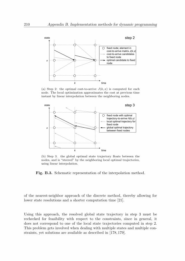
210 Appendix B. Implementation methods for dynamic programming
state
time k
x
step 2
optimization candi-dates for given node optimal solution for given node
fixed node; element in cost-to-arrive matrix J(k,x) cost-to-arrive candidates to fixed node optimal candidate to fixed node
(a) Step 2: the optimal cost-to-arrive J(k, x) is computed for eachnode. The local optimization approximates the cost at previous timeinstant by linear interpolation between the neighboring nodes.
state
time k
x
step 3
fixed node with optimal trajectory-to-arrive H(k,x) local optimal trajectory for fixed node global optimal trajectory between fixed nodes
(b) Step 3. the global optimal state trajectory floats between thenodes, and is “steered” by the neighboring local optimal trajectories,using linear interpolation.
Fig. B.3. Schematic representation of the interpolation method.
of the nearest-neighbor approach of the discrete method, thereby allowing forlower state resolutions and a shorter computation time [21].
Using this approach, the resolved global state trajectory in step 3 must berechecked for feasibility with respect to the constraints, since in general, itdoes not correspond to one of the local state trajectories computed in step 2.This problem gets involved when dealing with multiple states and multiple con-straints, yet solutions are available as described in [178,179].

B.4 Implementation 211
B.4.3 Hamiltonian method
The new Hamiltonian method introduced in this chapter extends the discretemethod by allowing each node to float within a local state space around a fixedpoint, instead of restricting the node to be on the fixed point, as schematicallyshown in Fig. B.4. The state trajectories are therefore not restricted to the dis-crete framework, yet for each local state space and each time instant, the optimalcost-to-arrive and associated trajectory-to-arrive are still stored in the optimiza-tion matrices. This approach allows for a straightforward implementation as inthe discrete method without interpolations, yet avoids the optimization errorcaused by state round offs.
The (continuous) state trajectory can be decomposed into the quantized globalstate bxe and its residual, the local state x − bxe. Using this separation, thetrajectory-to-arrive obtained in step 2 can be stored in two matrices, i.e., theglobal matrix H(k + 1, x(k + 1)) = bx(k)e, similar to the other methods, andan additional local matrix R(k + 1, x(k + 1)) = x(k) − bx(k)e that enables toreconstruct the original state trajectory. The dynamics of the local dynamicscan be described by
r(k, bx(k)e) =R(k + 1, x(k + 1))−R(k, x(k))
∆t. (B.22)
The local optimization around each node is different from previous methods,since the optimization candidates are allowed to have a different local state, asshown in Fig. B.4(a). Therefore, the local state dynamics are augmented tothe cost function given by (B.14) using an adjoined multiplier function λ(k),which assigns an equivalent cost of the local state evolution, resulting in theHamiltonian function. The local optimization problem then becomes
J(k + 1, bx(k + 1)e) = minu(k)∈U(k,x(k))
J(k, x(k)) + g(k, x(k), u(k))∆t
+λ(k)r(k, x(k))∆t . (B.23)
subject to the dynamics (B.9) and the state constraints (B.11). After computingthe optimal cost-to-arrive matrix J(k, x), the optimal trajectory-to-arrive matri-ces H(k, x) and R(k, x), the globally optimal trajectory can be resolved similarto the discrete method as shown in Fig. B.4(b), where the globally optimal tra-jectory follows the locally optimal trajectories.
The effectiveness of this method lies in the estimation of the optimal multiplierfunction λ(k), which is in general unknown. The optimal multiplier functioncan be interpreted as the “price” of state evolution, which can be approximated

212 Appendix B. Implementation methods for dynamic programming
state
time
local state space
optimization candi-dates for given node optimal solution for given node
R(k,x)
k
x
step 2
floating node; element in cost-to-arrive matrix J(k,x) cost-to-arrive candidates for local state space optimal candidate for local state space
(a) Step 2: the optimal cost-to-arrive J(k, x) is computed for a lo-cal state space around each node. The local optimization problemaugments the dynamics of the local state (i.e., distance between thecontinuous state and neighboring node) with a multiplier function toconsider the equivalent cost of state evolution.
R(k,x)
state
time
local state space
k
x
step 3
floating node with optimal trajectory-to-arrive H(k,x) local optimal trajectory for floating node global optimal trajectory
(b) Step 3. the global optimal state trajectory follows the local op-timal trajectories stored in H(k, x) and jumps from floating node tofloating node.
Fig. B.4. Schematic representation of the Hamiltonian method.
as a function of time and state if sufficient system knowledge is available. Theimpact of an inaccurate multiplier function on the found solution is discussed inthe sequel, assuming a constant estimation given by
λ(k) ≈ λ. (B.24)
From (B.23), it follows that for λ = 0, the last term of the cost function vanishesand the cost function reduces to its original (B.14). So, the solution is obtainedcompletely numerically, but the difference with the discrete method is that the

B.4 Implementation 213
state trajectory remains continuous, and is not manipulated by beneficial round-ing offs. For an incorrect multiplier function, the optimization accuracy can onlybe high if the quantized state resolution is high, such that the bounds on the localstate dynamics r(k, x(k), u(k)) diminish, and the last term of the cost functionwould become negligible even with the optimal multiplier function. For a rea-sonable estimate of the multiplier function, on the other hand, the quantizationresolution can be substantially reduced, thereby relying on a close-to-optimalsolution for the local optimization problem. If the optimal multiplier functionis exactly known, the resolution can be decreased to only one node per timeinstant, so the local state becomes the global state and the optimal solution isfound completely analytically. These observations give an interpretation of thisimplementation method: the global state trajectories are optimized numerically,whereas the local state trajectories are optimized analytically, where the quanti-zation resolution for the state determines the impact of each optimization. For awell estimated multiplier function, a high optimization accuracy can be obtainedwith a relatively low state resolution, resulting in a relatively short computationtime.
B.4.4 Computational efficiency
The computational efficiency of the dynamic programming algorithm can beimproved by reducing the memory usage and the total computation tim. Thememory usage can be substantially improved by using a relatively low numericalprecision, since the optimization accuracy is limited by the errors introducedby the quantization and mathematical modeling. In practice, a word lengthof only 32 bit is sufficiently accurate for the accumulated variables, and 16 bitfor the other variables, which are both much shorter than the double-precisionword length that uses 80 bit of the internal memory, e.g., standardly used inMatlab. The computation time can be substantially improved by implementingcustom interpolation functions, instead of the standard functions, e.g., interp1,interp2, and interp3 in Matlab, which are not optimized for computationalspeed due to rigorous error checks [21]. An alternative is to use parametricfunctions instead of multi-dimensional look-up tables to describe the dynamicsand incremental cost. The computation time can be improved significantly bycomputing the dynamics f(k, x(k), u(k)) and incremental cost g(k, x(k), u(k))a priori on each node (i.e., in step 1), for only the time instants with uniqueexternal states. For example, for the optimal control of a hybrid powertrain,only 60% of the time samples of six representative driving cycles2 contain an
2The selected driving cycles are the New European Driving Cycle (NEDC), the “low”,“medium”, and “high” parts of the Worldwide harmonized Light vehicles Test Procedure(WLTP), the Federal Test Procedure ’75 (FTP75), the sportive Eindhoven driving cycle(EHV), the Japan Cycle 08 (JC08), and the “urban” part of the Common Artemis DrivingCycle (CADC), as shown in Chapter 3.

214 Appendix B. Implementation methods for dynamic programming
Table B.1. Number of unique samples for six representative drivingcycles.
driving cycle time samples [-] unique samples [-] reduction
NEDC 1180 248 −79.0 %WLTP 1477 1146 −22.4 %FTP75 1877 938 −50.0 %EHV 879 698 −20.6 %JC08 1204 790 −34.4 %CADC 993 656 −33.9 %
total 7610 4476 −41.2 %
unique combination of the vehicle velocity and vehicle acceleration, as shown inTable B.1.
B.5 Case study: mechanical hybrid powertrain
As a case study, the design of an optimal energy controller for a mechanicalhybrid powertrain is considered, which uses only mechanical components forenergy storage and power transmission. This section summarizes the modelingand problem formulation, which are extensively described in Chapter 3.
B.5.1 System description
The topology of the mechanical hybrid powertrain is schematically depicted inFig. B.5. The main components are a 4-cylinder 1.5-l gasoline internal combus-tion engine, a vacuum-placed 150-kJ flywheel system, three clutches, a mass-produced pushbelt CVT, and a compact vehicle including 2 passengers with acurb weight of 1120 kg. The longitudinal (motion) dynamics are described forthe most relevant (largest) inertias, i.e., that of the flywheel and the vehicle.The transmission clutch (Ct) is used to transmit high powers while slipping,e.g., to accelerate the vehicle from standstill, which may take several time steps.The engine clutch (Ce) and the flywheel system clutch (Cf) are not designed totransmit high powers while slipping, yet to select driving modes by mechanical(dis-)engagement of powertrain parts, within one discrete time step of ∆t = 1 s.The powertrain can be operated in three relevant driving modes φ, which are
• Flywheel driving : the flywheel propels or brakes the vehicle while the en-gine is shut-off (φ = 1).
• Hybrid driving : the engine propels the vehicle while energizing the flywheel(φ = 2).

B.5 Case study: mechanical hybrid powertrain 215
Ce
Cf
Ct
engine
CVT
rotor
flywheel system
wheels
gears
clutches
Fig. B.5. Schematic overview of the mechanical hybrid powertraintopology that consists of an internal combustion engine, flywheel system,clutches, gears, and CVT.
• Engine driving : the engine propels the vehicle while the flywheel is coasting(φ = 3).
The flywheel system adds the following fuel saving functionalities: i) brake en-ergy recuperation for later use; ii) elimination of inefficient part-load operationof the engine, e.g., by flywheel driving, or by hybrid driving at a fuel-efficient op-eration point of the engine; iii) engine shutoff during vehicle standstill, where theflywheel is used to crank the engine. Physical constraints apply to the torques,the rotational speeds, and the speed ratio of the CVT, whereas comfort-relatedconstraints apply to driving mode switches that are expected to be uncomfort-able (i.e., slow, or with a torque interruption), which depend on the drivingconditions.
B.5.2 Problem formulation
The dynamic model can be described as in (B.9), where the state vector x con-tains the kinetic energy in the rotor of the flywheel system Er and the previousdriving mode φpre. The control variable vector u controls the driving mode φand the relative power split σ, which describes the power distribution betweenthe engine and flywheel system in the hybrid driving mode, i.e., σ = 0 impliesno flywheel energizing nor flywheel propulsion and σ = 1 implies maximal fly-wheel energizing. The external states are the prescribed vehicle velocity andacceleration, which are implied in the time vector (k). The objective is to min-imize the overall fuel consumption Ef (expressed in energy), over a pre-defineddriving cycle of length kn, subject to the system’s kinematics and dynamics, thephysical and comfort-related constraints, and no final state constraint, due to

216 Appendix B. Implementation methods for dynamic programming
its irrelevance for a short-term energy carrier such as the flywheel system. Thisoptimal control problem is characterized by
• switched dynamics due to discrete driving modes,
• active state constraints, such as on the energy state of the flywheel system
• non-convex control variable constraints to avoid uncomfortable drivingmode switches.
This class of optimization problems is relatively difficult to solve analytically,which makes dynamic programming very suitable to find the globally optimalsolution numerically. For the numerical optimization, the flywheel energy state(Er) is quantized with an equidistant distribution of n1 values, and the relativepower split (σ) is quantized with an equidistant distribution of 20 values. The(previous) driving mode (φ and φpre) are discrete variables (with 3 possiblevalues), hence need no quantization. The continuous state is implemented usingthe new Hamiltonian method, as well as the conventional discrete method toillustrate the differences in optimization performance. The interpolation methodis not implemented, as it is less suitable for this optimal control problem due tothe discrete control variable (driving mode) and the active state constraints.
B.6 Results
A set of simulations is performed to answer two research questions: i) Whatis a good estimate for the multiplier λ of the Hamiltonian method? ii) Whatis the optimization accuracy and computation time of the two implementationmethods as a function of the quantization resolution?
B.6.1 Multiplier estimation
The considered optimal control problem has one continuous state, i.e., the fly-wheel energy Er, for which the multiplier function is estimated by a constantvalue. Fig. B.6 shows the relative impact of the multiplier estimate λ ∈ [−7, 0]on the optimized fuel consumption (Ef) for six representative driving cycles. Forthese simulations, a relatively low resolution is selected for the energy state, ofonly n1 = 8 values, to amplify the effect of the multiplier estimate on the overallfuel consumption. Recall that a good estimate is desired to reduce the computa-tion time, since then a low resolution gives a sufficiently accurate result. It canbe seen that similar curves are obtained for each driving cycle, showing a globaloptimum around −3.0. As expected, the (absolute) optimal value resemblesvery well the average fuel-to-flywheel-energy conversion factor of −3.2, whichis usually used as a first estimate for the equivalent consumption minimization

B.6 Results 217
Ef(
λ)/
Ef(
λ=
0)[-]
λ [-]
−7 −6 −5 −4 −3 −2 −1 0
0.85
0.9
0.95
1
1.05
1.1
averageNEDCWLTPFTP75EHVJC08CADC
Fig. B.6. The relative impact of the constant multiplier estimate (λ) onthe optimized fuel consumption for six representative driving cycles.
strategy that is based on analytical optimization [118]. For this course grid reso-lution, up to 14% of the fuel consumption is reduced by optimizing the constantmultiplier. However, the sensitivity to the multiplier reduces with higher gridresolutions, together with the overal optimization error.
B.6.2 Optimization performance
The optimization performance of the Hamiltonian method and the discretemethod are evaluated for the NEDC for n1 ∈ [4, 1024] and λ = −3. As theperformance criteria, the accuracy of the optimized fuel consumption (Ef) andthe computation time (tcomp) are selected. The state resolution is an importantparameter that determines the trade-off between the optimization accuracy andthe computation time. Fig. B.7 shows the impact of the state resolution onthe relative optimized error and the relative computation time, with respect toa reference obtained with a relatively high state resolution of n∗1 = 2048 (i.e.,energy resolution of 150/2048 ≈ 73 J), using the discrete method, which givesalmost an identical result as the Hamiltonian method with this resolution.
For both implementation methods, a low resolution gives a short computationtime, yet at the cost of an inaccurate solution, and vice versa, as expected. Ascan be seen, the Hamiltonian method is superior to the discrete method forall investigated state resolutions. For a given resolution, the computation timeof the Hamiltonian method is slightly higher than the discrete method (2.5%on average), as it is mainly determined by the computation of the dynamics(f(k, x, u)) and the incremental cost (g(k, x, u)) for each node (k, x) and controlvariable (u), which remains the same for both implementation methods. The op-timization error, on the other hand, is substantially lower (factor 8.4 on average).
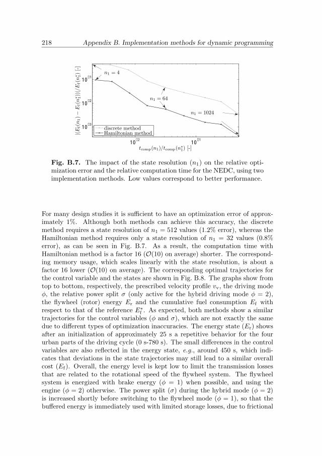
218 Appendix B. Implementation methods for dynamic programming
tcomp(n1)/tcomp(n∗1) [-]
|(Ef(
n1)−
Ef(n
∗ 1))|/E
f(n
∗ 1)
[-]
10−2
10−1
10−3
10−2
10−1
discrete methodHamiltonian method
n1 = 4
n1 = 64
n1 = 1024
Fig. B.7. The impact of the state resolution (n1) on the relative opti-mization error and the relative computation time for the NEDC, using twoimplementation methods. Low values correspond to better performance.
For many design studies it is sufficient to have an optimization error of approx-imately 1%. Although both methods can achieve this accuracy, the discretemethod requires a state resolution of n1 = 512 values (1.2% error), whereas theHamiltonian method requires only a state resolution of n1 = 32 values (0.8%error), as can be seen in Fig. B.7. As a result, the computation time withHamiltonian method is a factor 16 (O(10) on average) shorter. The correspond-ing memory usage, which scales linearly with the state resolution, is about afactor 16 lower (O(10) on average). The corresponding optimal trajectories forthe control variable and the states are shown in Fig. B.8. The graphs show fromtop to bottom, respectively, the prescribed velocity profile vv, the driving modeφ, the relative power split σ (only active for the hybrid driving mode φ = 2),the flywheel (rotor) energy Er and the cumulative fuel consumption Ef withrespect to that of the reference E∗f . As expected, both methods show a similartrajectories for the control variables (φ and σ), which are not exactly the samedue to different types of optimization inaccuracies. The energy state (Er) showsafter an initialization of approximately 25 s a repetitive behavior for the foururban parts of the driving cycle (0 s-780 s). The small differences in the controlvariables are also reflected in the energy state, e.g., around 450 s, which indi-cates that deviations in the state trajectories may still lead to a similar overallcost (Ef). Overall, the energy level is kept low to limit the transmission lossesthat are related to the rotational speed of the flywheel system. The flywheelsystem is energized with brake energy (φ = 1) when possible, and using theengine (φ = 2) otherwise. The power split (σ) during the hybrid mode (φ = 2)is increased shortly before switching to the flywheel mode (φ = 1), so that thebuffered energy is immediately used with limited storage losses, due to frictional

B.7 Conclusions 219
power dissipation in the flywheel system. On the highway part (910 s-1130 s),the engine mode (φ = 3) is selected as the engine can operated efficiently atrelatively high loads. A clear difference in the energy state (Er) is observedbetween the two methods, where the flywheel system appears to have no draglosses at low energy levels with the discrete method. This illustrates the maindrawback of the discrete method, which takes advantage of the round-off errorof the energy state, thereby virtually creating “free” energy when approximat-ing the system dynamics with (B.19). As a result for the discrete method, thecumulative fuel consumption (Ef) becomes increasingly lower than that of thereference solution (E∗f ), whereas for the Hamiltonian method, the cumulativefuel consumption becomes increasingly higher due to the sub-optimality.
B.7 Conclusions
Dynamic programming is an effective numerical optimization method to solverelatively complex optimal control problems, such as those characterized byswitched dynamics, active state constraints, and non-convex control constraints.The implementation of continuous states in the discrete framework, however,may lead to significant optimization inaccuracies. This chapter has presented anew implementation method that extends the conventional discrete method bystoring the quantization residual of the state, and augmenting the local dynam-ics of this residual to the local cost function, resulting in a Hamiltonian function.This Hamiltonian method can be interpreted as a mix between the analyticaland numerical methods, where the impact of each method is determined by theresolution of the quantized state. As a case study, to illustrate the effectivenessof this method, the optimal energy controller of a mechanical hybrid powertrainis computed. Results show that the optimization accuracy of the Hamiltonianmethod is superior to that of the discrete method. For a given desired opti-mization accuracy (≈ 1%), the computation time is substantially reduced, onaverage by a factor 8.2, whereas the corresponding memory usage is reduced by asimilar factor. This substantial reduction in computational time enables the useof dynamic programming for extensive parameter variation studies, such as theoptimization of the hybrid powertrain topology [24, 180] as described in Chap-ter 2, and for dynamic systems described by more states, such as the combinedenergy and thermodynamics in a hybrid powertrain as described in Chapter 4,or the combined energy and torque dynamics in a hybrid powertrain [149]. Italso allows for efficient computing of the explicit model predictive controller asdescribed in Chapter 5.

220 Appendix B. Implementation methods for dynamic programming
v v[m
/s]
0
10
20
30
φ[-]
1
2
3
σ[-]
0
0.5
1
Er
[kJ]
0
50
100
150
Ef−
E∗ f
[kJ]
time [s]
0 200 400 600 800 1000
−200
0
200
discrete methodHamiltonian method
Fig. B.8. The optimal solution for the discrete method and the Hamilto-nian method with a similar relative optimization error of approximately1%, using different quantization resolutions for the continuous energystate (Er).

Bibliography
[1] International Energy Agency, “Energy outlook 2010 - executive summary,” 2010.
[2] International Handling Services Automotive, “IHS automotives light vehicle pow-ertrain forecasts - global powertrain summary,” February 2013.
[3] H. Naunheimer, B. Bertsche, J. Ryborz, and W. Novak, Automotive Transmis-sions. Springer-Verlag, Berlin, Germany, 2nd ed., 2011.
[4] B. Vroemen, P. Debal, L. Romers, and M. Maessen, “Mechybrid; a low-costmechanical hybrid,” in Proc. of the 6th Int. Conf. on Continuously Variable andHybrid Transmissions, Maastricht, Netherlands, pp. 194–199, 2010.
[5] R. van Druten, Transmission design of the zero inertia powertrain. PhD thesis,Technische Universiteit Eindhoven, Netherlands, 2001.
[6] D. Meekhun, V. Boitier, and J. Dilhac, “Study of the ambient temperature effecton the characteristics and the lifetime of nickel-metal hydride secondary battery,”in Proc. of the Electrical Power & Energy Conference (EPEC), Canada, pp. 1–4,2009.
[7] F. Thoolen, Development of an advanced high speed flywheel energy storage sys-tem. PhD thesis, Technische Universiteit Eindhoven, Netherlands, 1993.
[8] K. van Berkel, L. Romers, B. Vroemen, T. Hofman, and M. Steinbuch, “Per-formance simulations of a low-cost hybrid powertrain with large fuel savings,”International Journal of Powertrains, vol. 1, no. 4, pp. 377–395, 2012.
[9] S. van der Meulen, High-performance Control of Continuously Variable Trans-missions. PhD thesis, Technische Universiteit Eindhoven, Netherlands, 2010.
[10] D. Kok, Design optimization of a flywheel hybrid vehicle. PhD thesis, TechnischeUniversiteit Eindhoven, Netherlands, 1999.
[11] A. Serrarens, Coordinated control of the zero inertia powertrain. PhD thesis,Technische Universiteit Eindhoven, Netherlands, 2001.
[12] J. Kessels, Energy Management for Automotive Power Nets. PhD thesis, Tech-nische Universiteit Eindhoven, Netherlands, 2007.
[13] B. Vroemen, Component Control for The Zero Inertia Powertrain. PhD thesis,Technische Universiteit Eindhoven, Netherlands, Eindhoven, 2001.

222 Bibliography
[14] D. Kirk, Optimal Control Theory: an Introduction. Prentice-Hall Inc., NewJersey, 1970.
[15] L. S. Pontryagin, V. G. Boltyanskii, R. V. Gamkrelidze, and E. F. Mishchenko,The Mathematical Theory of Optimal Processes. Interscience Publishers, NewYork, 1962.
[16] H. P. Geering, Optimal Control with Engineering Applications. Springer-VerlagBerlin Heidelberg, 2007.
[17] R. Bellman, Dynamic Programming. Princeton University Press, 1957.
[18] D. P. Bertsekas, Dynamic Programming and Optimal Control, Volume 1. AthenaScientific, Belmont, Massachusetts, U.S.A., 3rd ed., 2005.
[19] D. P. Bertsekas, Dynamic Programming and Optimal Control, Volume 2. AthenaScientific, Belmont, Massachusetts, U.S.A., 3rd ed., 2005.
[20] T. van Keulen, Fuel Optimal Control of Hybrid Vehicles. PhD thesis, TechnischeUniversiteit Eindhoven, Netherlands, 2011.
[21] L. Guzzella and S. Sciarreta, Vehicle propulsion systems: introduction to model-ing and optimization. Springer-Verlag, Berlin, Germany, 2nd ed., 2007.
[22] U. Christen and R. Busch, “The art of control engineering: science meets in-dustrial reality,” in Proc. of the IFAC ECOSM 12, Rueil-Malmaison, France,2012.
[23] T. Hofman, Framework for Combined Control and Design Optimization of Hy-brid Vehicle Propulsion Systems. PhD thesis, Technische Universiteit Eindhoven,Netherlands, 2007.
[24] S. Ebbesen, Optimal sizing and control of hybrid electric vehicles. PhD thesis,Swiss Federal Institute of Technology, Zurich, 2012.
[25] G. Vogelaar, “VT2+: further improving the fuel economy of the VT2 trans-mission,” in Proc. of the 6th Int. Conf. on Continuously Variable and HybridTransmissions, Maastricht, Netherlands, pp. 105–109, 2010.
[26] L. Guzzella and C. Onder, Introduction to Modeling and Control of InternalCombustion Engine Systems. Springer-Verlag, 2nd ed. ed., 2010.
[27] J. Dolcini, C. de Wit, and H.Bechart, Dry Clutch Control for Automotive Appli-cations. Springer-Verlag, London, United Kingdom, 2010.
[28] J. Hilton, “Flywheel hybrid as an alternative to electric vehicles,” Automobil-technische Zeitschrift Worldwide, vol. 114, pp. 26–30, 2012.
[29] K. van Berkel, L. Romers, T. Hofman, B. Vroemen, and M. Steinbuch, “Designof a low-cost hybrid powertrain with large fuel savings,” in Proc. of the 25th Int.Electric Vehicle Symposium, Shenzhen, China, 2010.
[30] C. Brockbank, “Development of full-toroidal traction drive in flywheel basedmechanical hybrids,” in Proc. of the 6th Int. Conf. on Continuously Variableand Hybrid Transmissions, Maastricht, Netherlands, pp. 163–169, 2010.
[31] H. Kuipers, “Geschiedenis van de autobus,” De Alkenreeks; beeld-encyclopedie,vol. 146, p. 64 pages, 1967.

Bibliography 223
[32] C. Brockbank and C. Greenwood, “Formula 1 mechanical hybrid applied to main-stream automotive,” in VDI Getriebe in Fahrzeuge Conference, 2008.
[33] M. van Drogen and M. van der Laan, “Determination of variator robustnessunder macro slip conditions for a push belt CVT,” SAE Transactions, vol. 114,no. 6, pp. 232–246, 2004.
[34] T. Doi, “New compact, lightweight, low friction CVT with wide ratio coverage,”in Proc. of the 6th Int. Conf. on Continuously Variable and Hybrid Transmis-sions, Maastricht, Netherlands, 2010.
[35] K. van Berkel, S. Rullens, T. Hofman, B. Vroemen, and M. Steinbuch, “Anal-ysis of optimal mechanical-hybrid powertrain topologies,” in Proc. of the IFACECOSM 12, Rueil-Malmaison, France, pp. 61–68, 2012.
[36] S. Delprat, T. Guerra, and J. Rimaux, “Optimal control of a parallel powertrain:From global optimization to realtime control strategy,” in Proc. of the IEEE 55thVehicular Technology Conference, Birmingham, vol. 4, pp. 2082–2088, 2002.
[37] J. Kessels, M. Koot, P. van den Bosch, and D. Kok, “Online energy managementfor hybrid electric vehicles,” IEEE Transactions on Vehicular Technology, vol. 57,no. 6, pp. 3428–3440, 2008.
[38] T. van Keulen, D. van Mullem, B. de Jager, J. T. Kessels, and M. Steinbuch,“Design, implementation, and experimental validation of optimal power splitcontrol for hybrid electric trucks,” Control Engineering Practice, vol. 20, pp. 547–558, May 2012.
[39] T. Hofman, S. Ebbesen, and L. Guzzella, “Topology optimization for hybridelectric vehicles with automated transmissions,” IEEE Transactions on VehicularTechnology, vol. 61, no. 6, pp. 2442–2451, 2012.
[40] I. Kolmanovsky and A. Stefanopoulou, “Optimal control techniques for assessingfeasibility and defining subsystem level requirements: an automotive case study,”IEEE Transactions on Control Systems Technology, vol. 9, no. 3, pp. 524–534,2001.
[41] P. Dietrich, H. Horler, and M. Eberle, “The ETH-hybrid car - a concept to mini-mize consumption and reduce emissions,” in Proc. of the 26th ISATA Conference,Aachen, Germany, 1999.
[42] Y. Huang, “A hybrid power driving system with an energy storage flywheel forvehicles,” in Proc. of the SAE Comm. Veh. Eng. Congress, Rosemont, Illinois,U.S.A., pp. 1–10, 2007.
[43] P. Acarnley, B. Mecrow, J. Burdess, J. Fawcett, J. Kelly, and P. Dickinson, “De-sign principles for a flywheel energy store for road vehicles,” IEEE Transactionson Industry Applications, vol. 32, no. 6, pp. 1402–1408, 1996.
[44] S. Wright, Control of IVT-Based Vehicles by Intelligent Selection Between Alter-native Solutions. PhD thesis, University of Lancaster, U.K., 2006.
[45] S. Shen, A. Serrarens, M. Steinbuch, and F. Veldpaus, “Coordinated control ofa mechanical hybrid driveline with a continuously variable transmission,” JSAEReview, vol. 22, no. 4, pp. 453–461, 2001.

224 Bibliography
[46] R. van Druten, M. Pesgens, B. Vroemen, and A. Serrarens, “Performance analysisof the impuls shift transmission,” VDI Berichte, no. 1852, pp. 237–253, 2004.
[47] E. Galvagno, M. Velardocchia, and A. Vigliani, “A model for a flywheel automaticassisted manual transmission,” Mechanism and Machine Theory, vol. 44, no. 6,pp. 1294 – 1305, 2009.
[48] L. Lawson, “Is there a flywheel in your future?,” SAE Technical Paper 730621,pp. 248–255, 1973.
[49] A. A. Frank and N. H. Beachley, “Evaluation of the flywheel drive concept forpassenger vehicles,” SAE Technical Paper 790049, pp. 1–12, 1979.
[50] C. M. Jefferson and M. Ackerman, “A flywheel variator energy storage system,”Energy Conversion and Management, vol. 37, no. 10, pp. 1481–1491, 1996.
[51] A. Barr and A. Veshagh, “Fuel economy and performance comparison of alterna-tive mechanical hybrid powertrain configurations,” in World Congress, Detroit,Michigan, U.S.A., no. 2008-01-0083, 2008.
[52] D. Moro, N. Cavina, I. Trivi, and V. Ravaglioli, “Guidelines for integration ofkinetic energy recovery system (kers) based on mechanical flywheel in an auto-motive vehicle,” SAE Technical Paper 2010-01-1448, 2010.
[53] K. Pullen and C. Ellis, “Kinetic energy storage for vehicles,” in Hybrid VehicleConference, Conventry, United Kingdom, pp. 91–108, 2006.
[54] U. Diego-Ayala, P. Martinez-Gonzalez, N. McGlashan, and K. Pullen, “The me-chanical hybrid vehicle: an investigation of a flywheel-based vehicular regener-ative energy capture system,” Proc. IMechE, J. of Automobile Eng., vol. 222,no. 11, pp. 2087–2101, 2008.
[55] H.-K. Su and T. Liu, “Design and analysis of hybrid power systems with variableinertia flywheel,” World Electric Vehicle Journal, vol. 4, pp. 452–459, 2010.
[56] N. A. Schilke, A. O. Dehart, L. O. Hewko, C. C. Matthews, D. J. Pozniak,and S. M. Rohde, “The design of an engine-flywheel hybrid drive system for apassenger car,” SAE Technical Paper 841306, pp. 255–275, 1984.
[57] C. J. Greenwood, “Driveline for regenerative braking,” May 1985.
[58] C. J. Greenwood, “Integration of a commercial vehicle regenerative braking driv-eline,” IMechE, vol. 191, pp. 127–133, 1986.
[59] R. van der Graaf, “An IC engine-flywheel hybrid drive for road vehicles,” inEAEC-Congress, Strasbourg, France, no. 87031, 1987.
[60] E. Spijker, “An electronically controlled CVT for a flywheel-hybrid vehicle trans-mission,” in Proc. of thee ISATA Mechatronics Conference, Aachen, Germany,pp. 281–288, 1993.
[61] D. Kok, R. v. d. Graaf, and R. Kriens, “Validation of a high efficiency flywheelhybrid driveline concept,” in FISITA World Automotive Congress, Prague, CzechRepublic, 1996.
[62] R. Stone and C. Brockbank, “Developments leading to series production ap-plications of torotrak’s full-toroidal traction drive technology,” in Proc. of the6th Int. Conf. on Continuously Variable and Hybrid Transmissions, Maastricht,Netherlands, pp. 170–177, 2010.

Bibliography 225
[63] K. Wipke, M. Cuddy, and S. Burch, “Advisor 2.1: A user-friendly advanced pow-ertrain simulation using a combined backward/forward approach,” IEEE Trans-actions On Vehicular Technology, vol. 48, no. 6, pp. 1751–1761, 1999.
[64] K. van Berkel, T. Hofman, B. Vroemen, and M. Steinbuch, “Optimal regenerativebraking with a push-belt CVT: an experimental study,” in Proc. of the 10th Int.Symp. on Advanced Vehicle Control, Loughborough, U.K., pp. 67–72, 2010.
[65] S. Di Cairano, D. Yanakiev, A. Bemporad, I. Kolmanovsky, and D. Hrovat,“Model predictive idle speed control: Design, analysis, and experimental evalua-tion,” IEEE Transactions on Control Systems Technology, vol. 20, no. 1, pp. 84–97, 2012.
[66] K. van Berkel, T. Hofman, B. Vroemen, and M. Steinbuch, “Optimal control ofa mechanical-hybrid powertrain,” IEEE Transactions on Vehicular Technology,vol. 61, no. 2, pp. 485–497, 2012.
[67] K. van Berkel, M. Maessen, T. Hofman, B. Vroemen, and M. Steinbuch, “Semi-empirical power dissipation modeling of mechanical hybrid powertrain compo-nents,” under review for journal publication, 2013.
[68] L. van Dongen, “Efficiency characteristics of manual and automatic passengercar transaxles,” SAE Technical Paper, 1982.
[69] M. Ehsani, Y. Gao, and A. Emadi, Modern electric, hybrid electric, and fuel cellvehicles : fundamentals, theory, and design. London: CRC Press, 2010.
[70] A. Kade, A. J. Walenty, and K. G. Leppek, “Regenerative and friction brakeblend control,” 1996.
[71] K. van Berkel, B. de Jager, T. Hofman, B. Vroemen, and M. Steinbuch, “Imple-mentation of dynamic programming for optimal control problems with continuousstates,” under review for journal publication, 2013.
[72] A. Anderson and R. Knapp, “Hot spotting in automotive friction systems,” Wear,vol. 135, no. 2, pp. 319–337, 1990.
[73] A. Sciarretta and L. Guzzella, “Control of hybrid electric vehicles,” IEEE ControlSystems, vol. 27, no. 2, pp. 60–70, 2007.
[74] F. Salmasi, “Control strategies for hybrid electric vehicles: Evolution, classifica-tion, comparison, and future trends,” IEEE Transactions On Vehicular Technol-ogy, vol. 56, no. 5, pp. 2393–2404, 2007.
[75] C. Wittmer, L. Guzella, and P. Dietrich, “Optimized control strategies for a hy-brid car with a heavy flywheel,” Automatisierungstechnik, vol. 44, no. 7, pp. 331–337, 1996.
[76] M. Ehsani, Y. Gao, and A. Emad, Modern electric, hybrid electric and fuel cellvehicles: fundamentals, theory and design. CRC Press, Boca Raton, Florida,USA, 2nd ed., 2005.
[77] J. Hellgren and E. Jonasson, “Maximisation of brake energy regeneration ina hybrid electric parallel car,” Int. J. of Electric and Hybrid Vehicles, vol. 1,pp. 95–121, 2007.

226 Bibliography
[78] M. Dodd and I. Knight, “Technical assistance and economic analysis in the field oflegislation pertinent to the issue of automotive safety: provision for informationand services on the subject to brake assist systems,” tech. rep., TRL Limited,2007.
[79] United Nations Economic Commission for Europe, “Worldwide harmonized lightvehicles test procedure, class 3, version 5.3,” tech. rep., 2012.
[80] M. Andre, “The ARTEMIS European driving cycles for measuring car pollutantemissions,” Science of The Total Environment, vol. 334-335, pp. 73–84, 2004.
[81] C. D. Chan, T. Yang, D. Volz, F. Breitweiser, A. Jamzadeh, T. Frank, andOmitsu, “System design and control considerations of automotive continuouslyvariable transmissions,” SAE Technical Paper 840048, 1984.
[82] S. Liu and B. Paden, “A survey of today’s CVT controls,” in 36th IEEE Con-ference on Decision and Control, vol. 5, pp. 4738–4743, 1997.
[83] R. Pfiffner, Optimal operation of CVT-based powertrains. PhD thesis, SwissFederal Institute of Technology, Zurich, 2001.
[84] D. V. Ngo, Gear Shift Strategies for Automotive Transmissions. PhD thesis,Technische Universiteit Eindhoven, Netherlands, 2012.
[85] D. Bolis, J. Johnson, and R. Callen, “A study on the effect of oil and coolanttemperatures on diesel engine brake specific fuel consumption,” SAE TechnicalPaper 770313, 1977.
[86] G. E. Andrews, J. R. Harris, and A. Ounzain, “SI engine warm-up: Water andlubricating oil temperature influences,” SAE Technical Paper 892103, 1989.
[87] P. Shayler, S. Christian, and T. Ma, “A model for the investigation of tem-perature, heat flow and friction characteristics during engine warm-up,” SAETechnical Paper 931153, pp. 667–675, 1993.
[88] T. Morel and R. Keribar, “Warmup characteristics of a spark ignition engine asa function of speed and load,” SAE Technical Paper 900683, 1990.
[89] K. Kunze, S. Wolff, I. Lade, and J. Tonhauser, “A systematic analysis of co2-reduction by an optimized heat supply during vehicle warm-up,” SAE TechnicalPaper 2006-01-1450, vol. 01, 2006.
[90] C. Haupt, D. Bucherl, A. Engstle, H.-G. Herzog, and G. Wachtmeister, “Energymanagement in hybrid vehicles considering thermal interactions,” in Proc. of theVehicle Power and Propulsion Conference, Arlington, Texas, U.S.A., pp. 36–41,2007.
[91] T. Mueller, H. Hans, W. Krebs, S. Smith, and A. Koenigstein, “Thermal man-agement on small gasoline engines,” SAE International, no. 2011-01-0314, 2011.
[92] F. Will and A. Boretti, “A new method to warm up lubricating oil to improvethe fuel efficiency during cold start,” SAE International, no. 2011-01-0318, 2011.
[93] R. Cipollone, D. D. Battista, and A. Gualtieri, “Head and block split coolingin internal combustion engines,” in Proc. of the IFAC Workshop on Engine andPowertrain Control, Simulation and Modeling, pp. 469–476, 2012.

Bibliography 227
[94] E. Muller, A. Stefanopoulou, and L. Guzzella, “Optimal power control of hybridfuel cell systems for an accelerated system warm-up,” IEEE Transactions onControl Systems Technology, vol. 15, no. 2, pp. 290–305, 2007.
[95] J. Lescot, A. Sciarretta, Y. Chamaillard, and A. Charlet, “On the integrationof optimal energy management and thermal management of hybrid electric ve-hicles,” in Proc. of the Vehicle Power and Propulsion Conference, Lille, France,pp. 1–6, 2010.
[96] R. Dubouil, J. F. Hetet, and A. Maiboom, “Modelling of the warm-up of a sparkignition engine: Application to hybrid vehicles,” SAE International, no. 2011-01-1747, 2011.
[97] K. van Berkel, W. Klemm, T. Hofman, B. Vroemen, and M. Steinbuch, “Optimalenergy management for a mechanical-hybrid vehicle with cold start conditions,”in Proc. of the European Control Conference, Zurich, Switzerland, p. 6, 2013.
[98] J. A. Kaplan and J. B. Heywood, “Modeling the spark ignition engine warm-upprocess to predict component temperatures and hydrocarbon emissions,” in SAEInternational Congress and Exposition, Detroit, Michigan, U.S.A., no. 910302,1991.
[99] O. Arici, J. H. Johnson, and A. J. Kulkarni, “The vehicle engine cooling systemsimulation part 1 - model development,” in SAE World Congress and Exposition,Detroit, Michigan, U.S.A., no. 1999-01-0240, 1999.
[100] L. Jarrier, J. C. Champoussin, R. Yu, and D. Gentile, “Warm-up of a d.i. dieselengine: Experiment and modeling,” in SAE World Congress, Detroit, Michigan,2000.
[101] T. Markel, A. Brooker, T. Hendricks, V. Johnson, K. Kelly, B. Kramer,M. O’Keefe, S. Sprik, and K. Wipke, “Advisor: a systems analysis tool for ad-vanced vehicle modeling,” Journal of Power Sources, vol. 110, no. 2, pp. 255–266,2002.
[102] R. Eichhorn, M. Boot, and C. Luijten, “Waste energy driven air conditioningsystem (WEDACS),” SAE Int. J. of Engines, vol. 2, no. 2, pp. 477–492, 2009.2009-24-0063.
[103] K. van Berkel, S. Rullens, T. Hofman, B. Vroemen, and M. Steinbuch, “Topologyand flywheel size optimization of mechanical hybrid powertrains,” under reviewfor journal publication, 2013.
[104] S. Delprat, J. Lauber, T. Guerra, and J. Rimaux, “Control of a parallel hy-brid powertrain: optimal control,” IEEE Transactions on Vehicular Technology,vol. 53, no. 3, pp. 872–881, 2004.
[105] D. Ambuhl, O. Sundstrom, A. Sciarreta, and L. Guzzella, “Explicit optimal con-trol policy and its practical application for hybrid electric powertrains,” ControlEngineering Practice, vol. 18, pp. 1429 – 1439, 2010.
[106] F. Allgower, T. Badgwell, J. Qin, and J. Rawlings, Nonlinear predictive con-trol and moving horizon estrimation an introductory overview. Springer-Verlag,London, UK, in advances in control, highlights of ECC99 ed., 1999.
228 Bibliography
[107] B. Glaser and A. Strauss, The discovery of grounded theory: Strategies for qual-itative research. Transaction Publishers, 7th ed., 2012.
[108] P. Papalambros and D. Wilde, Principles of Optimal Design. Cambridge Uni-versity Press, 2 ed., 2000.
[109] N. Kim and A. Rousseau, “Sufficient conditions of optimal control based on Pon-tryagin’s minimum principle for use in hybrid electric vehicles,” Proc. IMechE,J. of Automobile Eng., vol. 226, no. 9, pp. 1160–1170, 2012.
[110] D. F. Opila, X. Wang, R. McGee, R. B. Gillespie, J. A. Cook, and J. W. Grizzle,“An energy management controller to optimally trade off fuel economy and driv-ability for hybrid vehicles,” IEEE Transactions on Control Systems Technology,vol. 20, no. 6, pp. 1490–1505, 2012.
[111] K. van Berkel, W. Klemm, T. Hofman, B. Vroemen, and M. Steinbuch, “Optimalcontrol of a mechanical hybrid powertrain with cold start conditions,” underreview for journal publication, 2013.
[112] N. Kim, S. Cha, and H. Peng, “Optimal control of hybrid electric vehicles basedon Pontryagin’s minimum principle,” IEEE Transactions on Control SystemsTechnology, vol. 19, no. 5, pp. 1279–1287, 2011.
[113] D. Ngo, T. Hofman, M. Steinbuch, and A. Serrarens, “Optimal control of thegearshift command for hybrid electric vehicles,” IEEE Transactions on VehicularTechnology, vol. 61, no. 8, pp. 3531–3543, 2012.
[114] M. Koot, J. T. B. A. Kessels, B. de Jager, W. P. M. H. Heemels, P. P. J. van denBosch, and M. Steinbuch, “Energy management strategies for vehicular electricpower systems,” IEEE Transactions on Vehicular Technology, vol. 54, no. 3,pp. 771–782, 2005.
[115] W. B. Powell, Approximate Dynamic Programming, Solving the curses of dimen-sionality. John Wiley and Sons, 2nd ed., 2011.
[116] P. van den Bosch and F. Lootsma, “Scheduling of power generation via large-scale nonlinear optimization,” Journal of Optimization Theory and Applications,vol. 55, no. 2, pp. 313–326, 1987.
[117] G. Paganelli, S. Delprat, T. Guerra, J. Rimaux, and J. Santin, “Equivalentconsumption minimization strategy for parallel hybrid powertrains,” in VehicularTechnology Conference, vol. 4, pp. 2076–2081, 2002.
[118] A. Sciarretta, M. Back, and L. Guzzella, “Optimal control of parallel hybridelectric vehicles,” IEEE Transactions on Control Systems Technology, vol. 12,no. 3, pp. 352–363, 2004.
[119] C. Musardo, G. Rizzoni, and B. Staccia, “A-ECMS: An adaptive algorithm forhybrid electric vehicle energy management,” in Proc. of the 44th IEEE Confer-ence on Decision and Control, and the European Control Conference, Seville,Spain, pp. 1816–1823, 2005.
[120] I. Kolmanovsky, I. Siverguina, and B. Lygoe, “Optimization of powertrain oper-ating policy for feasibility assessment and calibration: stochastic dynamic pro-gramming approach,” in Proc. of the American Control Conference, Anchorage,AK, United States, pp. 1425–1430, 2002.

Bibliography 229
[121] E. D. Tate, J. W. Grizzle, and H. Peng, “Shortest path stochastic control forhybrid electric vehicles,” International Journal of Robust and Nonlinear Control,vol. 18, no. 14, pp. 1409–1429, 2007.
[122] M. Back, M. S. F. Kirschaum, and V. Krebs, “Predictive control of drivetrains,”in 15th IFAC Trennial World Congress, Barcelona, Spain, 2002.
[123] H. Borhan, A. Vahidi, A. Phillips, M. Kuang, I. Kolmanovsky, and S. Di Cairano,“Mpc-based energy management of a power-split hybrid electric vehicle,” IEEETransactions on Control Systems Technology, vol. 20, no. 3, pp. 593–603, 2012.
[124] C.-C. Lin, H. Peng, J. W. Grizzle, and J.-M. Kang, “Power management strat-egy for a parallel hybrid electric truck,” IEEE Transactions on Control SystemsTechnology, vol. 11, no. 6, pp. 839–849, 2003.
[125] A. Bemporad, F. Borrelli, L. Glielmo, and F. Vasca, “Hybrid control of dry clutchengagement,” in Proc. European Control Conference, Porto, Portugal, 2001.
[126] Y. Zhu, Y. Chen, G. Tian, H. Wu, and Q. Chen, “A four-step method to designan energy management strategy for hybrid vehicles,” in Proc. of the AmericanControl Conf., Boston Massachusetts, U.S.A., 2004.
[127] A. Emadi, K. Rajashekara, S. Williamson, and S. Lukic, “Topological overview ofhybrid electric and fuel cell vehicular power system architectures and configura-tions,” IEEE Transactions on Vehicular Technology, vol. 54, no. 3, pp. 763–770,2005.
[128] J. Slicker and R. Loh, “Design of robust vehicle launch control systems,” IEEETransactions On Control System Technology, vol. 4(4), pp. 326–335, 1996.
[129] M. Pettersson and L. Nielsen, “Gear shifting by engine control,” IEEE Transac-tions on Control Systems Technology, vol. 8, no. 3, pp. 495–507, 2000.
[130] J. Fredriksson and B. Egardt, “Nonlinear control applied to gearshifting in au-tomated manual transmissions,” in Decision and Control, 2000. Proceedings ofthe 39th IEEE Conference on, vol. 1, pp. 444–449, 2000.
[131] F. Garofalo, L. Glielmo, L. Ianelli, and F. Vasca, “Smooth engagement of auto-motive dry clutch,” in Proc. of the 40th IEEE CDC, pp. 529–534, 2001.
[132] A. Serrarens, M. Dassen, and M. Steinbuch, “Simulation and control of an au-tomotive dry clutch,” in Proc. of the American Control Conference, Boston,Massachusetts, U.S.A., vol. 5, pp. 4078–4083, 2004.
[133] L. Glielmo, L. Iannelli, V. Vacca, and F. Vasca, “Gearshift control for automatedmanual transmissions,” IEEE/ASME Transactions on Mechatronics, vol. 11,no. 1, pp. 17–26, 2006.
[134] H. Tanaka and H. Wada, “Fuzzy control of clutch engagement for automatedmanual transmission,” Vehicle System Dynamics, vol. 24, no. 4-5, pp. 365–376,1995.
[135] K. Hayashi, Y. Shimizu, Y. Dote, A. Takayama, and A. Hirako, “Neuro fuzzytransmission control for automobile with variable loads,” IEEE Transactions onControl Systems Technology, vol. 3, no. 1, pp. 49–53, 1995.
[136] M. Kulkarni, T. Shim, and Y. Zhang, “Shift dynamics and control of dual-clutchtransmissions,” Mechanism and Machine Theory, vol. 42, pp. 168–182, Feb. 2007.

230 Bibliography
[137] A. C. van der Heijden, A. F. A. Serrarens, M. K. Camlibel, and H. Nijmeijer,“Hybrid optimal control of dry clutch engagement,” Int. J. of Control, vol. 80,pp. 1717–1728, 2007.
[138] K. van Berkel, T. Hofman, A. Serrarens, and M. Steinbuch, “Fast and smoothclutch engagement control for dual-clutch transmissions,” under review for jour-nal publication, 2013.
[139] G. Naus, H. R. Beenakkers, M., M. v. d. Molengraft, and M. Steinbuch, “Ro-bust control of a clutch system to prevent judder-induced driveline oscillations,”Vehicle System Dynamics, vol. 48, no. 11, pp. 1379–1394, 2010.
[140] B. Gao, H. Chen, K. Sanada, and Y. Hu, “Design of clutch-slip controller for au-tomatic transmission using backstepping,” IEEE Transactions on Mechatronics,vol. 16, no. 3, pp. 498–508, 2011.
[141] F. Vasca, L. Iannelli, A. Senatore, and G. Reale, “Torque transmissibility assess-ment for automotive dry-clutch engagement,” IEEE Transactions on Mechatron-ics, vol. 16, no. 3, pp. 564–573, 2011.
[142] J. Deur, J. Petric, J. Asgari, and D. Hrovat, “Modeling of wet clutch engagementincluding a thorough experimental validation,” SAE Technical Paper, vol. 1,no. 877, p. 18 pages, 2005.
[143] J. Deur, J. Petric, J. Asgari, and D. Hrovat, “Recent advances in control-orientedmodeling of automotive power train dynamics,” IEEE/ASME Transactions onMechatronics, vol. 11, no. 5, pp. 513–523, 2006.
[144] B. Gao, H. Chen, H. Zhao, and K. Sanada, “A reduced-order nonlinear clutchpressure observer for automatic transmission,” IEEE Transactions on ControlSystems Technology, vol. 18, no. 2, pp. 446–453, 2010.
[145] S. van der Meulen, B. de Jager, F. Veldpaus, and M. Steinbuch, “Combiningextremum seeking control and tracking control for high-performance CVT op-eration,” in Proc. of the 49th IEEE Conf. on Decision and Control, Atlanta,U.S.A., pp. 3668–3673, 2010.
[146] G. F. Franklin and A. Emami-Naeini, Feedback Control of Dynamic Systems.Prentice-Hall, 4th ed. ed., 2001.
[147] J. H. Lambert, “Observations variae in mathesin puram,” Acta Helvitica, physico-mathematico-anatomico-botanico-medica, vol. 3, pp. 128–168, 1758.
[148] T. Hofman, M. Steinbuch, R. van Druten, and A. Serrarens, “Design of CVT-based hybrid passenger cars,” IEEE Transactions on Vehicular Technology,vol. 58, no. 2, pp. 572–587, 2009.
[149] T. Nuesch, M. Wang, C. Voser, and L. Guzzella, “Optimal energy managementand sizing for hybrid electric vehicles considering transient emissions,” in Proc.of the IFAC ECOSM 12, Rueil-Malmaison, France, pp. 211–218, 2012.
[150] D. Gao, C. Mi, and A. Emadi, “Modeling and simulation of electric and hybridvehicles,” Proceedings of the IEEE, vol. 95, no. 4, pp. 729–745, 2007.
[151] G. Rizzoni, L. Guzzella, and B. Baumann, “Unified modeling of hybrid electricvehicle drivetrains,” IEEE/ASME Transactions on Mechatronics, vol. 4, no. 3,pp. 246–257, 1999.

Bibliography 231
[152] T. Hofman, M. Steinbuch, R. van Druten, and A. Serrarens, “Rule-based en-ergy management strategies for hybrid vehicles,” Int. J. of Electric and HybridVehicles, vol. 1, pp. 71–94, 2007.
[153] E. Pennestri, L. Mariti, P. P. Valentini, and V. H. Mucino, “Efficiency evaluationof gearboxes for parallel hybrid vehicles: theory and applications,” Mechanismand Machine Theory, vol. 49, pp. 157–176, 2012.
[154] J. D. Micklem, D. K. Longmore, and C. R. Burrows, “Belt torque loss in a steelv-belt continuously variable transmission,” Proc. IMechE, J. of Automobile Eng.,vol. 208, no. 2, pp. 91–97, 1994.
[155] C. Zhu, H. Liu, J. Tian, Q. Xiao, and X. Du, “Experimental investigation on theefficiency of the pulley-drive CVT,” Int. J. of Automotive Technology, vol. 11,no. 2, pp. 257–261, 2010.
[156] T. Ide, “Effect of belt loss and oil pump loss on the fuel economy of a vehiclewith a metal v-belt CVT,” in Proc. of the FISITA World Automotive Congress,Seoul Korea, 2000.
[157] R. Pfiffner, L. Guzzella, and C. H. Onder, “Fuel-optimal control of CVT power-trains,” IFAC Control Engineering Practice, vol. 11, no. 3, pp. 329 – 336, 2003.
[158] J. D. Micklem, D. K. Longmore, and C. R. Burrows, “The magnitude of thelosses in the steel pushing v-belt continuously variable transmission,” Proc. ofthe IMechE, Part D: Journal of Automobile Engineering, vol. 210, no. 1, pp. 57–62, 1996.
[159] S. Kuwabara, T. Fujii, and S. Kanehara, “Power transmitting mechanisms ofCVT using a metal v-belt and load distribution in the steel ring,” SAE TechnicalPaper 980824, 1998.
[160] S. Akehurst, N. D. Vaughan, D. A. Parker, and D. Simner, “Modelling of lossmechanisms in a pushing metal v-belt continuously variable transmission: Part2: Pulley deflection losses and total torque loss validation,” Proc. of the IMechE,Part D: Journal of Automobile Engineering, vol. 218, no. 11, pp. 1283–1293,2004.
[161] K. Narita and M. Priest, “Metal-metal friction characteristics and the transmis-sion efficiency of a metal v-belt-type continuously variable transmission,” Proc.IMechE, J. of Eng. Tribology, vol. 221, pp. 11–26, 2007.
[162] G. Carbone, L. D. Novellis, G. Commissaris, and M. Steinbuch, “An enhancedCMM model for the accurate prediction of steady-state performance of CVTchain drives,” ASME J. of Mechanical Design, vol. 132, no. 2, pp. 1–8, 2010.
[163] F. Van der Sluis, “A new pump for CVT applications.,” SAE Technical Paper01-3207, 2003.
[164] B. Pennings, M. van Drogen, A. Brandsma, E. van Ginkel, and M. Lemmens,“Van Doorne CVT fluid testa test method on belt-pulley level to select fluids forpush belt CVT application,” SAE Technical Paper 2003-01-3253, 2003.
[165] B. Bonsen, T. Klaassen, R. Pulles, M. Simons, M. Steinbuch, and P. Veenhuizen,“Performance optimisation of the push-belt CVT by variator slip control,” Int.J. of Vehicle Design, vol. 39, no. 3, pp. 232–256, 2005.

232 Bibliography
[166] K. Hirano and T. Fujii, “Study on in-situ torque ratio estimation based on thetransfer function change in rotation between two pulleys,” in Proc. of the 6th Int.Conf. on Continuously Variable and Hybrid Transmissions, Helmond, Nether-lands, 2010.
[167] K. van Berkel, T. Fujii, T. Hofman, and M. Steinbuch, “Belt-pulley frictionestimation for the continuously variable transmission,” in Proc. of the Conferenceon Decicision and Control - European Control Conference, Orlando, Florida,U.S.A., pp. 6672–6677, 2011.
[168] S. Akehurst, N. D. Vaughan, D. A. Parker, and D. Simner, “Modelling of lossmechanisms in a pushing metal v-belt continuously variable transmission. part1: torque losses due to band friction,” Proc. of the IMechE, Part D: Journal ofAutomobile Engineering, vol. 218, no. 11, pp. 1269–1281, 2004.
[169] N. Srivastava and I. Haque, “A review on belt and chain continuously variabletransmissions (CVT): Dynamics and control,” Mechanism and Machine Theory,vol. 44, pp. 19–41, 2009.
[170] M. Pesgens, B. Vroemen, B. Stouten, F. Veldpaus, and M. Steinbuch, “Controlof a hydraulically actuated continuously variable transmission,” Int. J. of VehicleMechanics and Mobility, vol. 44, no. 5, pp. 387–406, 2006.
[171] F. Van der Sluis, T. van Dongen, G. van Spijk, A. van der Velde, and A. vanHeeswijk, “Fuel consumption potential of the pushbelt CVT,” in Proc. of FISITAWorld Automotive Congress, Yokohama, Japan, 2006.
[172] W. E. Wilson, “Rotary-pump theory,” Transactions of the ASME, vol. 68, no. 4,pp. 371–384, 1946.
[173] M. Jelali and A. Kroll, Hydraulic servo-systems: modelling, identification, andcontrol. Springer Verlag, London, 2003.
[174] D. McCandlish and R. E. Dorey, “The mathematical modelling of hydrostaticpumps and motors,” Proc. of the IMechE, Part B: Journal of Engineering Man-ufacture, vol. 198, no. 3, pp. 165–174, 1984.
[175] J. Kuria and J. Kihiu, “Prediction of overall efficiency in multistage gear trains,”International Journal of Aerospace and Mechanical Engineering, vol. 5, no. 3,pp. 171–177, 2011.
[176] H. Xu, Development of a generalized mechanical efficiency prediction methodologyfor gear pairs. PhD thesis, Ohio State University, U.S.A., 2005.
[177] V. van Reeven, T. Hofman, R. Huisman, and M. Steinbuch, “Extending energymanagement in hybrid electric vehicles with explicit control of gear shifting andstart-stop,” in Proc. of the American Control Conference, Montreal, Canada,pp. 521–526, 2012.
[178] O. Sundstrom, D. Ambuhl, and L. Guzzella, “On implementation of dynamicprogramming for optimal control problems with final state constraints,” Oil GasScience Technology, vol. 65, no. 1, pp. 91–102, 2010.
[179] P. Elbert, S. Ebbesen, and L. Guzzella, “Implementation of dynamic program-ming for n-dimensional optimal control problems with final state constraints,”IEEE Transactions on Control Systems Technology, no. 99, p. 8, 2012.

Bibliography 233
[180] E. Silvas, T. Hofman, and M. Steinbuch, “Review of optimal design strategiesfor hybrid electric vehicles,” in Proc. of the IFAC ECOSM 12, Rueil-Malmaison,France, pp. 77–84, 2012.


Nomenclature
Acronyms
acronym description
AMT Automated Manual TransmissionCADC Common Artemis Driving CycleCVT Continuously Variable TransmissionDP Dynamic ProgrammingECMS Equivalent Consumption Minimization StrategyEHV sportive Eindhoven cycleFTP75 Federal Test Procedure ’75JC08 Japan Cycle ’08MP Minimum PrincipleNEDC New European Driving CycleSDP Stochastic Dynamic ProgrammingWLTP World harmonized Light-vehicle Test Procedure
Roman uppercase
symbol description unit
A area m2
C heat capacity, or clutch (state) J/K, or -E energy, or engine J, or -F force, or flywheel N, or -H cost to arrive matrix -J inertia, or cost function kgm2, or -P power, or parallel hybrid class W, or -

236 Bibliography
R radius, or residual matrix m, or -S series hybrid class -T transmission -U control space -W external state space, or lambert W function -, or -V vehicle -X state space -
Roman lowercase
symbol description unit
a acceleration m/s2
c coefficient -d viscous damping coefficient Ns/mf dynamics function -g incremental cost function -i index -j jerk m/s3, or indexk stiffness coefficient, or discrete time index N/m, or -m mass kgn countable number, or conditional sampler -, or -r speed ratio, or residual -t time su control variable -v velocity m/sw external variable -x state -z Lambert W variable -
Greek
symbol description unit
β brake power split -Γ fixed slip acceleration rad/s2
ε discount factor -ε rotational torsion radη power efficiency -θ time constant s

Bibliography 237
ϑ temperature Cκ clamping force ratio -λ Lagrange multiplier function, or eigen value -, or 1/sµ multiplier function -ν natural logarithmic speed ratio -σ relative power split -τ torque Nmφ driving mode -ψ clutch engagement phase -ω rotational speed rad/sΩ fixed slip speed rad/s
Subscripts
symbol description
a ambientb brakec clutchd final drive, or drive shafte engine, or engagementf fuel, or flywheel system shaftg flywheel system gearh heatingn final timeo offsetp primary transmission shaft, or powertrainr rotor of flywheel systems secondary transmission shaft, or slip in clutch, or switcht transmissionu urbanv vehicle, or variatorw wheel, or wheel shaftx exhaustz horizon

238 Bibliography
Subscript acronyms
acronym description
amt automated manual transmissioncomp computationcrank cranking of the enginecs constraintscvt continuously variable transmissiondc driving cyclehyst hysteresisidle idling of the enginepre previouspump hydraulic pumpsync synchronizationvar variatorvisc viscous friction
Superscripts
symbol description
conv conventional non-hybrid powertrainin input side of systemneg negativenom nominalout output side of systempos positivesmall small version
Accents and operators
symbol description
y (effective) lower limit of yy (effective) upper limit of yy desired behavior of yy estimate of yy average of yy′ setpoint for y, or equivalent representation of y

Bibliography 239
y∗ optimum of ybyc rounding of y towards lower quantized neighborbye rounding of y towards nearest quantized neighbordye rounding of y towards upper quantized neighborE(y) expected value of yO(y) order of magnitude of y∆y difference in y


Samenvatting
De hybride aandrijflijn is een veelbelovende techniek om het brandstofverbruikvan personenauto’s significant te verminderen. De primaire verbrandingsmotorwordt aangevuld met een secundaire vermogensbron die energie van de motorkan opslaan, de motor kan assisteren, en (kinetische) energie kan uitwisselenmet het aangedreven voertuig. De extra functionaliteiten zijn: i) het opslaanvan remenergie, ii) het elimineren van inefficient motor gebruik en iii) het uit-zetten van de motor bij stilstand van het voertuig. Dit proefschrift richt zichop een mechanisch hybride aandrijflijn die gebruikmaakt van een vliegwiel sys-teem voor kinetische energie opslag en alleen mechanische componenten voorde vermogensoverdracht. De Continu Variabele Transmissie (CVT) is gekozenom het vliegwiel soepel en efficient “op te laden” en te “ontladen”. Koppelingenworden gebruikt om delen van de aandrijflijn te (ont)koppelen voor verschillenderij modi, maar ook om het om het voertuig (of het vliegwiel) vanuit stilstandte accelereren. Het voordeel van mechanische componenten is dat deze over hetalgemeen veel goedkoper zijn dan vergelijkbare elektrische componenten in elek-trisch hybride aandrijflijnen. Echter, het regelsysteem is doorgaans uitdagender,vanwege complexe karakteristieken zoals i) niet-differentieerbare dynamica tij-dens het schakelen tussen rij modi, ii) actieve toestandsbeperkingen door derelatief kleine energie opslag capaciteit van het vliegwiel, en iii) niet-convexeregelbeperkingen om oncomfortabele schakelingen tussen rij modi te vermijden.
Het eerste deel van dit proefschrift richt zich op het ontwerpen van optimaleregelaars die geschikt zijn om het systeem te analyseren. De doelstelling is omhet brandstofverbruik te minimaliseren voor een voorgeschreven rij cyclus, on-derhevig aan de dynamica van de aandrijflijn, de fysische beperkingen van decomponenten en comfort gerelateerde beperkingen. Met behulp van deze opti-male regelaar kan het ontwerp van de aandrijflijn geoptimaliseerd worden uit eeneindige selectie van topologieen en vliegwiel formaten. Ook wordt inzicht verkre-gen in i) het optimale gebruik van het vliegwiel systeem, ii) de bijdrage van elk

242 Bibliography
van de brandstof besparende functionaliteiten en iii) de impact van koude startcondities op de optimale oplossing. Deze inzichten dragen bij aan het reducerenvan het regelprobleem tot zijn essentie, door toestanden en regelvariabelen teelimineren die slechts een verwaarloosbare invloed hebben op de optimale op-lossing. De resulterende regelaar is echter niet causaal, omdat de exacte kennisover de toekomstige rij omstandigheden volledig wordt benut, waardoor dezeniet geschikt is voor implementatie in real-time hardware.
Het tweede deel van dit proefschrift richt zich op het ontwerpen van real-timeregelaars die geschikt zijn voor implementatie in het voertuig. Het regelontwerpis onderhevig aan strenge eisen, want deze moet i) causaal zijn, ii) transpa-rant zijn met een beperkt verbruik van rekenkracht en geheugen, iii) robuustzijn tegen model- en meetonzekerheden en iv) instelbaar zijn met slechts enke-le calibratie parameters. De real-time regelaar voor de energie dynamica richtzich op het minimaliseren van het brandstofverbruik en is gebaseerd op de opti-male regelaar beschreven in het eerste deel, gebruikmakend van een statistischvoorspellingsmodel voor de toekomstige rij condities. De regelaar is instelbaargemaakt door betrekkelijk simpele regels te onttrekken, gebaseerd op fysischeinzichten. De real-time regelaar voor de (veel snellere) koppel dynamica richtzich op het kritische sluiten van de koppeling, waarbij de (equivalente) inerti-as van het vliegwiel en het voertuig aan elkaar worden gekoppeld. Het sluitenmoet kortstondig zijn om wrijvingsverliezen te beperken, maar zonder schokkenom een oncomfortabele dip in het koppel te voorkomen. Het regelontwerp isgebaseerd op een generiek raamwerk, welke rekening houdt met het transientgedrag van de (onzekere) actuator dynamica. Dit regelontwerp is gevalideerdmet experimenten op een proefstand.
Dit proefschrift richt zich op het overbruggen van de inzichtelijke en vereenvou-digde aanpak uit de academische wereld en de pragmatische en meer realistischeaanpak uit de industriele wereld. Dit wordt weerspiegeld in de vier belangrijkstebijdragen van dit proefschrift:
i het ontwerp van een real-time energie regelaar gebaseerd op een optimaleregelaar;
ii het ontwerp van een real-time koppeling-sluit regelaar in een generiekraamwerk, gevalideerd met experimenten;
iii het ontwerp van semi-empirische dissipatie modellen voor de CVT en hetvliegwiel systeem, gebaseerd op experimenten en fysische inzichten; en
iv een nieuwe optimalisatie methode die de veelzijdigheid van numerieke op-timalisatie combineert met de efficientie van analytische optimalisatie.

Dankwoord
Het is fijn om je promotie onderzoek af te kunnen ronden, om het samenhangselvan bijna vier jaar aan ideeen vast te leggen, om zo weer plaats te maken vooreen nieuwe uitdaging. Ik heb genoten van de vrijheid, de samenwerkingen en deresultaten, waarvoor ik een aantal mensen wil bedanken.
Allereerst bedank ik mijn promotor Maarten Steinbuch en copromotor TheoHofman. Maarten, dankzij het vertrouwen en de vrijheid die je me hebt ge-geven, heb ik dit promotie traject met plezier doorlopen, waarbij ik altijd konrekenen op doelgericht advies. Theo, met je gedetailleerde commentaar en on-ze vele discussies heb je me wegwijs gemaakt in de wereld van de wetenschap.Dit promotie onderzoek is geınitieerd en uitgevoerd in samenwerking DrivetrainInnovations, waarvoor ik Roell van Druten, Bas Vroemen en Alex Serrarens wilbedanken. Met name Roell voor de inspirerende gesprekken die mij enthousiasthebben gemaakt voor het mecHybrid project, en Bas voor de begeleidende rolgedurende het project en voor het stellen van de juiste vragen.
Het is motiverend om samen te werken en daarbij elkaars horizon te verbreden.Ik wil eenieder bedanken die heeft bijgedragen aan het onderzoek in dit proef-schrift. Thanks to Toru Fujii from Doshisha University for receiving me in hisgroup in Kyoto for 2.5 months. Dank aan het mecHybrid consortium voor deleerzame bijeenkomsten, waaruit ik veel kon leren over de praktische perikelenuit de auto industrie. Aan Patrick Debal van Punch Powertrain voor mijn 1-weekse “stage” in Sint Truiden. Aan de afstudeerders Mark Maessen, Gerbertvan de Ven, Sander Rullens, Wouter Klemm, Valentina Cassatella, ConstantijnRomijn en Roel Titulaer voor hun bijdragen aan de meeste hoofdstukken enappendices. Aan Bram de Jager voor de scherpe terugkoppelingen en aan FransVeldpaus voor het grondige commentaar die ik nodig had om van een idee toteen correcte beschrijving te komen. Aan Jan de Vries en Wietse Loor voor eenperfect werkende proefstand voor de clutch engagement controller. Aan Ruud

244 Bibliography
Eichhorn voor het beschikbaar stellen van zijn proefstand voor de temperatuur-metingen. Aan Luc Romers om mij kennis te laten maken met de CVT middelsde rendementsmetingen. Thanks to Sebastien Delprat, Ilya Kolmanovsky, andPaul van den Bosch for taking part in the core committee. Thanks to Bo Egardtand Bas Vroemen for taking part in the committee. Een bijzondere ervaring washet persbericht dat in het Volkskrant heeft gestaan en het NOS en RTL journaalhebben gehaald op 3 augustus 2012. Hiervoor dank aan Ivo Jongsma voor zijninzet en steun in de voorbereiding, tijdens de opnames en achteraf.
Voor de prettige werkomgeving dank ik mijn (oud-)kamergenoten Rob M., Erik,Rob G., Frans, Alberto, Masoud, de veelal aanwezig buren Benjamin, Tom enSava, en de vele andere collega’s bij de TU/e en bij DTI. Voor de lichamelijkeontspanning heb ik graag gebasketbald, waarbij ik BC Heeze’s Heren teams wilbedanken voor de sportieve uitdaging en de gezelligheid. Voor de geestelijkeontspanning met de nodige Bacchus weekendjes en #kvdr activiteiten dank ikmijn vrienden. In het bijzonder dank aan Geert en Veerle voor de spetterendeomslag. Voor de steun en liefde bedank ik mijn familie. Ik ben erg gehecht aanmijn vertrouwde omgeving, maar ironie wil dat ik juist in mijn eigen apparte-ment omringt door vrienden en familie, me het leplazarus ben geschrokken metde surprise party voor mijn 30e verjaardag. Deze was, door wie anders, geor-ganiseerd door mijn mooiste Vienne. Je weet me altijd te raken en me te latenlachen. Het is eigenlijk altijd feest en niet het minst door ons prachtig mennekeCas.
Koos van Berkel,Eindhoven, mei 2013

List of publications
Refereed journal articles
K. van Berkel, T. Hofman, B. Vroemen, and M. Steinbuch, Optimal control ofa mechanical-hybrid powertrain, IEEE Transactions On Vehicular Technology,vol. 61(2), pp. 485-497, 2012
K. van Berkel, L. Romers, B. Vroemen, T. Hofman, and M. Steinbuch, Per-formance simulations of a low-cost hybrid powertrain with large fuel savings,International Journal of Powertrains, vol. 1(4), pp. 377-395, 2012
K. van Berkel, F. Veldpaus, T. Hofman, B. Vroemen, and M. Steinbuch, Fast andsmooth clutch engagement control for a mechanical hybrid powertrain, submitted,under review
K. van Berkel, A. Serrarens, T. Hofman, B. Vroemen, and M. Steinbuch, Fastand smooth clutch engagement control for dual-clutch transmissions, submitted,under review
K. van Berkel, S. Rullens, T. Hofman, B. Vroemen, and M. Steinbuch, Topologyand flywheel size optimization for mechanical hybrid powertrains, submitted,under review
K. van Berkel, W. Klemm, T. Hofman, B. Vroemen, and M. Steinbuch, Optimalcontrol of a mechanical hybrid powertrain with cold start conditions, submitted,under review
K. van Berkel, R. Titulaer, T. Hofman, B. Vroemen, and M. Steinbuch, Fromoptimal to real-time control of a mechanical hybrid powertrain, submitted, underreview

246 Bibliography
K. van Berkel, M. Maessen, T. Hofman, B. Vroemen, and M. Steinbuch, Semi-empirical power dissipation modeling of mechanical hybrid powertrain compo-nents, submitted, under review
K. van Berkel, B. de Jager, T. Hofman, and M. Steinbuch, Implementationof dynamic programming for optimal control problems with continuous states,submitted, under review
Refereed conference proceedings
K. van Berkel, T. Hofman, B. Vroemen, and M. Steinbuch, Optimal regenerativebraking with a push-belt CVT: an experimental study, Proceedings of the IFACInternational Symposium on Advanced Vehicle Control (AVEC 10), pp. 67-72,August 22-26, 2010, Loughborough, United Kingdom
K. van Berkel, L. Romers, T. Hofman, B. Vroemen, and M. Steinbuch, Design ofa low-cost hybrid powertrain with large fuel savings, Proceedings of the WEVAInternational Electric Vehicle Symposium (EVS 25), 7 pages, November 5-9,2010, Shenzhen, China
K. van Berkel, T. Hofman, B. Vroemen, and M. Steinbuch, Control optimiza-tion for a low-cost flywheel module, Proceedings of the FISITA InternationalConference on Continuously Variable and Hybrid Transmissions (CVT 2010),pp. 73-78, 17-19 November, 2010, Maastricht, Netherlands
K. van Berkel, T. Hofman, B. Vroemen, and M. Steinbuch, Optimal energy man-agement for a flywheel-based hybrid vehicle, Proceedings of the IEEE AmericanControl Conference (ACC 2011), pp. 5255-5260, June 29 - July 01, 2011, SanFrancisco, CA, United States of America
K. van Berkel, T. Fujii, T. Hofman, and M. Steinbuch, Belt-pulley friction es-timation for the continuously variable transmission, Proceedings of the IEEEConference on Decision and Control (CDC 2011), pp. 6672-6677, December 12-15, 2011, Orlando, FL, United States of America
K. van Berkel, S. Rullens, T. Hofman, B. Vroemen, and M. Steinbuch, Analysisof optimal mechanical-hybrid powertrain topologies, Proceedings of the IFACWorkshop on Engine and Powertrain Control Simulation and Modeling (ECOSM12), pp. 61-69, October 22-25, 2012, Rueil-Malmaison, France
K. van Berkel, W. Klemm, T. Hofman, B. Vroemen, and M. Steinbuch, Optimalenergy management for a mechanical-hybrid vehicle with cold start conditions,Proceedings of the IEEE European Control Conference (ECC2013), 6 pages,July 17-19, 2013, Zurich, Switzerland

Curriculum vitae
Koos van Berkel was born on May 4th, 1983 in Heeze, The Netherlands.
1995-Sep - 2001-Aug Secondary school, Atheneum at Lorentz CasimirLyceum in Eindhoven, The Netherlands.
2001-Sep - 2007-Aug MSc in Mechanical Engineering at EindhovenUniversity of Technology, including:
internship at the Australian Centre for Field Robotics,University of Sydney, Australia;
graduation project at Philips Optical Storage inEindhoven.
2007-Sep - 2008-Aug Japan Prizewinners Programme, graduate courseon Japanese language culture at Japan-NetherlandsInstitute in Tokyo and Leiden University, including:
Japanese language proficiency test levels 3 and 4;
research project at Hitachi Mechanical EngineeringResearch Laboratory in Hitachinaka, Japan.
2009-Mar - 2013-Aug Control systems engineer at Drivetrain Innovations inEindhoven.
2009-Sep - 2013-Aug PhD in Mechanical Engineering at EindhovenUniversity of Technology, including:
graduate programme of the Dutch Institute of Systemsand Control;
research project at Doshisha University, department ofMechanical Engineering in Kyotanabe, Japan.

Control of a mechanical hybrid powertrain
koos van berkel
Koos van Berk
el
Control of a mechanical hybrid pow
ertrain
Invitation
You are cordially invited to the public defense of my PhD thesis:
Control of a mechanical hybrid powertrain.
You are also welcome to the reception afterwards.
Koos van Berkel
Date:Wednesday July 3rd 2013
Time: 16:00
Location:Auditorium 4 Eindhoven Universityof Technology
Contact:[email protected]