Control and Analysis of a JxB Pump Propellant Feed System ...

Control and Analysis of a JxB Pump

Propellant Feed System for the

Lithium Lorentz Force Accelerator

Brittany Lee Ilardi

Department of Mechanical and Aerospace Engineering

Princeton University

in fulfillment of the requirements for

Undergraduate Independent Work

Final Report

Professor Edgar Choueiri

28 April 2016

c© Copyright by Brittany Lee Ilardi, 2016.

All rights reserved.

Abstract

The Lithium Lorentz Force Accelerator (LiLFA) is an applied-field magnetoplasma-dynamic thruster (AF-MPDT) within Princeton University’s Electric Propulsion andPlasma Dynamics Laboratory. Lithium propellant is fed to the thruster via an elec-tromagnetic pump system. Tests of the pump using gallium were completed in orderto measure possible mass flow rates and to determine whether or not desired pre-cision could be achieved. In order to measure these flow rates, an induction probemeasurement technique was employed in order to record the depletion of propellantin the feed system reservoir. Upon verification of successful pump operation and flowrate measurement, a new vacuum-sealed feed system was fabricated in order to ac-commodate lithium’s corrosive and reactive properties. Current testing of the lithiumsetup is proving faulty. Further experimentation will be required in order to ensurerobustness of the feed system and to determine whether or not success with lithiumpropellant is possible with the current setup.

iii

Acknowledgements

I would first like to thank my advisor, Professor Edgar Choueiri, for allowing meto work in his lab for this past year. It has been an exciting and enriching experiencefrom which I have benefited greatly. I would also like to thank the graduate studentsworking on the LiLFA, Will Cooper and Mike Hepler. Their incredible guidance andpatience during this process has been more than a blessing. Without their assistance,none of this research would have been possible. I am extremely grateful for theirsupport and mentorship.

Thanks to all of my Princeton friends, who have been with my on this incredible,albeit bumpy, journey. You guys made those tough all-nighters and hours in theEQuad more than worth it.

And, most importantly, I want to thank my biggest support group: my family.They have always pushed me to ”reach for the stars,” even when I insisted (andinsisted and insisted) that they were out of my grasp. I have been given so manyamazing opportunities, academic and beyond, thanks to their unwavering love andselflessness. No matter what I choose to pursue, whether it’s studying aerospaceengineering or chasing down elephants in South Africa, they are always cheering meon with nothing less than fierce belief in my abilities. Without them, I would not beeven close to the person I am today (and definitely would not have made it throughPrinceton!). Thank you for giving me a life beyond my wildest dreams.

”Mystery creates wonder and wonder is the basis ofman’s desire to understand.”

- Neil Armstrong

iv

Contents

Abstract . . . . . . . . . . . . . . . . . . . . . . . . . . . . . . . . . . . . . iii

Acknowledgements . . . . . . . . . . . . . . . . . . . . . . . . . . . . . . . iv

List of Tables . . . . . . . . . . . . . . . . . . . . . . . . . . . . . . . . . . vii

List of Figures . . . . . . . . . . . . . . . . . . . . . . . . . . . . . . . . . . viii

1 Introduction 1

1.1 Electric Propulsion . . . . . . . . . . . . . . . . . . . . . . . . . . . . 1

1.2 Lithium Lorentz Force Accelerator . . . . . . . . . . . . . . . . . . . 2

1.3 Past Work . . . . . . . . . . . . . . . . . . . . . . . . . . . . . . . . . 5

1.4 Goals and Aims . . . . . . . . . . . . . . . . . . . . . . . . . . . . . . 7

2 Concept and Testing of an EM Pump Feed System 8

2.1 EM Pump Feed System Concept . . . . . . . . . . . . . . . . . . . . . 8

2.2 Gallium as a Test Material . . . . . . . . . . . . . . . . . . . . . . . . 9

2.3 Experimental Setup . . . . . . . . . . . . . . . . . . . . . . . . . . . . 9

2.4 Procedure . . . . . . . . . . . . . . . . . . . . . . . . . . . . . . . . . 11

2.5 Results and Conclusions . . . . . . . . . . . . . . . . . . . . . . . . . 12

3 Concept and Testing of Induction Probe Mass Flow Control 17

3.1 Need for Mass Flow Control . . . . . . . . . . . . . . . . . . . . . . . 17

3.2 Mass Flow Rate Derivation . . . . . . . . . . . . . . . . . . . . . . . 18

3.3 Prior Setup Using Plumb Bob Method . . . . . . . . . . . . . . . . . 20

v

3.4 Use of an Induction Probe . . . . . . . . . . . . . . . . . . . . . . . . 21


3.6 Procedure . . . . . . . . . . . . . . . . . . . . . . . . . . . . . . . . . 22


4 Testing with Lithium 25


4.2 Procedure . . . . . . . . . . . . . . . . . . . . . . . . . . . . . . . . . 28


5 Error Analysis 30

5.1 Error Derivation . . . . . . . . . . . . . . . . . . . . . . . . . . . . . 30

5.2 Determining Variables for Mass Flow Rate Uncertainty . . . . . . . . 31

5.3 Contribution of Viscosity, Height, and Current to Mass Flow Rate

Uncertainty . . . . . . . . . . . . . . . . . . . . . . . . . . . . . . . . 32

5.4 Error Analysis Results . . . . . . . . . . . . . . . . . . . . . . . . . . 33

6 Conclusion 36

6.1 Conclusion and Remarks . . . . . . . . . . . . . . . . . . . . . . . . . 36

6.2 Future Work . . . . . . . . . . . . . . . . . . . . . . . . . . . . . . . . 36

A Mass Flow Rate of Gallium with MATLAB - MFR45Agallium.m 38

B Uncertainty Analysis with MATLAB - LiLFAerror.m 44

Bibliography 46

vi

List of Tables

2.1 Mass Flow Rates from Gallium Testing . . . . . . . . . . . . . . . . . 16

vii

List of Figures

1.1 LiLFA Test Fire . . . . . . . . . . . . . . . . . . . . . . . . . . . . . . 3

1.2 Diagram of a Self-field Magnetoplasmadynamic Thruster . . . . . . . 4

1.3 Diagram of an Applied-field Magnetoplasmadynamic Thruster . . . . 4

1.4 Prior Feed System Design with Motor-Driven Piston . . . . . . . . . 6

2.1 Original Prototype Pump . . . . . . . . . . . . . . . . . . . . . . . . 10

2.2 Construction of the EM Pump . . . . . . . . . . . . . . . . . . . . . . 11

2.3 Mass vs. Time for Gallium at 45A - Parabolic Fit . . . . . . . . . . . 13

2.4 Mass Flow Rate vs. Mass for Gallium at 45A - Raw Data . . . . . . . 14

2.5 Mass Flow Rate vs. Mass for Gallium at 45A - Fitted Data . . . . . . 15

3.1 Induction Probe Calibration . . . . . . . . . . . . . . . . . . . . . . . 23

4.1 Schematic of Experimental Setup for Lithium . . . . . . . . . . . . . 26

4.2 Lithium Setup . . . . . . . . . . . . . . . . . . . . . . . . . . . . . . . 27

4.3 Close-up View of Lithium Setup . . . . . . . . . . . . . . . . . . . . . 27

4.4 Close-up View of J×B Pump . . . . . . . . . . . . . . . . . . . . . . 28

5.1 Fractional Uncertainty in Mass Flow . . . . . . . . . . . . . . . . . . 34

5.2 Fractional Uncertainty in Mass Flow for Shorter Length System . . . 35

viii

Chapter 1

Introduction

1.1 Electric Propulsion

Electric propulsion systems for spacecraft generate high specific impulse by utilizing

electric power to expel propellant at much higher exhaust velocities than traditional

combustion models, thus allowing for greater propulsion using the same amount of

propellant. When considering the high cost of spaceflight, a reduction in required

propellant mass is very favorable. For a given spacecraft maneuver or trajectory

change, the only way in which to reduce the propellant mass is by increasing the

effective exhaust velocity, as noted in the Tsiolkovsky rocket equation [1].

4u = Ispg0 lnMr (1.1)

where 4u = velocity increment, Isp = specific impulse, g0 = acceleration due to

gravity, and Mr = propellant mass fraction.

Electric propulsion is able to achieve this mass reduction by producing exhaust ve-

locities ranging anywhere from 30 - 200 km/s, as compared to roughly 2 - 4.5 km/s for

traditional chemical combustion rockets [2]. These exhaust velocities are more than

1

adequate for interplanetary missions, making electric propulsion the ideal candidate

for deep space trajectories, even those beyond the furthest reaches of the solar system.

Electric propulsion can be subdivided into three categories: electrothermal, elec-

trostatic, and electromagnetic. For the purposes of this investigation, we will only con-

cern ourselves with electromagnetic propulsion, wherein an ionized propellant stream

is accelerated through the interaction of magnetic fields with applied electric currents

through the stream [3].

1.2 Lithium Lorentz Force Accelerator

The Lithium Lorentz Force Accelerator (LiLFA) is an Applied-Field Magnetoplasma-

dynamic Thruster (AF-MPDT), depicted in Figure 1.1. In general, MPDTs utilize

electromagnetic fields in order to create acceleration through the generation of a

Lorentz body force on the propellant ions.

In a traditional self-field MPDT, a current travels radially from the anode toward

the cathode, where it then travels axially down the cathode. This current results

in an azimuthal magnetic field. The cross product of the radial current and the

azimuthal magnetic field creates a Lorentz force in the axial direction, generating

thrust. This phenomenon is noted in Figure 1.2, where the current is depicted in

red, the magnetic field in blue, and the Lorentz force in purple. Although capable

of generating extremely high thrust for electric propulsion, this technology requires

within the range of 1-30 MW of power to operate. This is well beyond the capabilities

of current space-based power supplies [4].

This instigates the investigation of the applied-field MPDT, which only requires

on the order of 10 - 100s kW for operation. For this setup, a solenoid is attached to

2

Figure 1.1: LiLFA firing during a test run [4]

the back of a traditional self-field thruster. This generates an axial and outwardly

radial magnetic field. Now, the cross product of the current and the magnetic field

generates an azimuthal Lorentz force. This is depicted in Figure 1.3, where the

current is in red, the magnetic field in blue, and the Lorentz force in purple [4].

Thrust is generated through the conversion of this azimuthal kinetic energy to

axial kinetic energy based on the conservation of angular momentum. The thruster

radius increases as the propellant reaches the exit [4]. Therefore, the magnetic field

lines, to which the plasma sticks, also increase in radius. As shown in Equation 1.2,

an increase in radius corresponds with a decrease in velocity in the theta direction in

order to conserve angular momentum:

3

Figure 1.2: Self-field Magnetoplasmadynamic Thruster [4]

Figure 1.3: Applied-field Magnetoplasmadynamic Thruster [4]

4

L = r ×mv = mrvθ (1.2)

where L = angular momentum, r = radius, m = mass, and vθ = velocity in the theta

direction.

However, the total kinetic energy must also be conserved:

W = W⊥ +W‖ =1

2mv20 +

1

2mv2‖ (1.3)

where W = total kinetic energy, W⊥ = perpendicular kinetic energy, W‖ = parallel

kinetic energy, m = mass, vθ = velocity in the theta direction, and v‖ = velocity in

the parallel direction.

Therefore, since the velocity perpendicular to the magnetic field is decreas-

ing, the velocity parallel and out of the thruster must simultaneously increase.

The ultimate goal of this research is to eventually maximize the percentage of az-

imuthal kinetic energy that is converted to axial kinetic energy in the LiLFA thruster.

1.3 Past Work

The prior design of the LiLFA used a piston-driven feed system, shown in Figure 1.4.

In this setup, liquid lithium was initially stored in a reservoir and cycled through the

system using a motor-driven piston pump. The propellant is first pushed through

the reservoir line with argon, past a freeze valve, and into the cylindrical lithium

chamber based on the differing height potentials. The freeze valve was then shut

to prevent lithium from pumping backward into to the reservoir. The piston then

5

pushed the lithium through the thruster line to the cathode.

Figure 1.4: Schematic of the previous piston-driven feed system [5]

A piston-driven system is beneficial because it allows full control over the mass

flow rate based on the incremental movements of the piston arm. Despite the benefits,

the design was limited by lithium’s corrosive properties. For example, the required

use of stainless steel O-rings in the piston cylinder based on the operational conditions

resulted in inefficient seals that leaked, causing discrepancies when trying to determine

the mass flow rate. Furthermore, lithium freezing downstream would jam the piston,

causing pressure buildup and the bending of system parts. Due to the time-consuming

nature of repairing the piston structure, a new feed system was deemed necessary in

order to gather meaningful data and results.

6

1.4 Goals and Aims

An electromagnetic J×B pump had been implemented as a non-contact feed system

solution for the LiLFA, which eliminates cleanup time required when the previous

piston would jam. After preliminary testing, it was determined that a series of im-

provements were still required before the system could function successfully. This

primarily included structural adjustments to the current system in order to ensure

data acquisition, the design and testing of a reasonable mass flow meter, and adap-

tation of the system to function using lithium. Of particular interest is the effect of

the changing pressure head on the mass flow rate of the system and the ability to

map this flow change accurately. This will allow for the proper adjustment of lithium

propellant flow to the thruster. It is also necessary to conduct of full error analysis in

order to determine the margin of allowable uncertainty in applied current and other

parameters in order to yield desired mass flow rates.

7

Chapter 2

Concept and Testing of an EM

Pump Feed System

2.1 EM Pump Feed System Concept

Based on the complications with the prior piston-driven feed system, it is beneficial

to implement a device that avoids the use of moving parts within the propellant feed

system. Therefore, an electromagnetic J × B pump was selected as an ideal non-

contact apparatus. The pump utilizes both electric current and magnetic fields in

order to create a Lorentz force in the desired direction of motion. A magnetic field

is created through the application of magnets on opposite surfaces of the pump. A

current is then applied via electrodes to the liquid propellant perpendicular to the

magnetic field, thus creating a Lorentz body force on the propellant ions in the axial

direction. This phenomenon enables propellant flow through the feed system and to

the cathode of the thruster.

8

2.2 Gallium as a Test Material

Due to the corrosive and reactive nature of lithium, it is necessary to conduct

initial testing of the system with an alternative propellant. Gallium is ideal for

this purpose because, unlike lithium, it does not react as rapidly with air and,

therefore, does not need to be tested under vacuum. Additionally, gallium has a low

melting temperature of 29.8 ◦C [6], allowing for more easily achievable test conditions.

However, it is important to note the material property differences between lithium

and gallium. In particular, it is significant that liquid gallium has a density of 5.91

g/cm3, as compared to the density of liquid lithium at 0.512 g/cm3 [5]. Similarly,

liquid gallium has a viscosity of 12x10−4 Pa-s, while the viscosity of liquid lithium

is 6x10−4 Pa-s [5]. Additionally, the electrical conductivity of gallium is 1.8 x 106

S/m, while the conductivity of lithium is significantly higher at 1.1 x 107 S/m [7].

These property differences are important to consider when calculating the mass flow

rates of the system. Based on these parameters, which affect the system pressure

and frictional losses, mass flow rate values will differ between gallium and lithium.

Proper calculation adjustments are necessary to convert measured gallium flow rates

into theoretical lithium flow rates.

2.3 Experimental Setup

In order to test the functionality of the J×B pump, it was inserted into the previous

feed system setup, with minor adjustments. The initial prototype J ×B pump lent

to the Electric Propulsion and Plasma Dynamics Laboratory (EPPDyL), shown in

Figure 2.1, operated with a magnetic field strength of 0.7 T/cm and was connected

to the Acopian Y05LX7000 power supply. It was placed in series with the inlet and

outlet reservoirs to either side using standard 1/8-inch steel tubing (inner diameter

9

of 0.040 inch and outer diameter of 0.125 inch). The system was connected using a

series of Swagelok compression and VCR fittings. The inlet reservoir was welded to

the tubing on its bottom surface. Since testing was completed with gallium, exposure

to air in the inlet reservoir during this initial phase was not a major concern. The

outlet reservoir was placed on a Sartorius AY303 scale. The scale was connected via

USB cables to a computer in order to record mass accumulation for later flow rate

calculations.

Figure 2.1: Original prototype pump [8]

After the discovery of a small chip in the prototype J × B pump that resulted

in unsealed, uncontrolled gallium flow, a new model was constructed, shown in Fig-

ure 2.2. A 3/8-inch diameter steel pipe was cut to proper length and flattened in the

10

Figure 2.2: Construction of the EM Pump

center. Two steel electrodes were braised onto either end of the flattened section to be

connected to the power supply. A magnetic field is created by attaching magnets to

the top and bottom surfaces of the pump’s body. The magnitude of the magnetic field

can then be controlled by adding or subtracting the number of magnets or by varying

the strength of those magnets. The system currently operates with high-temperature

grade Samarium-Cobalt magnets on the top and bottom surfaces of the pump. The

measured magnetic field strength is approximately 2.1 T/cm, three times more than

the original prototype pump. We expect a greater mass flow rate for a given current

as a result of increasing this magnetic field.

2.4 Procedure

To begin, the entire system is heated to a minimum of 30 ◦C using a series of band

heaters and heat lamp application. Typically, this 30 ◦C minimum (which was chosen

based on the melting point of gallium) is significantly exceeded to ensure that liquid

11

gallium will not freeze at any point throughout the flow. The solid gallium is melted

with a heat gun and poured into the inlet reservoir. The pump is considered primed

when liquid lithium droplets just begin to form on the exit end of the tubing. Once

the system is sufficiently heated and primed, the power supply is turned on. Using

LabVIEW, the input current can be set to a range of values in order to evaluate

mass flow rate at different current values. For this experiment, mid-range values of

35A, 40A, 45A, and 55A were used. Data values for mass, time, current and voltage

were recorded in an output file to be later analyzed. For each current value, the

experiment was repeated five times by re-pouring the melted gallium back into the

inlet reservoir.

2.5 Results and Conclusions

The main motivation behind this experiment is to prove the robustness of the

J × B pump with gallium so that it can be used for further lithium testing. This

necessitates measuring a significant and steady mass flow rate throughout the system

on multiple test runs and for a variety of applied currents. While data was taken for

a wide range of currents, it is ideal to look at an intermediate value to get a more

holistic understanding of how mass flow rate operates in the system. For this reason,

a thorough analysis of the 45 Amp test run is provided below.

In Figure 2.3, we can see how mass of the system varies over time for five

separate trials. Based on the constant current from the power supply and non-

constant potential from the decreasing gallium column, we expect a parabolic

correlation, where the slope of the line at any given point represents the mass flow

rate. This implies that the mass flow rate is changing over time as more fluid is

pumped into the exit reservoir. Specifically, we can see that the mass flow rate

12

is decreasing. To understand this more fully, let’s analyze a different set of plots,

particularly how fluid flow is affected by the quantity of mass remaining in the system.

Figure 2.3: Mass versus time for gallium run at 45 Amps with a parabolic fit line

Figure 2.4 shows the mass flow rate in the system versus the mass of gallium that

has accumulated on the scale at the exit point. Trials 1 - 5 show the individual trial

runs for the raw data. The plot averages over ten data points, resulting in raw data

that is not always smooth. Therefore, to better understand the mass flow, it is more

beneficial to take the best fit line of each of the five trial runs, which is detailed in

Figure 2.5. The dashed line in both figures denotes the average best fit line based

on all five trials. Small variations between each trial can be attributed to several

sources of error, particularly the change in pressure head when gallium is poured

back into the inlet reservoir. If there is residual gallium left in the transfer container,

13

the pressure head will be slightly reduced, possibly leading to variations in mass flow

rate for subsequent trials.

Figure 2.4: Using raw data, a plot of mass flow rate versus mass for gallium run at45 Amps

Based on this trial, a maximum mass flow rate of roughly 0.29 g/s for 45 Amps

of applied current can be achieved. From this data, we can extrapolate several

important conclusions. Firstly, we see that as the mass exiting from the system in-

creases, the mass flow rate simultaneously decreases. Physically, this strong negative

correlation makes sense. One of our main concerns with testing this system has been

the effect of the pressure head on the mass flow rate. When the inlet reservoir is full,

it will be exerting a greater pressure potential on the system based on Bernoulli’s

Principle, detailed in Section 3.2. This will cause the fluid to flow through the system

more quickly. When this reservoir mass is depleted, we expect to see a decrease in

14

Figure 2.5: Using fitted data, a plot of mass flow rate versus mass for gallium run at45 Amps

mass flow rate, which Figures 2.4 and 2.5 both support. This also explains why the

curve in Figure 2.3 decreases in slope as more mass exits the system, implying a

decrease in mass flow rate.

Despite the fact that the mass flow rate decreases over time, it does so stably.

Looking at Figures 2.4 and 2.5, it is clear that a linear negative correlation best fits

the data, meaning that we can fairly accurately predict how the mass flow rate will

change. We can conclude that the flow rate is controllable, given that we know the

level of liquid propellant in the reservoir and, therefore, the pressure head.

If we consider the fact that lithium is ten times less dense, ten times more

conductive, and two times less viscous than gallium, we can find an approximate

15

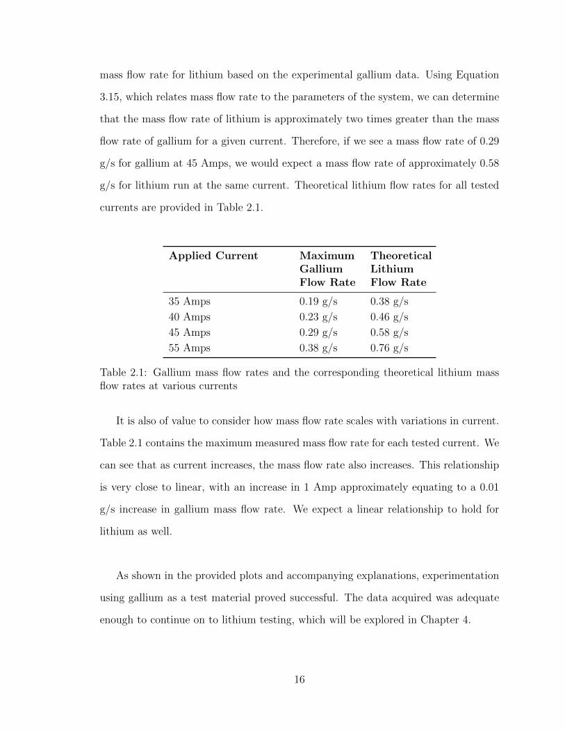
mass flow rate for lithium based on the experimental gallium data. Using Equation

3.15, which relates mass flow rate to the parameters of the system, we can determine

that the mass flow rate of lithium is approximately two times greater than the mass

flow rate of gallium for a given current. Therefore, if we see a mass flow rate of 0.29

g/s for gallium at 45 Amps, we would expect a mass flow rate of approximately 0.58

g/s for lithium run at the same current. Theoretical lithium flow rates for all tested

currents are provided in Table 2.1.

Applied Current MaximumGalliumFlow Rate

TheoreticalLithiumFlow Rate

35 Amps 0.19 g/s 0.38 g/s

40 Amps 0.23 g/s 0.46 g/s

45 Amps 0.29 g/s 0.58 g/s

55 Amps 0.38 g/s 0.76 g/s

Table 2.1: Gallium mass flow rates and the corresponding theoretical lithium massflow rates at various currents

It is also of value to consider how mass flow rate scales with variations in current.

Table 2.1 contains the maximum measured mass flow rate for each tested current. We

can see that as current increases, the mass flow rate also increases. This relationship

is very close to linear, with an increase in 1 Amp approximately equating to a 0.01

g/s increase in gallium mass flow rate. We expect a linear relationship to hold for

lithium as well.

As shown in the provided plots and accompanying explanations, experimentation

using gallium as a test material proved successful. The data acquired was adequate

enough to continue on to lithium testing, which will be explored in Chapter 4.

16

Chapter 3

Concept and Testing of Induction

Probe Mass Flow Control

3.1 Need for Mass Flow Control

The ability to accurately determine mass flow rate in the EM pump system is vital to

the proper functioning of the LiLFA. The applied magnetic field utilized by the pump

is kept constant throughout operation. Therefore, the only way to vary flow rate is

by altering the current in the system. By accurately mapping the applied current to

a measured mass flow rate during testing, it is possible to precisely control the rate

at which lithium propellant is fed to the thruster during firings. Although, theoreti-

cally, mass flow rate and corresponding current can be determined mathematically, as

described in Section 3.2, past experimental results differ significantly from expected

values. Therefore, it is necessary that a mass flow meter be implemented in order to

accurately measure flow resulting from a given applied current.

17

3.2 Mass Flow Rate Derivation

We wish to obtain an equation relating mass flow rate to the parameters of the system.

To begin this derivation, we start with the basic Bernoulli equation, equating the

pressure required to pump the lithium to the hydrostatic elevation pressure and the

dynamic pressure, respectively [9]:

P = ρgh+1

2ρv2 (3.1)

where P = pressure, ρ = lithium density, g = acceleration due to gravity, h = height

of the lithium column in the reservoir, and v = fluid velocity.

Since we are dealing with fluid flow through pipes, it is also important to consider

geometric losses that result from bends, etc.:

4P =ρv2

2k (3.2)

where k = geometric loss coefficient.

It is also necessary to include frictional losses from pipe-flow resistance based off

of the Darcy-Weisbach equation [10]:

4P =fL

D

ρv2

2(3.3)

where f = friction factor, L = tubing length, and D = tubing diameter.

Combining 3.1, 3.2, and 3.3, we can obtain a complete equation for the pressure

needed:

18

P = ρgh+ρv2

2+ρv2

2k +

fL

D

ρv2

2(3.4)

P = ρgh+ρv2

2

(1 + k +

fL

D

)(3.5)

Based on the low flow rates that the feed system operates at, we can safely assume

that the flow in the tubing is laminar. The laminar friction factor f is a function of

Reynold’s number based on the Hagen-Poiseuille equation. For a laminar flow, this

relation is given by 64Re

= 64µρvD

. Plugging into equation 3.5, our new relationship is:

P = ρgh+ρv2

2

(1 + k +

64µL

ρvD2

)(3.6)

where µ = viscosity.

Markusic et al. [8] provide a relation between pressure and current when consid-

ering the Lorentz force. For a DC conduction pump, this relation is:

P =IB

s(3.7)

Where I = current, B = magnetic field strength, and s = magnet separation distance.

For simplicity, we can say that Bs = B/s.

Plugging Markusic et al.’s relation into 3.6, we can obtain an equation for current

as a function of the system’s parameters:

I =1

Bs

[ρgh+

ρv2

2

(1 + k +

64µL

ρvD2

)](3.8)

Rearranging this equation, we get:

ρgh+ρv2

2

(1 + k +

64µL

ρvD2

)− IBs = 0 (3.9)

19

ρv2

2(1 + k) +

ρv2

2

64µL

ρvD2+ (ρgh− IBs) = 0 (3.10)

ρ

2(1 + k)v2 +

32Lµ

D2v + (ρgh− IBs) = 0 (3.11)

By solving the quadratic equation, we can reach an expression for fluid velocity,

v, as a function of the system’s parameters:

v =

−32LµD2 +

√(32LµD2 )2 + 2ρ(1 + k)(IBs − ρgh)

ρ(1 + k)(3.12)

We can relate fluid velocity, v, to mass flow rate, assuming that the flow is of

uniform density, by:

m = ρvA =ρvπD2

4(3.13)

v =4m

ρπD2(3.14)

where m = mass flow rate and A = cross sectional area of the tubing.

If we substitute this relation between m and v back into equation 3.12, we obtain

a final relation for m as a function of the system’s parameters:

m =π(−32Lµ+

√(32Lµ)2 + 2ρ(1 + k)(IBs − ρgh)D4

)4(1 + k)

(3.15)

This relationship is useful for assessing the uncertainty in the feed system, which

will be further explored in Chapter 5.

3.3 Prior Setup Using Plumb Bob Method

The previous system utilized a steel-tipped plumb bob attached to a piston arm in

order to measure mass flow rate. Using LabVIEW programming, the apparatus was

20

lowered incrementally over the surface of the liquid metal reservoir until making con-

tact with the gallium test material. This completed a circuit, signaling to the control

system to stop the plumb bob’s movement and record its height. By monitoring the

change in vertical distance of the plumb bob, in conjunction with the accumulation

of mass on the Sartorius AY303 scale at the system exit point, the flow rate could be

calculated as a function of time.

After several tests of the plumb bob system and a thorough analysis of the output

data files, it was determined that the plumb bob system was too faulty to garner

accurate mass flow rate results within the 5 mg/s or less accuracy range desired. The

margin of error was roughly 20 percent or greater, which is too high for a sufficient feed

system. While the plumb bob itself worked well, the system could not take frequent

samples due to the wetting of gallium to the tip of the plumb bob. Therefore, it was

determined that the plumb bob method needed to be replaced with a more accurate

sensor.

3.4 Use of an Induction Probe

In place of the plumb bob, an induction probe was selected as a better flow meter

alternative. This is preferred over the plumb bob apparatus due to its ability to

measure reservoir height change without contact. A non-contact system is especially

useful for final testing with lithium due to its reactive properties. The probe functions

by outputting a voltage based on its proximity to a metal surface. By attaching the

probe to the piston arm from the previous feed system, it can be lowered incrementally

over the liquid metal reservoir and the position can be tracked. Depending on the

distance between the probe and the metal, the probe is able to measure a certain

voltage. Knowing the position of the probe and the distance from the lithium surface

21

based on this voltage, mass flow rate can be calculated from the change in height of

the lithium column. As determined in Section 2.5, we expect that the mass flow rate

will decrease roughly linearly as the pressure head decreases.


To test the probe, it was placed within the system described in Section 2.3. The

probe was attached to the piston arm from the previous feed system, where it could

be lowered with control over the liquid metal reservoir. The voltage from the probe

is read by the LabVIEW program, which can then determine whether or not to lower

the probe based on the value of the reading compared to a certain inputted threshold

value. For this experiment, the probe is considered to be a measurable distance from

the lithium surface when the voltage value drops below 10 volts. This wide threshold

is used to ensure no contact with the liquid lithium, which will damage the apparatus.

The exit of the feed system is placed over a container on the scale. This allows us to

compare mass flow rates based on height change to the amount of mass accumulated

on the scale.

3.6 Procedure

Similar to the J ×B pump test procedure detailed in Section 2.4, the entire system

is first heated to a minimum of 30◦C using a series of band heaters and heat gun

application. The solid gallium is melted in a separate container using a heat gun and

then poured into the inlet reservoir. After the system is primed, the surface of the

liquid gallium is determined by lowering the probe over the reservoir until the voltage

reading drops below the 10 volts threshold. This is considered the starting height

for the probe. The power supply is then turned on. Using LabVIEW, the input

current can be set to a range of values. For this experiment, the current is set to the

22

maximum of 70 Amps in order to test the full capacity of the pump. Data values for

mass, time, current and voltage are recorded in an output file to be later analyzed. A

calibration was completed in order to understand how voltage corresponds to probe

position. The experiment was repeated numerous times in order to ensure robustness

of the measurement system.


It was determined that the induction probe is a suitable alternative to the plumb

bob methodology for mass flow rate measurement. The probe was able to accurately

detect the surface of the liquid gallium within the reservoir. From the recorded data,

we can analyze how probe position affects the output voltage. Figure 3.1 provides a

calibration of the probe data, showing voltage as a function of the probe’s position.

Figure 3.1: Voltage as a function of probe position

23

We can see that at far distances, the voltage reading is relatively high, ranging

from 8.5 volts to the maximum of 10 volts. At approximately 27 millimeters from the

liquid surface, the voltage sharply decreases. After this point, the voltage decreases

roughly linearly at a rate of 10 V/cm as the probe is moved closer to the gallium. At

this distance, the probe is considered to be a measurable distance from the surface.

This acts at the starting point for all mass flow rate measurements. As the liquid

gallium flows through the system, we aim to maintain this distance over the liquid

surface by incrementally lowering the probe and monitoring the output voltage.

24

Chapter 4

Testing with Lithium


Once sufficient mass flow rates were achieved using gallium and the induction probe

was deemed a suitable measurement system, experimentation transitioned to using

lithium as a propellant. This necessitated the construction of a new feed system in

order to accommodate for the corrosive and reactive properties of lithium. Based

on experiments completed using gallium, several changes were made to the previous

feed system in order to ensure robustness when testing with lithium. This primarily

includes:

1) The inclusion of overlapping, redundant heating systems in order to prevent

lithium freezing throughout the flow

2) The design of a spring-controlled system to vacuum seal the reservoir chamber

with the induction probe contained inside

3) The insertion of thermocouples throughout the system to accurately monitor

temperature throughout the flow

25

A schematic of the system is provided in Figure 4.1, while various views of the

system are shown in Figures 4.2 and 4.3. In the new setup, the liquid lithium is

first stored in the reservoir under vacuum. The reservoir measures 7-3/4 inches in

height and 1-3/8 inches in diameter. The propellant then travels through the steel

reservoir line (inner diameter of .085 inch) to the J×B pump, shown in Figure 4.4.

The current and magnetic field generated by the power supply and high-temperature

grade Samarium-Cobalt magnets, respectively, generate a Lorentz body force. The

pressure applied at this point acts to pump the lithium through the tubing and to

the cylindrical spiral. The propellant is pumped up the spiral to the cathode of the

thruster. In total, the tubing measures approximately 6 feet in length for this setup.

The entire system is heated with a series of copper blocks and cartridge heaters. For

these initial experimental purposes, the exit of the feed system is positioned over a

Sartorius AY303 scale in order to make mass measurements for flow rate calculations.

Figure 4.1: Schematic of the experimental setup for lithium

26

Figure 4.2: View of the lithium setup from outside of the tank

Figure 4.3: Close-up view of the lithium setup

27

Figure 4.4: Close-up view of the J×B pump within the lithium setup

4.2 Procedure

Solid lithium is first loaded into the reservoir chamber and then the system is vacuum

sealed and heated. LabVIEW is used to monitor the increase in temperature within

the reservoir and to determine whether or not a phase change has occurred in the solid

lithium. After the lithium has become liquid, temperature increases downstream in

the feed system are monitored to ensure that lithium freezes do not occur. Operating

temperatures of the system typically range from 200 - 250 ◦C. Once the entire system

is sufficiently heated and the pump is primed, the induction probe is lowered until

it identifies the surface of the lithium. This occurs when the probe voltage reading

drops below 10 volts. The power supply is then turned on and a desired current

is applied. The current is varied depending on the mass flow rate that needs to be

achieved. The LabVIEW program then monitors the mass flow rate of the lithium

through the system and records the data to an output file. In the case where no

mass flow is being read by the program, argon, which does not react with lithium,

can be pumped through the system in order to push the lithium through. This can

28

help determine whether the fault is an error with the pumps operation or if there is

lithium frozen downstream in the line.


At this point in time, obtaining accurate mass flow rate measurements of the lithium

system is proving to be somewhat faulty. While the heating mechanism works well

and the pump is able to be primed, the system is running into difficulty with the

pumping process itself. The issues lies in the phenomenon of vapor lock. The gravity

well is insufficient to back fill the pump with lithium due to the surface tension of the

liquid. This was partially solved by altering the diameter of the tubing to 1/4-inch

between the reservoir and the pump. However, extra back pressure using the argon

line is still required. Possibly explanations are:

1) the pump is being operated at too high of a current or magnetic field strength,

meaning that it is pumping the lithium too hard and creating a vapor lock

2) lithium is reacting with the atmosphere at the exit point and forming a crust,

thus requiring more pressure to pump further lithium through

Further experimentation will be required in order to determine how to solve this

issue and to ensure robustness of the feed system with lithium.

29

Chapter 5

Error Analysis

5.1 Error Derivation

Based on the complexity of the J×B pump feed system, it is of interest to determine

the levels of uncertainty associated with mass flow rate calculations. The mass flow

rate is affected by a number of parameters, including the geometric loss coefficient

k, viscosity µ, tubing length L, density ρ, current I, magnetic field strength Bs,

acceleration due to gravity g, height h, and diameter D.

However, we also do not know the individual uncertainties in these dependent

variables. It is therefore necessary to estimate the error in each measured quantity.

We can then combine the standard deviations, σx, of the individual measurements

to estimate the uncertainty in our final result for mass flow rate.

Bevington and Robinson derive the following formula for error propagation, while

assuming that x = f(u, v, ...) [11]:

σ2x = σ2

u

(∂x

∂u

)2

+ σ2v

(∂x

∂v

)2

+ ... (5.1)

30

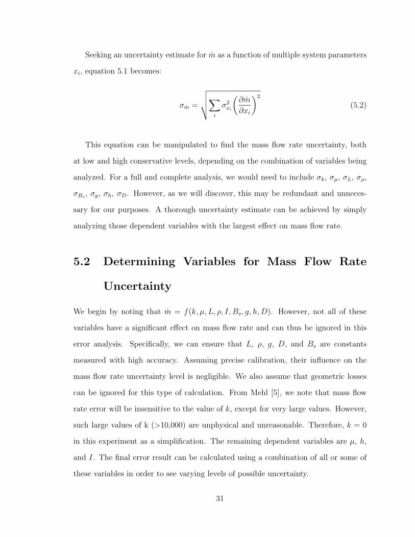
Seeking an uncertainty estimate for m as a function of multiple system parameters

xi, equation 5.1 becomes:

σm =

√√√√∑i

σ2xi

(∂m

∂xi

)2

(5.2)

This equation can be manipulated to find the mass flow rate uncertainty, both

at low and high conservative levels, depending on the combination of variables being

analyzed. For a full and complete analysis, we would need to include σk, σµ, σL, σρ,

σBs , σg, σh, σD. However, as we will discover, this may be redundant and unneces-

sary for our purposes. A thorough uncertainty estimate can be achieved by simply

analyzing those dependent variables with the largest effect on mass flow rate.

5.2 Determining Variables for Mass Flow Rate

Uncertainty

We begin by noting that m = f(k, µ, L, ρ, I, Bs, g, h,D). However, not all of these

variables have a significant effect on mass flow rate and can thus be ignored in this

error analysis. Specifically, we can ensure that L, ρ, g, D, and Bs are constants

measured with high accuracy. Assuming precise calibration, their influence on the

mass flow rate uncertainty level is negligible. We also assume that geometric losses

can be ignored for this type of calculation. From Mehl [5], we note that mass flow

rate error will be insensitive to the value of k, except for very large values. However,

such large values of k (>10,000) are unphysical and unreasonable. Therefore, k = 0

in this experiment as a simplification. The remaining dependent variables are µ, h,

and I. The final error result can be calculated using a combination of all or some of

these variables in order to see varying levels of possible uncertainty.

31

5.3 Contribution of Viscosity, Height, and Current

to Mass Flow Rate Uncertainty

To gain a fully encompassing estimate of mass flow rate error, we seek to include

individual uncertainties for all three significant dependent variables: µ, h, and I.

σm =

√σ2µ

(∂m

∂µ

)2

+ σ2h

(∂m

∂h

)2

+ σ2I

(∂m

∂I

)2

(5.3)

Ascertaining the standard deviations for µ and I are simple; σµ is provided by

Mehl [5] as 2% and σI is provided in the power supply manual as 3% for running in

current control mode. We can complete a separate analysis for σh.

We know that the voltage from the induction probe read by the LabVIEW

system is directly related to the column height. By completing a calibration, we

can obtain an equation for voltage as a function of probe position. We can find a

best fit function for the experimental position data, which is a cubic function in this

case. We can then plot the actual measured position versus voltage and compare

this to the idealized fit plot. From this, we can ascertain an average standard devi-

ation in probe position. When this analysis is completed, it is found that σp = 0.0134.

Since the voltage reading is a direct result of the probe’s position in relation to

the liquid metal surface, we can assume that the standard deviation in probe position

and reservoir height are approximately the same for our purposes, or σp = σh = .0134.

A source of uncertainty associated with this assumption includes the presence of

vibrational disturbances in the liquid lithium, which could lead to inaccurate height

readings. However, we can neglect such errors since data measurements are averaged

over timescales much greater than the period of any oscillation in the system. Other

32

sources of error might include accumulation of solid lithium in certain sections of the

reservoir. This can be avoided by properly heating the system to ensure a complete

liquid phase change.

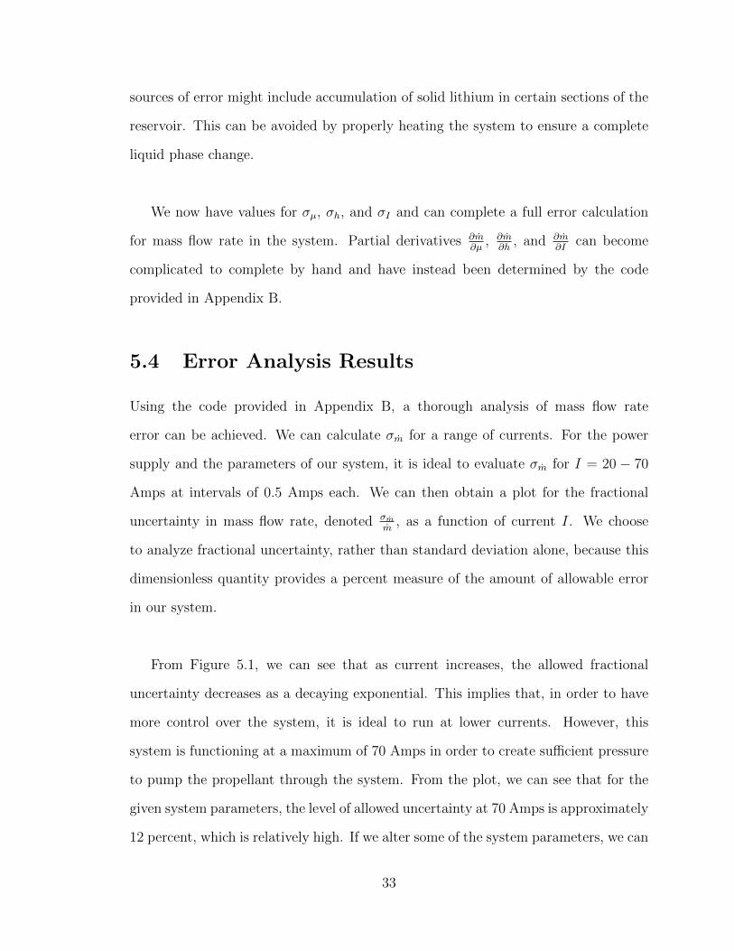
We now have values for σµ, σh, and σI and can complete a full error calculation

for mass flow rate in the system. Partial derivatives ∂m∂µ

, ∂m∂h

, and ∂m∂I

can become

complicated to complete by hand and have instead been determined by the code

provided in Appendix B.

5.4 Error Analysis Results

Using the code provided in Appendix B, a thorough analysis of mass flow rate

error can be achieved. We can calculate σm for a range of currents. For the power

supply and the parameters of our system, it is ideal to evaluate σm for I = 20 − 70

Amps at intervals of 0.5 Amps each. We can then obtain a plot for the fractional

uncertainty in mass flow rate, denoted σmm

, as a function of current I. We choose

to analyze fractional uncertainty, rather than standard deviation alone, because this

dimensionless quantity provides a percent measure of the amount of allowable error

in our system.

From Figure 5.1, we can see that as current increases, the allowed fractional

uncertainty decreases as a decaying exponential. This implies that, in order to have

more control over the system, it is ideal to run at lower currents. However, this

system is functioning at a maximum of 70 Amps in order to create sufficient pressure

to pump the propellant through the system. From the plot, we can see that for the

given system parameters, the level of allowed uncertainty at 70 Amps is approximately

12 percent, which is relatively high. If we alter some of the system parameters, we can

33

Figure 5.1: Fractional uncertainty in mass flow as a function of current

see how this affects allowed uncertainty. For example, tubing length proves to have a

significant effect upon the system. Figure 5.2 shows the allowed fractional uncertainty

in mass flow rate as a function of current for a system measuring half the length of our

setup. By decreasing tubing length, the allowed fractional uncertainty at 70 Amps

decreases to about 6 percent. Based on Equation 3.3, this makes intuitive sense. A

decrease in tubing length will decrease the effect of frictional losses throughout the

system, and thus allow for less control over the system. Therefore, we can conclude

that more friction, and, thus, longer tube length, is ideal for this system. With

greater friction, the mass flow rate for a given current will be lower and, therefore,

more controllable. Another alternative to consider is decreasing the tubing diameter,

which would also increase frictional losses, as well as flow velocity, which contributes

to dynamic pressure. If we increase frictional losses and dynamic pressure, more

34

current will be required to generate enough pressure to push the lithium through the

system.

Figure 5.2: Fractional uncertainty in mass flow as a function of current, assuming ashorter tubing length

35

Chapter 6

Conclusion

6.1 Conclusion and Remarks

Throughout the course of this experimentation, it was determined that a J×B pump

is a suitable alternative for the LiLFA feed system. Through preliminary testing

using gallium, we can see that measurable mass flow rates can be achieved and con-

trolled based on applied current. When converting these experimental flow rates to

theoretical values for lithium, we propose that we can produce sufficient flow in a

lithium-based system. The induction probe measurement system proved to operate

successfully using both gallium and lithium. While proving faulty in some regards,

the transition to a lithium propellant system seems promising based on early work.

6.2 Future Work

Before the LiLFA can be considered a viable proposal for future space missions,

it is vital to prove the robustness of the feed system using lithium. Based on the

complications with the current system, the most pertinent step is determining how to

solve the vapor lock issue, which is preventing the pump from functioning properly.

36

Possible future work to consider is:

1) Running the system at various currents to map changing mass flow rates. This

will allow for a test of the feedback loop, which will ultimately provide a constant

mass flow rate despite the changing potential.

2) Analyze the data to determine if desired flow rates and precisions can be

achieved using this methodology. If not, implementing a duty cycle-like method

for the power supply could be an alternative. If the system works best between two

specific currents, the power supply can toggle rapidly between them in order to get

the desired effect.

37

Appendix A

Mass Flow Rate of Gallium withMATLAB - MFR45Agallium.m

clear all

[mass time timeave mfr current voltage piston] ...

= textread(’20151228_ForwardJ=45A.dat’,’%f%f%f%f%f%f%f’,’headerlines’,1);

x = time;

y = mass;

pts = 10; % number of drops to average over

TotT = length(x);

TotM = length(y);

% create mass and time vectors

for i=1:TotM

if i==1

m(i) = 0; % fill with zeros

t(i) = 0;

elseif i<TotM

diff = y(i)-y(i-1);

if diff > .3

m(i) = y(i);

t(i) = x(i);

else m(i) = 0;

t(i) = 0;

end

else m(i) = 0;

t(i) = 0;

end

end

38

%remove zeros from data

m(m==0) = [];

l = length(m);

t(t==0) = [];

% mass vs. time - raw data

figure(1)

plot(t(1:l),m(1:l))

xlabel(’time’)

ylabel(’mass’)

title(’Mass vs. Time’)

% mass vs. time, split into 5 trials

figure(2)

plot(t(1:82),m(4:85))

hold on

plot(t(1:100),m(86:185))

plot(t(1:93),m(186:278))

plot(t(1:97),m(279:375))

plot(t(1:90),m(376:465))

xlabel(’Time (s)’)

ylabel(’Mass (g)’)


% finding a best fit average line for all 5 trials

% first, find coefficients of each trial best fit line

fa = polyfit(t(1:82),m(4:85),1)

fb = polyfit(t(1:100),m(86:185),1)

fc = polyfit(t(1:93),m(186:278),1)

fd = polyfit(t(1:97),m(279:375),1)

fe = polyfit(t(1:90),m(376:465),1)

% store coefficients

p1 = [fa(1),fb(1),fc(1),fd(1),fe(1)]

p2 = [fa(2),fb(2),fc(2),fd(2),fe(2)]

% find average slope and intercept

ave_p1 = mean(p1)

ave_p2 = mean(p2)

% create linear model for average slope and intercept

f_lin = fittype(’a*x+b’)

ave_lin = cfit(f_lin,ave_p1,ave_p2)

%finding a best fit average parabola for all 5 trials

39

% first, find coefficients of each trial’s best fit parabolic curve

fa_p = polyfit(t(1:82),m(4:85),2)

fb_p = polyfit(t(1:100),m(86:185),2)

fc_p = polyfit(t(1:93),m(186:278),2)

fd_p = polyfit(t(1:97),m(279:375),2)

fe_p = polyfit(t(1:90),m(376:465),2)


p1_p = [fa_p(1),fb_p(1),fc_p(1),fd_p(1),fe_p(1)]



% find average coefficients

ave_p1_p = mean(p1_p)



% create parabolic model for average coefficients

f_para = fittype(’a*x^2+b*x+c’)

ave_para = cfit(f_para,ave_p1_p,ave_p2_p,ave_p3_p)

% mass vs time for 5 trials with best fit linear average

figure(3)

plot(t(1:82),m(4:85),’g’)

hold on

plot(t(1:100),m(86:185),’c’)

plot(t(1:93),m(186:278),’r’)

plot(t(1:97),m(279:375),’m’)

plot(t(1:90),m(376:465),’b’)

plot(ave_lin,’-.’)




legend(’Trial 1’,’Trial 2’,’Trial 3’,’Trial 4’,’Trial 5’,’Average’,...

’Location’,’southeast’)

% mass vs time for 5 trials with best fit parabolic curve average

figure(4)

plot(t(1:82),m(4:85),’g’)

hold on

plot(t(1:100),m(86:185),’c’)

plot(t(1:93),m(186:278),’r’)

plot(t(1:97),m(279:375),’m’)

plot(t(1:90),m(376:465),’b’)

plot(ave_para,’-.’)

40





’Location’,’southeast’)

% find average mass and mass flow rate (sl)

for i=pts:l

numer(i) = m(i)-m(i-pts+1);

denom(i) = t(i)-t(i-pts+1);

sl(i) = numer(i)/denom(i);

avemass(i) = m(i-pts+1)+numer(i)/2;

end

% remove values for when gallium is re-poured into reservoir

l3 = length(avemass)

for i=1:l3

if i==1

run(1) = 0;

elseif avemass(i) > avemass(i-1);

run(i) = avemass(i);

end

end

% plot dm/dt versus mass averaging over 10 points (raw data)

figure(5)

plot(run(14:85),sl(14:85))

xlabel(’mass’)

ylabel(’dm/dt’)

hold on

plot(run(96:185),sl(96:185))

plot(run(196:278),sl(196:278))

plot(run(289:375),sl(289:375))

plot(run(386:465),sl(386:465))

legend(’One’,’Two’,’Three’,’Four’,’Five’,’Location’,’southwest’)

title(’dm/dt vs. mass - separate runs’)

%plot best fit line for each trial run

run_fit = run’;

sl_fit = sl’;

% find best fit for each trial

f1 = fit(run_fit(14:85),sl_fit(14:85),’poly1’)

41





% find coefficients of each trial’s best fit line

f1_l = polyfit(run_fit(14:85),sl_fit(14:85),1)






slope = [f1_l(1),f2_l(1),f3_l(1),f4_l(1),f5_l(1)]

intercept = [f1_l(2),f2_l(2),f3_l(2),f4_l(2),f5_l(2)]

% find average slope and intercept

ave_intercept = mean(intercept)

ave_slope = mean(slope)

% create linear model for average slope and intercept

f = fittype(’a*x+b’)

ave = cfit(f,ave_slope,ave_intercept)

% plot best fit lines for each trial run and average fit line

figure(6)

plot(f1,’g’)

hold on

plot(f2,’c’)

plot(f3,’r’)

plot(f4,’m’)

plot(f5,’b’)

plot(ave,’-.’)


’Location’,’southwest’)

title(’Mass Flow Rate vs. Mass - 45A’)

xlabel(’Mass (g)’)

ylabel(’Mass Flow Rate (g/s)’)

% plot average fit line over raw data

figure(7)

plot(run(14:85),sl(14:85),’g’)

hold on

plot(run(96:185),sl(96:185),’c’)

plot(run(196:278),sl(196:278),’r’)

42

plot(run(289:375),sl(289:375),’m’)

plot(run(386:465),sl(386:465),’b’)

plot(ave,’-.’)


’Location’,’southwest’)

title(’Mass Flow Rate vs. Mass - 45A’)

xlabel(’Mass (g)’)

ylabel(’Mass Flow Rate (g/s)’)

43

Appendix B

Uncertainty Analysis withMATLAB - LiLFAerror.m

clear all

mu = 6e-4; % at operating temperature (Pa-s)

k = 0; % geometric losses coefficient - ignore

L = 1.8288; % m

ro = 512; % density of lithium at operating temperature (kg/m^3)

I = 70; % current (Amps)

Bs = 21; % magnetic field strength (T/m)

g = 9.81; % acceleration due to gravity (m/s2)

h = .1; % height (m)

D = .002159; % diameter of tubing (m)

mdot_val = (pi/(4*(1+k)))*(-32*mu*L + sqrt((32*mu*L)^2+2*ro*(1+k)*...

(I*Bs-ro*g*h)*D^4))

% ERROR IN MASS FLOW BASED ON CURRENT, VISCOSITY, AND HEIGHT UNCERTAINTY

% symbolic variables

syms c rho B_s grav height len dia visc massflow

% mass flow rate from Equation 3.15

mdot = (pi/(4*(1+k)))*(-32*visc*len + sqrt((32*visc*len)^2+2*rho*(1+k)*...

(c*B_s-rho*grav*height)*dia^4));

% partial differentials

dmdot_dI = diff(mdot,c);

dmdot_dh = diff(mdot,height);

dmdot_dmu = diff(mdot,visc);

% loop over currents

44

i = 1;

for I_vals = 20:.5:300;

%sub in values

dmdot_dI_val = subs(dmdot_dI,[B_s,dia,rho,len,visc,height,c,grav],...

[Bs,D,ro,L,mu,h,I_vals,g]);

dmdot_dh_val = subs(dmdot_dh,[B_s,dia,rho,len,visc,height,c,grav],...


dmdot_dmu_val = subs(dmdot_dmu,[B_s,dia,rho,len,visc,height,c,grav],...


sigma_I = .03; % From Acopian manual

sigma_h = .0134; %from LabVIEW experiment

sigma_mu = .02; % from Mehl thesis

sigma_mdot = sqrt(dmdot_dI_val^2*sigma_I^2 + dmdot_dh_val^2*sigma_h^2 +...

dmdot_dmu_val^2*sigma_mu^2);

mdot_sub = subs(mdot,[B_s,dia,rho,len,visc,height,c,grav],...


% allowed fractional uncertainty

sigmamdot_mdot(i) = sigma_mdot/mdot_sub;

i = i+1;

end

% plot fractional uncertainty versus current

I_vals = 20:.5:300;

figure(1)

plot(I_vals,sigmamdot_mdot)

xlabel(’Current (Amps)’)

ylabel(’Fractional Uncertainity - Mass Flow (unitless)’)

title(’Fractional Uncertainty in Mass Flow vs. Current’)

45

Bibliography

[1] NASA Glenn Research Center. Ideal Rocket Equation. https://

spaceflightsystems.grc.nasa.gov/education/rocket/rktpow.html, Octo-ber 2015.

[2] National Aeronautic and Space Administration. Rocket Performance Parametersand Units. http://history.nasa.gov/SP-4404/app-b8.html.

[3] Robert G. Jahn. Physics of Electric Propulsion, chapter 1. Courier Corporation,2012.

[4] Princeton University Electric Propulsion and Plasma Dynamics Laboratory.Lithium Lorentz Force Accelerator. http://alfven.princeton.edu/projects/LiLFA.htm, 2015.

[5] Jeremy Mehl. Design and Testing of a Propellant Feed System for the LithiumLorentz Force Accelerator, April 2015.

[6] Lenntech. Chemical properties of gallium. http://www.lenntech.com/

periodic/elements/ga.htm, 2016.

[7] Element Properties. Electrical Conductivity of the Elements. http://

periodictable.com/Properties/A/ElectricalConductivity.an.html.

[8] Thomas E. Markusic, Kurt A. Polzin, and Amado Dehoyos. Electromagneticpumps for conductive-propellant feed systems. In 29th International ElectricPropulsion Conference, 2005.

[9] Princeton University. Bernoulli’s Equation. https://www.princeton.edu/

~asmits/Bicycle_web/Bernoulli.html.

[10] Glenn Brown. The Darcy-Weisbach Equation. https://bae.okstate.edu/

faculty-sites/Darcy/DarcyWeisbach/Darcy-WeisbachEq.htm, June 2000.

[11] Philip R. Bevington and D. Keith Robinson. Data Reduction and Error Analysisfor the Physical Sciences. Wiley, 2008.

46

Control and Analysis of a JxB Pump Propellant Feed System ...

Documents

Transcript of Control and Analysis of a JxB Pump Propellant Feed System ...