CONTROL ACTUATION SYSTEMS AND SEEKER …kullanılabilecek bulanık mantık denetleyicisi...
138
CONTROL ACTUATION SYSTEMS AND SEEKER UNITS OF AN AIR-TO-SURFACE GUIDED MUNITION A THESIS SUBMITTED TO THE GRADUATE SCHOOL OF NATURAL AND APPLIED SCIENCES OF THE MIDDLE EAST TECHNICAL UNIVERSITY BY ELZEM AKKAL IN PARTIAL FULFILMENT OF THE REQUIREMENTS FOR THE DEGREE OF MASTER OF SCIENCE IN THE DEPARTMENT OF ELECTRICAL AND ELECTRONICS ENGINEERING DECEMBER 2003
Transcript of CONTROL ACTUATION SYSTEMS AND SEEKER …kullanılabilecek bulanık mantık denetleyicisi...

CONTROL ACTUATION SYSTEMS AND SEEKER UNITS OF AN
AIR-TO-SURFACE GUIDED MUNITION
A THESIS SUBMITTED TO THE GRADUATE SCHOOL OF NATURAL AND APPLIED SCIENCES
OF THE MIDDLE EAST TECHNICAL UNIVERSITY
BY
ELZEM AKKAL
IN PARTIAL FULFILMENT OF THE REQUIREMENTS FOR THE DEGREE
OF
MASTER OF SCIENCE
IN
THE DEPARTMENT OF ELECTRICAL AND ELECTRONICS ENGINEERING
DECEMBER 2003

Approval of the Graduate School of Natural and Applied Sciences
Prof. Dr. Canan Özgen Director I certify that this thesis satisfies all the requirements as a thesis for the degree of Master of Science
Prof. Dr. Mübeccel Demirekler Head of the Department This is to certify that we have read this thesis and that in our opinion it is fully adequate, in scope and quality, as a thesis for the degree of Master of Science.
Prof. Dr. Kemal Leblebicioğlu
Supervisor
Examining Committee Members
Prof. Dr. Kemal Özgören
Prof. Dr Kemal Leblebicioğlu
Prof. Dr. Uğur Halıcı
Assoc. Prof. Dr. Ozan Tekinalp
M. Sc. Özgür Ateşoğlu
iii
ABSTRACT
CONTROL ACTUATION SYSTEMS AND SEEKER UNITS OF AN
AIR-TO-SURFACE GUIDED MUNITION
Akkal, Elzem
M.S., Department of Electrical and Electronics Engineering
Supervisor : Prof. Dr. Kemal Leblebicioğlu
December 2003, 120 pages
This thesis proposes a modification to an air to surface guided munition (ASGM)
from bang-bang control scheme to continuous control scheme with a little cost. In
this respect, time domain system identification analysis is applied to the control
actuation system (CAS) of ASGM in order to obtain its mathematical model and
controller is designed using pulse width modulation technique. With this
modification, canards would be deflected as much as it is commanded to. Seeker
signals are also post-processed to obtain the angle between the velocity vector and
target line of sight vector. The seeker is modeled using an artificial neural network.
Non-linear flight simulation model is built using MATLAB Simulink and obtained
seeker and CAS models are integrated to the whole flight simulation model having

iv
6 degrees of freedom. As a flight control unit, fuzzy logic controller is designed,
which is a suitable choice if an inertial measurement sensor will not be mounted on
the munition. Finally, simulation studies are carried out in order to compare the
performance of the “ASGM” and “improved ASGM” and the superiority of the
new design is demonstrated.
Keywords: System Identification, Laser Seeker, Control Actuation System,
Artificial Neural Network, Pulse Width Modulation, Fuzzy Logic Control.
v
ÖZ
HAVADAN KARAYA GÜDÜMLÜ BİR MÜHİMMAT İÇİN KONTROL
TAHRİK SİSTEMİ VE ARAYICI BİRİMLERİ
Akkal, Elzem
Yüksek Lisans, Elektrik-Elektronik Mühendisliği Bölümü
Tez Yöneticisi: Prof. Dr. Kemal Leblebicioğlu
Aralık 2003, 120 sayfa
Bu tez, havadan karaya güdümlü bir mühimmatın (HKGM) az bir maliyetle bang-
bang kontrolden sürekli kontrol uygulamasına geçirilmesi değişikliğini
önermektedir. Bu bağlamda, havadan karaya güdümlü mühimmatın kontrol tahrik
sisteminin matematiksel modelinin oluşturulması için sistem tanımlama çalışmaları
uygulanmıştır ve darbe genişliği modulasyonu tekniği kullanılarak kontrol
algoritmaları tasarlanmıştır. Bu değişiklikle kanatçıklar istenilen açılara
getirilebileceklerdir. Hız vektörüyle görüş hattı vektörünün oluşturduları açıyı elde
edebilmek için arayıcı sinyalleri de işlenmiştir. Arayıcı yapay sinir ağları
kullanılarak modellenmiştir. Doğrusal olmayan uçuş modeli MATLAB Simulink

vi
kullanılarak oluşturulmuş, ve kontrol tahrik sistemi modeliyle arayıcı modeli de 6
serbestlik dereceli uçuş simülasyon modeline entegre edilmiştir. Uçuş denetleyicisi
olarak da, mühimmata ataletsel ölçüm sensörleri takılmayacaksa da
kullanılabilecek bulanık mantık denetleyicisi tasarlanmıştır. Son olarak da,
“HKGM” ile “geliştirilen HKGM”nin performanslarını karşılaştırabilmek için,
simülasyon çalışmaları yapılmış ve yeni tasarımın üstünlüğü gösterilmiştir.
Anahtar Kelimeler: Sistem Tanımlama, Lazer Arayıcı, Kontrol Tahrik Sistemi,
Yapay Sinir Ağları, Darbe Genişlik Modulasyonu, Bulanık Mantık Denetleyicisi.

vii
Dedicated to the most important person
I could ever have in my life,
Bülent Semerci...

viii
ACKNOWLEDGEMENTS
I would like to express my sincere thanks and appreciation to my supervisor Prof.
Dr. Kemal LEBLEBİCİOĞLU for his support, guidance and understanding during
the preparation of this thesis.
I would like to acknowledge the manager of Navigation and Guidance Systems
Design group, Dr. Murat EREN, for his support throughout this study.
Special thanks to my mother Çiğdem, my father Bülent and my sister Ahugün for
their love, support and understanding at all stages of my life.
I also wish to thank to all my colleagues at ASELSAN-MGEO-SGSTM, especially
Özgür ATEŞOĞLU, Yıldız LALETAŞ and D.R. Levent GÜNER for their support
and motivation.
Last, but definitely not the least, I am very grateful to Bülent SEMERCİ for his
love, patience and understanding during this study.
ix
TABLE OF CONTENTS
ABSTRACT............................................................................................................. iii
ÖZ ............................................................................................................................. v
ACKNOWLEDGEMENTS ...................................................................................viii
TABLE OF CONTENTS......................................................................................... ix
LIST OF TABLES .................................................................................................. xii
LIST OF FIGURES................................................................................................xiii
NOMENCLATURE.............................................................................................. xvii
CHAPTER
1 INTRODUCTION................................................................................................. 1
1.1 General Information About the ASGM ..................................................................................... 1
1.2 About Thesis .............................................................................................................................. 3
2 MISSILE EQUATIONS OF MOTION ................................................................ 5
2.1 Introduction ................................................................................................................................ 5
2.2 Development of Equations of Motion ....................................................................................... 5
2.2.1 Reference Axis Systems and Axis Transformations .......................................................... 5
2.2.2 Derivation of Dynamic Equations .................................................................................... 8
2.2.3 Derivation of Kinematic Equations ................................................................................ 12
2.3 Forces and Moments Acting on a Missile ............................................................................... 14
2.3.1 Gravitational Force......................................................................................................... 14
x
2.3.2 Aerodynamic Forces and Moments ................................................................................ 15
3 SYSTEM IDENTIFICATION FOR THE CONTROL ACTUATION SYSTEM
................................................................................................................................. 21
3.1 Introduction .............................................................................................................................. 21
3.2 Control Actuation System Setup.............................................................................................. 22
3.2.1 Description of Control Actuation System ....................................................................... 22
3.2.2 Description of Test Setup ................................................................................................ 25
3.3 MATLAB System Identification Toolbox .............................................................................. 27
3.4 System Identification for CAS................................................................................................. 29
3.4.1 System Identification Using First Scheme ...................................................................... 30
3.4.2 System Identification Using Second Scheme .................................................................. 39
4 CONTROLLER DESIGN WITH PWM FOR CONTROL ACTUATION
SYSTEM ................................................................................................................. 42
4.1 Introduction .............................................................................................................................. 42
4.2 Pulse Width Modulation .......................................................................................................... 43
4.3 Controller with PWM............................................................................................................... 46
4.3.1 Controller for First PWM Scheme.................................................................................. 47
4.3.2 Controller for Second PWM Scheme .............................................................................. 53
5 SEEKER MODEL ............................................................................................... 57
5.1 Introduction .............................................................................................................................. 57
5.2 Relation of the Spot Location with the Error Angle ............................................................... 60
5.3 Estimation of Spot Location .................................................................................................... 61
5.3.1 Artificial Neural Networks .............................................................................................. 63
5.3.2 Determination of Training Data Set ............................................................................... 66
5.4 Results of the Radial Basis Neural Network Model of Seeker ............................................... 68
5.5 Summary .................................................................................................................................. 71
6 OVERALL ASGM MATHEMATICAL MODEL.............................................. 73
xi
6.1 Introduction .............................................................................................................................. 73
6.2 Fuzzy Logic Control for Missile.............................................................................................. 73
6.2.1 What is Fuzzy Logic Control........................................................................................... 73
6.2.2 Description of Designed Fuzzy Logic Control ............................................................... 77
6.3 Integration of CAS and Seeker Models to the Non-linear Flight Model................................ 80
7 SIMULATION STUDIES.................................................................................... 83
7.1 Introduction .............................................................................................................................. 83
7.2 Simulation Scenarios................................................................................................................ 83
7.2.1 Scenario 1 ........................................................................................................................ 83
7.2.2 Scenario 2 ........................................................................................................................ 93
7.2.3 Scenario 3 ...................................................................................................................... 102
8 CONCLUSION .................................................................................................. 111
REFERENCES...................................................................................................... 113
APPENDIX
A PARABOLIC EVOLUTIONARY ALGORITHM........................................... 116
B ANGLE MEASUREMENT DEVICES ............................................................ 118
xii
LIST OF TABLES
TABLE
3-1 Available linear model structures in MATLAB ............................................... 28
3-2 Solution methods of MATLAB System Identification Toolbox ...................... 29
3-3 Box-Jenkins model structures used in the estimations ..................................... 34
3-4 Estimated model transfer functions from positive shaft rotation data set......... 35
3-5 Estimated model transfer functions from negative shaft rotation data set........ 36
3-6 Box-Jenkins model structures used in the estimations ..................................... 40
3-7 Estimated model transfer functions .................................................................. 40
5-1 Comparison of actual, ANN and other relation (Equation ( 5.3 ) and ( 5.4 ))
outputs .............................................................................................................. 71
6-1 Rule-base for ASGM ........................................................................................ 79
7-1 Initial state values of simulation and target location table for Scenario 1 ........ 84
7-2 Performance of each configuration for Scenario 1 ........................................... 92
7-3 Initial state values of simulation and target location table for Scenario 2 ........ 93
7-4 Performance of each configuration for Scenario 2 ......................................... 101
7-5 Initial state values of simulation and target location table for Scenario 3 ...... 102
7-6 Performance of each configuration for scenario 3.......................................... 110
B-1 ROC 417 encoder specifications .................................................................... 119
B-2 Arc segment potentiometer specifications ..................................................... 120

xiii
LIST OF FIGURES
FIGURE
2-1 Inertial (earth fixed) and body fixed axis systems .............................................. 6
3-1 Operation of CAS ............................................................................................. 24
3-2 Schematic diagram of the actuator.................................................................... 25
3-3 Hardware schematic.......................................................................................... 27
3-4 Some portion of input-output data set for positive deflection .......................... 31
3-5 Some portion of input-output data set for negative deflection ......................... 32
3-6 Zoomed view of the output data ....................................................................... 33
3-7 Positive rotation validation data fitness plot..................................................... 37
3-8 Negative rotation validation data fitness plot ................................................... 38
3-9 Some portion of input-output data set............................................................... 39
3-10 Validation data fitness plot ............................................................................. 41
4-1 PWM signal examples ...................................................................................... 43
4-2 First PWM scheme............................................................................................ 45
4-3 Second PWM scheme ....................................................................................... 46
4-4 Closed loop CAS block diagram ...................................................................... 46
4-5 Closed loop CAS model built in MATLAB ..................................................... 48
4-6 Inside of MATLAB controller block for first PWM scheme ........................... 48
xiv
4-7 Model response to step input with magnitude 8 ............................................... 49
4-8 Model response to step input with magnitude 5 ............................................... 50
4-9 Model response to step input with magnitude 2 ............................................... 50
4-10 Response of the model to the sine input with amplitude 8 and frequency 1 Hz
.......................................................................................................................... 51
4-11 Step responses of closed loop models containing Gpos(z) and Gmean(z).......... 52
4-12 Step responses of closed loop models containing Gneg(z) and Gmean(z).......... 52
4-13 Closed loop CAS model built in MATLAB ................................................... 53
4-14 Inside of MATLAB controller block for second PWM scheme..................... 54
4-15 Model response to step input with magnitude 8 ............................................. 54
4-16 Model response to step input with magnitude 5 ............................................. 55
4-17 Model response to step input with magnitude 2 ............................................. 55
4-18 Response of the model to the sine input with amplitude 8 and frequency 1 Hz
.......................................................................................................................... 56
5-1 ASGM seeker concept ...................................................................................... 58
5-2 Seeker model block schema.............................................................................. 60
5-3 Lens and detector configuration and pitch plane error angle............................ 61
5-4 Seeker spot position .......................................................................................... 62
5-5 General neural network structure...................................................................... 64
5-6 Detector spot area schematic ............................................................................ 67
5-7 Seeker neural network model............................................................................ 69
5-8 Fitness value change during training ................................................................ 70
6-1 Basic configuration of a fuzzy logic controller................................................. 75
6-2 Membership functions for input variable “error angle”.................................... 77

xv
6-3 Membership functions for input variable “error angle derivative”................... 78
6-4 Membership functions for output variable “canard deflection” ....................... 78
6-5 Input-Output mapping of the fuzzy logic controller ......................................... 80
6-6 Block schema of the integrated munition system ............................................. 82
7-1 x-h plane trajectory of ASGM for Scenario 1................................................... 85
7-2 x-y plane trajectory of ASGM for Scenario 1................................................... 85
7-3 Time history of Φ, θ and Ψ angles for Scenario 1 ............................................ 87
7-4 Time history of angle of attack (α) and side slip angle (β) for Scenario 1 ....... 88
7-5 Time history of error angles γP (or γxz) and γY (or γxy) for scenario1 ............... 89
7-6 Time history of horizontal canard deflection angle for Scenario1 ................... 90
7-7 Time history of vertical canard deflection angle for Scenario1........................ 91
7-8 x-h plane trajectory of ASGM for Scenario 2................................................... 94
7-9 x-y plane trajectory of ASGM for Scenario 2................................................... 94
7-10 Time history of Φ, θ and Ψ angles for Scenario 2 .......................................... 95
7-11 Time history of angle of attack (α) and side slip angle (β) for Scenario 2 ..... 96
7-12 Time history of error angles γP (or γxz) and γY (or γxy) for scenario2 ............ 97
7-13 Time history of horizontal canard deflection angle for Scenario2 ................. 98
7-14 Time history of vertical canard deflection angle for Scenario2.................... 100
7-15 x-h plane trajectory of ASGM for Scenario 3............................................... 103
7-16 x-y plane trajectory of ASGM for Scenario 3............................................... 103
7-17 Time history of Φ, θ and Ψ angles for scenario 3......................................... 104
7-18 Time history of angle of attack (α) and side slip angle (β) for scenario 3 .... 105
7-19 Time history of error angles γP (or γxz) and γY (or γxy) for scenario3 ........... 106
7-20 Time history of horizontal canard deflection angle for scenario 3 ............... 108

xvi
7-21 Time history of vertical canard deflection angle for scenario 3 ................... 109
B-1 Heidenhain ROC 417 encoder ....................................................................... 118
B-2 Drawing of arc segment potentiometer .......................................................... 119

xvii
NOMENCLATURE
pγ (or xzγ ) Pitch Plane Error Angle
Yγ (or xyγ ) Yaw Plane Error Angle
h Altitude
m Mass of the munition
M Mach number
Qd Dynamic pressure
R Universal gas constant
S Aerodynamic reference area
VT Total velocity
C Speed of sound
T Atmospheric temperature
ρ Atmospheric density
γ Specific heat ratio
α Angle of attack
β Side slip angle
Φ Roll angle of the munition
Θ Pitch angle of the munition

xviii
Ψ Yaw angle of the munition
TBE Body fixed frame to Earth fixed frame transformation matrix
XB, YB, ZB Body fixed reference frame axes set
XE, YE, ZE Earth fixed reference frame axes set
gx, gy, gz Gravitational acceleration components in body-fixed frame
ASGM Air-to-surface guided munition
DOF Degree of freedom
CAS Control Actuation System
LOS Line of Sight
PWM Pulse Width Modulation
TOF Time of Flight

1
CHAPTER 1
1 INTRODUCTION
1.1 General Information About the ASGM
The ASGM studied in this thesis is taken as a generic laser guided air to surface
munition, which has a guidance system that detects and guides the weapon to a
target illuminated by an external laser source. It is released from an aircraft and it
has no thrust. The stabilizing wings, which provide lift to the system, are located at
the aft of the munition. The only control mechanism is canards, which are attached
to the front of the body. Its seeker is mounted through gimbals to the missile body.
Consequently it aligns itself along the velocity vector. This structure enables the
weapon to correct its flight path relative to the target.
When detector senses the position of the target with respect to the flight path of
ASGM, guidance electronics commands the control actuation system, in order to
correct the trajectory. When the CAS is commanded, it deflects the canards to their
full position, which is about 10 degrees. This control technique is called as “bang-
bang control”.

2
Delivery accuracy and the range of the munition can be increased, if the control
technique is changed from “bang-bang” to continuous. In this aspect, seeker and
control actuation system are needed to be modified.
Detector in this system is a 4 quadrant laser detector whose signals are processed to
determine only if the LOS (Line of Sight) vector is pointing below/above and/or
left/right of the velocity vector. According to command generated by seeker
electronics, canards are moved to full deflection angles either + or – 10 degrees.
Whereas, the same detector can be used to estimate the angle formed between LOS
and velocity vectors. There are some studies related with estimating the position of
laser spot on the detector, and tracking the laser spot by moving the mirror, which
faces the detector at some angle [8], [24].
Moreover, with a little modification, CAS can be made to move to any desired
deflection angle. Suggested modification is controlling CAS using on/off solenoid
valves via PWM in order to hold it at the desired angle. Varseveld and Bone have
done a very similar task using PWM. The actuator in their system is also a
pneumatic actuator and valves are solenoid valves. They aimed to control the
position of the actuator using a novel PWM scheme [17]. Linnet and Smith also
worked on positioning the pneumatic actuator using on/off valves, but their
concern was to hold the actuator at the desired position with a very high accuracy
like 1 mm rather than making the actuator to follow commanded position [18].

3
After the improvements made on CAS and seeker, a flight controller is left to be
designed. Since the most important constraint is minimum cost, munition should be
able to be controlled without adding any other component, such as accelerometer or
gyroscope, to the system, if possible. Therefore a fuzzy logic controller, whose
inputs and outputs are error angles and desired canard deflections respectively,
could be an adequate solution to the flight controller question. Especially in recent
years, there is a considerable amount of research about controlling the missiles and
aircrafts via fuzzy logic. Fuzzy logic implementation of proportional navigation
guidance in missiles is one of the examples among these studies [23],[25].
However application similar to the one mentioned in this thesis can not be found,
since flight controller problem here is a very particular problem.
1.2 About Thesis
Since this thesis aims to improve the ASGM, the proof of any improvement can
only be demonstrated with flight simulations. Therefore, nonlinear flight simulation
model is built first. The derivation of these nonlinear flight equations are explained
in Chapter 2.
In the 3rd Chapter, mathematical model of the control actuation system is estimated
using system identification toolbox of MATLAB. An input is applied to the system
and the corresponding output is measured by an encoder and potentiometer. Using
these measurements, mathematical model that would create this input-output data is
estimated.

4
In the next chapter, pulse width modulation algorithm is explained and a controller
is designed for the plant estimated in the previous chapter.
In Chapter 5, the structure of the seeker is explained and a model for estimating
error angles in pitch and yaw plane is suggested. Suggested estimator is obtained
by an artificial neural network.
In the beginning of Chapter 6 brief description of fuzzy logic controller is made
and fuzzy logic controller designed as a flight controller is described. Afterwards
integration of fuzzy logic controller, modified CAS and seeker models are
explained. Next, the improved ASGM is tested and its performance is compared
with the ASGM before modification. In order to test the overall model
performance, it is run for several scenarios, which are described in Chapter 7.
Finally Chapter 8 gives the concluding remarks of this thesis.

5
CHAPTER 2
2 MISSILE EQUATIONS OF MOTION
2.1 Introduction
The trajectory, velocity and orientation of a missile are estimated by solving 12
non-linear differential equations. These equations can be analyzed in two groups,
dynamic equations and kinematics equations. Dynamic equations are derived by
applying Newton’s laws of motion, which relate the summation of the external
forces and moments to the linear and angular accelerations of the body. Kinematic
equations are the consequences of transformation matrix applications, which build
the bridge between the reference axis systems through the use of Euler angles [1]
[2] [3].
2.2 Development of Equations of Motion
2.2.1 Reference Axis Systems and Axis Transformations
The form of the equations of motion is governed by the choice of the axis system.
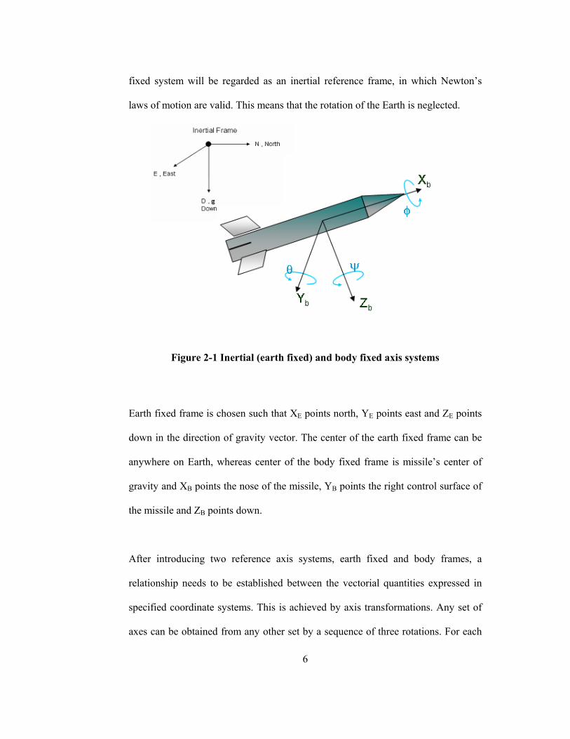
In this thesis two reference frames are used in the derivation as given in Figure 2-1;
Earth fixed axis system as inertial frame and body fixed axis system. The earth
6
fixed system will be regarded as an inertial reference frame, in which Newton’s
laws of motion are valid. This means that the rotation of the Earth is neglected.
Figure 2-1 Inertial (earth fixed) and body fixed axis systems
Earth fixed frame is chosen such that XE points north, YE points east and ZE points
down in the direction of gravity vector. The center of the earth fixed frame can be
anywhere on Earth, whereas center of the body fixed frame is missile’s center of
gravity and XB points the nose of the missile, YB points the right control surface of
the missile and ZB points down.
After introducing two reference axis systems, earth fixed and body frames, a
relationship needs to be established between the vectorial quantities expressed in
specified coordinate systems. This is achieved by axis transformations. Any set of
axes can be obtained from any other set by a sequence of three rotations. For each
7
rotation a transformation matrix is applied to the vectorial quantities. The final
transformation matrix is simply the product of the three matrices, multiplied in the
order of the rotations. The sequence of rotation is customarily taken as follows:
Rotate earth axes through some azimuthal angle Ψ about the axes ZE, to
obtain intermediate axes X1, Y1 and Z1.
Next rotate these axis X1, Y1 and Z1 through some angle of elevation Θ,
about the axes Y1, to obtain a second intermediate set of axes X2, Y2 and Z2.
Finally, rotate the new axes X2, Y2 and Z2 through an angle of bank Φ about
the axis, X2, to reach the body axes XB, YB and ZB.
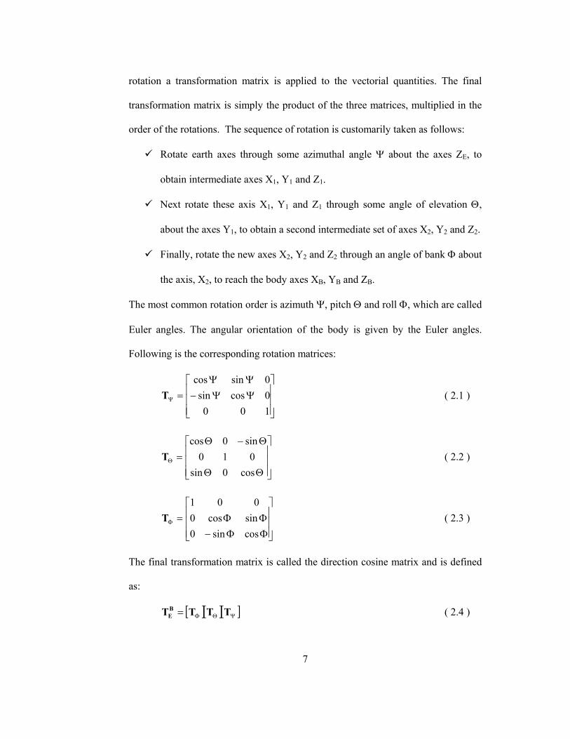
The most common rotation order is azimuth Ψ, pitch Θ and roll Φ, which are called
Euler angles. The angular orientation of the body is given by the Euler angles.
Following is the corresponding rotation matrices:
⎥⎥⎥
⎦
⎤
⎢⎢⎢
⎣
⎡ΨΨ−ΨΨ
=Ψ
1000cossin0sincos
T ( 2.1 )
⎥⎥⎥
⎦
⎤
⎢⎢⎢
⎣
⎡
ΘΘ
Θ−Θ=Θ
cos0sin010
sin0cosT ( 2.2 )
⎥⎥⎥
⎦
⎤
⎢⎢⎢
⎣
⎡
ΦΦ−ΦΦ=Φ
cossin0sincos0
001T ( 2.3 )
The final transformation matrix is called the direction cosine matrix and is defined
as:
[ ][ ][ ]ΨΘΦ= TTTTBE ( 2.4 )
8
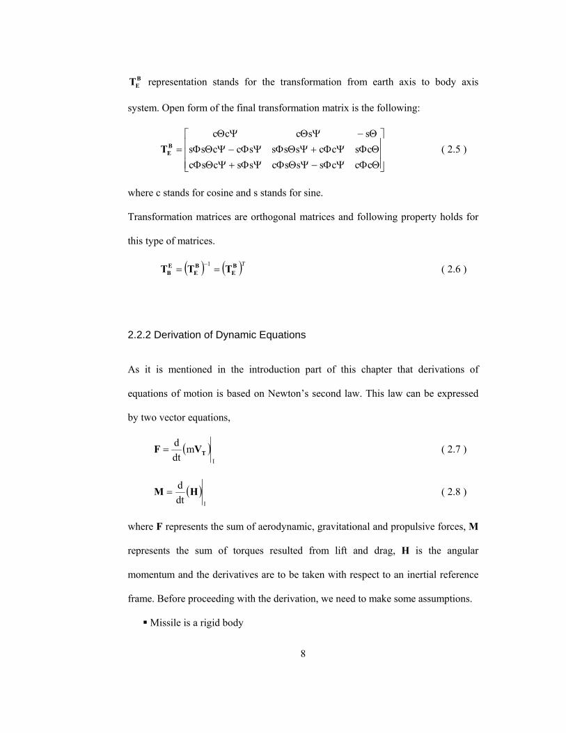
BET representation stands for the transformation from earth axis to body axis
system. Open form of the final transformation matrix is the following:
⎥⎥⎥
⎦
⎤
⎢⎢⎢
⎣
⎡
ΘΦΨΦ−ΨΘΦΨΦ+ΨΘΦΘΦΨΦ+ΨΘΦΨΦ−ΨΘΦΘ−ΨΘΨΘ
=cccssscsscsccsccssssccssssccc
BET ( 2.5 )
where c stands for cosine and s stands for sine.
Transformation matrices are orthogonal matrices and following property holds for
this type of matrices.
( ) ( )TBE
BE
EB TTT ==
−1 ( 2.6 )
2.2.2 Derivation of Dynamic Equations
As it is mentioned in the introduction part of this chapter that derivations of
equations of motion is based on Newton’s second law. This law can be expressed
by two vector equations,
( )I
mdtd
TVF = ( 2.7 )
( )Idt
d HM = ( 2.8 )
where F represents the sum of aerodynamic, gravitational and propulsive forces, M
represents the sum of torques resulted from lift and drag, H is the angular
momentum and the derivatives are to be taken with respect to an inertial reference
frame. Before proceeding with the derivation, we need to make some assumptions.
Missile is a rigid body

9
Mass of the missile remains constant
Considering these assumptions, Equation ( 2.7 ) and ( 2.8 ) can be re-expressed as,
( )Idt
dm TVF = ( 2.9 )
( )Idt
d HM = ( 2.10 )
Derivation of the equations for translational and rotational motions, which are the
results of force and moment equations respectively, will be dealt separately in the
following two sub-sections.
2.2.2.1 Translational Motion
Force equation given in ( 2.7 ) is written with respect to inertial frame (earth fixed
frame), so differentiation with respect to inertial frame while expressing the
vectorial quantities in body frame yields the following expression.
( ) ( ) ( ) ⎟⎟⎠
⎞⎜⎜⎝
⎛×+=≅ TTTT VωVVV
BEI dtd
dtd
dtd ( 2.11 )
where ω is the angular velocity of the missile with respect to the earth fixed axis
system. VT and ω can be expressed in body frame as follows,
wvu kjiVT ++= ( 2.12 )
rqp kjiω ++= ( 2.13 )
wvudtd
B
&&& kjiVT ++= ( 2.14 )
where i, j, and k are the unit vectors along XB, YB and ZB. Cross product term in
Equation 2.11 is given by,
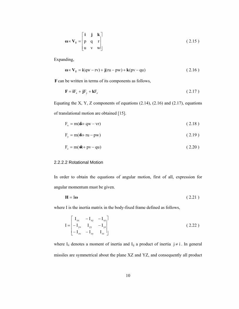
10
⎥⎥⎥
⎦
⎤
⎢⎢⎢
⎣
⎡=×
wvurqpkji
Vω T ( 2.15 )
Expanding,
)qupv()pwru()rvqw( −+−+−=× kjiVω T ( 2.16 )
F can be written in terms of its components as follows,
zyx FFF kjiF ++= ( 2.17 )
Equating the X, Y, Z components of equations (2.14), (2.16) and (2.17), equations
of translational motion are obtained [15].
)vrqwu(mFx −+= & ( 2.18 )
)pwruv(mFy −+= & ( 2.19 )
)qupvw(mFz −+= & ( 2.20 )
2.2.2.2 Rotational Motion
In order to obtain the equations of angular motion, first of all, expression for
angular momentum must be given.
ωH I= ( 2.21 )
where I is the inertia matrix in the body-fixed frame defined as follows,
⎥⎥⎥
⎦
⎤
⎢⎢⎢
⎣
⎡
−−−−−−
=
zzzyzx
yzyyyx
xzxyxx
IIIIIIIII
I ( 2.22 )
where Iii denotes a moment of inertia and Iij a product of inertia ij ≠ . In general
missiles are symmetrical about the plane XZ and YZ, and consequently all product
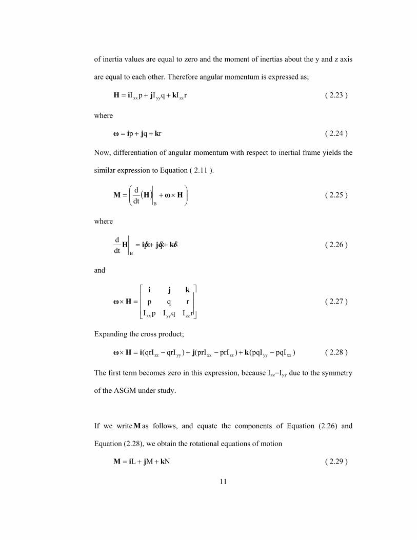
11
of inertia values are equal to zero and the moment of inertias about the y and z axis
are equal to each other. Therefore angular momentum is expressed as;
rIqIpI zzyyxx kjiH ++= ( 2.23 )
where
rqp kjiω ++= ( 2.24 )
Now, differentiation of angular momentum with respect to inertial frame yields the
similar expression to Equation ( 2.11 ).
( ) ⎟⎟⎠
⎞⎜⎜⎝
⎛×+= HωHM
Bdtd ( 2.25 )
where
rqpdtd
B
&&& kjiH ++= ( 2.26 )
and
⎥⎥⎥
⎦
⎤
⎢⎢⎢
⎣
⎡
=×rIqIpI
rqp
zzyyxx
kjiHω ( 2.27 )
Expanding the cross product;
)pqIpqI()prIprI()qrIqrI( xxyyzzxxyyzz −+−+−=× kjiHω ( 2.28 )
The first term becomes zero in this expression, because Izz=Iyy due to the symmetry
of the ASGM under study.
If we write M as follows, and equate the components of Equation (2.26) and
Equation (2.28), we obtain the rotational equations of motion
NML kjiM ++= ( 2.29 )
12
Rotational equations of motion are;
pIL xx &= ( 2.30 )
pr)II(qIM zzxxyy −+= & ( 2.31 )
pq)II(rIN xxyyzz −+= & ( 2.32 )
2.2.3 Derivation of Kinematic Equations
Position and attitude with respect to earth axis system is found using kinematic
equations.
2.2.3.1 Translational Kinematics
Velocity expressed in body axis system can be transformed to earth axis system by
the following expression
⎥⎥⎥
⎦
⎤
⎢⎢⎢
⎣
⎡=
⎥⎥⎥
⎦
⎤
⎢⎢⎢
⎣
⎡
wvu
zyx
EBT
&&&
( 2.33 )
where EBT is the transformation matrix from body axes system to earth axis system,
which is the transpose of BET (Equation ( 2.5 )), x, y and z are the location of the
body center of gravity, u, v and w are the velocity components along the body axes.
The open form of this equation is as follows:
( )( )ΨΦ+ΨΘΦ+
ΨΦ−ΨΘΦ+ΨΘ=sinsincossincosw
sincoscossinsinvcoscosux& ( 2.34 )
( )( )ΨΦ−ΨΘΦ+
ΨΦ+ΨΘΦ+ΨΘ=cossinsinsincosw
coscossinsinsinvsincosuy& ( 2.35 )
ΘΦ+ΘΦ+Θ−= coscoswcossinvsinuz& ( 2.36 )

13
2.2.3.2 Rotational Kinematics
It was stated that for transformation matrices, ( ) ( )TBE
BE
EB TTT ==
−1 , so from this,
following expression can be written.
( ) ITT =TB
EBE ( 2.37 )
Taking the derivative of this expression,
( ) ( ) 0TBE
BE
TBE
BE =+ TTTT && ( 2.38 )
( ) ( )( )TTBE
BE
TBE
BE TTTT && −= ( 2.39 )
The above equation indicates that ( )TBE
BE TT& is a skew symmetric matrix and so
there exists a skew symmetric matrix Ω generated from a column ω such that
( )TBE
BE TTΩ &= . ω is composed of the components of the angular velocity of the
body frame with respect to earth fixed frame expressed at the body frame.
Following is the expression for ω .
⎥⎥⎥
⎦
⎤
⎢⎢⎢
⎣
⎡=
rqp
ω ( 2.40 )
and the skew symmetric form of this vector is as follows,
⎥⎥⎥
⎦
⎤
⎢⎢⎢
⎣
⎡
−−
−=
0pqp0r
qr0Ω ( 2.41 )
Solving ( )TBE
BE TTΩ &= for the Euler angle rates, the rotational kinematic equations
are found as follows [15],
ΘΦ+Φ+=Ψ cos/)cosrsinq(p& ( 2.42 )

14
Φ−Φ=Θ sinrcosq& ( 2.43 )
ΘΦ+Φ+=Φ tan)cosrsinq(p& ( 2.44 )
This equation set has singularity when θ is equal to 90 (or 270) degrees. An
alternative method, which is called quaternions, is frequently used not to encounter
this singularity problem. For the munition considered here, 90 degrees pitch angle
is only attained when it hits the target, which is the end of the simulation. Therefore
quaternion equations are not required to be used for this munition.
2.3 Forces and Moments Acting on a Missile
Now we are in a position that if we know the forces and moments acting on the
munition, we can estimate the location of its center of gravity on earth, its velocity
and its heading. Therefore we need to define these forces and moments first, and
explain the ways to determine them.
There are mainly three types of forces acting on a rigid body missile; gravitational
force, aerodynamic force and thrust. The ASGM under study is a free falling
projectile without thrust, so we are left with gravitational and aerodynamic force.
Moments are the consequences of only aerodynamic forces, because gravity acts at
the center of gravity of the bomb, which is the center for body axes system.
2.3.1 Gravitational Force
The gravitational force acting on a missile is most obviously expressed in terms of
earth fixed frame. With respect to these axes the gravitational force is directed
15
along the ZE axis and its magnitude is assumed to be constant. Derived equations of
motion uses the body axes system, therefore gravitational force should be resolved
into body axes system by using transformation matrix from earth to body ( BET ).
⎥⎥⎥
⎦
⎤
⎢⎢⎢
⎣
⎡=
⎥⎥⎥
⎦
⎤
⎢⎢⎢
⎣
⎡
g00
Tggg
BE
z
y
x
( 2.45 )
Result of this multiplication is as follows;
⎥⎥⎥
⎦
⎤
⎢⎢⎢
⎣
⎡
ΦΘΦΘ
Θ−=
⎥⎥⎥
⎦
⎤
⎢⎢⎢
⎣
⎡
coscosgsincosg
sing
ggg
z
y
x
. ( 2.46 )
Gravitational forces represented in body frame are added to the force equations
obtained in Translational Motion section and the final form of these equations is as
follows,
)vrqwu(msinmgFAx −+=Θ− & ( 2.47 )
)pwruv(msincosgFAy −+=ΦΘ+ & ( 2.48 )
)qupvw(mcoscosgFAz −+=ΦΘ+ & ( 2.49 )
where FAx, FAy and FAz represent the aerodynamic forces.
2.3.2 Aerodynamic Forces and Moments
The aerodynamic forces and moments are represented by FAx, FAy, FAz and L, M, N
respectively. The most general expression for aerodynamic forces and moments are
as follows:
16
⎥⎥⎥
⎦
⎤
⎢⎢⎢
⎣
⎡=
⎥⎥⎥
⎦
⎤
⎢⎢⎢
⎣
⎡
z
y
x
d
Az
Ay
Ax
CCC
AQFFF
( 2.50 )
⎥⎥⎥
⎦
⎤
⎢⎢⎢
⎣
⎡=
⎥⎥⎥
⎦
⎤
⎢⎢⎢
⎣
⎡
n
m
l
d
CCC
AdQNML
( 2.51 )
where Qd is the dynamic pressure, A is the maximum cross-sectional area of the
bomb, d is the bomb diameter and Ci’s are the dimensionless aerodynamic force
and moment coefficients. The expression for dynamic pressure is as follows,
2Td V
21Q ρ= ( 2.52 )
where 222T WVUV ++=
In dynamic pressure expression ρ is the air density and it changes with altitude h,
which is down component of position vector with minus sign. Its change with
altitude is given below.
⎩⎨⎧
>×≤−ρ
=ρ−− 10000mh 10412.0
10000mh )h00002256.01())10000h(000151.0(
256.40 ( 2.53 )
where 0ρ is the air density at sea level (1.223 kg/m3). This formula is obtained by
curve fitting to the density variation in the ICAO standard atmosphere [15].
Dimensionless aerodynamic force and moment coefficients are designated as,
Cx : Axial force coefficient
Cy : Side force coefficient
Cz : Normal force coefficient
Cl : Rolling moment coefficient

17
Cm : Pitching moment coefficient
Cn : Yawing moment coefficient.
These aerodynamic force and moment coefficients are the functions of the Mach
number and flight parameters such as the angle of attack, side slip angle, the
control surface deflections ( are , , δδδ ), the body angular rates p, q, r. Subscripts e,
r and a stand for elevator, rudder and aileron deflections, respectively. So Ci can be
written as,
)r,q,p,,,,,,M(CC areii δδδβα= ( 2.54 )
Mach number is a dimensionless number defined as ratio of the total speed of the
body to the speed of sound estimated at the altitude of the body. The expression for
Mach number is given below.
CV
M T= ( 2.55 )
where C is the speed of sound and can be calculated as follows,
RTC γ= ( 2.56 )
In the speed of sound equation γ is the specific heat ratio of the air which is 1.4,
and R is the universal air gas constant which is equal to 287 J/kgK. T is the
ambient temperature which also changes with altitude and can be expressed as,
⎩⎨⎧
>×≤−
=10000mh 7744.0T10000mh )000002256.1(T
T0
0 ( 2.57 )
where T0 is the temperature at sea level and is equal to 293 K. This formula is
obtained by curve fitting to the temperature variation in the ICAO standard
atmosphere [15].
18
Angle of attack and side slip angle are defined by the following expressions. These
angles are important because they orient the lift and drag forces with respect to
body frame.
⎟⎠⎞
⎜⎝⎛=α
uwtana ( 2.58 )
⎟⎟⎠
⎞⎜⎜⎝
⎛=β
TVvsina ( 2.59 )
Angle of attack and side slip angle expressions can be further simplified due to the
fact that w and v being much smaller when compared with u. Moreover u can be
taken equal to VT, since v and w are much smaller than u. Simplified expressions
for angle of attack and side slip angle are given below.
uw
=α ( 2.60 )
uv
=β ( 2.61 )
As it is mentioned in the previous paragraphs, aerodynamic coefficients are
nonlinear functions of Mach number and flight parameters. If this relationship is
linearized using Taylor series expansion, following expression is obtained.
T.O.HV2dr)M(C
V2dq)M(C
V2dp)M(C)M(C)M(C
)M(C)M(C)M(C)M(CC
Tir
Tiq
Tipaairri
eeiii0ii
++
++δ+δ
+δ+β+α+=
δδ
δβα
( 2.62 )
where H.O.T stands for higher order terms. θiC and θ&iC are the short hand notations
for the derivative of aerodynamic coefficient with respect to θ and θ&, as given

19
below. θ and θ& stand for the angle quantities such as α, β etc., and angle rate
quantities, such as p, q and r, respectively.
θ∂∂
=θi
iC)M(C ( 2.63 )
⎟⎟⎠
⎞⎜⎜⎝
⎛θ∂
∂=θ
T
ii
V2d
C)M(C
&& ( 2.64 )
These aerodynamic coefficients can be estimated using wind tunnels, CFD
(Computational Fluid Dynamics) methods and softwares like Missile Datcom. In
this thesis Missile Datcom is used in the calculation of aerodynamic coefficients.
Missile Datcom is run for a number of Mach number values and the coefficients are
inserted in a look-up table as a function of Mach number, which calculates the
aerodynamic coefficients by interpolating the coefficients corresponding to nearby
Mach number values.
Expressions (2.63) and (2.64) are general expressions for aerodynamic force and
moment coefficients. Particular expressions for each aerodynamic force and
moment coefficients are given below.
)M(CC 0xx = ( 2.65 )
Tyrrryyy V2
dr)M(C)M(C)M(CC +δ+β= δβ ( 2.66 )
Tzqeezzz V2
dq)M(C)M(C)M(CC +δ⋅+α= δα ( 2.67 )
Tlpaall V2
dp)M(C)M(CC +δ= δ ( 2.68 )

20
Tmqeemmm V2
dq)M(C)M(C)M(CC +δ+α= δα ( 2.69 )
Tnrrrnnn V2
dr)M(C)M(C)M(CC +δ+β= δβ ( 2.70 )
Number of aerodynamic coefficients used in the simulations and controller design
can be reduced considering Maple-Synge rotational symmetry analysis on linear
transverse aerodynamic forces and moments for a missile which has a symmetry
with respect to its y and z axis. This analysis shows that, [15]
βα = yz CC
ryez CC δδ =
yrzq CC −=
βα −= nm CC
rnem CC δδ −=
nrmq CC =

21
CHAPTER 3
3 SYSTEM IDENTIFICATION FOR THE CONTROL
ACTUATION SYSTEM
3.1 Introduction
System identification deals with the problem of building mathematical models of
dynamical systems based on observed data from the systems. In other words, the
problem of system identification is the determination of the system model from
records of input u(t) and output y(t). There are different types of system
identification analysis which can be used depending on the application. Frequency
response identification, impulse response identification by deconvolution and
identification from correlation functions are the examples of the ones that do not
result in transfer function. There are also other approaches that find the coefficients
of the assumed parametric transfer functions, such as least squares, maximum
likelihood (Prediction Error Method). In this thesis we used the MATLAB System
Identification Toolbox in order to solve system identification problem.
Input of the CAS is the voltages applied to the solenoid valves. Solenoid valves are
either closed or open according to the voltages applied which are either 24 V or

22
ground. Output of the control actuation system is the resulted shaft angle. Input and
output data pairs are collected by the PC with data acquisition cards. Cards are
chosen to be compatible with MATLAB Real Time Windows Target toolbox. Shaft
angles are measured by two transducers, absolute encoder and arc segment
potentiometer.
This chapter starts with the description of the Control Actuation System of this
munition. Because MATLAB System Identification Toolbox is used in system
identification studies, a brief introduction to this toolbox is given next. At the end,
various CAS models, estimated using this toolbox, are given together with their
fitness values to the validation data set.
3.2 Control Actuation System Setup
3.2.1 Description of Control Actuation System
Control actuation system in a missile realizes the autopilot commands in order to
steer the missile to the target. There are mainly three types of control actuation
system: Electro-hydraulic, electromechanical and electro-pneumatic. All of them
find use in missiles according to their mission. For example hydraulic actuators are
mostly used in long-range ballistic missiles such as Patriot, Pershing I and II, where
high power is required to maneuver the missile and large space is available for
huge hydraulic CAS. Missiles such as stinger having small control surfaces use
electromechanical actuators usually. Pneumatic actuators are used in missiles
which require high power, explosion-proof character and easy maintenance.

23
Copperhead and Tomahawk are the examples of such systems having pneumatic
actuators. The difference between the hydraulic and pneumatic actuators is in the
type of the fluids that they make use of to transmit power. Pneumatic actuators use
gas, such as air or nitrogen gas, whereas hydraulic actuators use liquids, mostly oil.
The missile under consideration is a type of ASGM (Air to Surface Guided
Munition) and it uses pneumatic CAS. The fluid it uses is nitrogen. Due to the
bang-trial-bang nature of the missile, pneumatic CAS was also designed in bang-
trial-bang nature. In other words, canards drived by CAS are in either 10 degrees
deflection, or -10 degrees deflection. The trial case corresponds to the situation in
which no guidance commands are generated. In that case canards are aligned with
the streamline.
CAS under consideration is composed of following components;
Nitrogen bottle: Pressure vessel where the pressurized (55 MPa) nitrogen gas
is kept.
Regulator: It regulates the pressure of the nitrogen coming from the pressure
vessel to 6.5 to 9 Mpa.
Dampers: There are two dampers in the system. They are used in damping
aerodynamic forces on the canards. They are both viscous and spring dampers.
Solenoid valves: There are two five-way solenoid valves in the system, which
are controlling the motion in pitch and yaw planes. Each solenoid valve can be
thought of union of two three-way solenoid valves, which can be energized
independent of each other. One is responsible for the positive deflection of the
canard, the other one is responsible for the negative deflection. After this point
24
we will call them as pos-solenoid valve and neg-solenoid valve. The main
function of solenoid valve is to let the gas go to one of the cylinders and empty
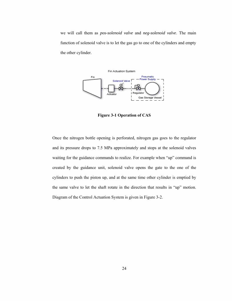
the other cylinder.
Figure 3-1 Operation of CAS
Once the nitrogen bottle opening is perforated, nitrogen gas goes to the regulator
and its pressure drops to 7.5 MPa approximately and stops at the solenoid valves
waiting for the guidance commands to realize. For example when “up” command is
created by the guidance unit, solenoid valve opens the gate to the one of the
cylinders to push the piston up, and at the same time other cylinder is emptied by
the same valve to let the shaft rotate in the direction that results in “up” motion.
Diagram of the Control Actuation System is given in Figure 3-2.
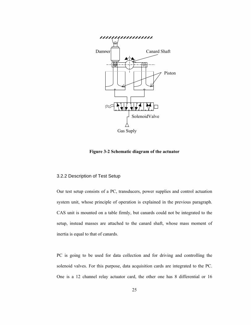
25
Figure 3-2 Schematic diagram of the actuator
3.2.2 Description of Test Setup
Our test setup consists of a PC, transducers, power supplies and control actuation
system unit, whose principle of operation is explained in the previous paragraph.
CAS unit is mounted on a table firmly, but canards could not be integrated to the
setup, instead masses are attached to the canard shaft, whose mass moment of
inertia is equal to that of canards.
PC is going to be used for data collection and for driving and controlling the
solenoid valves. For this purpose, data acquisition cards are integrated to the PC.
One is a 12 channel relay actuator card, the other one has 8 differential or 16
Gas Suply
SolenoidValve
Damper Canard Shaft
Piston

26
single-ended analog input channels, 2 analog output channels and 24 channel
digital I/O.
There are two different angle measurement devices in the test setup; one is an arc
segment potentiometer, the other one is a Heidenhein absolute encoder with model
number ROC 417. Arc segment potentiometer is especially used in fin or wing
actuators, because the maximum angle that fin can rotate is limited to some angle,
therefore a potentiometer that can measure a full rotation is not required for these
types of applications, indeed arc segment potentiometer is preferred in order to
save space. Encoder is both incremental and absolute encoder. Its incremental
measurement has the resolution of 8192 lines. Absolute output of the encoder is a
digital signal in EnDAT format with 17 bit resolution. An electronic card is
designed to be able to read the digital output of the encoder, which is required to
convert from EnDAT data format to parallel digital data. Specifications of these
measurement devices are given in APPENDIX B.
A block schema showing the connection of these measurement devices and data
acquisition cards is given in Figure 3-3. Energizing voltage for the solenoid valves
are switched by the relays and relays are controlled by the PC. Analog
potentiometer signal is recorded by the 16 bit A/D board and digital encoder
signals are recorded by the 24 Channel Digital I/O board. There seems no problem
in recording the resulted canard shaft rotation by potentiometer and encoder, but
input signal level, which is 24 V, is too high to be collected by 16 bit A/D board.
Therefore another input signal with 1 Volt level is switched by the relay card. This
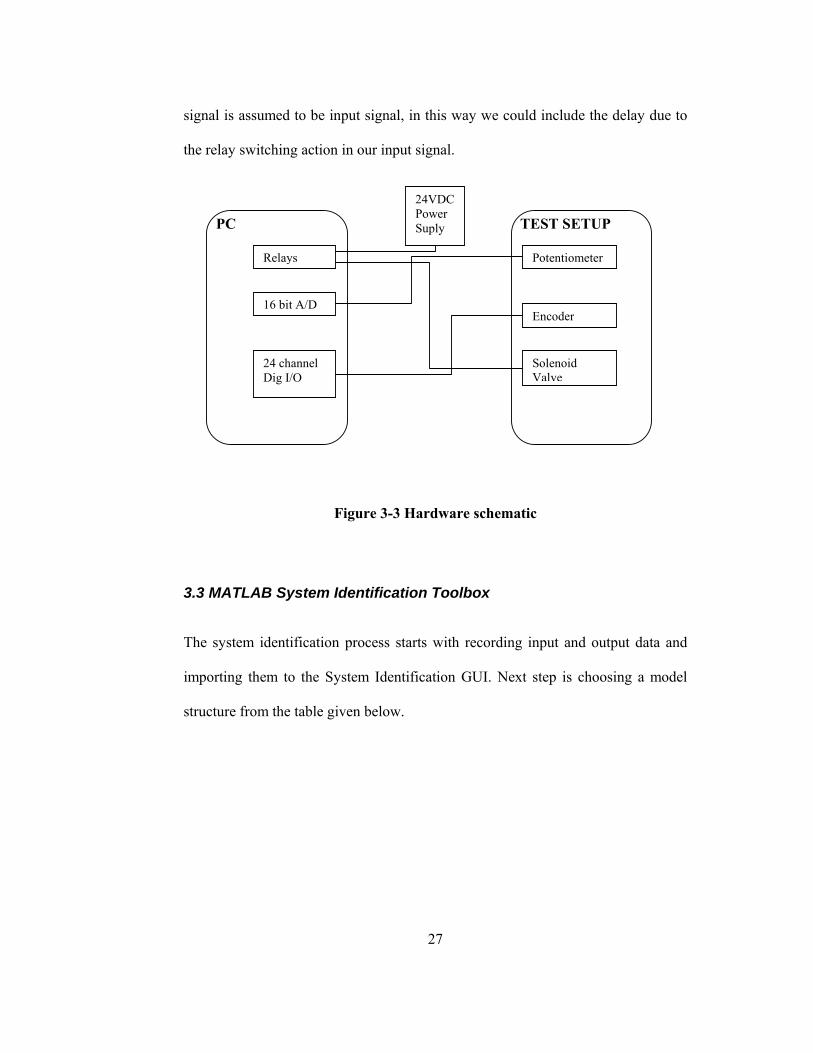
27
signal is assumed to be input signal, in this way we could include the delay due to
the relay switching action in our input signal.
Figure 3-3 Hardware schematic
3.3 MATLAB System Identification Toolbox
The system identification process starts with recording input and output data and
importing them to the System Identification GUI. Next step is choosing a model
structure from the table given below.
24VDC Power Suply PC TEST SETUP
Potentiometer
Encoder
Solenoid Valve
Relays
16 bit A/D
24 channel Dig I/O
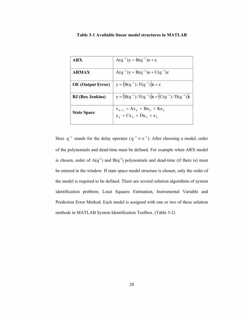
28
Table 3-1 Available linear model structures in MATLAB
ARX eu)q(By)q(A 11 += −−
ARMAX e)q(Cu)q(By)q(A 111 −−− +=
OE (Output Error) ( ) eu)q(F/)q(By 11 += −−
BJ (Box Jenkins) ( ) ( )e)q(D/)q(Cu)q(F/)q(By 1111 −−−− +=
State Space kkkk
kkk1k
eDuCxyKeBuAxx
++=++=+
Here 1q − stands for the delay operator ( 11 zq −− ≡ ). After choosing a model, order
of the polynomials and dead-time must be defined. For example when ARX model
is chosen, order of A(q-1) and B(q-1) polynomials and dead-time (if there is) must
be entered in the window. If state space model structure is chosen, only the order of
the model is required to be defined. There are several solution algorithms of system
identification problem; Least Squares Estimation, Instrumental Variable and
Prediction Error Method. Each model is assigned with one or two of these solution
methods in MATLAB System Identification Toolbox. (Table 3-2)
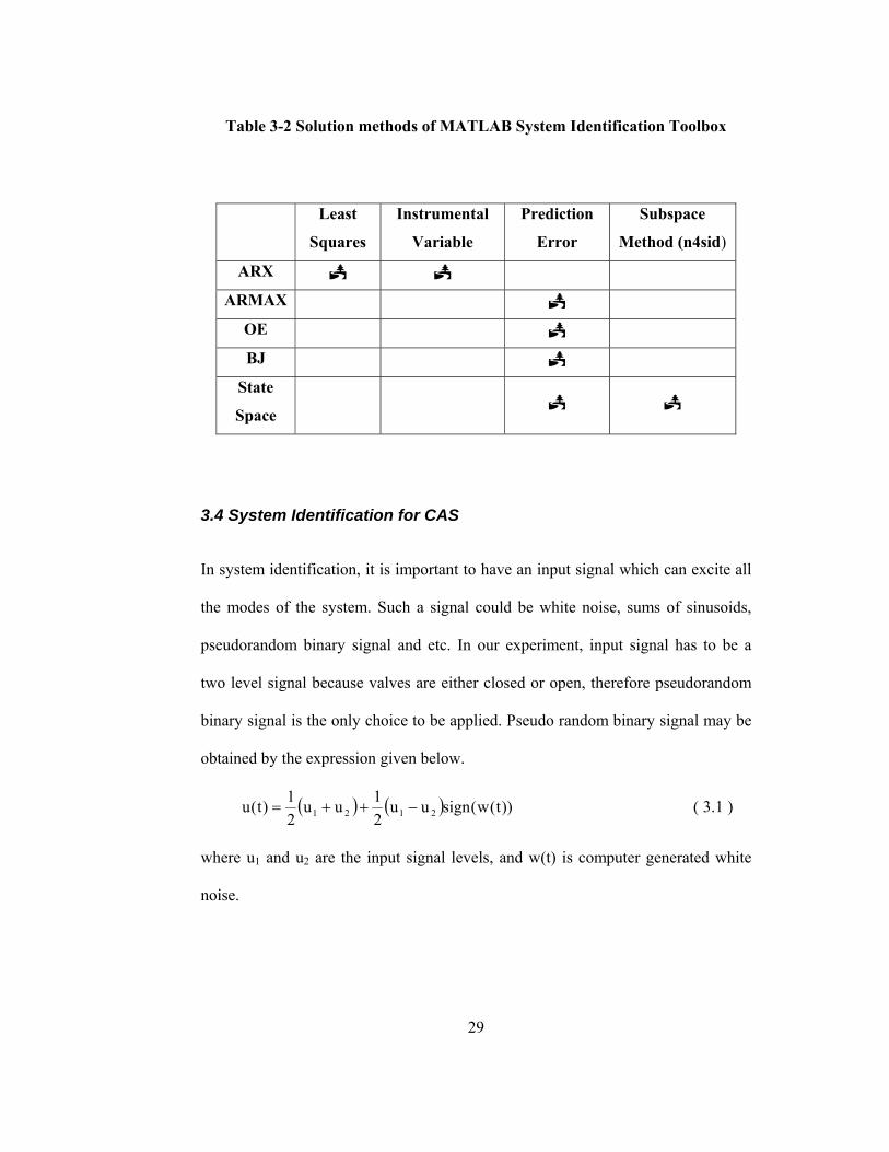
29
Table 3-2 Solution methods of MATLAB System Identification Toolbox
Least
Squares
Instrumental
Variable
Prediction
Error
Subspace
Method (n4sid)
ARX
ARMAX
OE
BJ
State
Space
3.4 System Identification for CAS
In system identification, it is important to have an input signal which can excite all
the modes of the system. Such a signal could be white noise, sums of sinusoids,
pseudorandom binary signal and etc. In our experiment, input signal has to be a
two level signal because valves are either closed or open, therefore pseudorandom
binary signal is the only choice to be applied. Pseudo random binary signal may be
obtained by the expression given below.
( ) ( ) ))t(w(signuu21uu
21)t(u 2121 −++= ( 3.1 )
where u1 and u2 are the input signal levels, and w(t) is computer generated white
noise.
30
System identification studies are carried out using two different schemes. In the
first one, pseudo random binary signal is generated in the PC, whose level is
between 0 and 1 (means relay open and relay close), and this signal applied to the
neg-solenoid valve and pos-solenoid valve separately. For example in the neg-
solenoid valve using case, canard shaft moves between 0 degrees and
approximately -10 degrees and in the pos-solenoid valve case, it moves between 0
degrees and approximately 10 degrees.
In the second one, the level of the binary signal changes from -1 to 1. Here -1
means energizing the neg-solenoid valve, while the pos-solenoid valve is in normal
position and +1 means energizing the pos-solenoid valve, while the neg-solenoid
valve is brought to normal position. With this scheme, canard shaft deflection
changes from approximately -10 degrees to +10 degrees. These two schemes will
make two different pulse width modulation schemes possible, which are explained
in the fourth chapter.
3.4.1 System Identification Using First Scheme
Input-output data is collected with sampling frequency 1 kHz for both negative and
positive shaft rotations for 2 minutes. The first 1 minute duration data is used for
identification, the last 1 minute data is used for validation. First 45 second of this
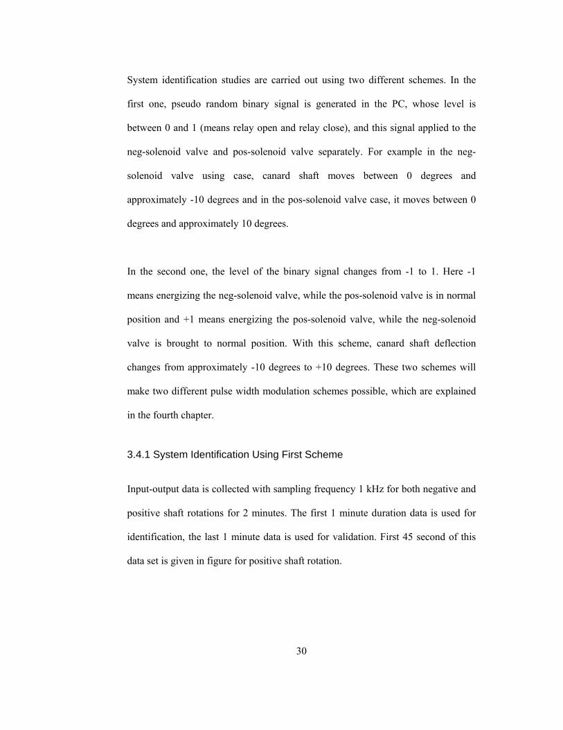
data set is given in figure for positive shaft rotation.
31
Figure 3-4 Some portion of input-output data set for positive deflection
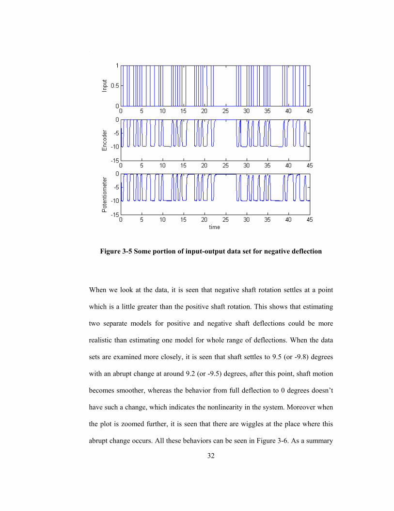
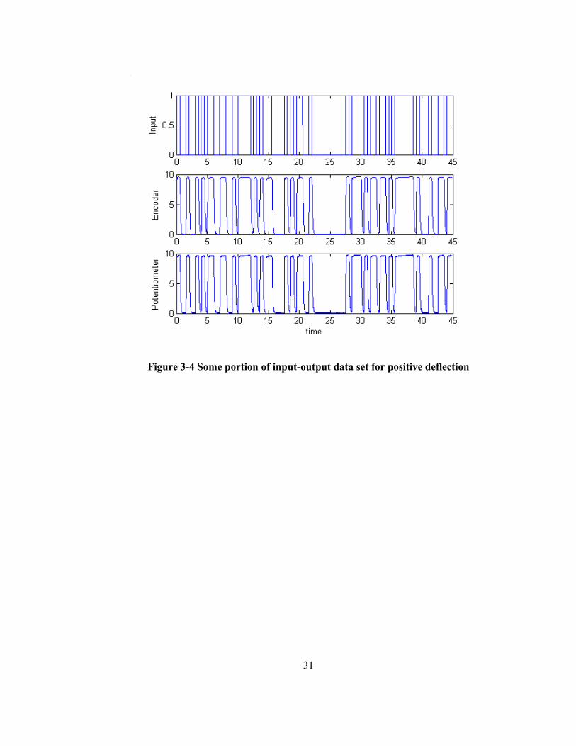
32
Figure 3-5 Some portion of input-output data set for negative deflection
When we look at the data, it is seen that negative shaft rotation settles at a point
which is a little greater than the positive shaft rotation. This shows that estimating
two separate models for positive and negative shaft deflections could be more
realistic than estimating one model for whole range of deflections. When the data
sets are examined more closely, it is seen that shaft settles to 9.5 (or -9.8) degrees
with an abrupt change at around 9.2 (or -9.5) degrees, after this point, shaft motion
becomes smoother, whereas the behavior from full deflection to 0 degrees doesn’t
have such a change, which indicates the nonlinearity in the system. Moreover when
the plot is zoomed further, it is seen that there are wiggles at the place where this
abrupt change occurs. All these behaviors can be seen in Figure 3-6. As a summary

33
if we interpret this motion, it seems that at the beginning the effect of damper on
the shaft motion is quite less, but after some deflection angle, it damps the motion
very quickly. Although it seems very difficult to fit a linear model to these data sets
showing this much of non-linearity, this is the only choice unless a parametric
nonlinear dynamic model is built.
Figure 3-6 Zoomed view of the output data
The order of the model structure can be at most 4, because moving mass (plunger)
in the solenoid valve and rotating shaft can be modeled as second order systems.
However we have no idea about the number of zeros and delays. In order to decide
34
on which model is any good, the fitness of the estimated model simulations to the
validation data must be considered. In the light of this information, many models
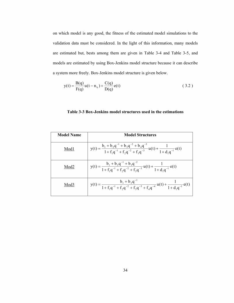
are estimated but, bests among them are given in Table 3-4 and Table 3-5, and
models are estimated by using Box-Jenkins model structure because it can describe
a system more freely. Box-Jenkins model structure is given below.
)t(e)q(D)q(C)nt(u
)q(F)q(B)t(y k +−= ( 3.2 )
Table 3-3 Box-Jenkins model structures used in the estimations
Model Name Model Structures
Mod1 )t(eqd1
1)t(uqfqfqf1
qbqbqbb)t(y 1
13
32
21
1
34
23
121
−−−−
−−−
++
++++++
=
Mod2 )t(eqd1
1)t(uqfqfqf1
qbqbb)t(y 1
13
32
21
1
23
121
−−−−
−−
++
+++++
=
Mod3 )t(eqd1
1)t(uqfqfqfqf1
qbb)t(y 1
14
43
32
21
1
121
−−−−−
−
++
+++++
=

35
Table 3-4 Estimated model transfer functions from positive shaft rotation data
set
Pot. Data )2762s59.39s)(53.11s(
)10596.3s06.97s)(4292s(0019509.02
42
+++⋅+++
Mod1 Encoder
Data )4263s24.45s)(38.13s(
)10619.5s122s)(2309s(004183.02
42
+++⋅+−+
Pot. Data )3023s08.40s)(71.11s(
)1021.4s78.12s)(1045s(0076361.02
42
+++⋅+−+
Mod2 Encoder
Data )4176s64.45s)(71.12s(
)10987.4s3.139s)(1106s(0076361.02
42
+++⋅+−+
Pot. Data )2877s54.40s)(913.5s)(62.11s(
)10491.8s5.809s)(913.5s)(7.727s(00051537.02
52
++++⋅++++
Mod3 Encoder
Data )3778s31.47s)(96.12s)(28.29s(
)1018.1s1006s)(18.25s)(4.875s(00052444.02
62
++++⋅++++

36
Table 3-5 Estimated model transfer functions from negative shaft rotation
data set
Pot. Data )2377s12.38s)(51.12s(
)10199.1s074.9s)(10053.1s(0022485.02
424
+++⋅++⋅+−
Mod1 Encoder
Data )2.529s47.41s)(5898.0s(
)10837.4s9.230s)(5898.0s(010159.02
52
+++⋅+++−
Pot. Data )6.554s86.42s)(248.2s(
)249.2s)(482s)(1069s(0098938.02 +++
+−+
Mod2 Encoder
Data )3212s36.51s)(08.14s(
)10247.3s41.48s)(1065s(01282.02
42
+++⋅+−+−
Pot. Data )1956s1.39s)(1.12s)(42.74s(
)10917.4s6.921s)(46.74s)(2.209s(0021936.02
52
++++⋅++++−
Mod3 Encoder
Data )1751s02.37s)(88.13s)(39.25s(
)10858.4s2.942s)(4.25s)(6.154s(0031143.02
52
++++⋅++++−
Models estimated by MATLAB System Identification Toolbox are all discrete time
but we preferred to interpret the results in continuous time. Therefore, before
tabulating the results, estimated models are converted to continuous time with d2c
MATLAB function. In other words, continuous time models are only used to be
presented in these tables, and in controller design process for example, discrete
time models are used.
37
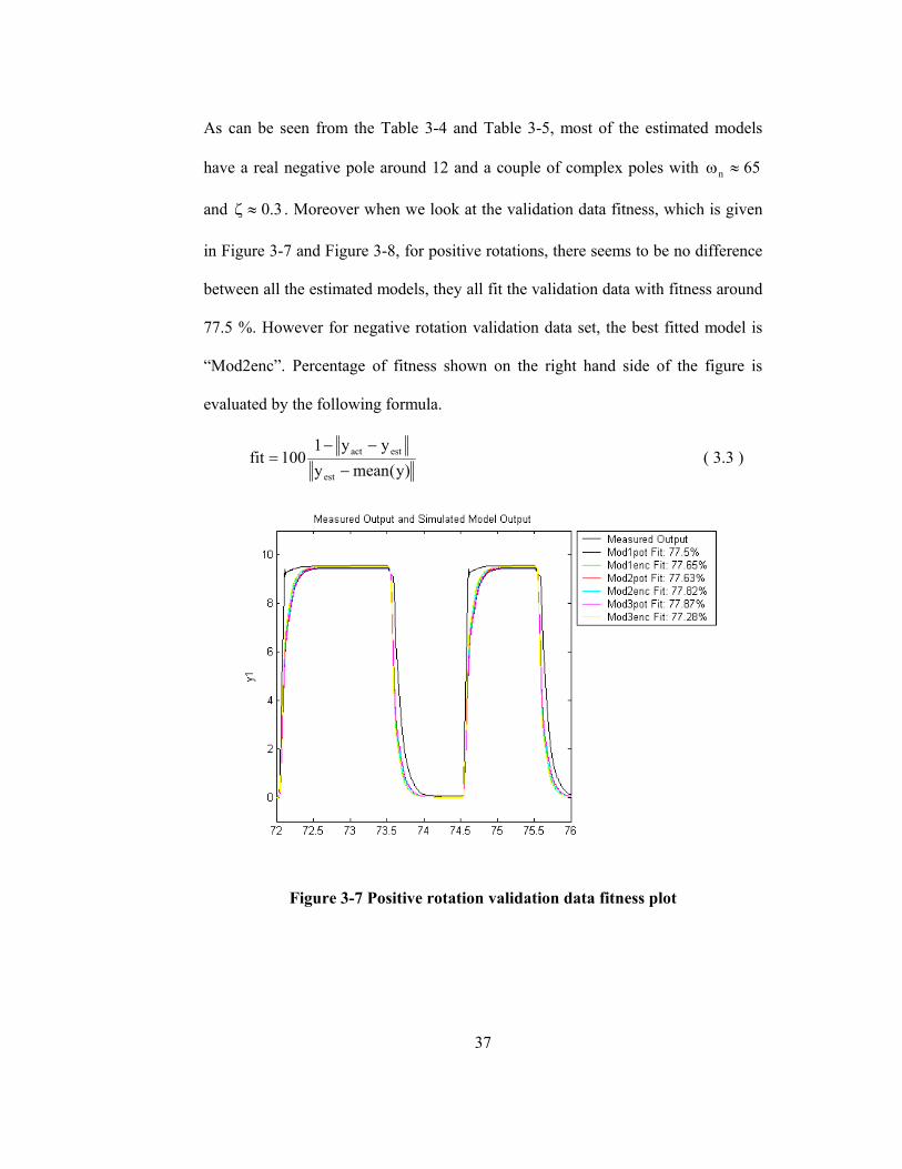
As can be seen from the Table 3-4 and Table 3-5, most of the estimated models
have a real negative pole around 12 and a couple of complex poles with 65n ≈ω
and 3.0≈ζ . Moreover when we look at the validation data fitness, which is given
in Figure 3-7 and Figure 3-8, for positive rotations, there seems to be no difference
between all the estimated models, they all fit the validation data with fitness around
77.5 %. However for negative rotation validation data set, the best fitted model is
“Mod2enc”. Percentage of fitness shown on the right hand side of the figure is
evaluated by the following formula.
)y(meany
yy1100fit
est
estact
−
−−= ( 3.3 )
Figure 3-7 Positive rotation validation data fitness plot

38
Figure 3-8 Negative rotation validation data fitness plot
As a result for positive and negative rotation models, “Mod2enc” models are
chosen, whose continuous and discrete time transfer functions are given below.
For positive rotations:
)4176s64.45s)(71.12s()10987.4s3.139s)(1106s(0076361.0)s(G 2
42
pos +++⋅+−+
= ( 3.4 )
)9554.0z951.1z)(9874.0z()155.1z101.2z(z0091481.0)z(G 2
2
pos +−−+−
= ( 3.5 )
For negative rotations:
)3212s36.51s)(08.14s()10247.3s41.48s)(1065s(01282.0)s(G 2
42
neg +++⋅+−+−
= ( 3.6 )
)9499.0z947.1z)(986.0z()052.1z018.2z(z01282.0)z(G 2
2
neg +−−+−−
= ( 3.7 )

39
3.4.2 System Identification Using Second Scheme
Input-output data is collected with sampling frequency 1 kHz for 2 minutes. The
first 1 minute duration data is used for identification, the last 1 minute data is used
for validation. First 45 second of this data set is given in figure below.
Figure 3-9 Some portion of input-output data set
For this data set, there is no difference in the settling characteristic in positive full
deflection angle and the settling characteristic in negative full deflection angle,
which was not the case in the first scheme. Therefore it is expected to better fit a
model using this data set. Again Box-Jenkins model structures given in Table 3-6
are used in the model structures.
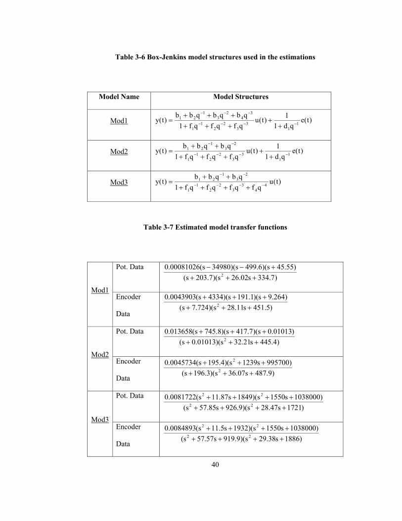
40
Table 3-6 Box-Jenkins model structures used in the estimations
Model Name Model Structures
Mod1 )t(eqd1
1)t(uqfqfqf1
qbqbqbb)t(y 1
13
32
21
1
34
23
121
−−−−
−−−
++
++++++
=
Mod2 )t(eqd1
1)t(uqfqfqf1
qbqbb)t(y 1
13
32
21
1
23
121
−−−−
−−
++
+++++
=
Mod3 )t(uqfqfqfqf1
qbqbb)t(y 4
43
32
21
1
23
121
−−−−
−−
++++++
=
Table 3-7 Estimated model transfer functions
Pot. Data )7.334s02.26s)(7.203s(
)55.45s)(6.499s)(34980s(00081026.02 +++
+−−
Mod1 Encoder
Data )5.451s11.28s)(724.7s(
)264.9s)(1.191s)(4334s(0043903.02 +++
+++
Pot. Data )4.445s21.32s)(01013.0s(
)01013.0s)(7.417s)(8.745s(013658.02 +++
+++
Mod2 Encoder
Data )9.487s07.36s)(3.196s(
)995700s1239s)(4.195s(0045734.02
2
++++++
Pot. Data )1721s47.28s)(9.926s85.57s(
)1038000s1550s)(1849s87.11s(0081722.022
22
++++++++
Mod3 Encoder
Data )1886s38.29s)(9.919s57.57s(
)1038000s1550s)(1932s5.11s(0084893.022
22
++++++++

41
The estimated models are given in Table 3-7. From the table it can be said that,
estimated models from potentiometer data are not identical with the estimated
models from encoder except for “Mod3”. This model has a fourth order dynamics
and it also fits the validation data best, which is given below in Figure 3-10.
Therefore this model is chosen and its continuous-time and discrete-time transfer
functions are given in Equation (3.8) and (3.9).
Figure 3-10 Validation data fitness plot
)1886s38.29s)(9.919s57.57s()10038.1s1550s)(1932s5.11s(0084893.0)s(G 22
622
++++⋅++++
= ( 3.8 )
)971.0z969.1z)(9441.0z943.1z()9886.0z987.1z(z0084893.0)z(G 22
22
+−+−+−
= ( 3.9 )

42
CHAPTER 4
4 CONTROLLER DESIGN WITH PWM FOR CONTROL
ACTUATION SYSTEM
4.1 Introduction
After we estimate control actuation system models, a controller is required to be
designed. But although the mathematical model of CAS can take values different
from 1, it is known that physically it doesn’t take such values. Therefore controller
output should be composed of two values, which corresponds to energized solenoid
valve and normal solenoid valve situations. The most famous solution for this type
of situations is “Pulse Width Modulation”, which means adjusting the width of the
“energize the solenoid valve” signal according to the magnitude of the controller
signal.
This chapter starts with the definition of PWM and continues with description of
controller and simulation results of the closed loop control actuation system.
43
4.2 Pulse Width Modulation
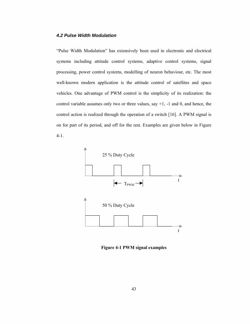
“Pulse Width Modulation” has extensively been used in electronic and electrical
systems including attitude control systems, adaptive control systems, signal
processing, power control systems, modelling of neuron behaviour, etc. The most
well-known modern application is the attitude control of satellites and space
vehicles. One advantage of PWM control is the simplicity of its realization: the
control variable assumes only two or three values, say +1, -1 and 0, and hence, the
control action is realized through the operation of a switch [16]. A PWM signal is
on for part of its period, and off for the rest. Examples are given below in Figure
4-1.
Figure 4-1 PWM signal examples
TPWM t
25 % Duty Cycle
t
50 % Duty Cycle
44
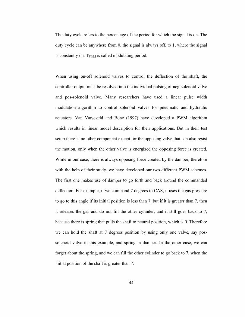
The duty cycle refers to the percentage of the period for which the signal is on. The
duty cycle can be anywhere from 0, the signal is always off, to 1, where the signal
is constantly on. TPWM is called modulating period.
When using on-off solenoid valves to control the deflection of the shaft, the
controller output must be resolved into the individual pulsing of neg-solenoid valve
and pos-solenoid valve. Many researchers have used a linear pulse width
modulation algorithm to control solenoid valves for pneumatic and hydraulic
actuators. Van Varseveld and Bone (1997) have developed a PWM algorithm
which results in linear model description for their applications. But in their test
setup there is no other component except for the opposing valve that can also resist
the motion, only when the other valve is energized the opposing force is created.
While in our case, there is always opposing force created by the damper, therefore
with the help of their study, we have developed our two different PWM schemes.
The first one makes use of damper to go forth and back around the commanded
deflection. For example, if we command 7 degrees to CAS, it uses the gas pressure
to go to this angle if its initial position is less than 7, but if it is greater than 7, then
it releases the gas and do not fill the other cylinder, and it still goes back to 7,
because there is spring that pulls the shaft to neutral position, which is 0. Therefore
we can hold the shaft at 7 degrees position by using only one valve, say pos-
solenoid valve in this example, and spring in damper. In the other case, we can
forget about the spring, and we can fill the other cylinder to go back to 7, when the
initial position of the shaft is greater than 7.
45
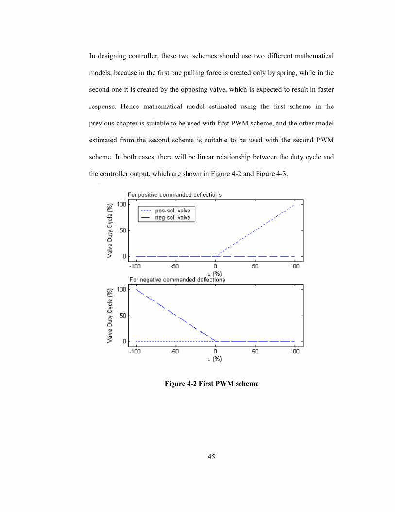
In designing controller, these two schemes should use two different mathematical
models, because in the first one pulling force is created only by spring, while in the
second one it is created by the opposing valve, which is expected to result in faster
response. Hence mathematical model estimated using the first scheme in the
previous chapter is suitable to be used with first PWM scheme, and the other model
estimated from the second scheme is suitable to be used with the second PWM
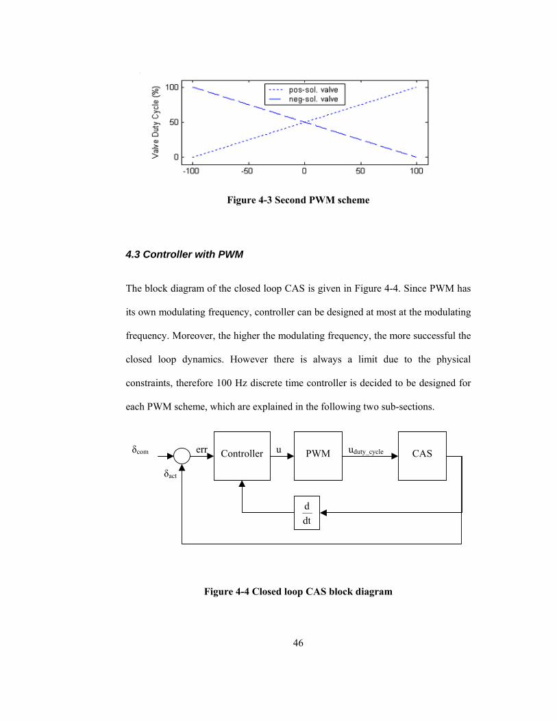
scheme. In both cases, there will be linear relationship between the duty cycle and
the controller output, which are shown in Figure 4-2 and Figure 4-3.
Figure 4-2 First PWM scheme
46
Figure 4-3 Second PWM scheme
4.3 Controller with PWM
The block diagram of the closed loop CAS is given in Figure 4-4. Since PWM has
its own modulating frequency, controller can be designed at most at the modulating
frequency. Moreover, the higher the modulating frequency, the more successful the
closed loop dynamics. However there is always a limit due to the physical
constraints, therefore 100 Hz discrete time controller is decided to be designed for
each PWM scheme, which are explained in the following two sub-sections.
Figure 4-4 Closed loop CAS block diagram
CAS
Controller
PWM δcom err u uduty_cycle
δact
dtd

47
4.3.1 Controller for First PWM Scheme
Controller structure is chosen to be PI with rate feedback, since taking derivative
from a digital position sensor can be said to be noiseless. As it is mentioned before
in this scheme, mathematical model of CAS is the one that is given in Section
3.4.1. For convenience, its discrete-time mathematical model is repeated below.
For positive rotations
)9554.0z951.1z)(9874.0z()155.1z101.2z(z0091481.0)z(G 2
2
pos +−−+−
= ( 4.1 )
For negative rotations
)9499.0z947.1z)(986.0z()052.1z018.2z(z01282.0)z(G 2
2
neg +−−+−−
= ( 4.2 )
As can be seen from the transfer functions, the magnitude of the poles, the zeros
and the gains are very close to each other. The sign of them are also the same in
two transfer functions, except for gains. Therefore reducing these transfer functions
into single transfer function for controller design purposes will not create a
problem, as long as we show that controller, which is designed for the single
transfer function, works well with these two transfer functions.
Reducing the model into single transfer function is made by averaging the poles,
zeros and absolute value of the gains. Single transfer function is given below
)9526.0z949.1z)(9867.0z()102.1z06.2z(z010984.0)z(G 2
2
mean +−−+−
= ( 4.3 )

48
Controller for this single transfer function is designed by trail and error process.
Figure 4-5 shows the closed loop model built in MATLAB Simulink and Figure
4-6 shows inside of the designed controller.
Figure 4-5 Closed loop CAS model built in MATLAB
Figure 4-6 Inside of MATLAB controller block for first PWM scheme
49
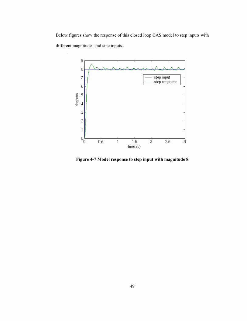
Below figures show the response of this closed loop CAS model to step inputs with
different magnitudes and sine inputs.
Figure 4-7 Model response to step input with magnitude 8
50
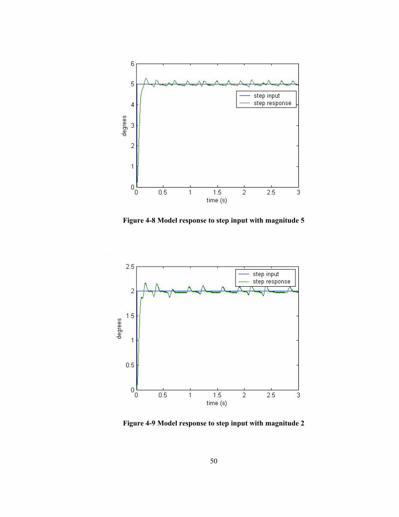
Figure 4-8 Model response to step input with magnitude 5
Figure 4-9 Model response to step input with magnitude 2

51
Figure 4-10 Response of the model to the sine input with amplitude 8 and
frequency 1 Hz
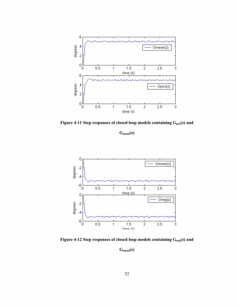
In the beginning of this section it is said that a single model transfer function is
going to be used and a controller is designed for the model containing this transfer
function and it is added that designed controller will be confirmed to be working
with the actual estimated transfer functions. Figure 4-11 and Figure 4-12 show the
step responses of closed loop CAS models containing both, Gmean(z), Gpos(z) and
Gneg(z).
52
Figure 4-11 Step responses of closed loop models containing Gpos(z) and
Gmean(z)
Figure 4-12 Step responses of closed loop models containing Gneg(z) and
Gmean(z)

53
As can be seen from these plots, we can say that designed controller works well
with the actual estimated models too. Hence in the non-linear flight simulations,
Gmean(z) is going to be used.
4.3.2 Controller for Second PWM Scheme
The same controller structure, that is PI with rate feedback, is used in the second
PWM scheme too. In this PWM scheme mathematical model of the CAS is the one
that is given in Section 3.4.2., because this PWM scheme uses both pos-solenoid
and neg-solenoid valves together. This mathematical model is repeated below.
)971.0z969.1z)(9441.0z943.1z()9886.0z987.1z(z0084893.0)z(G 22
22
+−+−+−
= ( 4.4 )
Controller is designed by trial and error process, which is built in MATLAB and
shown below
Figure 4-13 Closed loop CAS model built in MATLAB

54
Figure 4-14 Inside of MATLAB controller block for second PWM scheme
Below figures show the response of this closed loop CAS model to step inputs with
different magnitudes and sine inputs.
Figure 4-15 Model response to step input with magnitude 8

55
Figure 4-16 Model response to step input with magnitude 5
Figure 4-17 Model response to step input with magnitude 2

56
Figure 4-18 Response of the model to the sine input with amplitude 8 and
frequency 1 Hz
Although step responses of the closed loop model seem to have large overshoot
when compared with the closed loop model of the previous PWM scheme, its
response to 1 Hz frequency sine input is much better. Because estimated CAS
model in the second PWM scheme has rather fast dynamics when compared with
the model used in the first PWM scheme.
57
CHAPTER 5
5 SEEKER MODEL
5.1 Introduction
Seeker is the part of a missile that is used for detection and tracking of the target,
and ASGM (Air to Surface Guided Munition) use laser seekers to get the relative
position information about the target with respect to the munition. In semi active
guidance system, target is illuminated by a laser source and the seeker, which then
guides the weapon to the target, detects reflected laser beam. To increase the field
of view, the gimbaled type seeker is used, which looks in the direction of the
velocity vector. Figure showing this concept is given below.
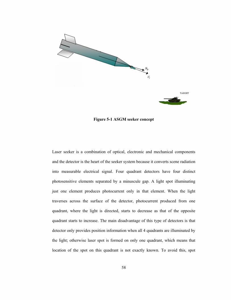
58
Figure 5-1 ASGM seeker concept
Laser seeker is a combination of optical, electronic and mechanical components
and the detector is the heart of the seeker system because it converts scene radiation
into measurable electrical signal. Four quadrant detectors have four distinct
photosensitive elements separated by a minuscule gap. A light spot illuminating
just one element produces photocurrent only in that element. When the light
traverses across the surface of the detector, photocurrent produced from one
quadrant, where the light is directed, starts to decrease as that of the opposite
quadrant starts to increase. The main disadvantage of this type of detectors is that
detector only provides position information when all 4 quadrants are illuminated by
the light; otherwise laser spot is formed on only one quadrant, which means that
location of the spot on this quadrant is not exactly known. To avoid this, spot

59
diameter should be at least equal to the detector radius, one of the ways of
achieving this spot size is defocusing.
We are going to generate a model for seeker, which processes the detector output
and extract the angle information from it. Processing the detector outputs, which
are 4 voltage values corresponding to each quadrant, to obtain the laser spot
location is the first step in the modeling studies. Second step is estimating the error
angle, whose definition is made in the next section, using spot location information
and some additional information about the configuration of detector and lens.
These can be better understood from Figure 5-2. Error angle estimation can be
obtained from geometry and optics, whereas spot location estimation, from detector
voltages, requires to be formed a more difficult relationship. In this chapter, first
we are going to explain how the error angle is estimated, once we know the laser
spot center location. Next we are going to give the usual and most frequently used
method of spot center estimation. After this, spot center estimation using artificial
neural network is introduced and explained. Finally results of these two methods
will be examined.

60
Figure 5-2 Seeker model block schema
5.2 Relation of the Spot Location with the Error Angle
Error angles are formed between LOS (Line of Sight) vector and velocity vector
(because seeker looks in the direction of velocity) in two planes namely pitch and
yaw planes. Let us call these angles pγ and Yγ , for pitch and yaw planes,
respectively. Estimation of these angles is based on the fact that, ray of light
passing the lens from its center doesn’t bend. Moreover it forms the center of the
laser spot. Hence if we know the distance of detector to the lens and if we can
estimate the spot center location, we can estimate the error angles by the following
expressions. This is illustrated in Figure 5-3 for pitch plane only.
⎟⎠⎞
⎜⎝⎛ ∆
=γdytanap ( 5.1 )
Detector
Voltages
(S1,S2,S3,S4)
Seeker Model
Part 1
Seeker Model
Part 2
Laser Spot
Location
(Xpos, Ypos)
Error
Angles
(γp, γy)
SEEKER MODEL

61
⎟⎠⎞
⎜⎝⎛ ∆
=γdxtanay ( 5.2 )
Figure 5-3 Lens and detector configuration and pitch plane error angle
5.3 Estimation of Spot Location
First of all we assume that laser spot is circular with radius r being equal to half of
the radius of the detector. Next we assume that 4 area values can be used instead of
4 voltage values, which are calculated using geometry once the spot center location
is given. Usage of areas instead of voltages doesn’t alter the results of estimation
methods because both methods use the normalized voltages (or areas).
The location of the center of the spot is determined with the following formula in
most of the applications, which is an approximation to the actual relationship
∆y
d
γp x
y
x
y Detector
Lens

62
between the amount of shift in the voltages and the amount of shift in the spot
center location [7]. Figure 5-4 shows the area values if the spot center location is
Xpos and Ypos.
4321
4321 )()(SSSSSSSSX pos +++
+−+= ( 5.3 )
4321
3241 )()(SSSSSSSSYpos +++
+−+= ( 5.4 )
Figure 5-4 Seeker spot position
The problem with this formula is that as the spot center goes far away from the
detector center, the error in spot center estimation increases. A primary aim is to
find a better relationship that works well for all possible spot center points. Also it
would be good to observe the performance of the ASGM under different seeker
models. Therefore an artificial neural network model is suggested, whose structure
is explained in the following sections.
S1S4
S3
S2
xpos
ypos

63
5.3.1 Artificial Neural Networks
Biologists have studied biological neural networks for many years. As information
about the functions of the brain was accumulated, a new technology emerged and
the quest for an artificial neural network started [5]. Neural Networks are
composed of simple elements operating in parallel. As in nature, the network
function is determined largely by the connections between elements. We can train a
neural network to perform a particular function by adjusting the values of
connections between elements [6].
In this thesis we have used radial basis neural network structure with two layers
because they are introduced for the solution of the real multivariable interpolation
problems like we have here. Our aim is to find a function taking the detector values
as input arguments and outputting the spot center location. Below is the schematic
of the two layer radial basis network structure.
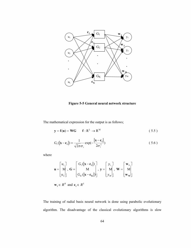
64
Figure 5-5 General neural network structure
The mathematical expression for the output is as follows;
ML RR: )( →== fWGufy ( 5.5 )
)2
exp(21)( 2
iiiG
σσπi
i
cxcx
−−=− ( 5.6 )
where
⎥⎥⎥
⎦
⎤
⎢⎢⎢
⎣
⎡=
Lu
uΜ1
u , ⎥⎥⎥
⎦
⎤
⎢⎢⎢
⎣
⎡
−
−=
)(
)(1
K
1
cx
cxG
KG
GΜ ,
⎥⎥⎥
⎦
⎤
⎢⎢⎢
⎣
⎡=
My
yΜ1
y , ⎥⎥⎥
⎦
⎤
⎢⎢⎢
⎣
⎡=
M
1
w
wW Μ
KR∈iw and LR∈ic
The training of radial basis neural network is done using parabolic evolutionary
algorithm. The disadvantage of the classical evolutionary algorithms is slow
u1
G1
G2
GK
.
.
u2
uL
y1
y2
1w1c
2c
Kc
.
.
yM
.
.
2w
Mw
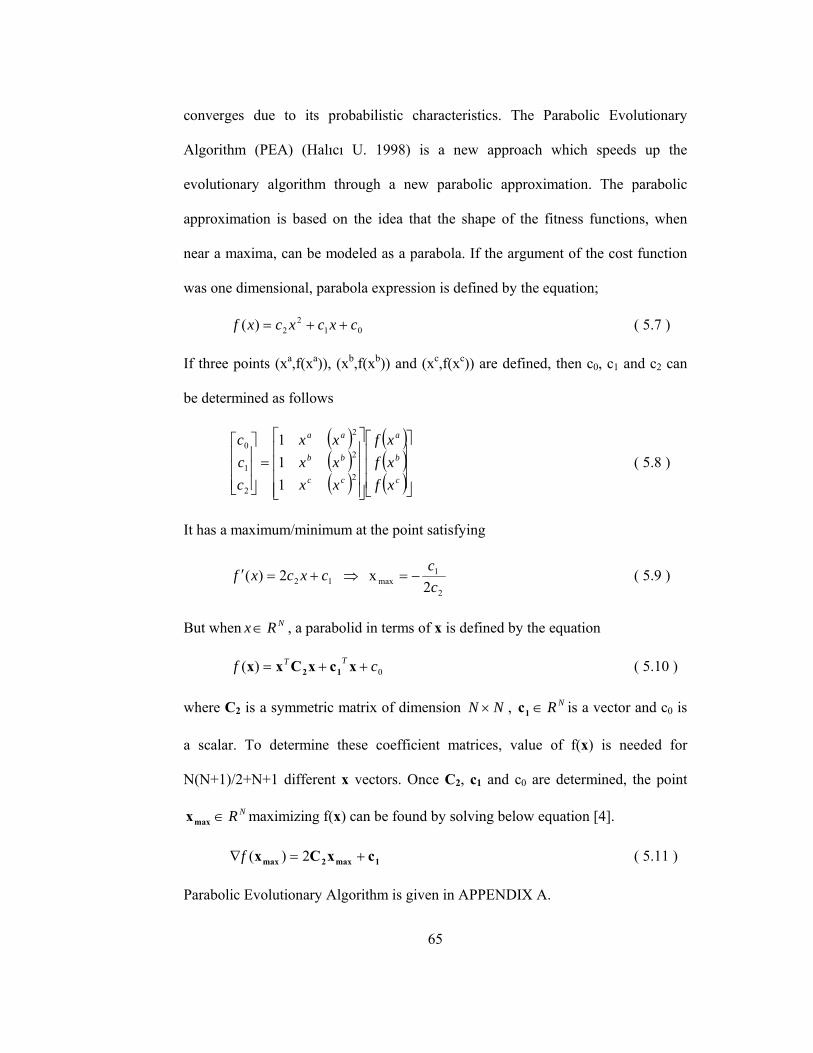
65
converges due to its probabilistic characteristics. The Parabolic Evolutionary
Algorithm (PEA) (Halıcı U. 1998) is a new approach which speeds up the
evolutionary algorithm through a new parabolic approximation. The parabolic
approximation is based on the idea that the shape of the fitness functions, when
near a maxima, can be modeled as a parabola. If the argument of the cost function
was one dimensional, parabola expression is defined by the equation;
012
2)( cxcxcxf ++= ( 5.7 )
If three points (xa,f(xa)), (xb,f(xb)) and (xc,f(xc)) are defined, then c0, c1 and c2 can
be determined as follows
( )( )( )
( )( )( )⎥
⎥⎥
⎦
⎤
⎢⎢⎢
⎣
⎡
⎥⎥⎥⎥
⎦
⎤
⎢⎢⎢⎢
⎣
⎡
=⎥⎥⎥
⎦
⎤
⎢⎢⎢
⎣
⎡
c
b
a
cc
bb
aa
xfxfxf
xxxxxx
ccc
2
2
2
2
1
0
111
( 5.8 )
It has a maximum/minimum at the point satisfying
2
1max12 2
x 2)(cc
cxcxf −=⇒+=′ ( 5.9 )
But when NRx ∈ , a parabolid in terms of x is defined by the equation
0)( cf TT ++= xcxCxx 12 ( 5.10 )
where C2 is a symmetric matrix of dimension NN × , NR∈1c is a vector and c0 is
a scalar. To determine these coefficient matrices, value of f(x) is needed for
N(N+1)/2+N+1 different x vectors. Once C2, c1 and c0 are determined, the point
NR∈maxx maximizing f(x) can be found by solving below equation [4].
1max2max cxCx +=∇ 2)(f ( 5.11 )
Parabolic Evolutionary Algorithm is given in APPENDIX A.
66
5.3.2 Determination of Training Data Set
Input and output of the ANN (Artificial Neural Network) model is 4 area values
and, X and Y components of spot center location. Hence training data set must be
composed of some input values and corresponding output values. If the input points
cover the input space uniformly, the success of learning the relationship between
inputs and outputs will be almost the same. However in our case, input-output pairs
are created using the expressions given below and the input of these expressions
are the outputs of the neural network, namely Xpos and Ypos. Therefore we can only
select output points, Xpos and Ypos, covering output space uniformly, the spread of
input points doesn’t have to be uniform. Hence, a training data set is created with
more data than required for training most probably. In other words, created training
data set is possibly overdetermined.

67
Figure 5-6 Detector spot area schematic
( ) ( )
pospospos
pos
pospos
pospos
yxy
yr
ryarxxrrxarrS
+−+
+−++=
2
sin22
sin24
22
222
22
1 π ( 5.12 )
( ) ( )
pospospos
pos
pospos
pospos
yxy
yr
ryarxxrrxarrS
−−−
−−++=
2
sin22
sin24
22
222
22
2 π ( 5.13 )
Xpos
ypos
r
β
α
Dedector
Laser
Spot
S1
S2 S3
S4
68
( ) ( )
pospospos
pos
pospos
pospos
yxy
yr
ryarxxrrxarrS
+−−
−−−−=
2
sin22
sin24
22
222
22
3 π ( 5.14 )
( ) ( )
pospospos
pos
pospos
pospos
yxy
yr
ryarxxrrxarrS
−−+
+−−−=
2
sin22
sin24
22
222
22
4 π ( 5.15 )
where “r” is the spot radius. Equations given above are obtained using geometry. In
the light of above explanations, uniformly spread output points (spot location
values) are picked and corresponding input values (4 area values) are estimated.
Since the possible spot center locations make a circle with the radius half of the
detector radius, training data set must be formed by selecting many Xpos and Ypos
values in this circle and estimating the areas corresponding to these locations. In
this way 221 input-output pair is created in order to train the radial basis neural
network.
5.4 Results of the Radial Basis Neural Network Model of Seeker
Neural Network model of the seeker is formed by using two layers and 4 neurons.
The schema of the model is given below.
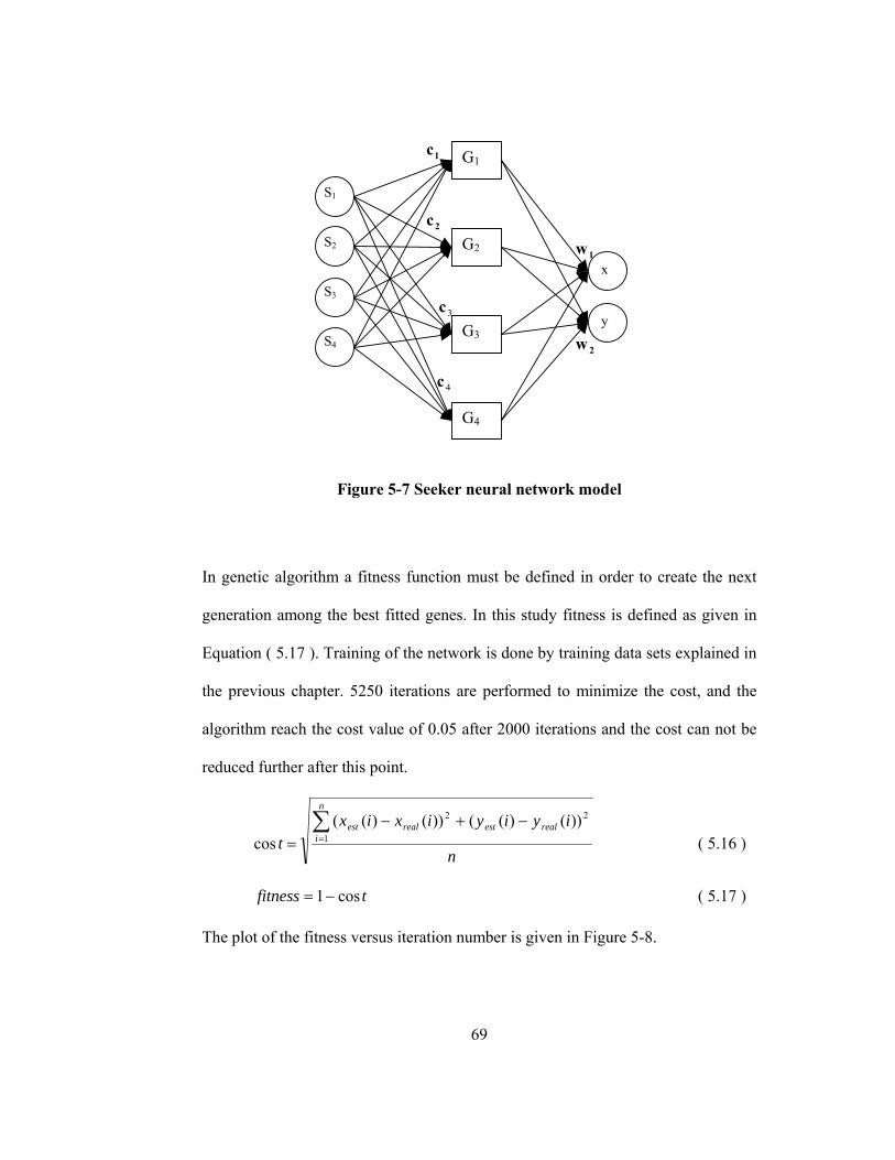
69
Figure 5-7 Seeker neural network model
In genetic algorithm a fitness function must be defined in order to create the next
generation among the best fitted genes. In this study fitness is defined as given in
Equation ( 5.17 ). Training of the network is done by training data sets explained in
the previous chapter. 5250 iterations are performed to minimize the cost, and the
algorithm reach the cost value of 0.05 after 2000 iterations and the cost can not be
reduced further after this point.
n
iyiyixixt
n
irealestrealest∑
=
−+−= 1
22 ))()(())()((cos ( 5.16 )
tfitness cos1−= ( 5.17 )
The plot of the fitness versus iteration number is given in Figure 5-8.
S1
G1
G2
G3
x
y
1w
1c
2c
3c
S2
2w
S3
S4
G4
4c
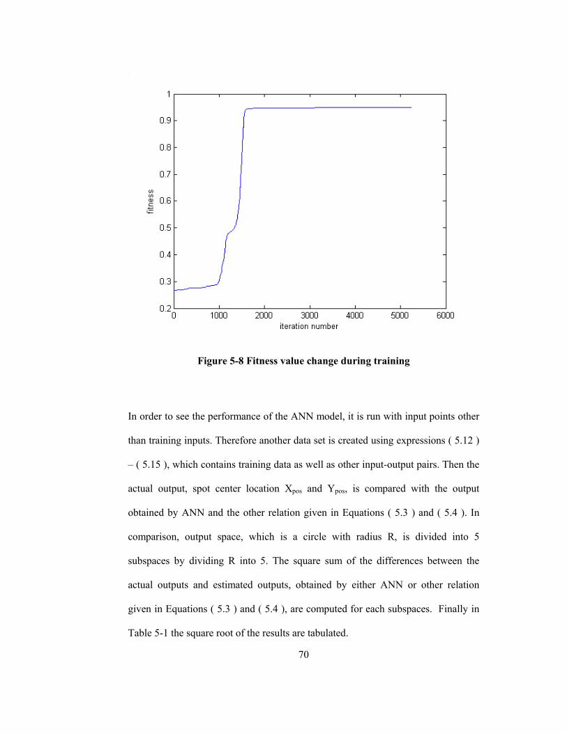
70
Figure 5-8 Fitness value change during training
In order to see the performance of the ANN model, it is run with input points other
than training inputs. Therefore another data set is created using expressions ( 5.12 )
– ( 5.15 ), which contains training data as well as other input-output pairs. Then the
actual output, spot center location Xpos and Ypos, is compared with the output
obtained by ANN and the other relation given in Equations ( 5.3 ) and ( 5.4 ). In
comparison, output space, which is a circle with radius R, is divided into 5
subspaces by dividing R into 5. The square sum of the differences between the
actual outputs and estimated outputs, obtained by either ANN or other relation
given in Equations ( 5.3 ) and ( 5.4 ), are computed for each subspaces. Finally in
Table 5-1 the square root of the results are tabulated.
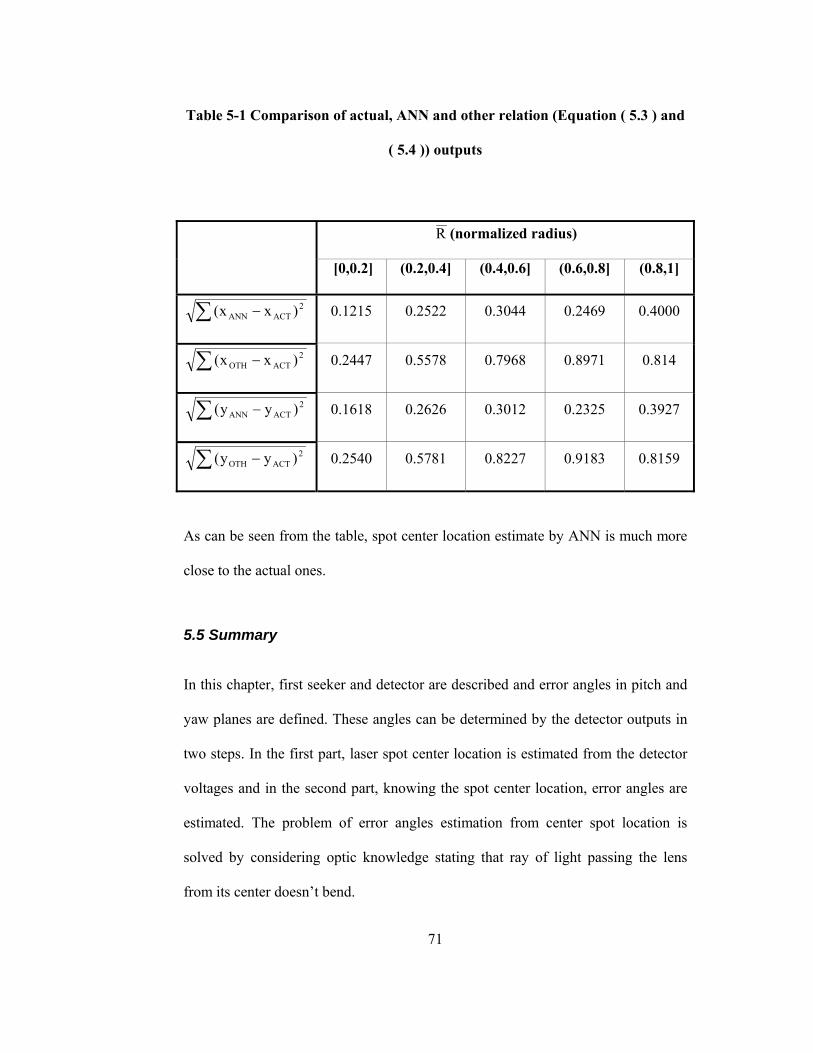
71
Table 5-1 Comparison of actual, ANN and other relation (Equation ( 5.3 ) and
( 5.4 )) outputs
R (normalized radius)
[0,0.2] (0.2,0.4] (0.4,0.6] (0.6,0.8] (0.8,1]
∑ − 2ACTANN )xx( 0.1215 0.2522 0.3044 0.2469 0.4000
∑ − 2ACTOTH )xx( 0.2447 0.5578 0.7968 0.8971 0.814
∑ − 2ACTANN )yy( 0.1618 0.2626 0.3012 0.2325 0.3927
∑ − 2ACTOTH )yy( 0.2540 0.5781 0.8227 0.9183 0.8159
As can be seen from the table, spot center location estimate by ANN is much more
close to the actual ones.
5.5 Summary
In this chapter, first seeker and detector are described and error angles in pitch and
yaw planes are defined. These angles can be determined by the detector outputs in
two steps. In the first part, laser spot center location is estimated from the detector
voltages and in the second part, knowing the spot center location, error angles are
estimated. The problem of error angles estimation from center spot location is
solved by considering optic knowledge stating that ray of light passing the lens
from its center doesn’t bend.
72
The estimation of spot center location from detector voltages are separately
examined. There already exists a relationship given in Equations ( 5.3 ) and ( 5.4 ),
but its success, as the spot center goes far away from the detector center, decreases.
Therefore an ANN estimation model is suggested instead of them. After the ANN
has learnt the relationship, its success is compared with the other equations taking
the actual values as basis. It is seen that the amount of error in ANN estimates are
smaller than that of the other equations. However more meaningful results about
the success of the seeker model will be obtained, when both ANN and other
relationships are placed in 6 degree of freedom simulations.

73
CHAPTER 6
6 OVERALL ASGM MATHEMATICAL MODEL
6.1 Introduction
After we worked on seeker and CAS units of the munition, a controller for the
munition is left to be designed. Since no sensors like accelerometers or gyros are
included in the munition, some common autopilots, such as acceleration autopilot,
can not be designed. However we can design a controller built on error angles
estimated by seeker unit and in this situation fuzzy control could be a good
solution. In this chapter first a brief introduction to fuzzy control will be given and
designed fuzzy control will be described. Afterwards overall ASGM model will be
explained with the input and output signal definition of each block (CAS block for
example) built in MATLAB Simulink.
6.2 Fuzzy Logic Control for Missile
6.2.1 What is Fuzzy Logic Control
The concept of Fuzzy Logic (FL) was conceived by Lotfi Zadeh, a professor at the
University of California at Berkley, and presented not as a control methodology,

74
but as a way of processing data by allowing partial set membership rather than
crisp set membership or non-membership. Professor Zadeh reasoned that people do
not require precise, numerical information input, and yet they are capable of highly
adaptive control. If feedback controllers could be programmed to accept noisy,
imprecise input, they would be much more effective and perhaps easier to
implement.
In this context, FL is a problem-solving control system methodology that lends
itself to implementation in systems ranging from simple, small, embedded micro-
controllers to large, networked, multi-channel PC or workstation-based data
acquisition and control systems. It can be implemented in hardware, software, or a
combination of both. FL provides a simple way to arrive at a definite conclusion
based upon vague, ambiguous, imprecise, noisy, or missing input information. FL's
approach to control problems mimics how a person would make decisions, only
much faster [18].
The fuzzy controller is composed of four main components called fuzzification,
inference, knowledge base and defuzzification shown as in Figure 6-1.
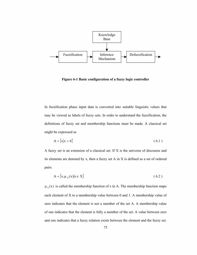
75
Figure 6-1 Basic configuration of a fuzzy logic controller
In fuzzification phase input data is converted into suitable linguistic values that
may be viewed as labels of fuzzy sets. In order to understand the fuzzification, the
definitions of fuzzy set and membership functions must be made. A classical set
might be expressed as
6xxA >= ( 6.1 )
A fuzzy set is an extension of a classical set. If X is the universe of discourse and
its elements are denoted by x, then a fuzzy set A in X is defined as a set of ordered
pairs.
Xx)x(,xA A ∈µ= ( 6.2 )
)x(Aµ is called the membership function of x in A. The membership function maps
each element of X to a membership value between 0 and 1. A membership value of
zero indicates that the element is not a member of the set A. A membership value
of one indicates that the element is fully a member of the set. A value between zero
and one indicates that a fuzzy relation exists between the element and the fuzzy set.
Fuzzification Inference Mechanism
Defuzzification
Knowledge Base
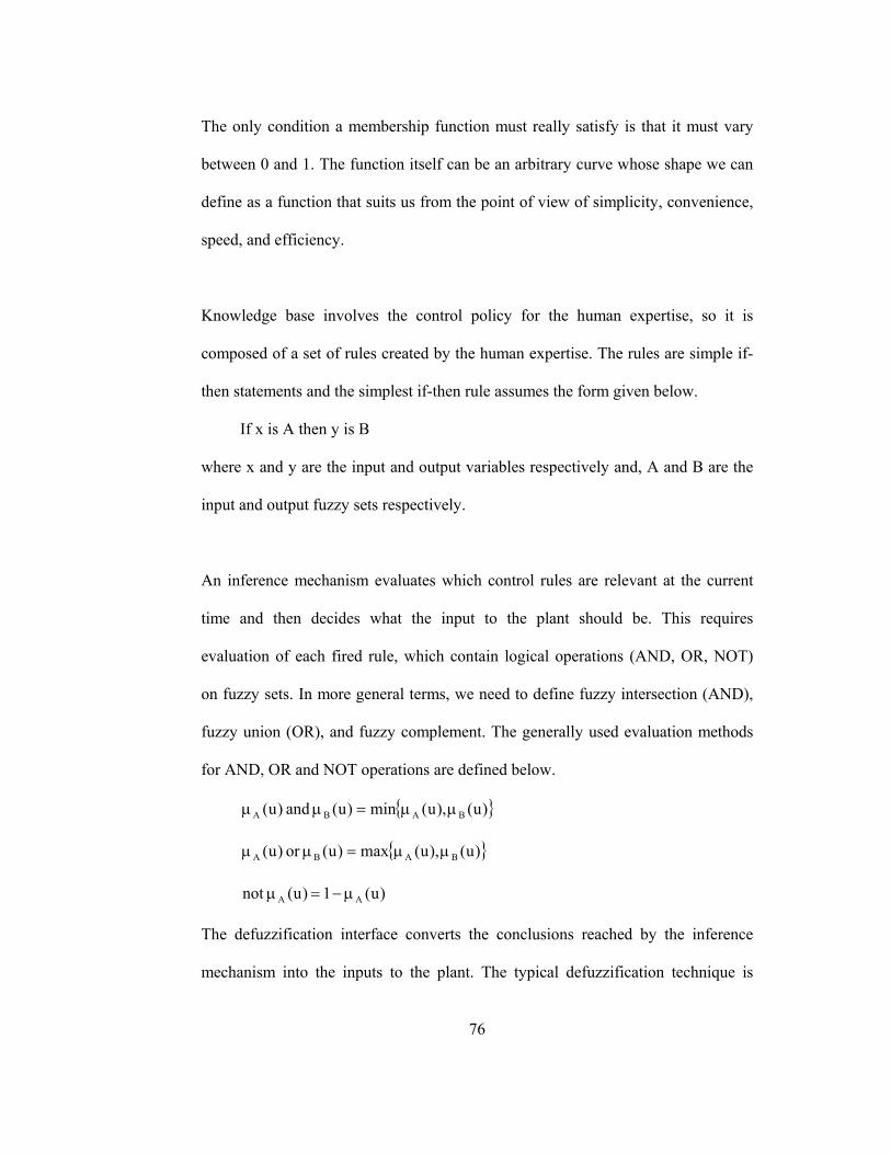
76
The only condition a membership function must really satisfy is that it must vary
between 0 and 1. The function itself can be an arbitrary curve whose shape we can
define as a function that suits us from the point of view of simplicity, convenience,
speed, and efficiency.
Knowledge base involves the control policy for the human expertise, so it is
composed of a set of rules created by the human expertise. The rules are simple if-
then statements and the simplest if-then rule assumes the form given below.
If x is A then y is B
where x and y are the input and output variables respectively and, A and B are the
input and output fuzzy sets respectively.
An inference mechanism evaluates which control rules are relevant at the current
time and then decides what the input to the plant should be. This requires
evaluation of each fired rule, which contain logical operations (AND, OR, NOT)
on fuzzy sets. In more general terms, we need to define fuzzy intersection (AND),
fuzzy union (OR), and fuzzy complement. The generally used evaluation methods
for AND, OR and NOT operations are defined below.
)u(),u(min)u( and )u( BABA µµ=µµ
)u(),u(max)u(or )u( BABA µµ=µµ
)u(1 )u( not AA µ−=µ
The defuzzification interface converts the conclusions reached by the inference
mechanism into the inputs to the plant. The typical defuzzification technique is
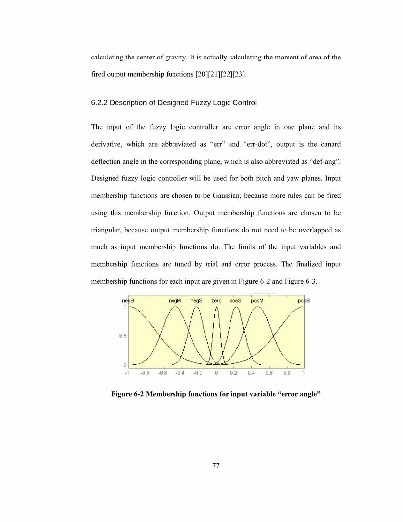
77
calculating the center of gravity. It is actually calculating the moment of area of the
fired output membership functions [20][21][22][23].
6.2.2 Description of Designed Fuzzy Logic Control
The input of the fuzzy logic controller are error angle in one plane and its
derivative, which are abbreviated as “err” and “err-dot”, output is the canard
deflection angle in the corresponding plane, which is also abbreviated as “def-ang”.
Designed fuzzy logic controller will be used for both pitch and yaw planes. Input
membership functions are chosen to be Gaussian, because more rules can be fired
using this membership function. Output membership functions are chosen to be
triangular, because output membership functions do not need to be overlapped as
much as input membership functions do. The limits of the input variables and
membership functions are tuned by trial and error process. The finalized input
membership functions for each input are given in Figure 6-2 and Figure 6-3.
Figure 6-2 Membership functions for input variable “error angle”

78
Figure 6-3 Membership functions for input variable “error angle derivative”
The long forms of linguistic abbreviations used in these figures are given below.
negB: Negative Big
negM: Negative Medium
negS: Negative Small
zero: Zero
posS: Positive Small
posM: Positive Medium
posB: Positive Big
The membership functions of the output variables are given in Figure 6-4.
Figure 6-4 Membership functions for output variable “canard deflection”

79
The rule base of the fuzzy logic control for this ASGM is given in Table 6-1.
Table 6-1 Rule-base for ASGM
“err” “def-ang”
negB negM negS Zero posS posM posB
negB negB negB negB negM negM negS zero
negM negB negB negM negM negS zero posS
negS negB negM negM negS zero posS posM
zero negM negM negS Zero posS posM posM
posS negM negS zero posS posM posM posB
posM negS zero posS posM posM posB posB
“err
-dot
”
posB Zero posS posM posM posB posB posB
This table is read as given in the following example: “If err is negB and if err-dot is
negB, then def-ang is negB”. The logical operation “and” is evaluated as taking the
minimum and defuzzification method is calculating the center of gravity. The
mapping from inputs “err” and “err-dot” to output “def-ang” is shown as a surface
plot in Figure 6-5.
80
Figure 6-5 Input-Output mapping of the fuzzy logic controller
6.3 Integration of CAS and Seeker Models to the Non-linear Flight
Model
Nonlinear flight simulations will be performed for bang-bang control and for
continuous control schemes separately, whose mathematical models are built in
MATLAB Simulink environment. Bang-bang controlled ASGM model contains
seeker model but do not include error angle estimations. The CAS plant used in
these simulations is the open loop CAS model given in Equation 4.3. ASGM model
with continuous control contains seeker model together with error angle
estimations using Artificial Neural Network approach, closed loop CAS models
obtained in Sections 4.3.1 and 4.3.2 and fuzzy logic controller. Simulation model
of bang-bang controlled ASGM is very straightforward, seeker determines the
direction of the target as right or left and up or down, therefore in the simulations
output of the seeker is 1 or -1. Output of the seeker directly enters the open-loop
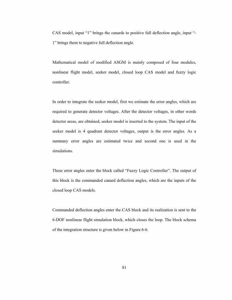
81
CAS model, input “1” brings the canards to positive full deflection angle, input “-
1” brings them to negative full deflection angle.
Mathematical model of modified ASGM is mainly composed of four modules,
nonlinear flight model, seeker model, closed loop CAS model and fuzzy logic
controller.
In order to integrate the seeker model, first we estimate the error angles, which are
required to generate detector voltages. After the detector voltages, in other words
detector areas, are obtained, seeker model is inserted to the system. The input of the
seeker model is 4 quadrant detector voltages, output is the error angles. As a
summary error angles are estimated twice and second one is used in the
simulations.
These error angles enter the block called “Fuzzy Logic Controller”. The output of
this block is the commanded canard deflection angles, which are the inputs of the
closed loop CAS models.
Commanded deflection angles enter the CAS block and its realization is sent to the
6-DOF nonlinear flight simulation block, which closes the loop. The block schema
of the integration structure is given below in Figure 6-6.

82
Figure 6-6 Block schema of the integrated munition system
Non-linear flight
Simulation Model
Seeker
γp γy
y
p
ˆ
ˆ
γ
γFuzzy Controller
CAS
δe-com δr-com
δe-real δr-real

83
CHAPTER 7
7 SIMULATION STUDIES
7.1 Introduction
Simulation studies are carried out in order to see the success of the modifications
made on ASGM. Comparison is made between the hit accuracy of bang-bang
control scheme and continuous control scheme with modified CAS, seeker units
and fuzzy logic controller.
7.2 Simulation Scenarios
7.2.1 Scenario 1
In this scenario, ASGM is fired onto a stationary target, which is aligned with the
ASGM in x-z plane (pitch plane). The initial state values of ASGM and location of
target is summarized in Table 7-1.

84
Table 7-1 Initial state values of simulation and target location table for
Scenario 1
ASGM Initial Position Initial Attitude
x y z Φ θ Ψ 0 m 0 m -5000 m 0 deg -10 deg 0 deg
Initial velocity, α and β Initial Angular Rates Vt α β p q r
295 m/s 0 deg 0 deg 0 0 0 Target Location
x y z 8500 m 0 m 0
Below figures are drawn for three different configurations; first one is bang-bang,
second one is continuous control with fuzzy logic using CAS model with second
PWM scheme and the last configuration is again continuous control but with first
PWM scheme.
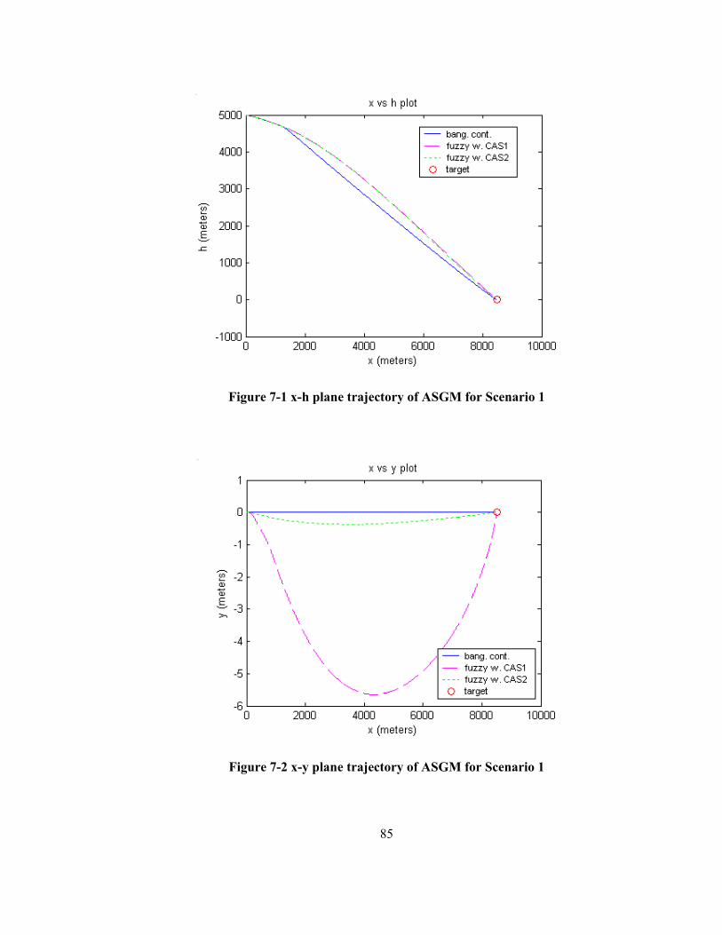
85
Figure 7-1 x-h plane trajectory of ASGM for Scenario 1
Figure 7-2 x-y plane trajectory of ASGM for Scenario 1

86
Figure 7-1 and Figure 7-2 show that all the configurations of ASGM hit the target
with a hit accuracy less than 10 meters, whose details are given in Table 7-2.
Interesting trajectory in x-y plane occurs due to continuous control. Because when
there is an error angle less than 1 degree, then there is no control action in bang-
bang control simulations. In other words this is zero region for bang-bang control
scheme. However in continuous control, any error angle no matter how small it is
causes CAS to be commanded to some angle. As a result this trajectory is observed
in x-y plane.
This can also be seen from Φ, θ and Ψ angle histories given in Figure 7-3. While
some little amount of Φ and Ψ angles are realized in continuous control scheme, in
bang-bang control scheme no Φ and Ψ angles are realized. In addition to this, with
continuous control scheme, large oscillations in pitch angle occurred (θ) with bang-
bang control scheme is overcome.
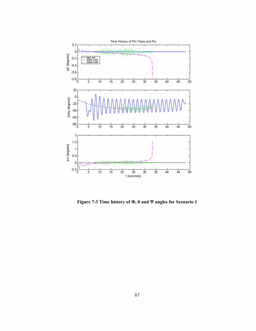
87
Figure 7-3 Time history of Φ, θ and Ψ angles for Scenario 1
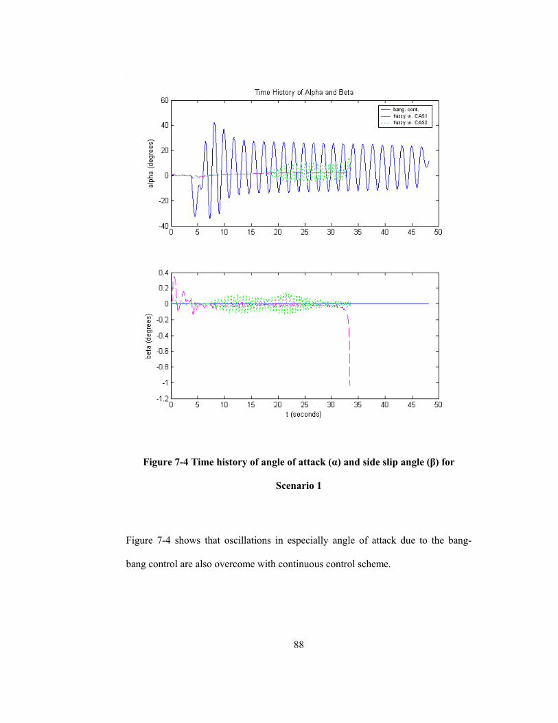
88
Figure 7-4 Time history of angle of attack (α) and side slip angle (β) for
Scenario 1
Figure 7-4 shows that oscillations in especially angle of attack due to the bang-
bang control are also overcome with continuous control scheme.
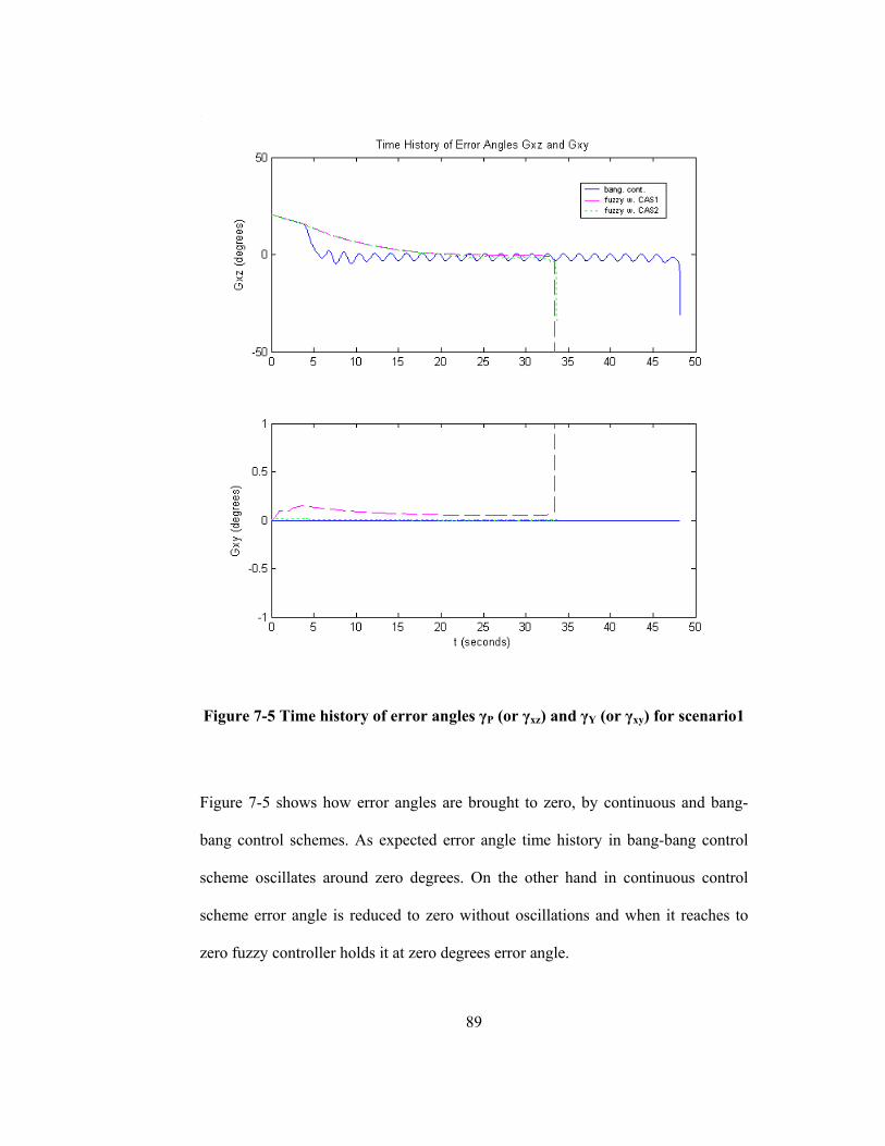
89
Figure 7-5 Time history of error angles γP (or γxz) and γY (or γxy) for scenario1
Figure 7-5 shows how error angles are brought to zero, by continuous and bang-
bang control schemes. As expected error angle time history in bang-bang control
scheme oscillates around zero degrees. On the other hand in continuous control
scheme error angle is reduced to zero without oscillations and when it reaches to
zero fuzzy controller holds it at zero degrees error angle.
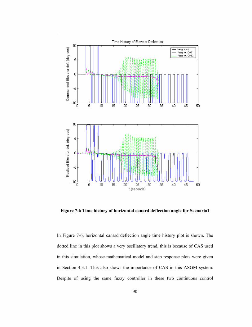
90
Figure 7-6 Time history of horizontal canard deflection angle for Scenario1
In Figure 7-6, horizontal canard deflection angle time history plot is shown. The
dotted line in this plot shows a very oscillatory trend, this is because of CAS used
in this simulation, whose mathematical model and step response plots were given
in Section 4.3.1. This also shows the importance of CAS in this ASGM system.
Despite of using the same fuzzy controller in these two continuous control

91
configuration, CAS models having different time domain characteristics, such as
settling time, response time etc, causes considerable changes in the behavior of
whole ASGM system.
Figure 7-7 Time history of vertical canard deflection angle for Scenario1
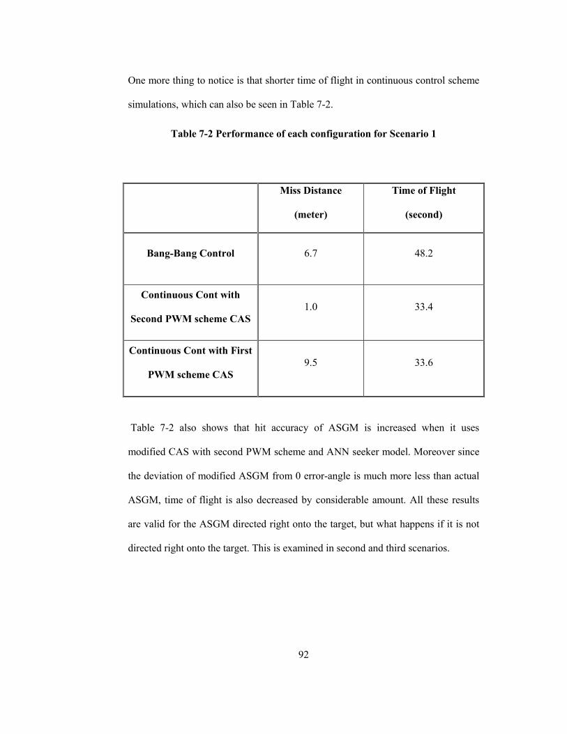
92
One more thing to notice is that shorter time of flight in continuous control scheme
simulations, which can also be seen in Table 7-2.
Table 7-2 Performance of each configuration for Scenario 1
Miss Distance
(meter)
Time of Flight
(second)
Bang-Bang Control 6.7 48.2
Continuous Cont with
Second PWM scheme CAS 1.0 33.4
Continuous Cont with First
PWM scheme CAS 9.5 33.6
Table 7-2 also shows that hit accuracy of ASGM is increased when it uses
modified CAS with second PWM scheme and ANN seeker model. Moreover since
the deviation of modified ASGM from 0 error-angle is much more less than actual
ASGM, time of flight is also decreased by considerable amount. All these results
are valid for the ASGM directed right onto the target, but what happens if it is not
directed right onto the target. This is examined in second and third scenarios.

93
7.2.2 Scenario 2
In this scenario, the location of the target is 8500 meters in x direction, 900 meters
in y direction and its height is 0 meter, whereas ASGM is fired from a height of
5000 meters. Initial condition of ASGM and location of stationary target is
summarized in Table 7-3.
Table 7-3 Initial state values of simulation and target location table for
Scenario 2
ASGM Initial Position Initial Attitude
x y z Φ θ Ψ 0 m 0 m -5000 m 0 deg -30 deg 5 deg
Initial Velocity, α and β Initial Angular Rates Vt α β p q r
295 m/s 0 deg 0 deg 0 0 0 Target Location
x y z 8500 m 900 m 0

94
Figure 7-8 x-h plane trajectory of ASGM for Scenario 2
Figure 7-9 x-y plane trajectory of ASGM for Scenario 2
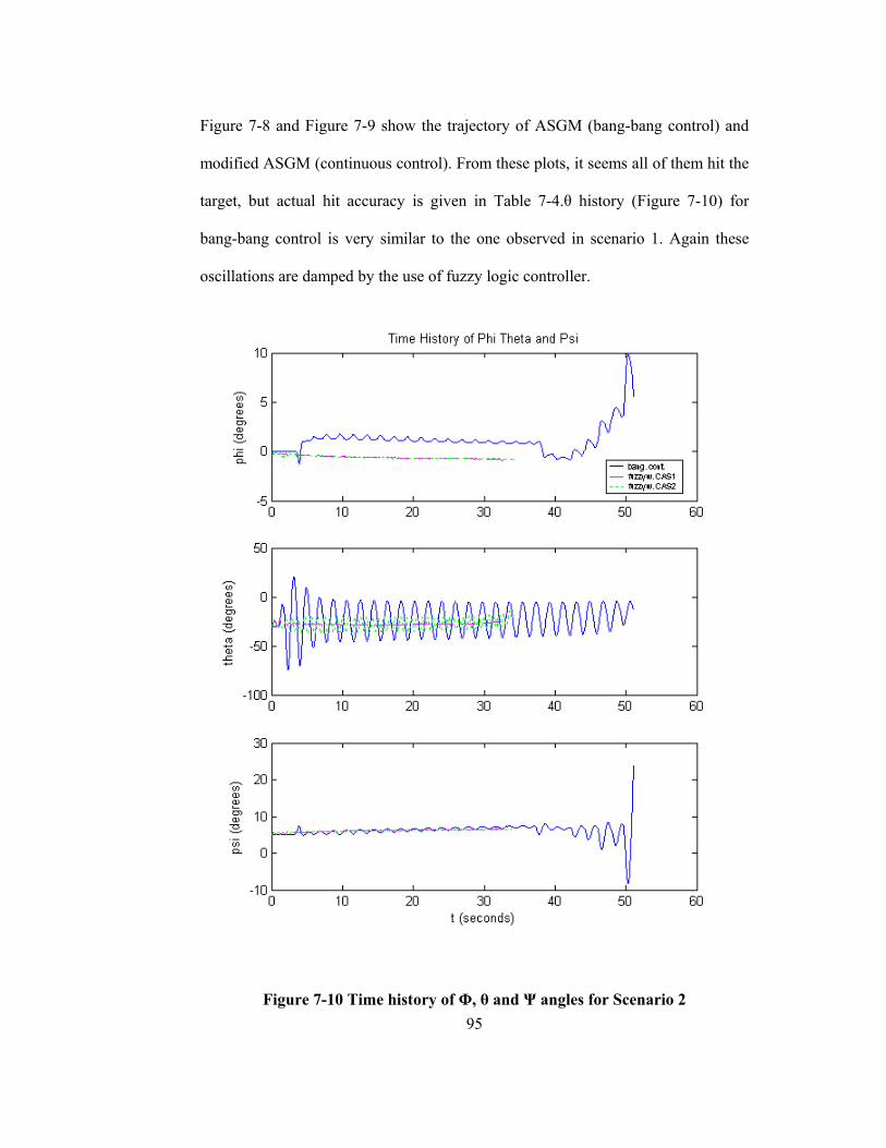
95
Figure 7-8 and Figure 7-9 show the trajectory of ASGM (bang-bang control) and
modified ASGM (continuous control). From these plots, it seems all of them hit the
target, but actual hit accuracy is given in Table 7-4.θ history (Figure 7-10) for
bang-bang control is very similar to the one observed in scenario 1. Again these
oscillations are damped by the use of fuzzy logic controller.
Figure 7-10 Time history of Φ, θ and Ψ angles for Scenario 2
96
Figure 7-11 Time history of angle of attack (α) and side slip angle (β) for
Scenario 2

97
As can be seen in Figure 7-11, in bang-bang control simulations, angle of attack
oscillates too much, and these oscillations are removed by the use of fuzzy logic
control.
Figure 7-12 Time history of error angles γP (or γxz) and γY (or γxy) for
scenario2

98
Figure 7-12 shows the success of the continuous control when compared with the
bang-bang control, because bang-bang control causes munition to oscillate around
zero error angle, whereas in continuous control case once it is brought to zero error
angle, it is held at this position without oscillations.
Figure 7-13 Time history of horizontal canard deflection angle for Scenario2

99
In Figure 7-13 resultant horizontal canard deflection of bang-bang control
simulations are obvious, but there is one more horizontal canard angle history that
oscillates much, too. This angle history is the result of continuous control with first
PWM scheme CAS. This is because CAS itself has a very oscillatory response,
which can be seen in Section 4.3.1.
100
Figure 7-14 Time history of vertical canard deflection angle for Scenario2
Since error angle in x-y plane is very small, small vertical canard deflections would
be enough to steer the munition. This fact is realized in bang-bang control
101
simulation as most of the time zero vertical canard deflection and several times full
deflection commands for a little time.
Table 7-4 Performance of each configuration for Scenario 2
Miss Distance
(meter)
Time of Flight
(second)
Bang-Bang Control 15.8 51.1
Continuous Cont with
Second PWM scheme CAS 1.9 33.2
Continuous Cont with First
PWM scheme CAS 12.8 34.3
Table 7-4 summarizes the performance of bang-bang control and continuous
control scheme. According to this table, as expected, ASGM with fuzzy logic
controller using second PWM scheme hits the target with accuracy less than 2
meters. The unsatisfactory performance of continuous control using first PWM
scheme is due to insufficient closed loop performance of CAS. In the third scenario
effect of initial large error angle will be examined.
102
7.2.3 Scenario 3
In scenario 3, the location of target is not altered, but ASGM has different
orientation than the second scenario. Initial state values and target location are
given in Table 7-5.
Table 7-5 Initial state values of simulation and target location table for
Scenario 3
ASGM Initial Position Initial Attitude
x y z Φ θ Ψ 0 m 0 m -5000 m 0 deg -10 deg 0 deg
Initial velocity, α and β Initial Angular Rates Vt α β p q r
295 m/s 0 deg 0 deg 0 0 0 Target Location
x y z 8500 m 900 m 0
In this scenario, bang-bang controlled ASGM loses the acquisition with the target
after some time, which can be seen in Figure 7-15 and Figure 7-16.
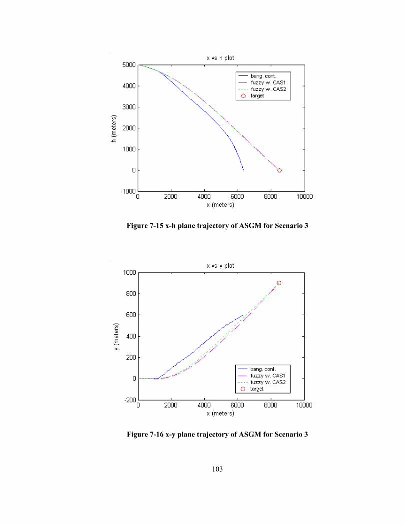
103
Figure 7-15 x-h plane trajectory of ASGM for Scenario 3
Figure 7-16 x-y plane trajectory of ASGM for Scenario 3

104
Figure 7-17 Time history of Φ, θ and Ψ angles for scenario 3
Figure 7-17 shows that due to full horizontal canard and vertical canard deflections
in bang-bang control scheme, munition attains large roll angles, but this doesn’t
create a problem in controlling point of view. Because borders, which separate the
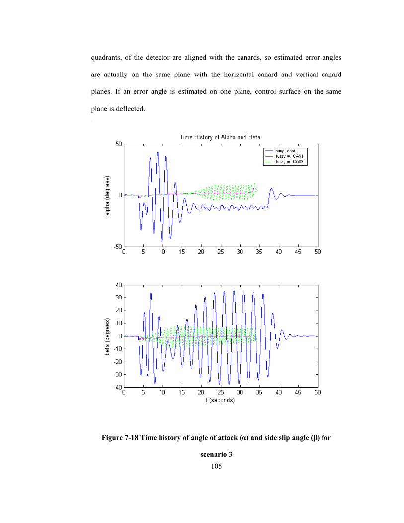
105
quadrants, of the detector are aligned with the canards, so estimated error angles
are actually on the same plane with the horizontal canard and vertical canard
planes. If an error angle is estimated on one plane, control surface on the same
plane is deflected.
Figure 7-18 Time history of angle of attack (α) and side slip angle (β) for
scenario 3
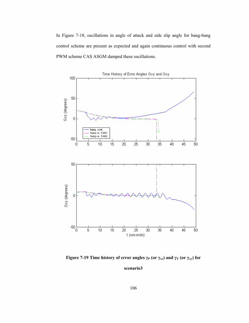
106
In Figure 7-18, oscillations in angle of attack and side slip angle for bang-bang
control scheme are present as expected and again continuous control with second
PWM scheme CAS ASGM damped these oscillations.
Figure 7-19 Time history of error angles γP (or γxz) and γY (or γxy) for
scenario3

107
Figure 7-19 shows the error angle history in both planes and demonstrates very
similar trend to the previous two scenarios. From these plots, the point where
acquisition starts and ends can also be found out, at around 36th second acquisition
is lost and flight is turned to ballistic flight in bang-bang controlled ASGM.
Accordingly vertical and horizontal canard defections are zero after this time,
which can be seen in Figure 7-19.

108
Figure 7-20 Time history of horizontal canard deflection angle for scenario 3

109
Figure 7-21 Time history of vertical canard deflection angle for scenario 3

110
Table 7-6 Performance of each configuration for scenario 3
Miss Distance
(meter)
Time of Flight
(second)
Bang-Bang Control - (acquisition lost) 49.3
Continuous Cont with
Second PWM scheme CAS 1.1 33.6
Continuous Cont with First
PWM scheme CAS 13.5 34.5
Table 7-6 indicates that when control algorithm is continuous and the performance
of CAS is satisfactory and compatible with the munition, the release envelope of
the munition can be enlarged.

111
CHAPTER 8
8 CONCLUSION
This thesis aims to improve the mentioned ASGM by modifying some of its
components to reduce miss distance. For this purpose, first seeker unit of ASGM
was modified then control actuation system was changed to the one that is
continuous. In other words, canards rotate to the desired deflection, not full
deflection.
Modification on seeker unit is made by changing the algorithm. Before
modification detector was used to decide on whether the target is up/below or
right/left of the munition, but with the modification the error angles can be
estimated now. Although there is a popular equation that is used to locate the laser
spot, for accuracy in estimation of the laser spot we suggested ANN seeker model
which estimated the laser spot location more accurately.
The major improvement is made on the control actuation system, because after the
modification it could operate continuously. Two mathematical models were

112
estimated using system identification, and they were used with two different PWM
schemes.
In order to see the effect of these improvements on the overall system, simulations
are performed for three scenarios. The first and second scenarios showed us that the
miss distance decreased to around 2 meters, whereas in bang-bang control it is
around 16 meters. Moreover time of flight value is decreased when compared with
the bang-bang controlled ASGM. However it is also seen that the oscillatory
characteristic of the first PWM scheme CAS increased the miss distance to a value
that could also be accomplished by bang-bang control. This showed us that the
performance of the CAS is as important as the performance of flight controller.
In the third scenario, it is shown that, modified ASGM has a larger delivery
envelope when compared with the bang-bang controlled ASGM. Because
acquisition with the target is lost after some time in this scenario, whereas
improved ASGM again hits the target with an accuracy of 1 meter.
Future studies could be building a nonlinear parametric model of CAS and
estimating the unknown parameters of this model, because it is difficult to fit a
linear mathematical model; as indicated in Chapter 3. Moreover, in order to damp
the oscillations, model predictive controller can be designed instead of PI with rate
feedback controller for the control actuation system.

113
REFERENCES
[1] Blakelock, J. H., “Automatic Control of Aircraft and Missiles”, John Wiley
& Sons Inc., 1991.
[2] McLean, D., “Automatic Flight Control Systems”, Prentice Hall
International (UK) Ltd., 1990.
[3] Roskam, J., “Airplane Flight Dynamics and Automatic Flight Controls”
DARcorporation, 1995.
[4] Halici U., Leblebicioğlu K., Jain L.C. “Training Radial Basis Function
Neural Networks Through Parabolic Evolutionary Algorithm” International
Journal of Knowledge-Based Intelligent Engineering Systems, Vol.5, No.3,
July 2001.
[5] Kartalopoulos, S. V., “Understanding Neural Networks and Fuzzy Logic:
Basic Concepts and Applications”, IEEE Press, 1996.
[6] MATLAB Neural Network Toolbox User Guide.
[7] UDT Instruments “Non-Contact Position Sensing Using Optical Detectors”
( www.udt.com ).
[8] Efe, M., “Laserle Aydınlatılmış Hedef Konumu Belirleme ve Hedefe
Kilitlenme”, Yüksek Lisans Tezi, Elektronik Mühendisliği Bölümü, Ankara
Üniversitesi, Ankara 1994.
[9] Ogata, K., “Modern Control Engineering”, Prentice Hall Inc., 1997.
[10] Sinha, N. K. and Kustza, B., “Modeling and Identification of Dynamic
Systems”, Van Nostrand Reinhold Co., 1983.
[11] MATLAB System Identification Toolbox User’s Guide.
[12] Özkan, A., “Development of a Control Actuation System for an Inertially
Guided Missile”, M.S. Thesis, Mechanical Engineering Department,
METU, Ankara, 1996.
114
[13] Perkgöz, C., “A Guidance and Control Method for a Tail Controlled
Bomb”, M.S. Thesis, Electrical and Electronics Engineering Department,
METU, Ankara, 2002.
[14] Ljung, L., “System Identification: Theory for the User”, P T R Prentice
Hall, Inc., 1987.
[15] Ateşoğlu, Ö., “Different Autopilot Designs Their Performance Comparison
For Guided Missiles” M.S. Thesis, Aeronautical Engineering Department,
METU, Ankara 1996.
[16] Hou, L. and Michel A. N. “Stability Analysis of Pulse-Width-Modulated
Feedback Systems”, Automatica, Vol.37, pp.1335-1349, 2001.
[17] van Varseveld, R. B. and Bone, G. M. “Accurate Position Control of a
Pneumatic Actuator Using On/Off Solenoid Valves”, IEEE/ASME
Transactions on Mechatronics, Vol.2, No.3, pp. 195-204, September 1997.
[18] Linnet, J.A. and Smith, M. C. “An Accurate Low Friction Pneumatic
Position Control System” Proceeding of the Institution of Mechanical
Engineers Part B, Vol.203, No.33, pp.159-165, April 1989.
[19] MATLAB Fuzzy Logic Toolbox User’s Guide.
[20] Lin, C. L. and Su, H. W., “Intelligent Control Theory in Guidance and
Control System Design: an Overview”, Proc. Natl. Sci. Counc. ROC(A),
Vol.24 No.1, pp.15-30, 2000.
[21] O’Hagan, M., “A Fuzzy Decision Maker”, ( www.fuzzysys.com )
[22] Passino, K. M., Yurkovich, S., “Fuzzy Control” Addison Wesley Longman
Inc., 1998.
[23] Vural, A. Ö., “Fuzzy Logic Guidance System Design for Guided Missiles”
M.S. Thesis, Mechanical Engineering Department, METU, Ankara, 2003.
[24] Jamshidi, M., Vadiee, N. and Ross, T, “Fuzzy Logic and Control” PTR
Prentice Hall, Inc., 1993.
[25] Rajasekhar V. and Sreenatha A. G. “Fuzzy Logic Implementation of
Proportional Navigation Guidance” Acta Astronautica Vol.46, No.1, pp.17-
24, 2000.

115
[26] Ateşoglu, Ö. “Fuzzy Guidance and Control Inference Design for a Non-
linear Air to Surface Missile Model” Nordic Matlab Conference, pp.148-
154, 2001.

116
APPENDIX A
A PARABOLIC EVOLUTIONARY ALGORITHM
Initialize Population Gn=G0 with size(Gn)=P
repeat
• Mutation: Mutatate Gn except the best one considering mutation rate Mr • Breeding: Generate temporary population Gt through parabolic crossover and classical
crossover such that size(Gt)=P+2*⎡P*Cr⎤
• Parabolic crossover: L*3*N new chromosomes are generated for Gt as follows: repeat for loop=1..L
• select three vectors xa, xb, xc from Gn in random (however for a predetermined ratio, xa is not selected in random but set to xbest in Gn)
• repeat for i=1..N
• determine (xi)a
max using three pairs
(xai,fa(xa
i)), (xbi,fa(xb
i)), (xci,fa(xc
i));
(xi)bmax using three pairs
(xai,fb(xa
i)), (xbi,fb(xb
i)), (xci,fb(xc
i));
(xi)cmax using three pairs
(xai,fc(xa
i)), (xbi,fc(xb
i)), (xci,fc(xc
i));
where xai, xb
i and xci are the ith compenent of the vectors xa, xb and xc respectively,
• add x(xa,xi)max=x(xa,(xi)a
max),
x(xb,xi)max=x(xb,(xi)bmax),

117
x(xc,xi)max=x(xc,(xi)cmax) to Gt
• Classical Crossover: Generate 2*⎡P*Cr⎤ - L*3*N chromosomes through classical two point crossover and add them to temporary population Gt in addition to Gn,
• Selection: Select P-1 chromosomes from Gt by roulette-wheel rule and add the best chromosomes
of Gt to generate Gn+1 until Stopping Condition S(Gn+1) is satisfied

118
APPENDIX B
B ANGLE MEASUREMENT DEVICES
Two angle sensors are used in the test setup: Encoder (Heidenhain ROC 417) and
arc segment potentiometer. ROC 417 is an absolute, single turn rotary encoder with
its own bearing, whose picture is given in Figure B-1. It has both incremental and
absolute angle measurement. It has 8192 line counts that are used for its
incremental measurements. Absolute signals are digital with 17 bits in EnDat
(Encoder Data) data format. EnDat interface makes it possible to transmit position
values as well as parameters (e.g. datum shift) quickly and reliably with only 4
signal lines. However extracting the position data from the encoder requires
designing an electronic card, which sends the clock and mod signals and receives
position data. This card is also designed, manufactured and tested.
Figure B-1 Heidenhain ROC 417 encoder

119
Summary of its specifications are also given in Table B-1.
Table B-1 ROC 417 encoder specifications
ROC 417
Incremental Signals 1 VPP (Sine shape signal)
Line Counts 8192
Absolute position values EnDat
Positions/rev. 131072 (17 bits)
Power supply 5 V
Operating temperature Max. 80 ˚C
Arc segment potentiometer is the other angle sensor, whose drawing is given in
Figure B-2.
Figure B-2 Drawing of arc segment potentiometer
Its arc shape makes it special for applications which don’t have full rotation, like in
the fin actuation systems. In this way less space is occupied by the angle sensors.
Its specifications are given in Table B-2.
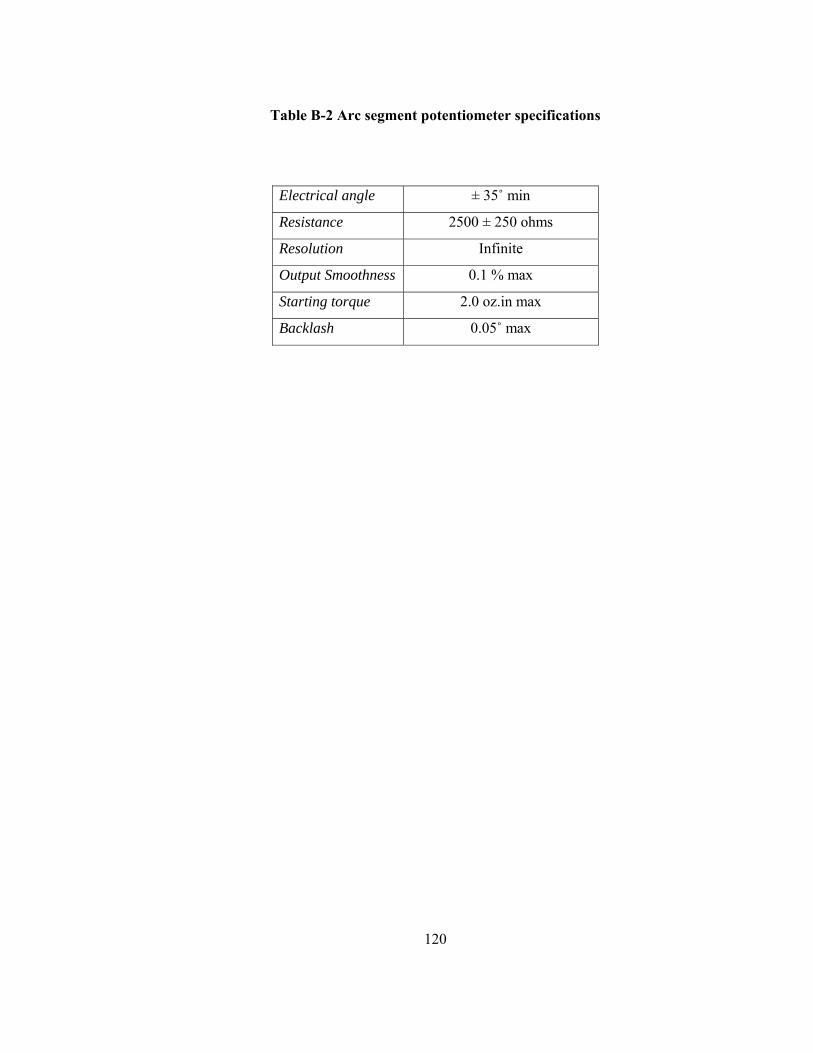
120
Table B-2 Arc segment potentiometer specifications
Electrical angle ± 35˚ min
Resistance 2500 ± 250 ohms
Resolution Infinite
Output Smoothness 0.1 % max
Starting torque 2.0 oz.in max
Backlash 0.05˚ max


![Stok Gruplama İçin Geliştirilen Bulanık Bir Algoritma …...yararlanılmıútır [11]. bulanık mantık yönteminin uygulanması için ise Matlab R2016a programının Fuzzy Logic](https://static.fdocuments.in/doc/165x107/5e3a9c02b509a84c6865f296/stok-gruplama-in-gelitirilen-bulank-bir-algoritma-yararlanlmtr.jpg)